Balanced k-means for Parallel Geometric Partitioning

Abstract

Mesh partitioning is an indispensable tool for efficient parallel numerical simulations. Its goal is to minimize communication between the processes of a simulation while achieving load balance. Established graph-based partitioning tools yield a high solution quality; however, their scalability is limited. Geometric approaches usually scale better, but their solution quality may be unsatisfactory for “non-trivial” mesh topologies.

In this paper, we present a scalable version of $k$-means that is adapted to yield balanced clusters. Balanced $k$-means constitutes the core of our new partitioning algorithm Geographer. Bootstrapping of initial centers is performed with space-filling curves, leading to fast convergence of the subsequent balanced k-means algorithm.

Our experiments with up to 16 384 MPI processes on numerous benchmark meshes show the following: (i) Geographer produces partitions with a lower communication volume than state-of-the-art geometric partitioners from the Zoltan package; (ii) Geographer scales well on large inputs; (iii) a Delaunay mesh with a few billion vertices and edges can be partitioned in a few seconds.

1 Introduction

In simulations of spatial phenomena, it is common to discretize the simulation domain into a geometric graph called mesh. In the common use case of modeling with partial differential equations (PDEs) [35], this discretization ultimately leads to linear systems or explicit time-stepping methods. The resulting matrices are typically very large and sparse, requiring parallelization for efficient solutions. To optimize sparse matrix-vector multiplication (SpMV, often the major computational kernel in these simulations), in particular its communication, one needs to distribute the mesh onto the processing elements (PEs) such that (i) the load is balanced and (ii) the communication between PEs is minimized.

A common strategy for computing such a distribution is to solve the graph partitioning problem [39, 8, 11] for the primal or dual graph of the mesh. Its most common formulation for an undirected graph $G=(V,E)$ asks for a division of $V$ into $k$ pairwise disjoint subsets (blocks) such that all blocks are no larger than $(1+\epsilon)\cdot\left\lceil\frac{|V|}{k}\right\rceil$ (for small $\epsilon\geq 0$) and some objective function modeling the communication volume is minimized. Traditionally, the edge cut, i. e., the total number of edges having their incident vertices in different blocks, is used as a proxy for the communication volume – despite some drawbacks [21].

Motivation

Established tools for general-purpose graph partitioning typically yield a high quality in terms of the edge cut. This is mainly due to the effectiveness of the multilevel approach [11]. On the other hand, since this approach uses a hierarchy of successively smaller graphs, its scalability shows some limitations. Previous work often saw an increase in running time when moving beyond a few hundred PEs for such approaches [23, 25, 32]. Thus, for large-scale simulations the research community has moved to more scalable geometric methods, e. g., space-filling curves [6], or seemingly simpler space-partitioning methods [14]. While geometric methods are often much faster and more scalable than graph-based ones, their partitioning quality is typically worse, leading to a higher running time of the targeted application.

Good block shapes (connected, compact, to some extent convex) are not only beneficial for certain applications [15]; often they also come along with a high partitioning quality w. r. t. established graph metrics [30]. Graph-based tools are usually not satisfactory in this regard unless specifically designed for this purpose [34].

While most simulations are nowadays performed in 3D, the same does not hold for all mesh partitioning problems. Indeed, two key application areas for massively parallel PDE solvers are the atmosphere and ocean simulations in weather and climate models; they feature prominently on the list of exascale challenges [38]. Although the simulations are run in 3D, their vertical extent is typically very small and variable over the application domain. Thus, the mesh tends to be partitioned in 2D and then extended to a 3D mesh during the simulation using topography information; therefore this type of mesh/problem is sometimes called 2.5-dimensional. The computational effort depends on the number of 3D grid points and is reflected in the 2D mesh as a node weight.

Following from these requirements, we are interested in a scalable mesh partitioning algorithm for 2D and 3D meshes that yields high quality in terms of block shapes and relevant graph metrics.

Contribution

We present a new parallel algorithm for direct $k$-way partitioning of geometric point sets corresponding to simulation meshes. Our algorithm and its implementation are called Geographer for Geometry-based graph partitioner (Section 4). It consists of two phases: the first one initially partitions the input points based on a space-filling curve, the second one is based on Lloyd’s popular $k$-means algorithm, which is known to produce convex block shapes. We add, however, a weighting scheme to obtain balanced block sizes. With some geometric optimizations adapted to the weighting scheme, including distance bounds of Hamerly et al. [20], our algorithm scales to large inputs and a reasonably large number of MPI processes. For example, using 16 384 processes, a mesh with 2 billion vertices can be partitioned into 16 384 blocks within a few seconds. The partitions derived this way have good global shapes and a low communication volume.

Our experiments (Section 5) on a variety of meshes indicate a quality at least competitive with state-of-the-art parallel geometric partitioning methods in Zoltan and ParMetis. The total communication volume of the generated partitions is on average 15% lower than that of the best competitor (MJ); this advantage is most pronounced for 2D meshes. While not all established graph partitioning metrics can be improved by Geographer for all instance classes, the average SpMV communication time is reduced in all classes compared to Zoltan’s geometric partitioners. Moreover, our scaling behavior is similar to the best competitor and better than recursive methods.

2 Problem Definition

Depending on how the mesh defines data and its dependencies, load balancing by partitioning may work with the coordinate set, the mesh itself or its dual graph. In general, a graph partitioning technique focuses on the graph information may or may not use the geometric information, i. e., the coordinates of the vertices of the graph to be partitioned. A geometric partitioning technique focuses on the coordinate information. In this paper, we present a new geometric partitioning algorithm and compare it against previous work in that area - but to evaluate its impact on mesh partitioning applications, we measure the quality of results also in graph-based metrics. Note that a graph-based postprocessing, for example based on the Fiduccia-Mattheyses local refinement heuristic is easily possible, but outside the scope of this paper.

In its general-purpose form without geometric information, the graph partitioning problem (GPP) is defined as follows: Given a number $k\in\mathbb{N}_{>1}$ and an undirected graph $G=(V,E,\omega)$ with $n:=|V|$, $m:=|E|$, and non-negative edge weights $\omega:E\to\mathbb{R}_{>0}$, find a partition $\Pi$ of $V$ with blocks of vertices $\Pi=(V_{1}$, …, $V_{k})$ such that some objective function is optimized. A balance constraint requires that all blocks must have approximately equal size (or weight). More precisely, it requires that, $\forall i\in\{1,\dots,k\}:|V_{i}|\leq L_{\max}:=(1+\epsilon)\lceil|V|/k\rceil$ for some imbalance parameter $\epsilon\in\mathbb{R}_{\geq 0}$. A block $V_{i}$ is overloaded if $|V_{i}|>L_{\max}$. Note that the balance constraint definition can be extended to vertex-weighted graphs [22].

How to measure the quality of a partition depends mostly on the application. A common metric is the edge cut, i. e., the total number (or summed weights) of all edges whose incident vertices are in different blocks. Besides the edge cut, we also include the maximum and total communication volume, as they measures communication costs in parallel numerical simulations more accurately [21] To assess the partition shapes, we include results on the partition diameter, in many spatial simulations the diameter of a block influences the efficiency of the computation. The measures for a block $V_{i}\in\Pi$ are defined as:

external edges or cut-edges:

$$ext(V_{i}): =|\{e=\{u,v\}\in E:u\in V_{i}\wedge v\not\in V_{i}\}|,$$

communication volume:

$$comm(V_{i}): =\sum_{v\in V_{i}}|\{V_{j}\in\Pi:\exists u\in V_{j}\wedge\{u,v\}\in E\}|$$

diameter:

$$diam(V_{i}): =\max_{u,v\in V_{i}}\operatorname{dist}(u,v).$$

Note that in unweighted graphs, the edge cut is the summation norm of the external edges divided by $2$ to account for counting each edge twice.

To measure the quality of a partition empirically, we redistribute the input graph according to it, perform sparse matrix-vector multiplications (SpMVs) with the adjacency matrix and a suitable chosen vector and measure the communication time needed within the SpMV. To average out random fluctuations, we average the time over 100 multiplications on each instance.

3 Related Work

A comprehensive review of the state of the art is beyond the scope of this paper. The interested reader is referred to survey articles [39, 11] and a book [8]. We focus in our description mostly on closely related (parallel, geometric, shape-optimizing) established techniques and tools, in particular those used in the experimental evaluation.

A related approach in mesh partitioning is to consider only the graph structure and not (necessarily) its geometry. Probably the most popular among these general graph partitioners is the parallel tool ParMetis [40], which is based on the Fiduccia-Mattheyses (FM) heuristic and particularly appreciated for its fast running time.

Other parallel graph partitioners include PT-Scotch [36] and the parallel versions of Jostle [45], DibaP [29], and KaHIP [32]. These tools follow the multilevel approach; they construct a hierarchy of successively smaller graphs. While yielding high solution quality, this approach seems to be the main bottleneck for high scalability, though. Avoiding this drawback, the tool xtraPulp [43] uses distributed label propagation. It is, however, targeted at complex networks and pays its improved scalability with a quality penalty.

3.1 Geometric techniques

Most geometric partitioning techniques in wide use consider points and optimize for load balance  [14, 27, 42]. Established geometric methods include the recursive coordinate bisection (RCB [42, 7]) and recursive inertial bisection (RIB [44, 46]). Deveci et al. [14] introduce a multisection algorithm, called MultiJagged (MJ), as a generalization of the traditional recursive techniques. The space is divided into rectangles while minimizing the weight of the largest rectangle. This method has better running time and is more scalable but yields less balanced partitions compared to RCB. Many common geometric partitioning methods are implemented in the Zoltan toolbox [9].

Another class of geometric techniques uses space-filling curves (SFCs), usually the Hilbert curve [6]. These techniques are also fast and scalable and rely on the fact that two points whose indices on the curve are close, are also often close in the original space. While load balance is fairly easy to maintain, the quality of the computed partitions in terms of graph-based methods is relatively poor for non-trivial meshes [24]. Implementations of partitioning algorithms using space-filling curves are available in the ParMetis and Zoltan packages.

3.2 Shape optimization

The benefit of optimizing block shapes has been acknowledged in a number of publications, not only for certain applications [15], but also for established graph metrics [31]. However, previous shape-optimizing approaches suffer from a relatively high running time for static partitioning [30, 31, 18] and limited scalability [15, 29].

The bubble framework introduced by Diekmann et al. [15] achieves well-shaped partitions by repeatedly selecting center vertices and growing blocks around them using constrained breadth-first search. This concept is similar to the $k$-means problem (cf. Section 3.3 below), except that cluster membership and centers are computed with graph-theoretic instead of geometric distances. Due to the discrete nature of graph distances, the center selection can be computationally demanding.

Shape optimization with Bubble-FOS/C [31], a variation of the bubble framework with diffusion distances for the part resembling $k$-means, has been shown to have some theoretical foundation [33]: similar to spectral partitioning, it computes the global optimum of a relaxed edge cut optimization problem. At the same time, the quality of diffusive partitioning is in practice typically higher than that of spectral methods.

3.3 $k$-Means

The $k$-means problem, common in unsupervised machine learning and clustering, consists of a set of points $P$ in a metric space $\mathbb{H}$ and a number $k$ of target clusters. It asks for an assignment of the points in $P$ to $k$ clusters so that the sum of squared distances of each point to the mean of its cluster is minimized. This target function bears no relation to our graph-based metrics, but local minima yield Voronoi diagrams, whose sides are convex, useful for our geometric partitioning phase with shape optimization.

Lloyd’s greedy algorithm [26] for the $k$-means problem consists of repeatedly alternating two steps:

• For every point $p\in P$: Assign $p$ to the cluster $c$ so that the distance between $p$ and $\mathrm{center}(c)$ is minimized.

• For every cluster $c$: Set cluster center $\mathrm{center}(c)$ to the arithmetic mean of all points in $c$.

The algorithm stops when the maximum movement of cluster centers is below a user-defined threshold, at the latest if no cluster membership changes.

In each step, the sum of squared distances between each point and the center of its cluster decreases. As distances are nonnegative, the algorithm eventually converges to a local optimum.

Which local optimum is reached, depends on the choice of initial centers. A straightforward option is to choose them uniformly at random, with erratic and arbitrarily bad results [1]. Alternatives include K-Means++ [1], which chooses the first center at random and then iteratively chooses each subsequent center to maximize the distance to all existing centers. Unfortunately, this method is inherently sequential and the complexity of $\mathcal{O}(nk)$ required by $k$ passes over $n$ points is too expensive for our scenario.

Bachem et al [4] present a probabilistic seeding method using Markov Chain Monte Carlo (MCMC) sampling and claim an effective complexity of $\mathcal{O}(n+k)$ for similar quality. Still, the empirical running times are in the order of minutes for a few million points [4].

Several approaches exist to accelerate the main phase of $k$-means, many of them exploiting the triangle inequality. Elkan [17] keeps one upper bound and $k$ lower bounds for each data point $p$, avoiding distance calculations to clusters that cannot possibly be the closest one. Hamerly et al. [20] simplify this approach to one upper bound for the distance of each point to its own center and one lower bound for the distance to the second-closest center. When for a point $p$ this first bound is below the second, the cluster membership of $p$ cannot have changed and the loop over all centers can be skipped. In both works, the bounds are relaxed when the cluster centers move and are updated to their exact values when a distance calculation becomes necessary.

Sculley [41] presents a sampling method for $k$-means using gradient descent, with a claimed speedup of two orders of magnitude over methods using the triangle inequality. Unfortunately, his method does not fit well for parallelization or for extension with a balance constraint.

4 Weighted Balanced $k$-Means for Mesh Partitioning

The input for $k$-means commonly consists of a set of points $P$ and a target cluster count $k$. We also accept a balance parameter $\epsilon$ and an optional weight function $w:P\rightarrow\mathbb{R}^{+}$. In the unweighted case, we set each vertex weight to one.

The objective we use is then similar to the graph partitioning problem: Find an assignment of points to blocks so that the weight sum of each block is at most $1+\epsilon$ times the average weight sum and the sum of squared point-center distances is minimized. This is $\mathcal{NP}$-hard, as it contains the classical $k$-means problem.

Starting from Lloyd’s algorithm, we discuss the changes we made to address parallelization, balancing and geometric optimizations, finally presenting the overall algorithm.

4.1 Parallelization and Space-Filling Curves

Lloyd’s algorithm parallelizes well and our extensions do not change that. Each processor stores a subset of the points, while the cluster centers and influence values are replicated globally. The computationally most expensive phase is assigning points to the appropriate cluster, which can be done independently for each point. After points are assigned, a parallel sum operation is performed to calculate the new cluster centers and sizes.

As preparation for the geometric optimizations, we globally sort and redistribute all points according to their index on a space-filling curve, thus ensuring that each processor has local points that are grouped spatially and their bounding box is reasonably tight. For this distributed sorting step, we use the scalable quicksort implementation of Axtmann et al. [3].

4.2 Balancing

To achieve balanced cluster sizes, we add an influence value to each cluster, initialized to 1. In the assignment phase, instead of assigning each point $p$ to the cluster with the smallest distance, we assign it to the cluster $c$ for which the term $\operatorname{dist}(p,\mathrm{center}(c))/\mathrm{influence}(c)$ is minimized. We call this term the effective distance of $p$ to $\mathrm{center}(c)$. This approach results in the creation of weighted Voronoi diagrams [2] (which are not necessarily convex).

After all points are assigned, the global weight sum is calculated for each block. The influence value of oversized blocks is decreased, of undersized blocks increased. How strongly to increase or decrease the influence in response to an imbalanced partition is a tuning parameter. Our decision is guided by geometric considerations: The volume of a $d$-dimensional hypersphere with radius $r$ scales with $r^{d}$. Assuming a roughly uniform point density, increasing the effective distance of a cluster to all points by a factor of $b$ leads, all else being equal, to a change in size of $b^{-d}$. Thus, if the ratio of the target size and current size for a cluster $c$ is $\gamma(c)$, we set:

$$\mathrm{influence}[c]\leftarrow\mathrm{influence}[c]/\gamma(c)^{1/d}.$$ (1)

Then, the new expected size of cluster $c$ is $\left(\frac{1}{\gamma(c)^{1/d}}\right)^{-d}\cdot\mathrm{size}_{\mathrm{old}}$ = $\left(\gamma(c)^{1/d}\right)^{d}\cdot\mathrm{size}_{\mathrm{old}}$ = $\gamma(c)\cdot\mathrm{size}_{\mathrm{old}}$ = $\mathrm{size}_{\mathrm{target}}$.

Of course, the input points are usually not uniformly distributed and more than one balance iterations is needed. To prevent oscillations, we restrict the maximum influence change in one step to $5\%$. This approach is repeated for a maximum number of balancing steps or until the maximum imbalance is at most $\epsilon$; then centers are moved and a new assign-and-balance phase starts. The maximum number of balancing iterations between center movements is a tuning parameter.

In very heterogeneous point distributions, it can happen that clusters need very small or very large influence values to gain a reasonable size. If, after a movement phase, cluster centers with very different influence values are in close proximity, anomalies such as empty or absurdly large clusters might occur. To avoid such cases, we add an influence erosion scheme: When cluster centers move, we regress their influence value according to a sigmoid function of the moved distance. Let $\delta(c)$ be the distance that $\mathrm{center}(c)$ moved in the last phase and let $\beta(C)$ be the average cluster diameter. We define an erosion factor $\alpha(c)$ between 0 and 1, controlling how strongly the influence is eroded. Then:

$$\alpha(c)=\frac{2}{1+\exp(\min(-\delta(c)/\mathit{\beta(C)},0))}-1$$ (2)

$$\mathrm{influence}(c)\leftarrow\exp((1-\alpha(c))\cdot\log(\mathrm{influence}(c)))$$ (3)

After moving more than the average distance between centers, the influence value is thus almost back to 1, as an influence appropriate for one neighborhood might not be appropriate for a different neighborhood (of clusters).

4.3 Geometric Optimizations

We adapt the distance bounds of Hamerly et al. [20] for effective distances. Let $p$ be a point and $c:=c(p)$ its assigned cluster; then $\mathrm{ub}(p)$ stores an upper bound for the effective distance of $p$ and $c$; $\mathrm{lb}(p)$ stores a lower bound for the second-smallest effective distance. If $\mathrm{lb}(p)>\mathrm{ub}(p)$ holds when evaluating the new cluster assignment of point $p$, it is still in its previous cluster and distance calculations to other clusters can be skipped.

When a cluster center moves or its influence value changes, these bounds need to be relaxed to stay valid. Again, let $\delta(c)$ be the distance that $\mathrm{center}(c)$ moved in the last phase. For each point $p$ in cluster $c$, the new upper bound $\mathrm{ub}^{\prime}(p)$ is then:

$$\mathrm{ub}^{\prime}(p)=\mathrm{ub}(p)-\delta(c)/\mathrm{influence}(c(p)).$$ (4)

The lower bounds are relaxed with the maximum combination of $\delta$ and influence, as any cluster could be the second-closest one.

$$\mathrm{lb}^{\prime}(p)=\mathrm{lb}(p)+\max_{c^{\prime}\in C}\delta(c^{\prime})/\mathrm{influence}(c^{\prime})$$ (5)

Using these bounds, the innermost loop can be skipped in about 80% of the cases, more in the later phases where centers and influence values change less. Nearest-neighbor data structures like kd-trees are outperformed by simpler distance bounds in most published experiments [16, 20].

4.4 Bounding Boxes

For a given point $p$, most clusters are unlikely candidates. In fact, the likely cluster centers lie roughly in a $d$-dimensional hypersphere around $p$. By calculating the bounding box around the process-local points and sorting the cluster centers by their effective distance to it, we can stop evaluating clusters for a point $p$ when their minimum effective distance is above the ones for already found candidates.

4.5 Algorithm

Input: centers $C$, local points $P_{\text{local}}$, node weights $W$, $\mathrm{influence}$, previous assignments $A_{\mathrm{old}}$, ub, lb, $\epsilon$

Output: assignments $A$, new $\mathrm{influence}$, bounds ub, lb

1 bb $\leftarrow$ bounding box around local points $P_{\text{local}}$;

2

3for center $c\in C$ do

4       distToBb[$c$] $\leftarrow$ maxDist(bb,$c$)$/\mathrm{influence}[c]$;

5       localBlockSizes[$c$] $\leftarrow$ 0;

6      

7 end for

8sort centers $C$ by distToBb;

9 for $i\in\{0,...,\mathrm{maxBalanceIter}\}$ do

10       for $p\in P_{\text{local}}$ do

11             if ub[$p]<$lb[$p$] then

12                   $A[p]\leftarrow A_{\mathrm{old}}[p]$;

13                  

14             end if

15            else

16                   bestValue, secondBestValue $\leftarrow$ $\infty$;

17                   for $c\in C$ do

18                         if $\text{distToBb}[c]>$secondBestValue then

19                               break;

20                              

21                         end if

22                        effDist = dist($c,p)/\mathrm{influence}[c]$;

23                         if effDist$<$bestValue then

24                               $A[p]\leftarrow c$;

25                               secondBestValue $\leftarrow$ bestValue;

26                               bestValue $\leftarrow$ effDist;

27                              

28                         else if effDist$<$secondBestValue then

29                               secondBestValue $\leftarrow$ effDist;

30                              

31                        

32                   end for

33                  ub[$p$] $\leftarrow$ bestValue;

34                   lb[$p$] $\leftarrow$ secondBestValue;

35                  

36             end if

37            

38            localBlockSizes$[A[p]]+=W[p]$;

39            

40       end for

41      globalSizes $\leftarrow$ globalSumVector(localBlockSizes);

42       if imbalance(globalSizes) $<\epsilon$ then

43             return $A$, $I$, ub, lb

44       end if

45      for $c\in C$ do

46             $\mathrm{influence}(c)\leftarrow$ adaptInfluence($\mathrm{influence}(c)$, globalSizes[$c$]); /* Eq. (1) */

47       end for

48      update ub;

49       update lb;

50      

51 end for

return $A$, $I$, ub, lb

Algorithm 1 AssignAndBalance

Algorithm 1 shows the resulting assign-and-balance phase of our $k$-means and is executed by all processors in parallel. The first 1 lines prepare data structures and optimizations, the main loop starts in Line 1. If the distance bounds for a point $p$ guarantee that its cluster assignment has not changed, the inner loop can be skipped (Line 1). If not, we iterate over the cluster centers and assign $p$ to the one with the smallest effective distance (Line 1). As soon as the effective distance between a cluster center and the bounding box of local points is higher than the second best value found so far, the remaining clusters cannot improve on that and can be skipped (Line 1).

We update bounds for all points where distance calculations were necessary (Lines 1 and 1). Finally, global block sizes are computed as sums of all local block sizes (Line 1). This is the only part requiring communication in the balance routine, marked in blue.

If the global block sizes are imbalanced, we use Eq. (1) to adapt the influence values for the next round (Line 1). As the block sizes were communicated in Line 1, this can be done independently by each process. The algorithm returns either when the blocks are sufficiently balanced or when a maximum number of balancing iterations is reached. In our experiments with $\epsilon\in\{0.03,0.05\}$, balance was always achieved when allowing a sufficient number of balance and movement iterations.

Input: points $P$, number of blocks $k$, maximum imbalance $\epsilon$, deltaThreshold

Output: assignments $A$

1 $n\leftarrow\#P$;

2 $\#$proc $\leftarrow$ number of processors;

3 $r$ $\leftarrow$ rank of processor;

4 sfcIndex[$p$] $\leftarrow$ index of $p$ on space-filling curve $\forall p\in P$ ;

5sortedPoints $\leftarrow$ sortGlobal($P$, key=sfcIndex);

6 $P_{\text{local}}$ $\leftarrow$ sortedPoints[$r\cdot n/\#\text{proc},...,(r+1)\cdot n/\#\text{proc}$];

7 $C[i]$ $\leftarrow$ sortedPoints[$i\cdot n/k+n/2k$] for $i\in\{0,...k-1\}$;

8 $I[c]$ $\leftarrow$ 1 for $c\in C$;

9 ub[$p$] $\leftarrow$ $\inf$, lb[$p$] = $0$ $\forall p\in P_{\text{local}}$;

10

11for $i\in\{0,...,\mathrm{maxIter}\}$ do

12       $A$, $I$, ub, lb $\leftarrow$ AssignAndBalance($C$, $P_{\text{local}}$, $I$, $A$, ub, lb, $\epsilon$);

13       $C^{\prime}_{\text{local}}[c]\leftarrow$ mean of $p\in P_{\text{local}}$ with $A[p]=c$;

14       $C^{\prime}$ $\leftarrow$ globalWeightedMeanVector($C^{\prime}_{\text{local}}[c]$);

15       if $\max\delta(C,C^{\prime})<$ deltaThreshold then

16             return $A$

17       end if

18      $C\leftarrow C^{\prime}$;

19       adapt bounds ub, lb with Eq. (4) and (5);

20      

21 end for

return $A$

Algorithm 2 BalancedKMeans

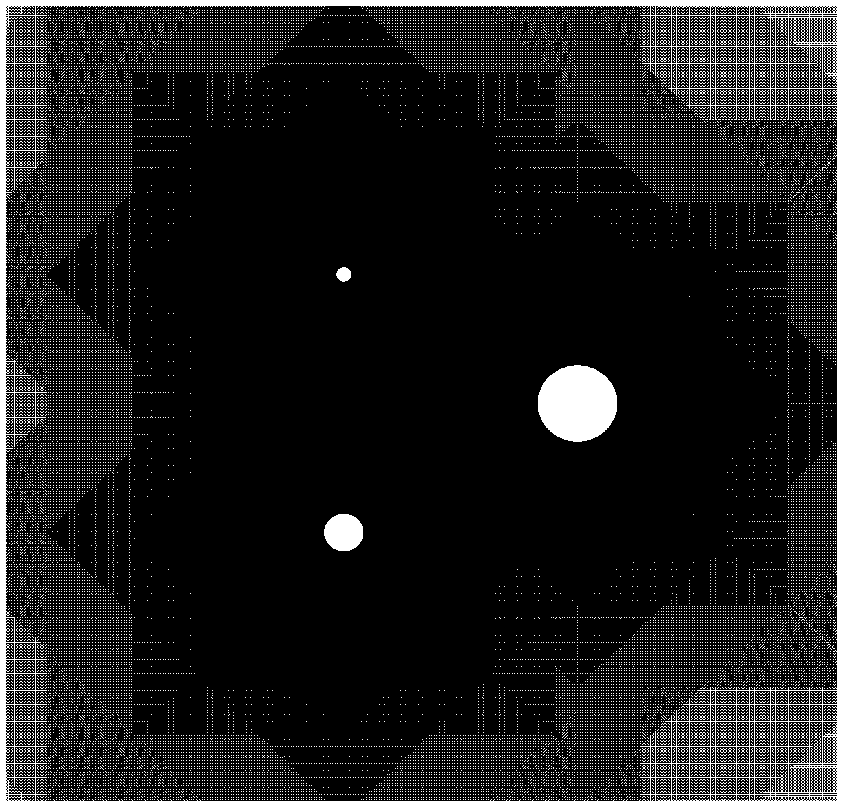
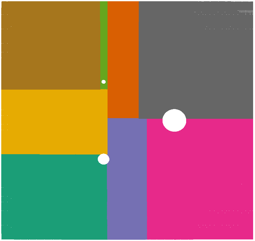
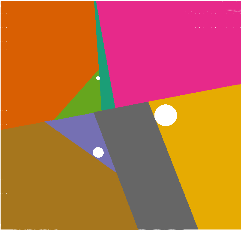
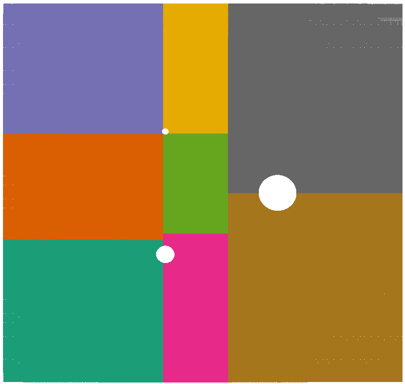
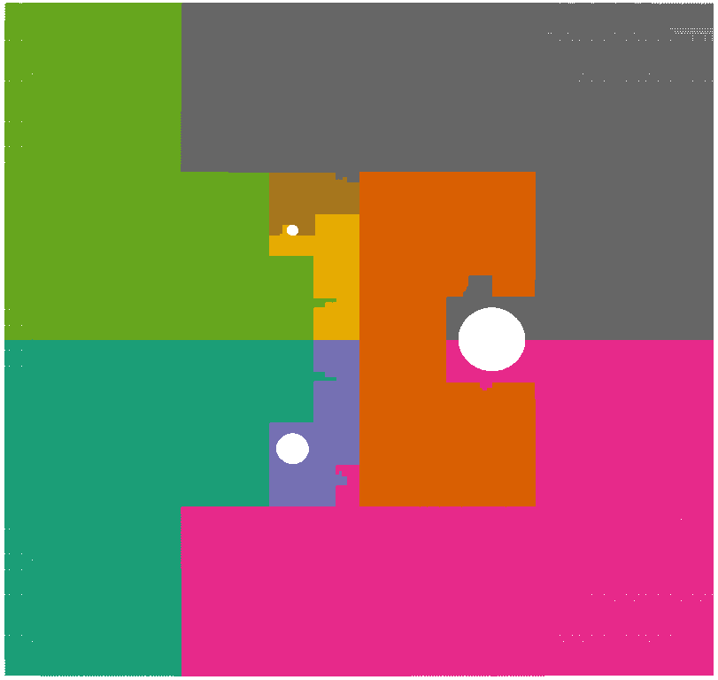
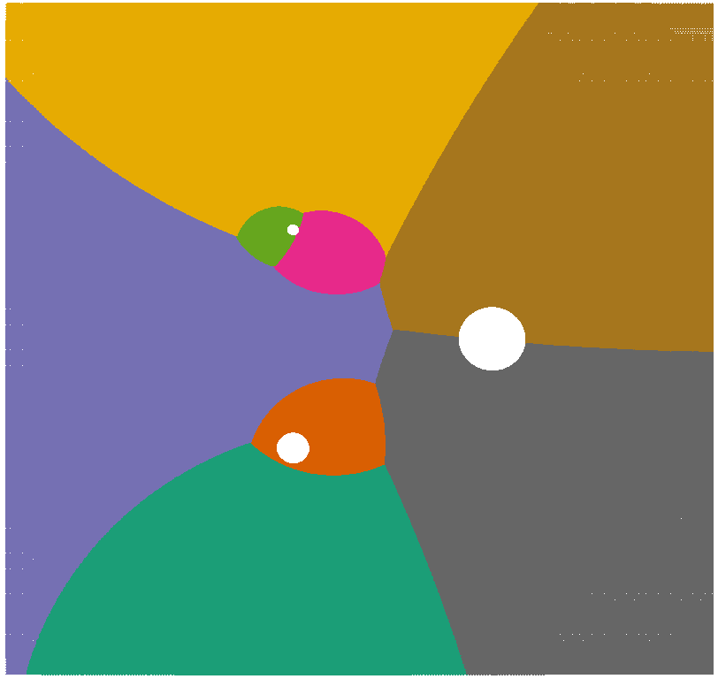
Figure 1: Partition of hugetric-0000 in 8 blocks with different tools. From left to right, the pictures show the input and the results of RCB, RIB, MultiJagged, zoltanSFC and Geographer.

Algorithm 2 shows our main $k$-means algorithm. We first sort and redistribute the points according to a space-filling curve to improve spatial locality (Lines 2 - 2), place initial centers in equal distances on the sorted points (Line 2) and initialize data structures (Lines 2 and 2). Deriving initial centers from the space-filling curve in this way yields a beneficial geometric spread.

The main loop consists of calling Algorithm 1 until the centers converge sufficiently or a maximum number of iterations is reached. New cluster centers are the weighted average of the assigned points; this can be computed efficiently with a local sum and two global MPI vector sum operations (Line 2). Apart from the initial setup, all communication steps are global reduction operations, for which efficient implementations exist. Lines needing communication are marked in blue. Note that the number of blocks the point set is partitioned into is completely independent from the number of parallel processes that are used to do it.

One optimization omitted from the pseudocode for the sake of brevity is random initialization. In the initial phases of $k$-means, cluster centers and influence values change rapidly and the geometric bounds are of little help. However, during these wild fluctuations not as much precision is required as in the later fine-tuning stages. To exploit this effect, each process permutes its local points randomly and then picks the first 100 as initial sample. After each round with center movement, the sample size is doubled. These $\lceil\log_{2}(n_{\text{local}}/100)\rceil$ initialization rounds take about as much time as one round with the full point set, but proceed much further. Starting with only a randomly sampled subset of points does not impact the quality noticeably.

5 Experimental Evaluation

(a) DIMACS graphs (2D)

(b) Climate graphs (2.5D)

(c) Alya and Delaunay (3D)

Figure 2: Aggregated ratios (geometric mean except diameter, see text) of the evaluation metrics for all tools. Baseline: Geographer.

5.1 Implementation

Our graph partitioner Geographer is implemented in C++11 and parallelized with MPI. To increase portability and usability, we develop the partitioner within LAMA [10], a portable framework for distributed linear algebra and other numerical applications. LAMA provides high-level data structures and communication routines for distributed memory, abstracting away the specifics of the MPI communicator and also supporting other parallelization mechanisms. In the course of this work, we contributed several optimized communication routines to LAMA that are used by our partitioner.

5.2 Experimental Settings

5.2.1 Machine

We perform our experiments on Thin Phase 1 nodes of the SuperMUC petascale system at LRZ. Each node is equipped with 32 GB RAM and two Intel Xeon E5-2680 processors (Sandy Bridge) at 2.7 GHz and 8 cores per processor. In our experiments, we allocate one MPI process to each core. Both our code and the evaluated competitors are compiled with GCC 5.4 and parallelized with IBM MPI 1.4. The repository of our implementation will be made public after paper acceptance.

5.2.2 Other Partitioners

We compare Geographer with several established geometric partitioning implementations from the ParMetis (4.0.3) and Zoltan 2 (part of the Trilinos 12.10 Project) toolboxes. The geometric partitioner within the ParMetis package uses space-filling curves, the Zoltan package contains implementations of Recursive Coordinate Bisection (RCB), Recursive Inertial Bisection (RIB), space-filling curves (zoltanSFC) and the MultiJagged algorithm, mentioned in Section 3. Since the ParMetis version of space-filling curves is dominated by the space-filling curves in the Zoltan package, we omit it from the detailed presentation.

5.2.3 Test Data

We evaluate the partitioners on a variety of datasets: a collection of benchmark meshes from the 10th DIMACS implementation challenge [5], 2.5D meshes with node weights from the climate simulations [13] described in Section 1, 3D meshes from the PRACE Unified European Applications Benchmark Suite (UEABS) [37] and Delaunay triangulations of random points in 2 and 3 dimensions.

More precisely, the graphs hugetrace, hugetric and hugebubbles are 2D adaptively refined triangular meshes from the benchmark generator created by Marquardt and Schamberger [28]; they represent synthetic numerical simulations and have approx. 5M to 20M vertices. 333SP, AS365, M6, NACA0015 and NLR are 2D finite element triangular meshes from approx. 3.5M vertices and 11M edges up to approx. 21M vertices and 31M edges. rgg_n are 2D random geometric graph with $2^{n}$ vertices for $n=20,\dots,24$. All these graphs come from the 10th DIMACS Implementation Challenge [5]. The graphs in the DelaunayX series are Delaunay triangulations of X random 2D points in the unit square [23]. The smallest graph in the series has 8M vertices and approximately 24M edges; the largest one has 2B vertices and approximately 6B edges. We also generated five 3D Delaunay triangulations from approx. 1M to 16M vertices using the generator of Funke et al. [19]. The graphs alyaTestCaseA with 9.9 million vertices and alyaTestCaseB with 30.9 million vertices (representing the respiratory system) are from the PRACE benchmark suite [37].

5.2.4 Metrics

We evaluate the generated partitions with respect to the edge cut, the communication volume, the diameter and the SpMV communication time – i. e., the metrics introduced in Section 2. We report both $\max\mathrm{comm}$, the maximum communication volume and $\sum\mathrm{comm}$, the total communication volume.

To evaluate the effect of shape optimization, we also measure the diameter for each block. Since a precise computation of the diameter scales at least quadratically with the number of nodes, we instead use a lower bound generated by executing the first 3 rounds of the iFUB algorithm by Crescenzi et al. [12]. This lower bound is a 2-approximation of the exact diameter, but often already tight.

5.2.5 Other Parameters

In all experiments, we set the number of blocks $k$ to the number of processes $p$ and the maximum imbalance $\epsilon$ to $3\%$, which was respected by all tools. Reported values are averaged over 5 runs to account for random fluctuations.

5.3 Results

For a brief first visual impression of the results of Geographer, RCB, RIB, MultiJagged, and zoltanSFC, see Fig. 1. Recursive coordinate and inertial bisection produce thin, long blocks, MultiJagged produces rectangles with a better aspect ratio, zoltanSFC’s blocks have wrinkled boundaries, balanced k-means produces curved blocks.

5.3.1 Quality

Figure 2 compares the partitions yielded by the tested tools under the metrics edgeCut, maximum and total communication volume and diameter. For easier presentation, we report the relative value compared to Geographer and aggregate the results by graph class using the geometric mean.

In some cases, blocks are disconnected and thus have an infinite diameter. To avoid a potentially infinite mean diameter, we use the harmonic instead of the geometric mean to aggregate the diameter over all blocks.

The first instance class consists of the 2D geometric benchmark meshes from the DIMACS challenge, the second consists of the 2.5D graphs from climate simulations. The third class consists of the alya test case and Delaunay triangulations in the unit cube, all 3D meshes.

In all graph classes, Geographer produces on average the partition with the lowest total communication volume. The advantage is most pronounced on the 2D geometric meshes from the DIMACS collection, but visible also in other classes.

The performance as measured by the edge cut differs: On the DIMACS graphs, Geographer is leading with 15% difference, on the 2.5D and 3D graphs MultiJagged has an advantage of 0.5% and 4%, respectively. Similar developments are visible also for other metrics. Of course, this does not mean that Geographer achieves always the best results, as these are aggregated values.

Strangely, the empirical average communication time within the SpMV benchmarks (timeComm in Figure 2) correlates little with the more established measures. Results fluctuate, but Geographer has on average the smallest SpMV communication time.

Note that the behaviour of balanced $k$-means is stable: If it performs worse on some class, then not by much. None of the evaluated competitors clearly dominates: While MultiJagged, for example, has a lower mean edge (5%) cut on 3D graphs, its performance on the DIMACS graphs is clearly worse, with a 30% higher edge cut.

Detailed results for individual graphs can be found in Tables 1 and 2.

Table 1: Comparison of results for large graphs for $k=p=1024$. Best values are marked in bold.

graph name	tool	time	cut	maxCommVol	$\Sigma$ commVol	diameter	timeSpMVComm
alyaTestCaseB	Geographer	0.358 8	5 823 055	6 508	5 403 716	63	0.000 198 77
n = 30 959 144	HSFC	0.035 270 4	6 613 710	8 275	6 802 889	83	0.000 361 43
	MultiJagged	0.023 448 6	5 364 660	6 062	5 482 086	62	0.000 198 04
	RCB	0.096 641 1	6 188 060	6 526	5 825 470	79	0.000 315 97
delaunay250M	Geographer	0.830 8	2 037 960	2 183	2 033 939	457	3.461${}\cdot{}$10-05
n = 250 000 000	HSFC	0.227 387	2 356 510	2 918	2 349 673	570	0.000 136 38
	MultiJagged	0.228 118	2 118 810	2 214	2 114 657	494	7.432${}\cdot{}$10-05
	RCB	0.857 324	2 118 220	2 211	2 113 916	491	0.000 126 76
delaunay2B	Geographer	6.098 9	5 771 443	6 136	5 754 364	-	-
n = 2 000 000 000	HSFC	1.876 62	6 335 780	6 807	6 314 790	-	-
	MultiJagged	1.716 19	5 994 110	6 164	5 976 573	-	-
	RCB	6.661 74	5 995 910	6 137	5 978 340	-	-
fesom-jigsaw	Geographer	0.774 4	33 135 424	1 539	680 638	392	3.769${}\cdot{}$10-05
n = 14 349 744	HSFC	0.019 375 4	33 749 900	1 500	735 964	339	5.812${}\cdot{}$10-05
	MultiJagged	0.019 648	27 472 100	1 111	641 574	320	4.353${}\cdot{}$10-05
	RCB	0.082 139 5	30 447 900	1 524	642 714	320	6.778${}\cdot{}$10-05
refinedtrace-00006	Geographer	1.506 3	813 450	1 596	1 380 977	1 052	4.095${}\cdot{}$10-05
n = 289 383 634	HSFC	0.516 03	1 044 170	2 856	1 909 341	1 834	0.000 119 55
	MultiJagged	0.260 334	1 063 020	3 790	1 801 389	1 607	7.164${}\cdot{}$10-05
	RCB	1.102 46	930 479	3 864	1 552 315	1 335	0.000 108 35
refinedtrace-00007	Geographer	3.541 7	1 144 423	2 205	1 948 602	1 483	5.198${}\cdot{}$10-05
n = 578 551 252	HSFC	0.812 107	1 467 320	4 054	2 689 631	2 609	0.000 156 08
	MultiJagged	0.570 606	1 521 740	4 644	2 551 801	2 285	8.913${}\cdot{}$10-05
	RCB	2.036 96	1 314 980	6 988	2 189 002	1 898	0.000 146 98

Table 2: Comparison of results for small and medium graphs for $k=p=64$. Best values are marked in bold.

graph name	tool	time	cut	maxCommVol	$\Sigma$ commVol	diameter	timeSpMVComm
333SP	Geographer	1.499 1	32 170	1 203	32 306	205	8.166${}\cdot{}$10-05
n = 3 712 815	HSFC	0.054 583 7	83 162	2 341	83 077	845	6.17${}\cdot{}$10-05
	MultiJagged	0.078 185 9	90 650	3 899	90 793	517	3.396${}\cdot{}$10-05
	RCB	0.081 994 3	59 558	2 291	59 700	357	4.576${}\cdot{}$10-05
AS365	Geographer	0.474 9	51 666	1 114	51 832	274	2.965${}\cdot{}$10-05
n = 3 799 275	HSFC	0.056 799 7	87 274	1 863	87 355	487	6.469${}\cdot{}$10-05
	MultiJagged	0.049 213	64 312	1 796	64 480	364	2.174${}\cdot{}$10-05
	RCB	0.101 785	55 880	1 075	56 040	313	5.214${}\cdot{}$10-05
M6	Geographer	0.292 1	51 971	1 145	52 131	259	2.771${}\cdot{}$10-05
n = 3 501 776	HSFC	0.044 984 5	82 905	1 749	82 938	416	6.417${}\cdot{}$10-05
	MultiJagged	0.041 304	58 270	1 080	58 430	310	2.289${}\cdot{}$10-05
	RCB	0.085 696 8	56 867	1 052	57 027	301	5.229${}\cdot{}$10-05
NACA0015	Geographer	0.106 6	27 841	549	27 997	152	2.426${}\cdot{}$10-05
n = 1 039 183	HSFC	0.012 555 2	56 902	1 367	56 897	370	5.145${}\cdot{}$10-05
	MultiJagged	0.014 093 9	40 314	759	40 476	244	1.941${}\cdot{}$10-05
	RCB	0.031 087	29 484	603	29 638	162	3.16${}\cdot{}$10-05
NLR	Geographer	0.374 4	56 805	1 073	56 969	281	2.893${}\cdot{}$10-05
n = 4 163 763	HSFC	0.054 883 9	85 740	1 704	85 803	377	6.383${}\cdot{}$10-05
	MultiJagged	0.059 456 9	61 034	1 102	61 193	306	2.368${}\cdot{}$10-05
	RCB	0.113 787	60 703	1 170	60 863	306	4.799${}\cdot{}$10-05
alyaTestCaseA	Geographer	0.966	894 845	18 341	841 593	113	0.000 214 97
n = 9 938 375	HSFC	0.122 195	988 168	21 325	1 001 416	132	0.000 356 05
	MultiJagged	0.080 141 5	839 540	17 798	839 437	107	0.000 250 6
	RCB	0.172 015	847 188	17 726	839 377	108	0.000 274 82
alyaTestCaseB	Geographer	1.865 7	1 869 558	38 203	1 774 168	163	0.000 329 37
n = 30 959 144	HSFC	0.395 728	1 857 670	39 351	1 880 792	171	0.000 589 69
	MultiJagged	0.255 547	1 772 580	37 435	1 785 528	156	0.000 511 83
	RCB	0.577 578	1 784 790	37 447	1 785 598	167	0.000 574 01
delaunay017M	Geographer	0.733 2	122 875	2 235	122 634	476	3.013${}\cdot{}$10-05
n = 17 000 000	HSFC	0.249 101	131 407	2 428	131 012	549	0.000 103 83
	MultiJagged	0.178 99	125 088	2 302	124 823	489	3.832${}\cdot{}$10-05
	RCB	0.385 619	124 789	2 263	124 545	499	0.000 106 32
fesom-f2glo04	Geographer	0.448 2	4 758 930	1 590	66 472	547	2.948${}\cdot{}$10-05
n = 5 945 730	HSFC	0.068 410 1	7 677 820	2 372	108 910	957	4.574${}\cdot{}$10-05
	MultiJagged	0.079 680 6	5 866 330	2 263	85 789	740	3.185${}\cdot{}$10-05
	RCB	0.137 691	5 596 840	1 755	79 220	631	4.222${}\cdot{}$10-05
fesom-fron	Geographer	0.509 8	3 870 505	1 565	61 576	731	3.32${}\cdot{}$10-05
n = 5 007 727	HSFC	0.054 661 7	5 272 540	1 993	90 305	1 067	3.205${}\cdot{}$10-05
	MultiJagged	0.060 941 6	4 214 460	1 485	70 794	788	2.691${}\cdot{}$10-05
	RCB	0.090 324 9	4 365 920	1 846	74 330	706	3.441${}\cdot{}$10-05
fesom-jigsaw	Geographer	1.085 4	8 444 620	4 225	166 006	6 306	4.233${}\cdot{}$10-05
n = 14 349 744	HSFC	0.183 937	8 224 760	4 269	177 071	2 159	0.000 121 37
	MultiJagged	0.176 129	6 185 490	3 078	142 214	1 843	4.101${}\cdot{}$10-05
	RCB	0.393 419	8 637 620	3 980	173 583	2 800	0.000 123 33
hugebubbles-00020	Geographer	2.584 8	47 763	1 636	81 556	1 048	3.1${}\cdot{}$10-05
n = 21 198 119	HSFC	0.281 46	63 053	2 561	118 785	2 002	7.507${}\cdot{}$10-05
	MultiJagged	0.283 137	60 958	2 430	105 714	1 453	3.191${}\cdot{}$10-05
	RCB	0.612 614	57 482	2 003	98 404	1 299	7.898${}\cdot{}$10-05
hugetrace-00020	Geographer	1.483 3	43 522	1 471	74 122	948	3.102${}\cdot{}$10-05
n = 16 002 413	HSFC	0.203 32	50 800	2 081	98 367	1 585	5.583${}\cdot{}$10-05
	MultiJagged	0.192 364	50 493	1 872	86 699	1 117	2.76${}\cdot{}$10-05
	RCB	0.393 817	50 851	1 911	84 526	1 084	3.904${}\cdot{}$10-05
hugetric-00020	Geographer	0.820 6	29 298	972	49 899	615	2.878${}\cdot{}$10-05
n = 7 122 792	HSFC	0.157 777	39 373	1 658	72 388	1 210	5.725${}\cdot{}$10-05
	MultiJagged	0.092 852 5	39 382	2 203	67 949	899	3.033${}\cdot{}$10-05
	RCB	0.176 951	35 512	1 364	60 706	810	5.482${}\cdot{}$10-05
rdg-3d	Geographer	0.324 3	1 481 602	12 683	761 610	45	0.000 251 51
n = 4 194 304	HSFC	0.046 123 2	1 596 600	13 391	821 701	50	0.000 328 72
	MultiJagged	0.057 363 3	1 537 820	12 552	790 899	48	0.000 278 77
	RCB	0.088 234 2	1 537 980	12 558	791 086	48	0.000 297 71

5.3.2 Scaling and Running Time

(a) Weak scaling for DelaunayX graph series.

(b) Strong scaling for Delaunay2B graph

Figure 3: Scaling results on DelaunayX regarding (a) strong and (b) weak scaling.

Weak Scaling

Fig. 3(a) shows a direct comparison of weak scaling performance on the DelauanyX graph series. We start with 32 processes ($p$) and blocks ($k$) on 8 million vertices and repeatedly double both until we reach 8 192 processes on 2 billion vertices, keeping the ratio fixed at approx 250 000 vertices per process. Geographer exhibits similar behavior as MultiJagged and zoltanSFC: they scale almost perfectly up to 1024 PEs, then increase roughly by a factor of two over the next three doublings. The recursive methods RIB and RCB show an immediate increase in running time with larger inputs and scale especially poorly on more than 1 024 processes, more than doubling the running time for each doubling of input and process count. A comparison of running times on all graphs can be seen in Fig. 4. The scaling behavior of the different tools follows similar trends as on the DelaunayX series. Fitted trend lines show a better weak scaling behavior of Geographer than on Delaunay graphs alone, which may also be an artifact of the higher number of smaller graphs in our collection.

Strong Scaling

We perform strong scaling experiments (see Fig. 3(b)) with the largest graph at our disposal, Delaunay2B. With 2 billion vertices, it is small enough to fit into the memory of 1 024 processing elements but also sufficiently large to partition it into 16 384 blocks. Note that our experiments are not, strictly speaking, strong scaling, as we increase the number of blocks along with the number of processors.

Similarly to the weak scaling results, Geographer, MultiJagged and zoltanSFC have similar scaling behavior: almost perfect scalability for up to 4 096 PEs (MultiJagged also for 8 192). RCB and RIB start with the slowest running times, around $6.5$ seconds for $k=1024$ and climb to $23$ seconds for $k=16384$ showing poor scalability. For all tools, the running time increases from 8 192 to 16 384 processes; we attribute this to the SuperMUC architecture: an island in SuperMUC contains 8 192 cores and communication is more expensive across islands.

Components

The main parts of Geographer contributing to the running time are the initial partition with a Hilbert curve, the redistribution of coordinates according to this initial partition and finally the balanced $k$-means itself. As the number of processes increases, the relative share of these components changes: For small instances, the computation of Hilbert indices and the balanced $k$-means iterations constitute a majority of the time, while for higher number of processes, the redistribution step dominates. For example, when partitioning Delaunay2B with 1024 processes, data redistribution and $k$-means take $32\%$ respective $47\%$ of the time. For the same graph and 16384 processes, redistribution takes $46\%$ and $k$-means $42\%$ of the total running time.

6 Conclusions

Figure 4: Comparison of running times. Each dot represents the running time of one tool on one graph. For comparable results, we aimed for 250 000 points per block, selecting the number of blocks $k$ (and processes $k)$ separately for each graph. Since some tools only support powers of two for the number of blocks, we select the power of two which results in the number of local points closest to our target of 250 000.

We designed and implemented a balanced, scalable version of $k$-means for partitioning geometric meshes. Combined with space-filling curves for initialization, it scales to thousands of processors and billions of vertices, partitioning them in a matter of seconds.

An evaluation on a wide range of input meshes shows that the total communication volume and resulting SpMV communication time of the resulting partitions is on average 5-15% better than those of state-of-the-art competitors. This difference is most pronounced on meshes from the DIMACS benchmark collection, but also measurable on graphs from climate simulations and 3D meshes. Concerning the edge cut, another common metric to evaluate graph partitioners, MultiJagged also performs well, giving the best results on 3D meshes. No partitioner dominates on all point sets.

Future work will be concerned with further improving quality and scalability, in particular for 3D meshes. A faster redistribution routine, necessary to achieve scalability for a higher number of processes, is also of independent interest. Finding high-quality embeddings of non-geometric graphs into some geometric space in a scalable manner is promising, too. This preprocessing would allow to apply Geographer to non-geometric graphs as well.

References

- [1] David Arthur and Sergei Vassilvitskii. k-means++: The advantages of careful seeding. In Proceedings of the eighteenth annual ACM-SIAM symposium on Discrete algorithms, pages 1027–1035. Society for Industrial and Applied Mathematics, 2007.
- [2] Franz Aurenhammer and Herbert Edelsbrunner. An optimal algorithm for constructing the weighted voronoi diagram in the plane. Pattern Recognition, 17(2):251–257, 1984.
- [3] M. Axtmann, A. Wiebigke, and P. Sanders. Lightweight MPI Communicators with Applications to Perfectly Balanced Schizophrenic Quicksort. In Proc. 32nd International Parallel and Distributed Processing Symp. (IPDPS 2018), 2018. To appear.
- [4] Olivier Bachem, Mario Lucic, Hamed Hassani, and Andreas Krause. Fast and provably good seedings for k-means. In Advances in Neural Information Processing Systems, pages 55–63, 2016.
- [5] David Bader, Henning Meyerhenke, Peter Sanders, and Dorothea Wagner, editors. Proc. of the 10th DIMACS Implementation Challenge, Contemporary Mathematics. American Mathematical Society, 2012.
- [6] Michael Bader. Space-Filling Curves: An Introduction with Applications in Scientific Computing. Springer Publishing Company, Inc., 2012.
- [7] M. J. Berger and S. H. Bokhari. A partitioning strategy for nonuniform problems on multiprocessors. IEEE Trans. Comput., 36(5):570–580, May 1987.
- [8] C.E. Bichot and P. Siarry. Graph Partitioning. ISTE. Wiley, 2013.
- [9] E. G. Boman, U. V. Catalyurek, C. Chevalier, and K. D. Devine. The Zoltan and Isorropia parallel toolkits for combinatorial scientific computing: Partitioning, ordering, and coloring. Scientific Programming, 20(2):129–150, 2012.
- [10] Thomas Brandes, Eric Schricker, and Thomas Soddemann. The LAMA Approach for Writing Portable Applications on Heterogeneous Architectures. Springer Berlin Heidelberg, 2017.
- [11] Aydin Buluç, Henning Meyerhenke, Ilya Safro, Peter Sanders, and Christian Schulz. Recent advances in graph partitioning. In Lasse Kliemann and Peter Sanders, editors, Algorithm Engineering - Selected Results and Surveys, volume 9220 of Lecture Notes in Computer Science, pages 117–158. 2016.
- [12] Pilu Crescenzi, Roberto Grossi, Michel Habib, Leonardo Lanzi, and Andrea Marino. On computing the diameter of real-world undirected graphs. Theoretical Computer Science, 514:84–95, 2013.
- [13] S. Danilov, D. Sidorenko, Q. Wang, and T. Jung. The finite-volume sea ice–ocean model (fesom2). Geoscientific Model Development, 10(2):765–789, 2017.
- [14] Mehmet Deveci, Sivasankaran Rajamanickam, Karen D. Devine, and Ümit V. Çatalyürek . Multi-jagged: A scalable parallel spatial partitioning algorithm. IEEE Trans. Parallel Distrib. Syst., 27:803–817, 2016.
- [15] R. Diekmann, R. Preis, F. Schlimbach, and C. Walshaw. Shape-optimized mesh partitioning and load balancing for parallel adaptive FEM. Parallel Computing, 26:1555–1581, 2000.
- [16] Jonathan Drake and Greg Hamerly. Accelerated k-means with adaptive distance bounds. In 5th NIPS workshop on optimization for machine learning, pages 42–53, 2012.
- [17] Charles Elkan. Using the triangle inequality to accelerate k-means. In Proceedings of the 20th International Conference on Machine Learning (ICML-03), pages 147–153, 2003.
- [18] Lin Fu, Sergej Litvinov, Xiangyu Y. Hu, and Nikolaus A. Adams. A novel partitioning method for block-structured adaptive meshes. J. Comput. Physics, 341:447–473, 2017.
- [19] Daniel Funke, Sebastian Lamm, Peter Sanders, Christian Schulz, Darren Strash, and Moritz von Looz. Communication-free massively distributed graph generation. In Proc. 32nd International Parallel and Distributed Processing Symp. (IPDPS 2018), 2018. To appear.
- [20] Greg Hamerly. Making k-means even faster. In Proceedings of the 2010 SIAM international conference on data mining, pages 130–140. SIAM, 2010.
- [21] Bruce Hendrickson and Tamara G. Kolda. Graph partitioning models for parallel computing. Parallel Comput., 26(12):1519–1534, 2000.
- [22] Bruce Hendrickson and Robert Leland. An improved spectral graph partitioning algorithm for mapping parallel computations. SIAM Journal on Scientific Computing, 16(2):452–469, 1995.
- [23] Manuel Holtgrewe, Peter Sanders, and Christian Schulz. Engineering a scalable high quality graph partitioner. In 24th Int. Parallel and Distributed Processing Symp. (IPDPS), 2010.
- [24] Jan Hungershöfer and Jens-Michael Wierum. On the quality of partitions based on space-filling curves. In Proceedings of the International Conference on Computational Science-Part III, ICCS ’02, pages 36–45, London, UK, UK, 2002. Springer-Verlag.
- [25] Shad Kirmani and Padma Raghavan. Scalable parallel graph partitioning. In William Gropp and Satoshi Matsuoka, editors, International Conference for High Performance Computing, Networking, Storage and Analysis, SC’13, Denver, CO, USA - November 17 - 21, 2013, pages 51:1–51:10. ACM, 2013.
- [26] Stuart P. Lloyd. Least squares quantization in PCM. IEEE Transactions on Information Theory, 28(2):129–136, 1982.
- [27] Bruno R. C. Magalhães, Farhan Tauheed, Thomas Heinis, Anastasia Ailamaki, and Felix Schürmann. An Efficient Parallel Load-Balancing Framework for Orthogonal Decomposition of Geometrical Data, pages 81–97. Springer International Publishing, Cham, 2016.
- [28] O. Marquardt and S. Schamberger. Open benchmarks for load balancing heuristics in parallel adaptive finite element computations. In Proc. of the International Conference on Parallel and Distributed Processing Techniques and Applications, (PDPTA’05), pages 685–691. CSREA Press, 2005.
- [29] Henning Meyerhenke. Shape optimizing load balancing for mpi-parallel adaptive numerical simulations. In David A. Bader, Henning Meyerhenke, Peter Sanders, and Dorothea Wagner, editors, Proc. of the 10th DIMACS Implementation Challenge – Graph Partitioning and Graph Clustering, Contemporary Mathematics. American Mathematical Society, 2013.
- [30] Henning Meyerhenke, Burkhard Monien, and Thomas Sauerwald. A new diffusion-based multilevel algorithm for computing graph partitions. Journal of Parallel and Distributed Computing, 69(9):750–761, 2009. Best Paper Awards and Panel Summary: IPDPS 2008.
- [31] Henning Meyerhenke, Burkhard Monien, and Stefan Schamberger. Graph partitioning and disturbed diffusion. Parallel Computing, 35(10–11):544–569, 2009.
- [32] Henning Meyerhenke, Peter Sanders, and Christian Schulz. Parallel graph partitioning for complex networks. IEEE Trans. Parallel Distrib. Syst., 28(9):2625–2638, 2017.
- [33] Henning Meyerhenke and Thomas Sauerwald. Beyond good partition shapes: An analysis of diffusive graph partitioning. Algorithmica, 64(3):329–361, 2012.
- [34] Henning Meyerhenke and Stefan Schamberger. A parallel shape optimizing load balancer. In Proc. of the 12th International Euro-Par Conference, volume 4128 of LNCS, pages 232–242. Springer-Verlag, 2006.
- [35] K. W. Morton and D. F. Mayers. Numerical Solution of Partial Differential Equations: An Introduction. Cambridge University Press, New York, NY, USA, 2005.
- [36] François Pellegrini. Scotch and PT-scotch graph partitioning software: An overview. In Uwe Naumann and Olaf Schenk, editors, Combinatorial Scientific Computing, pages 373–406. CRC Press, 2012.
- [37] PRACE. Unified european applications benchmark suite. http://www.prace-ri.eu/ueabs?lang=en. Accessed: 2010-09-30.
- [38] V. Sarkar, W. Harrod, and A. E Snavely. Software challenges in extreme scale systems. Journal of Physics: Conference Series, 180(1):012045, 2009.
- [39] K. Schloegel, G. Karypis, and V. Kumar. Graph partitioning for high performance scientific simulations. In The Sourcebook of Parallel Computing, pages 491–541. Morgan Kaufmann, 2003.
- [40] Kirk Schloegel, George Karypis, and Vipin Kumar. Parallel static and dynamic multi-constraint graph partitioning. Concurrency and Computation: Practice and Experience, 14(3):219–240, 2002.
- [41] David Sculley. Web-scale k-means clustering. In Proceedings of the 19th international conference on World wide web, pages 1177–1178. ACM, 2010.
- [42] H.D. Simon. Partitioning of unstructured problems for parallel processing. Computing Systems in Engineering, 2(2):135 – 148, 1991. Parallel Methods on Large-scale Structural Analysis and Physics Applications.
- [43] G. M. Slota, S. Rajamanickam, Karen Devine, and K. Madduri. Partitioning trillion-edge graphs in minutes. In Proc. 31st International Parallel and Distributed Processing Symp. (IPDPS 2017), 2017.
- [44] Valerie E. Taylor and Bahram Nour‐Omid. A study of the factorization fill‐in for a parallel implementation of the finite element method. International Journal for Numerical Methods in Engineering, 37(22):3809–3823.
- [45] C. Walshaw and M. Cross. Jostle: Parallel multilevel graph-partitioning software – an overview. In F. Magoules, editor, Mesh Partitioning Techniques and Domain Decomposition Techniques, pages 27–58. Civil-Comp Ltd., 2007. (Invited chapter).
- [46] Roy D. Williams. Performance of dynamic load balancing algorithms for unstructured mesh calculations. Concurrency: Practice and Experience, 3(5):457–481, 1991.