Single-Channel Blind Source Separation for Singing Voice Detection: A Comparative Study

Abstract

We propose a novel unsupervised singing voice detection method which use single-channel Blind Audio Source Separation (BASS) algorithm as a preliminary step. To reach this goal, we investigate three promising BASS approaches which operate through a morphological filtering of the analyzed mixture spectrogram. The contributions of this paper are manyfold. First, the investigated BASS methods are reworded with the same formalism and we investigate their respective hyperparameters by numerical simulations. Second, we propose an extension of the KAM method for which we propose a novel training algorithm used to compute a source-specific kernel from a given isolated source signal. Second, the BASS methods are compared together in terms of source separation accuracy and in terms of singing voice detection accuracy when they are used in our new singing voice detection framework. Finally, we do an exhaustive singing voice detection evaluation for which we compare both supervised and unsupervised singing voice detection methods. Our comparison explores different combination of the proposed BASS methods with new features such as the new proposed KAM features and the scattering transform through a machine learning framework and also considers convolutional neural networks methods.

1 Introduction

Audio source separation aims at recovering the isolated signals of each source (i.e. each instrumental part) which composes an observed mixture [1, 2]. Although humans can easily recognize the different sound entities which are active at each time instant, this task remains challenging when it has to be automatically completed by an unsupervised algorithm. Mathematically speaking, Blind Audio Source Separation (BASS) is an “ill-posed problem” in the sense of Hadamard [3], however it remains intensively studied since many decades [1, 4, 5, 6, 7]. In fact, BASS is full of interest because it can find many applications such as music remixing (karaoke, re-spatialization, source manipulation), and signal enhancement (denoising). Thus, BASS can directly be used as a part of a signal detection method (i.e. singing voice), in relation with the source separation model. This study, addresses the single-channel blind case, when several sources $s_{i}$ ($i\in[1,I]$, with $I\geq 2$) are present in a unique instantaneous mixture $x$ expressed as:

$$x(t)=\displaystyle\sum_{i=1}^{I}s_{i}(t).$$ (1)

Despite the simplicity of the mixture model of Eq. (1), this configuration is more challenging to solve than multi-channel mixtures. In fact, multi-channel methods such as [8, 2] require at least 2 distinct observed mixtures with a sufficient orthogonality in the time-frequency plane between the sources, to provide satisfying separation results. As we address the underdetermined case (where the number of sources is greater than the number of observations), Independent Component Analysis (ICA) methods can neither be directly used [1]. Moreover, methods inspired by Computational Auditory Scene Analysis (CASA) [9], such as [10, 5, 11], are often not robust enough for processing real-world music mixtures and should be addressed through an Informed Source Separation (ISS) framework using side-information in a coder-decoder scheme as proposed in [12].

For all these reasons, we focus on another class of robust BASS methods based on time-frequency representation morphological filtering. These methods assume that the foreground voice and the instrumental music background have significantly different time-frequency regularities which can be exploited to assign each time-frequency point to a source. To illustrate this idea, vertical lines can be observed in a drum set spectrogram due the spectral regularities at each instant, contrarily to an harmonic source which has horizontal lines due to the regularities over time of each active frequency (i.e. the partials). A recent comparative study [13] leads us to three very promising approaches which can be summarized as follows.

1) Total variation approach proposed by Jeong and Lee [14], aims at minimizing a convex auxiliary function, related to the temporal continuity (for harmonic sources), the spectral continuity (for percussive sounds) and the sparsity for the leading singing voice. The solutions provides estimates of the spectrogram of each source.

2) Robust Principal Component Analysis (RPCA)[15] is used for voice/music separation in [16]. This technique decomposes the mixture spectrogram into two matrices: a low rank matrix associated to the spectrogram of the repetitive musical background (the accompaniment), and a sparse matrix associated to the lead instrument which plays the melody.

3) Kernel Additive Modeling (KAM) as formalized in [17], unifies several BASS approaches into the same framework: REPET [18] and Harmonic Percussive Source Separation (HPSS) through median filtering [19]. Both methods use the source-specific regularities in their time-frequency representations to compute a source separation mask. Hence, each source is characterized by a kernel which models the vicinity of each time-frequency point in a spectrogram. This allows to estimate each source using a median filter based on its specific kernel. This idea was extended through other source-specific kernels in [17, 20, 21, 22] and in the present paper.

Thus, the purpose of this work is first to unify these BASS methods into the same framework to segregate a monaural mixture into 3 components corresponding to the percussive part, the harmonic background and the singing voice. Second, we introduce a new unsupervised singing voice detection method which can use any BASS method as a preprocessing step. Finally, the BASS methods are compared together in terms of separation quality and in terms of singing voice detection accuracy. Our evaluation also considers a comparison with supervised state-of-the-art singing voice detection methods such as [23] which uses deep Convolutional Neural Networks (CNN).

This paper is organized as follows. In Section 2, we shortly describe the proposed BASS methods with an extension of the KAM method for source-specific kernel training. In Section 3, we introduce our framework for singing voice detection based on BASS. In Section 4, comparative results for source separation and singing voice detection are presented. Finally, conclusion and future works are discussed in Section 5.

2 Source separation through spectrogram morphological filtering

2.1 Typical Algorithm and Oracle Method

We investigate three promising BASS methods based on morphological filtering of the mixture’s spectrogram (defined as the squared modulus of its Short-Time Fourier Transform (STFT) [24]). Each method aims at estimating the real-valued non-negative matrices of size $F\times T$, which correspond to the source separation masks $M_{v}$, $M_{h}$ and $M_{p}$, respectively associated to the voice, the harmonic accompaniment and the percussive part. Thus, a typical algorithm using any BASS method, can be formulated by Algorithm 1.

Data: $x$: observed mixture, $\alpha$: user parameter (cf. Fig. 1)

Result: $\hat{s}_{i}$: estimated source signals, $\hat{S}_{i}$: STFTs of the estimated sources

$X\leftarrow\text{STFT}(x)$

$(M_{v},M_{h},M_{p})\leftarrow\text{BASSMethod}\left(|X|^{2}\right)$

for $i\in\{v,h,p\}$ do

       $\hat{S}_{i}\leftarrow\frac{|M_{i}|^{\alpha}}{\sum_{j\in\{v,h,p\}}|M_{j}|^{\alpha}}$ X

       $\hat{s}_{i}\leftarrow\text{invSTFT}(\hat{S}_{i})$

      

Algorithm 1 Typical BASS algorithm based on morphological filtering. $\text{STFT}()$ and $\text{invSTFT}()$ compute respectively the STFT and its inverse from a discrete-time signal.

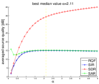
(a) objective results

(b) objective results

(c) perceptual results

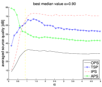
(d) perceptual results

Figure 1: Effect of parameter $\alpha$ in Algorithm 1 on the source separation quality of a musical mixture made of 3 sources. Measures are expressed in terms of BSS Eval v2 [25] (a), BSS Eval v3 [26] (b)-(d) which also assess the perceptual quality (high values are better).

In this algorithm, $\frac{|M_{i}|^{\alpha}}{\sum_{j\in\{v,h,p\}}|M_{j}|^{\alpha}}$ approximates the parameterized Wiener filter [27] of the source $i$, for which an optimal value of $|M_{i}|^{\alpha}$ in the minimal Mean Squared Error (MSE) sense, corresponds to the source’s spectral density [28]. In practice, the effect of parameter $\alpha$ on the separation quality is illustrated in Fig. 1 which shows the results provided by Algorithm 1 when applied on a mixture made of 3 audio sources (voice, keyboard/synthesizer and drums). This experiment uses an oracle BASS method (i.e. original sources are assumed known) which sets the source mask as the modulus of the STFT of each source such as $M_{i}=|S_{i}|$. The highest median of the MSE-based results (cf. Fig. 1 (a)-(b)) is reached with $\alpha\approx 2$. Interestingly, best perceptual results are reached with $\alpha\approx 1$ (cf. Fig. 1 (c)-(d)). A detailed description of Signal-to-Interference Ratio (SIR), Signal-to-Artifact Ratio (SAR) and Signal-to-Distortion Ratio (SDR) measures can be found in [25, 26]. The Reconstruction Quality Factor (RQF) (cf. Fig. 1 (a)) is defined as[29]: $\text{RQF}(s,\hat{s})=10\log_{10}\left(\frac{\sum_{n}|s[n]|^{2}}{\sum_{n}|s[n]-\hat{s}[n]|^{2}}\right)$, where $s$ and $\hat{s}$ stand respectively for the original source and its estimation.

2.2 Total Variation Approach

Blind source separation can be addressed as an optimization problem solved using a total variation regularization. This approach has successfully been used in image processing for noise removal [30]. It consists in minimizing a convex auxiliary function which depends on regularization parameters $\lambda_{1}$, $\lambda_{2}$ to control the relative importance of the smoothness of the expected masks $M_{h}$ and $M_{p}$ respectively over time and frequencies. This choice is justified by the harmonic or spectral stability of $M_{h}$ and $M_{p}$, and the sparsity of $M_{v}$. Being a discrete-time signal $x[n]$ and its discrete STFT, $X[n,m]$, where $n=1...T$ and $m=1...F$, are the time and frequency indices such as $t=nT_{s}$ and $\omega=2\pi\frac{m}{FT_{s}}$, $T_{s}$ being the sampling period. The Jeong-Lee-14 method [14] minimizes the following auxiliary function:

$$J(M_{v},M_{h},M_{p}) =\frac{1}{2}\sum_{n,m}(M_{h}[n-1,m]-M_{h}[n,m])^{2}$$

$$+\frac{\lambda_{1}}{2}\sum_{n,m}(M_{p}[n,m-1]-M_{p}[n,m])^{2}$$

$$+\lambda_{2}\sum_{n,m}\left|M_{v}[n,m]\right|$$ (2)

subject to: $$M_{v}+M_{h}+M_{p}=|X|^{2\gamma}$$

with: $$M_{v}[n,m],M_{h}[n,m],M_{p}[n,m]\geq 0.$$

Hence, solving $\frac{\partial J(M_{v},M_{h},M_{p})}{\partial M_{h}}=0$ and $\frac{\partial J(M_{v},M_{h},M_{p})}{\partial M_{p}}=0$, allows to derive update rules which lead to an iterative method formulated by Algorithm 2 [14]. According to the authors, the best separation results are obtained with 16 kHz-sampled signal mixtures, using 64 ms-long $\frac{3}{4}$-overlapped analysis frames, in combination with a 120 Hz high-pass filter applied on the mixture, and using method parameters: $\lambda_{1}=0.25$, $\lambda_{2}=10^{-1}\lambda_{1}$, $\gamma=\frac{1}{4}$ (i.e. $\alpha=2$) and $N_{\text{iter}}=200$.

Data: $x$: observed mixture, $\lambda_{1},\lambda_{2},\gamma$: user parameters, $N_{\text{iter}}$: number of iterations

Result: $\hat{s}_{i}$: estimated source signals, $\hat{S}_{i}$: STFTs of the estimated sources

$X\leftarrow\text{STFT}(x)$

$W\leftarrow|X|^{2\gamma}$

$M_{h}\leftarrow 0$, $M_{p}\leftarrow 0$

for $it\leftarrow 1$ to $N_{\text{iter}}$ do

       $M_{h}{\scriptstyle[n,m]}\leftarrow\min\!\left(\!\frac{M_{h}{\scriptstyle[n+1,m]}+M_{h}{\scriptstyle[n-1,m]}}{2}+\frac{\lambda_{1}}{2},\right.$

       $\left.W{\scriptstyle[n,m]}-M_{p}{\scriptstyle[n,m]}\right)$

       $M_{p}{\scriptstyle[n,m]}\leftarrow\min\!\left(\!\frac{M_{p}{\scriptstyle[n,m+1]}+M_{p}{\scriptstyle[n,m-1]}}{2}+\frac{\lambda_{1}}{2\lambda_{2}},\right.$

       $\left.W{\scriptstyle[n,m]}-M_{h}{\scriptstyle[n,m]}\right)$

      

$M_{v}\leftarrow W-(M_{h}+M_{p})$

for $i\in\{v,h,p\}$ do

       $\hat{S}_{i}\leftarrow\frac{|M_{i}|^{\frac{1}{2\gamma}}}{\sum_{i}|M_{i}|^{\frac{1}{2\gamma}}}$ X

       $\hat{s}_{i}\leftarrow\text{invSTFT}(\hat{S}_{i})$

      

Algorithm 2 Jeong-Lee-14’s BASS algorithm.

2.3 Robust Principal Component Analysis

In a musical mixture, the background accompaniment is often repetitive while the main melody played by the singing voice contains harmonic and frequency modulated components with a non-redundant structure. This property allows a decomposition of the mixture spectrogram $W=|X|^{2}$ into two distinct matrices where the background accompaniment spectrogram is associated to a low rank matrix, and the foreground singing voice is associated to a sparse matrix (i.e. where most of the elements are zeros or close to zero). Thus, a solution inspired from the image processing methods is provided by RPCA [15] which decomposes a non-negative matrix $W$ into a sum of two matrices $M_{hp}$ and $M_{v}$, through an optimization process. It can be formulated as the minimization of the following auxiliary function expressed as:

$$J(M_{hp},M_{v}) =||M_{hp}||_{*}+\lambda||M_{v}||_{1}$$ (3)

subject to: $$W=M_{hp}+M_{v}$$

with $||M_{hp}||_{*}=\sum_{k}\sigma_{k}(M_{hp})$ the nuclear norm of matrix $M_{hp}$, $\sigma_{k}$ being its $k$-th singular value, and $||M_{v}||_{1}=\sum_{n,m}|M_{v}[n,m]|$ being the $l_{1}$-norm of the matrix $M_{v}$. Here, $\lambda$ denotes a damping parameter which should be optimally chosen as $\lambda=\frac{1}{\sqrt{\max(T,F)}}$ [15, 16]. Eq. (3) is then solved by the augmented Lagrangian method which leads to the following new auxiliary function (adding new variable $Y$):

$$J(M_{hp},M_{v},Y)=||M_{hp}||_{*}+\lambda||M_{v}||_{1}+\\ \langle Y,W-M_{hp}-M_{v}\rangle+\frac{\mu}{2}||W-M_{hp}-M_{v}||^{2}_{F}$$ (4)

where $\langle a,b\rangle=a^{T}b$, and $\mu$ is a Lagrangian multiplier. Thus, Eq. (4) is efficiently minimized through the Principal Component Pursuit algorithm [31] formulated by Algorithm 3. Our empirical experiments on real-word audio signals show that $\mu=10\lambda$ and $N_{\text{iter}}=1000$ provide satisfying results.

Data: $W$: spectrogram of the mixture, $\lambda,\mu$: damping parameters, $N_{\text{iter}}$: number of iterations

Result: $L=M_{hp}$, $S=M_{v}$: separation masks for the voice (v) and the music accompaniment (hp)

$S\leftarrow 0$, $Y\leftarrow 0$

for $it\leftarrow 1$ to $N_{\text{iter}}$ do

       $L\leftarrow\text{argmin}_{L}J(L,S,Y)$

       $S\leftarrow\text{argmin}_{S}J(L,S,Y)$

       $Y\leftarrow Y+\mu(W-L-S)$

Algorithm 3 Principal Component Pursuit by alternating directions algorithm [31].

For the sake of computation efficiency, it can be shown that the update rules in Algorithm 3 can be computed as [15]:

$$\text{argmin}_{L}J(L,S,Y) =\mathcal{S}_{\lambda\mu^{-1}}(W-L+\mu^{-1}Y)$$ (5)

with $$\mathcal{S}_{\tau}(x)=\text{sign}(x)\max(|x|-\tau,0)$$

$$\text{argmin}_{S}J(L,S,Y) =\mathcal{D}_{\mu^{-1}}(W-S+\mu^{-1}Y)$$ (6)

with $$\mathcal{D}_{\tau}(X)=U\mathcal{S}_{\tau}(\Sigma)V^{*}$$

where $X=U\Sigma V^{*}$ is the singular value decomposition of matrix $X$ and $V^{*}$ denotes the conjugate transpose of matrix $V$ (i.e. $V$ is the matrix where each column is a right-singular vector). Finally, each source signal is recovered using the estimated separation masks $M_{v}$ (equal to the sparse matrix $S$) and $M_{hp}$ (equal to the low-rank matrix $L$), through the parameterized Wiener filter applied on the STFT of the mixture as in Algorithm 1.

2.4 Kernel Additive Modeling

The KAM approach [21, 17] is inspired from the locally weighted regression theory [32]. The main idea assumes that the spectrogram of a source is locally regular. In other words, it means that the vicinity of each time-frequency point $(t,\omega)$ in a source’s spectrogram can be predicted. Thus, the KAM framework allows to model source-specific assumptions such as the harmonicity of a source (characterized by horizontal lines in the spectrogram), percussive sounds (characterized by vertical lines in the spectrogram) or repetitive sounds (characterized by recurrent shapes spaced by a time period in the spectrogram). A KAM-based source separation method can be implemented according to Algorithm 4 using the desired source-specific kernels $\mathcal{K}^{b}_{i}$ corresponding to binary matrices of size $h\times w$ as illustrated in Fig. 2.

Data: $X$: mixture STFT, $\mathcal{K}^{b}_{i}$: kernel of each source $i\leq I$, $\alpha$: user parameter, $N_{\text{iter}}$: number of iterations

Result: $\hat{s}_{i}$: estimated source signals, $\hat{S}_{i}$: STFTs of the estimated sources

$\hat{S}_{i}\leftarrow\frac{X}{I}$, $~{}\forall i\in[1,I]$

for $it\leftarrow$ $1$ to $N_{\text{iter}}$  do

       for $n\leftarrow$ $1$ to $T$ and $m\leftarrow$ $1$ to $F$ do

             for $i\leftarrow$ $1$ to $I$ do

                   $M_{i}\leftarrow\text{median}\left|\hat{S}_{i}[n+c^{\prime}-\frac{w-1}{2},m+l^{\prime}-\frac{h-1}{2}]\right|$, $\left\{(c^{\prime},l^{\prime}):\mathcal{K}^{b}_{i}(c^{\prime},l^{\prime})=1\right\}$

            $\hat{S}_{i}[n,m]\leftarrow\frac{|M_{i}|^{\alpha}}{\sum_{j=1}^{I}|M_{j}|^{\alpha}}X[n,m]$, $\forall i\in[1,I]$

      

$\hat{s}_{i}\leftarrow\text{invSTFT}\left(\hat{S}_{i}\right)$, $\forall i\in[1,I]$

Algorithm 4 KAM-based source separation algorithm.

2.4.1 How to choose a Kernel for source separation?

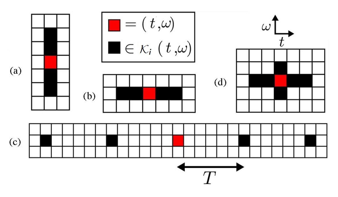
Figure 2: Illustration of several possible kernels [17], (a) for percussive sources, (b) for harmonic sources, (c) for repetitive elements and (d) for smoothly varying sources (e.g. vocal).

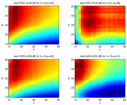
Figure 3: Comparison of the separation quality, measured in terms of RQF, SIR, SDR, SAR [25], as a function of $h$ and $w$, the dimensions of the separation kernels. We considered a musical piece made of 2 sources (voice/drums). A darker red color corresponds to a better separation quality.

As a kernel aims at modeling the vicinity at each point of a time-frequency representation, several typical kernels can be extracted from the literature as presented in Fig. 2. HPSS methods using median filtering [19, 33] can use: (a)+(b). Algorithms such as the REPET algorithm [18, 34], which can separate vocal from accompaniment uses: (c)+(d). These methods use the repetition rate denoted T in Fig. 2, corresponding to the music tempo. For a musical piece T can be constant such as proposed in [18] or time-varying (adaptive) as in [33].

Another question is how to choose the size of a kernel in order to optimize the separation quality? An empirical answer provided by grid search is illustrated in Fig. 3 which shows the best choice for $h$ and $w$, to maximize the separation quality measures (RQF, SIR, SDR, SAR). For this experiment the STFT of a signal sampled at $F_{s}=22.05$ kHz is computed using a Hann window of length $N=2048$ samples ($\approx$92 ms) and an overlap ratio between adjacent frames equal to $\frac{3}{4}$. The separation is obtained using two distinct kernels (cf. Fig. 2 (a)+(b)), to provide 2 sources from a mixture made of a singing voice signal and drums. In this experiment, the best SIR equal to 18.23 dB is obtained with $h=21$ and $w=35$. This is an excellent separation quality in comparison with the oracle BASS method used in Fig. 1. RQF, SDR and SAR related to signal quality, are also satisfying but not optimal.

2.4.2 Towards a training method for supervised KAM-based source separation

To the best of our knowledges, no dedicated method exists to automatically define the best source-specific kernel to use through a KAM-based BASS method. Hence, a classical approach consists of an empirical choice of a predefined typical kernel and of its size. To this end, we propose a new method depicted by Algorithm 5, which provides a source-specific kernel $\mathcal{K}^{b}_{i}\in\{0,1\}^{h\times w}$ associated to the source $i$. The main idea consists in modeling the vicinity of each time-frequency point through an averaged neighborhood map obtained after visiting each coordinate of a source spectrogram. The resulting kernel denoted $\mathcal{K}_{i}\in\mathbb{R}^{h\times w}$ is then binarized in order to be directly used by the KAM method, through a user-defined threshold $\Gamma$ such as:

$$\mathcal{K}^{b}_{i}[c,l]=\begin{cases}1&\text{if ~{}}\mathcal{K}_{i}[c,l]>\Gamma\\ 0&\text{otherwise}\end{cases}.$$ (7)

Our new method based on customized kernels (KAM-CUST) is applied on musical signals in Fig. 5. The results clearly illustrate the different trained source-specific kernels between singing voice, keyboard/synthesizer and drums as in Fig. 2.

Data: $S_{i}$: a source STFT

Result: $\mathcal{K}_{i}\in\mathbb{R}^{h\times w}$, $h$ and $w$ being odd integers.

$K_{j}[c,l]\leftarrow 0$, $\forall c\in[1,w]$, $\forall l\in[1,h]$, and $\forall j\in[1,TF]$

$p_{j}\leftarrow 0,\forall j\in[1,TF]$

$j\leftarrow 1$

for $n\leftarrow$ $1$ to $T$ and $m\leftarrow$ $1$ to $F$ do

       $K_{j}\leftarrow\left|S_{j}[n-\frac{c-1}{2}:n+\frac{c-1}{2},m-\frac{h-1}{2}:m+\frac{h-1}{2}]\right|$

       $K_{j}\leftarrow\frac{K_{j}}{||K_{j}||}$

       $p_{j}\leftarrow|S_{i}[n,m]|^{2}$

       $j\leftarrow j+1$

for $c\leftarrow$ $1$ to $w$ and $l\leftarrow$ $1$ to $h$ do

       $\mathcal{K}_{i}[c,l]\leftarrow\frac{\sum_{j=1}^{TF}K_{j}[c,l]p_{j}}{\sum_{j=1}^{TF}p_{j}}$

Algorithm 5 KAM training algorithm¹.

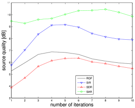
(a) voice

(b) keyboard/synthesizer

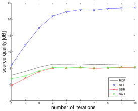
(c) drums

Figure 4: Separation quality using trained kernels on a mixture made of 3 sources as a function of the number of iterations $N_{\text{iter}}$.

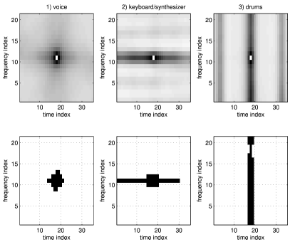
Figure 5: Kernels provided by Algorithm 5 with $\Gamma=0.54$, $h=21$, $w=35$, applied on a mixture of 3 sources: 1) singing voice, 2) keyboard/synthesizer and 3) drums. The first row corresponds to $\mathcal{K}_{i}$ and the second one to $\mathcal{K}^{b}_{i}$.

Table 1: Separation of a mixture made of 3 sources using different KAM configurations.

​ ​ ​

Source	RQF (dB)	SIR (dB)	SDR (dB)	SAR (dB)
voice	6.88	9.12	6.14	9.68
keyboard	2.31	8.36	-1.45	-0.38
drums	6.26	20.98	5.12	5.27

(a) new proposed (KAM-CUST) semi-blind approach using the 3 trained kernels in Fig. 5 ($h=21$, $w=35$, $N_{\text{iter}}=4$, $\alpha=2$)

Source	RQF (dB)	SIR (dB)	SDR (dB)	SAR (dB)
voice	3.16	10.33	0.30	-1.14
keyboard	0.89	4.67	-1.4	1.10
drums	-3.20	3.01	-3.36	-0.47

(b) KAM method using REPET kernels [34, 20] combined with HPSS[19].

Source	RQF (dB)	SIR (dB)	SDR (dB)	SAR (dB)
voice.	4.76	8.06	3.33	5.74
keyb.+drums	1.09	4.04	-2.94	-0.52

(c) KAM method using REPET kernels [34, 20], without HPSS

To show the efficiency of this training method, we apply Algorithm 5 on each isolated component of the same mixture as before made of 3 sources (voice, keyboard/synthesizer and drums) sampled at $F_{s}=22.05$ kHz. The resulting trained kernels displayed in Fig. 5 are then used in combination with Algorithm 4 for KAM-based BASS. In this experiment, we compare the separation results obtained by our proposal (KAM-CUST) with $h=21$, $w=35$, $N_{\text{iter}}=4$, $\alpha=2$ (cf. Table 1 (a)), with the results provided by the KAM-REPET algorithm as implemented by Liutkus [34, 20] (cf. Table 1 (c)) and when KAM-REPET is combined with the HPSS method [19] in order to obtain 3 sources (cf. Table 1 (b)).

The results show that the KAM method combined with trained kernels can significantly outperforms others state-of-the-art methods, particularity in terms of RQF, SIR. Our method also obtains acceptable SDR and SAR (above 5 dB except for the keyboard recovered signal). On the other side, the best SIR result (characterized by a better source isolation) for the extracted singing voice signal, is provided by the combination of the REPET with the HPSS method. However, this approach obtains a poor SDR and SAR results and a lower RQF than using our proposal. Hence, low SDR and low SAR correspond to a poor perceptual audio signal quality where the original signal is altered by undesired artifacts (i.e. undesired sound effects and additive noise).

The impact of the number of iterations $N_{\text{iter}}$ using KAM-CUST is investigated in Fig. 4 which shows that the best RQF for the extracted singing voice can be reached for $N_{\text{iter}}=4$. A higher value of $N_{\text{iter}}$ increases the computation time and can improve the SIR of the accompaniment (which corresponds to a better separation), however it can also add more distortion and artifacts as shown by the SDR and SAR curves which decrease when $N_{\text{iter}}>4$ for the resulting sources.

3 Singing voice detection

In this section, we propose several approaches to detect at each time instant if a singing voice is active into a polyphonic mixture signal. The proposed framework illustrated by Fig. 6 uses source separation as a preliminary step before applying a singing voice detection. We choose to investigate both the unsupervised approach and the supervised approach which uses trained voice models to help the recognition of signal segments containing voice.

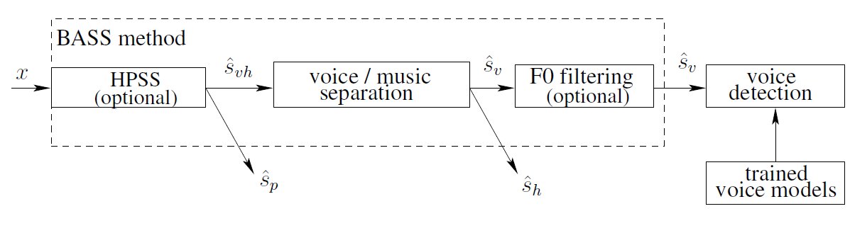
Figure 6: Proposed framework for music source separation and singing voice detection from a polyphonic mixture $x$. HPSS [19] is only used separately when this capability is not included with the BASS method (i.e. KAM-REPET and RPCA). Trained voice models are only used by the supervised approaches.

3.1 Unsupervised Singing Voice Detection

In the unsupervised approach, we do not train specific model for singing voice detection. We only compute a Voice-to-Music Ratio (VTMR) on the estimated signals provided by the BASS methods². The VTMR is a saliency function which is computed on non-silent frames. Thus, two user-defined thresholds are used respectively for silence detection $\Gamma_{\text{s}}$ and for voice detection $\Gamma_{v}$. The voice detection process can thus be described as follows for an input signal mixture $x$.

1. Computation of $\hat{s}_{v}$ and $\hat{s}_{hp}=\hat{s}_{h}+\hat{s}_{p}$, respect to $x=\hat{s}_{v}+\hat{s}_{hp}$, using one of the previously proposed BASS method in Section 2.

2. Application of a band-pass filter on $\hat{s}_{v}$ to allow frequencies in range $[120,3000]$ Hz (adapted to a singing voice bandwidth).

3. Computation of the VTMR on each signal frame of length $N_{v}$ by step $\Delta_{n}$, centered on sample $n$, as:

   $$E[n] =\displaystyle\sum_{k=n-\frac{N_{v}}{2}}^{n+\frac{N_{v}}{2}}|x[k]|^{2}$$

   $$\text{VTMR}[n] =\begin{cases}\frac{\displaystyle\sum_{k=n-\frac{N_{v}}{2}}^{n+\frac{N_{v}}{2}}|\hat{s}_{v}[k]|^{2}}{E[n]},&\text{if~{}}E[n]>\Gamma_{\text{s}}\\ 0&\text{otherwise}\end{cases}$$ (8)

4. The decision to consider if the frame center at time index $n$ contains a singing voice is taken when $\text{VTMR}[n]>\Gamma_{v}$, with $\Gamma_{v}\in[0,1]$. Otherwise, an instrumental or a silent frame is considered.

Hence, in our method we assume that despite errors for estimating the voice signal $\hat{s}_{v}$, its corresponding energy computed on a frame provides sufficiently relevant information to detect the presence of a singing voice in the analyzed mixture. According to this assumption, the selected threshold $\Gamma_{v}$ related to VTMR should be chosen close to 0.5. A lower value is however less restrictive but can provide more false positive results. About the silent detection threshold $\Gamma_{s}$, a low value above zero should be chosen to increase robustness to estimation errors and to avoid a division by zero in Eq. (3). Hopefully, this parameter has shown a weak importance on the voice detection results when it is chosen sufficiently small (e.g. $\Gamma_{s}=10^{-4}$). An illustration of the proposed framework using the KAM-REPET BASS method is presented in Fig. 7 which displays the VTMR (plotted in black) computed for the musical excerpt MusicDelta Punk taken from the MedleyDB dataset [35]. The annotation (also called ref.) is plotted in green and the frames which are detected as containing singing voice correspond to red crosses. In this short excerpt (cf. Fig. 7), results are excellent since the average recall is 0.83, the average precision is 0.63 and the F-measure is equal to 0.72. Further explanations about these evaluation metrics are provided in Section 4.3.

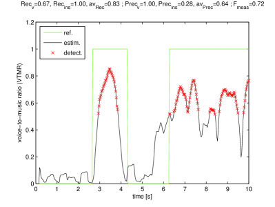
Figure 7: Unsupervised voice detection using KAM-REPET for BASS, applied on the annotated track MusicDelta Punk taken from MedleyDB ($\Gamma_{v}=0.5$).

3.2 HPSS and $F_{0}$ Filtering

In the proposed framework (cf. Fig. 6), any voice/music separation method can be combined with a HPSS method to estimate the percussive part $\hat{s}_{p}$ when it is not directly modeled by the BASS method (i.e. KAM-REPET and RPCA). For this purpose, we simply use KAM with source-specific kernels (a)+(b) presented in Fig. 3. This method is also equivalent to the median filtering approach proposed in [19]. In order to enhance the harmonicity of the voice part, we can apply $F_{0}$ filtering on the estimated singing voice signal $\hat{s}_{v}$. This method previously proposed in [36] for RPCA, consists in estimating at each instant the fundamental frequency $F_{0}$ and to apply a binary mask on a time-frequency representation to isolate the harmonic components (partials) of the predominant $F_{0}$ of $\hat{s}_{v}$, from the background music. In our implementation, the YIN algorithm [37] was used for single $F_{0}$ estimation before the filtering process which considers at each instant, the spectrogram local maxima of the vicinity of each integer multiple of $F_{0}$, as the singing voice partials. Hence, the residual part (not recognized as the partials) is removed from $\hat{s}_{v}$ and added to $\hat{s}_{h}$ (the harmonic instrumental accompaniment). In our experiment, $F_{0}$ Filtering was only combined with RPCA to provide a slight improvement of the original method.

3.3 Supervised Singing Voice Detection

3.3.1 Method description

This technique uses a machine learning framework which remains intensively studied in the literature [38, 39, 23]. It consists in using annotated datasets to train a classification method to automatically predict if a signal fragment of a polyphonic music contains singing voice. Here, we propose to investigate two approaches:

• the “classical” supervised approach which applies singing voice detection without source separation (i.e. directly on the mixture $x$),

• the supervised BASS approach which applies singing voice detection on the isolated signal associated to voice provided by a BASS method (i.e. $\hat{s}_{v}$).

For the classification, each signal is represented by a set of features. In this study, we investigate separately the following descriptors: Mel Frequency Cepstral Coefficients (MFCC) of sources signals as proposed in [38], trained KAM kernels $\mathcal{K}_{i}$ provided by Algorithm 5, Timbre ToolBox (TTB) [40] features and coefficients of the Scattering Transform (SCT) [41]. In order to reduce overfitting, we use the Inertia Ratio Maximization using Features Space Projection (IRMFSP) algorithm [42] as a features selection method.

During the training step, an annotated dataset is used to model the singing voice segments and the instrumental music segments. Hence, we obtain 3 distinct models:

• when isolated voice and music signals are available (i.e. MIR1K and MedleyDB), they are used to obtain respectively the models $\mu_{v}$ and $\mu_{m}$.

• when a singing voice is active over a music background, (i.e. for all datasets) a model $\mu_{vm}$ is obtained.

During the recognition (testing) step, a trained classification method is then applied on signal fragments to detect singing voice activity.

3.3.2 Features selection for voice detection

In order to assess the efficiency of the proposed features for the supervised method, we computed for the Jamendo dataset [38], a 3-fold cross validation (with randomly defined folds) using the Support Vector Machines (SVM) method with a radial basis kernel, combined with the IRMFSP method [42] to obtain the top-100 best features to discriminate between vocal and musical signal frames. In this experiment, each music except is represented by concatenated features vectors computed on each 371 ms-long frames (without overlap between adjacent frames). We configure each method such as KAM provides 361 values (using $w=h=19$), MFCCs provide 273 values (13 MFCCS on 21 frames), TTB provides 164 coefficients and SCT provides 866 coefficients. The results measured in terms of F-measure are displayed in Table 2 and shows that SCT is the most important feature which outperforms the other ones. Despite KAM shows its capabilities for source separation, it however provides the poorest results but close to MFCCs results, for singing voice detection. The best results are obtained thanks to SCT which should be used in combination with the TTB.

Table 2: Investigation of the most efficient features for singing voice detection on the Jamendo dataset.

KAM	MFCC	TTB	SCT	$F_{\text{meas}}$
x				.75
	x			.80
		x		.82
			x	.89
x	x			.82
x		x		.83
x			x	.88
	x	x		.85
	x		x	.89
		x	x	.89
x	x	x		.84
x	x		x	.88
x		x	x	.88
	x	x	x	.89
x	x	x	x	.89

4 Numerical results

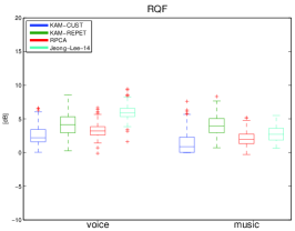
(a) RQF

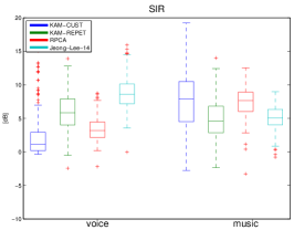
(b) SIR

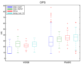
(c) Overall-Perceptual Score (percents)

Figure 8: Objective and perceptual BASS quality results comparison on the test-fold of the MIR1K dataset.

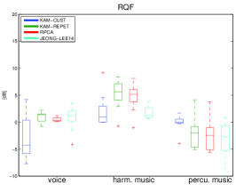
(a) RQF

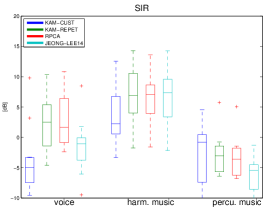
(b) SIR

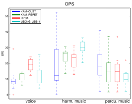
(c) Overall-Perceptual Score (percents)

Figure 9: Objective and perceptual BASS quality results comparison on the test-fold of the MedleyDB dataset.

4.1 Datasets

In our experiments, we use several common datasets allowing evaluation for source separation (MedleyDB, MIR1K) and singing voice detection from a polyphonic mixture. About singing voice detection, each dataset is split in several folds corresponding to training and test folds which are both used by the evaluated supervised methods. The unsupervised methods only use the test fold. Hence, we used 3 datasets.

• Jamendo [38] contains creative commons music track with singing voice annotations. The whole dataset contains 93 tracks where 61 correspond to the training set and 16 tracks are used respectively for the test and the validation. Since the separated tracks of each source are not available, this dataset is only used for singing voice detection.

• MedleyDB [35] contains 122 music pieces of different styles, available with the separate multi-track instruments (60 with and 62 without singing voice). This, allows to build a flat instantaneous single-channel mixture mix to fit the signal model proposed by Eq. (1). We have made a split on this dataset which preserve the ratio of voiced-unvoiced musical tracks while ensuring that each artist is only present once on each fold. Finally, the training dataset contains 62 tracks, the test set 36 tracks and the validation 24 tracks. For the source separation and the singing voice detection tasks, we only focus on 50 music tracks containing singing voice.

• MIR1K [43] contains 1000 musical excerpts recorded during karaoke sessions with 19 different non-professional singers. For each track the voice and the accompaniment is available. We propose to split this dataset to obtain 828 excerpts for the training and 172 excerpts for the test set (containing only the singers ‘HeyCat’ and ‘Amy’).

4.2 Blind Source Separation

Now, we compare the source separation performance respectively obtained on MIR1K (voice/music) and on MedleyDB (voice/music/drums) datasets using the investigated methods: KAM-REPET, KAM-CUST, RPCA and Jeong-Lee methods. For each musical track, the isolated source signals are used to construct mixtures through Eq. (1) on which the BASS methods are applied. Isolated signal are also used as references to compute the source separation quality measures. Each analyzed excerpt is sampled at $F_{s}=22.05$ kHz and each method is configured to provide the best results according to Section 2:

• KAM-REPET is a variant of the original REPET algorithm proposed by A. Liutkus in [20] which uses a local time-varying tempo estimator to separate the leading melody from the repetitive musical background. To obtain 3 sources (on MedleyDB), this method is combined with the HPSS method [19] with $h=w=19$ (as preprocessing) to separate the percussive part.

• KAM-CUST is the new proposed method (cf. Section 2.4) based on the KAM framework using a supervised kernel training step. In our experiment, we directly train the kernels on the isolated reference signals used to create the mixtures. Trained kernels are configured such as $h=w=19$.

• RPCA corresponds to our implementation of this method with $\lambda=\frac{2}{\sqrt{\max(F,T)}}$, $\mu=10\lambda$ and $N_{\text{iter}}=1000$. As for the KAM-REPET method, this approach can be combined with the HPSS [19] and $F_{0}$-filtering to provide 2 or 3 sources when it is required.

• Jeong-Lee-14 corresponds to our implementation of Algorithm 2 with $\alpha\!=\!1/4$, $\phi\!=\!1/40$, $N_{\text{iter}}\!=\!200$, $\gamma\!=\!1/4$.

The results displayed in Fig. 8 (MIR1K) and in Fig. 9 (MedleyDB) use the boxplot representation [44] and measure the BASS quality in terms of RQF, SIR and Overall Perceptual Score (OPS) provided by BssEval² [25, 45]. Jeong-Lee-14 and KAM-REPET obtain the best SIR results on MIR1K for separating the voice without drums separation (cf. Fig. 8). Interestingly, Jeong-Lee-14 can significantly outperforms other methods for voice separation on MIR1K, but it can also obtain the worst results on MedleyDB. From another side, RPCA and KAM-REPET obtain the best SIR results for separating the voice in combination with drums separation (cf. Fig. 9) on MedleyDB. Unfortunately, KAM-CUST fails to separate the voice properly. However it can obtain the best results for accompaniment separation. This can be explained by the variability of a singing voice spectrogram which is not sufficiently modeled by our training Algorithm. At the contrary, better results are provided for the accompaniment which has a more stable time-frequency structure. This can also be explained by MedleyDB for which several references signal are not well isolated. This produces errors in the trained kernels which are used by KAM-CUST.

4.3 Singing voice detection

Each evaluated method is configured to detect the presence of a singing voice activity on each signal frame of length 371.5 ms (8192 samples at $F_{s}=$22.05 kHz) by steps of 30 ms. In order to compare the performance of the different proposed singing voice detection methods, we use the recall (Rec), precision (Prec) and F-measure ($F_{\text{meas}}$) metrics which are commonly used to assess Music Information Retrieval (MIR) systems [46]. Rec (resp. Prec) is defined for each class (i.e. voice ($v$) and music ($hp$)) and is averaged among classes to obtain the $\text{av}_{\text{Rec}}$ (resp. $\text{av}_{\text{Prec}}$). The F-measure is thus obtained by computing the harmonic average between $\text{av}_{\text{Rec}}$ and $\text{av}_{\text{Prec}}$ such as:

$$F_{\text{meas}}=2\frac{\text{av}_{\text{Rec}}\cdot\text{av}_{\text{Prec}}}{\text{av}_{\text{Rec}}+\text{av}_{\text{Prec}}}.$$ (9)

4.3.1 Unsupervised singing voice detection

In this experiment we respectively apply the 4 investigated BASS methods described in Section 2 and 4.2 to estimate the voice source and the musical parts before applying the unsupervised approach described in Section 3.1. Our results obtained on the MedleyDB and the MIR1K datasets are presented in Tables 10(b) (a) and (b). The results are compared to those provided by the oracle which corresponds to the Algorithm 1 which apply a Wiener filter with $\alpha=2$ and where the isolated reference signals are assumed known. Interestingly, the best results are reached using the KAM-REPET method without HPSS on MedleyDB and with Jeong-Lee-14 on MIR1K with a F-measure above 0.60.

4.3.2 BASS + supervised singing voice detection

In this experiment, we combine a BASS method with the best SVM-based proposed supervised singing voice detection method as investigated in Table. 2 (i.e. using TTB + SCT). According to Tables 10(d) (a) and (b), combining BASS with supervised singing voice detection can slightly improve the precision of detection in comparison with the unsupervised approach (in particular KAM-REPET and KAM-CUST). However, this approach shows a limited interest of BASS for supervised singing voice detection, in comparison with other approaches. In fact, this approach does not allow to overcome the best score reached through the unsupervised method, in particular the maximal recall reached for MedleyDB which remains equal to 0.59. A solution not investigated here could be to train models specific to the results provided by a BASS, but without the insurance to obtain better results than without using BASS.

4.3.3 Supervised singing voice detection: comparison with CNN

Finally, we compare all the proposed approaches (unsupervised and supervised) in terms of singing voice detection accuracy with an implementation of a recent state-of-the-art method [23] based on CNN. The results obtained on a single dataset and after merging two datasets, are respectively displayed in Tables. 10(f) (a) and (b). For the sake of clarity, we only compare the average recall results which is the most important metric. Table 10(f) (b) considers two experimental cases. The Self-DB case considers two datasets as a single dataset by merging their respective training parts (e.g. MIR1K-train + JAMENDO-train) and by merging their test parts (e.g. MIR1K-test + JAMENDO-test). The cross-DB case uses two merged datasets for the training step (e.g. MIR1K-train + JAMENDO-train) and uses the third dataset for testing the singing voice detection (i.e. MedleyDB-test). Results show that the CNN-based method outperforms the proposed unsupervised and the supervised methods when it is applied on single datasets (cf. (a) and seld-DB (b)). However, the unsupervised approach can beat CNN in cross-DB (b) case. This is visible for the MIR1K where the best unsupervised methods (RPCA and Jeong-Lee-14) obtain a recall equal to 0.68 when the CNN-based method is trained on Jamendo+MedleyDB only 0.65. This result shows that an unsupervised approach can also be of interest to avoid overfitting or when no training dataset is available. Moreover, our proposed supervised methods can obtain comparable results to CNN in the cross-DB case except for singing voice detection applied on MIR1K.

Table 3: Unsupervised voice detection results using BASS (bold values denotes best results except for Oracle).

	av. Rec.	av. Prec.	F-meas
Oracle	0.71	0.66	0.68
KAM-REPET	0.59	0.68	0.63
KAM-REPET + HPSS	0.54	0.69	0.60
KAM-CUST	0.50	0.62	0.55
RPCA	0.52	0.76	0.61
RPCA + HPSS	0.53	0.75	0.62
Jeong-Lee-14	0.50	0.65	0.56

(a) with and without drums separation on the MedleyDB dataset

	av. Rec.	av. Prec.	F-meas
Oracle	0.82	0.72	0.76
KAM-REPET	0.65	0.75	0.69
KAM-CUST	0.57	0.55	0.55
RPCA	0.68	0.61	0.64
Jeong-Lee-14	0.68	0.78	0.72

(b) without drums separation applied on the MIR1K dataset

Table 4: BASS combined with supervised singing voice detection results (bold values denotes best results except for Oracle).

	av. Rec.	av. Prec.	F-meas
Oracle	0.71	0.68	0.69
KAM-REPET + HPSS	0.52	0.76	0.61
KAM-CUST	0.59	0.64	0.61
RPCA + HPSS	0.55	0.69	0.61
Jeong-Lee-14	0.49	0.64	0.55

(c) with drums separation applied on the MedleyDB dataset

	av. Rec.	av. Prec.	F-meas
Oracle	0.67	0.61	0.63
KAM-REPET	0.60	0.70	0.64
KAM-CUST	0.52	0.62	0.56
RPCA	0.55	0.74	0.63
Jeong-Lee-14	0.51	0.72	0.59

(d) without drums separation applied on the MIR1K dataset

Table 5: Comparison of the proposed methods with [23] measured in terms of average recall for singing voice detection.

Dataset	Best unsupervised	SVM (MFCC+SCT)	CNN
Jamendo	0.58	0.81	0.86
MIR1K	0.68	0.77	0.9
MedleyDB	0.59	0.79	0.86

(e) evaluation on each dataset

Training datasets	SVM (MFCC+SCT)		CNN
	self-DB	cross-DB	self-DB	cross-DB
Jamendo + MIR1K	0.81	0.73	0.89	0.75
Jamendo + MedleyDB	0.80	0.59	0.86	0.65
MedleyDB + MIR1K	0.80	0.76	0.84	0.77

(f) evaluation on merged datasets

5 Conclusion

We have presented recent developments for blind single-channel audio source separation methods, which use morphological filtering of the mixture spectrogram. These methods were compared together for source separation and using our new framework for singing voice detection which uses BASS as a preprocessing step. We have also proposed a new contribution to extend the KAM framework to automatically design kernels which fits any given audio source. Our results show that our proposed KAM-CUST method is promising and can obtain better results than KAM-REPET for blind source separation. However, our training algorithm is sensitive and should be further investigated to provide discriminative source-specific kernels. Moreover, we have shown that the unsupervised approach remains of interest for singing voice detection in comparison with more efficient method such as [23] based on CNN. In fact, the weakness of supervised approaches can become visible when large databases are processed or when a few annotated examples are available. Hence, this study paves the way of a future investigation of the KAM framework in order to efficiently design source-specific kernels which can be used both for source separation or for singing voice detection. Future works will consider new practical applications of the proposed methods while improving the robustness of the new proposed KAM training algorithm.

References

- [1] P. Comon and C. Jutten, Handbook of Blind Source Separation: Independent component analysis and applications. Academic press, 2010.
- [2] P. Bofill and M.Zibulevski, “Underdetermined blind source separation,” Signal Processing, vol. 81, no. 11, pp. 2353–2362, 2001.
- [3] J. Idier, Bayesian approach to inverse problems. John Wiley & Sons, 2013.
- [4] E. Vincent, H. Sawada, P. Bofill, S. Makino, and J. P. Rosca, “First stereo audio source separation evaluation campaign: data, algorithms and results,” in International Conference on Independent Component Analysis and Signal Separation. Springer, 2007, pp. 552–559.
- [5] F. R. Stöter, A. Liutkus, R. Badeau, B. Edler, and P. Magron, “Common fate model for unison source separation,” in Proc. IEEE International Conference on Acoust., Speech and Signal Process. (ICASSP), Mar. 2016, pp. 126–130.
- [6] T. Barker and T. Virtanen, “Blind separation of audio mixtures through nonnegative tensor factorization of modulation spectrograms,” IEEE/ACM Trans. on Audio, Speech, and Language Processing, vol. 24, no. 12, pp. 2377–2389, Dec. 2016.
- [7] E. Creager, N. D. Stein, R. Badeau, and P. Depalle, “Nonnegative tensor factorization with frequency modulation cues for blind audio source separation,” in Proc. of the International Society for Music Information Retrieval Conference (ISMIR), New York, NY, United States, Aug. 2016.
- [8] A. Jourjine, S. Rickard, and O. Yilmaz, “Blind separation of disjoint orthogonal signals: demixing n sources from 2 mixtures,” in Proc. IEEE International Conference on Acoust., Speech and Signal Process. (ICASSP), Istanbul, Turquie, Jun. 2000, pp. 2985–2988.
- [9] A. S. Bregman, Auditory scene analysis. MIT Press: Cambridge, MA, 1990.
- [10] E. Creager, “Musical source separation by coherent frequency modulation cues,” Master’s thesis, Department of Music Research, Schulich School of Music, McGill University, Dec. 2015.
- [11] D. Fourer, F. Auger, and G. Peeters, “Estimation locale des modulations AM/FM: applications à la modélisation sinusoïdale audio et à la séparation de sources aveugle,” in Proc. GRETSI’17, France, Aug. 2017.
- [12] D. Fourer and S. Marchand, “Informed spectral analysis: audio signal parameters estimation using side information,” EURASIP Journal on Advances in Signal Processing, vol. 2013, no. 1, p. 178, Dec. 2013.
- [13] B. Lehner and G. Widmer, “Monaural blind source separation in the context of vocal detection,” in Proc. of the International Society for Music Information Retrieval Conference (ISMIR), 2015, pp. 309–315.
- [14] I.-Y. Jeong and K. Lee, “Vocal separation from monaural music using temporal/spectral continuity and sparsity constraints,” IEEE Signal Process. Lett., vol. 21, no. 10, pp. 1197–1200, 2014.
- [15] E. J. Candès, X. Li, Y. Ma, and J. Wright, “Robust principal component analysis?” Journal of the ACM (JACM), vol. 58, no. 3, p. 11, 2011.
- [16] P.-S. Huang, S. D. Chen, P. Smaragdis, and M. Hasegawa-Johnson, “Singing-voice separation from monaural recordings using robust principal component analysis,” in Proc. IEEE International Conference on Acoust., Speech and Signal Process. (ICASSP), 2012, pp. 57–60.
- [17] A. Liutkus, D. Fitzgerald, Z. Rafii, B. Pardo, and L. Daudet, “Kernel additive models for source separation,” IEEE Trans. Signal Process., vol. 62, no. 16, pp. 4298–4310, Aug. 2014.
- [18] Z. Rafii and B. Pardo, “Repeating pattern extraction technique (REPET): A simple method for music/voice separation,” IEEE/ACM Trans. on Audio, Speech, and Language Processing, vol. 21, no. 1, pp. 73–84, 2013.
- [19] D. Fitzgerald, “Harmonic/percussive separation using median filtering,” in Proc. Digital Audio Effects Conference (DAFx-10). Dublin Institute of Technology, 2010.
- [20] A. Liutkus, D. Fitzgerald, and Z. Rafii, “Scalable audio separation with light kernel additive modelling,” in Proc. IEEE International Conference on Acoust., Speech and Signal Process. (ICASSP), Brisbane, Australia, Apr. 2015, pp. 76–80.
- [21] H.-G. Kim and J. Y. Kim, “Music/voice separation based on kernel back-fitting using weighted -order MMSE estimation,” ETRI Journal, vol. 38, no. 3, pp. 510–517, Jun. 2016.
- [22] H. Cho, J. Lee, and H.-G. Kim, “Singing voice separation from monaural music based on kernel back-fitting using beta-order spectral amplitude estimatio,” in Proc. of the International Society for Music Information Retrieval Conference (ISMIR), 2015, pp. 639–644.
- [23] J. Schlüter, “Learning to pinpoint singing voice from weakly labeled examples,” in Proc. of the International Society for Music Information Retrieval Conference (ISMIR), 2016, pp. 44–50.
- [24] P. Flandrin, Time-Frequency/Time-Scale analysis. Acad. Press, 1998.
- [25] E. Vincent, R. Gribonval, and C. Févotte, “Performance measurement in blind audio source separation,” IEEE/ACM Trans. on Audio, Speech, and Language Processing, vol. 14, no. 4, pp. 1462–1469, Jul. 2006.
- [26] V. Emiya, E. Vincent, N. Harlander, and V. Hohmann, “Subjective and objective quality assessment of audio source separation,” IEEE/ACM Trans. on Audio, Speech, and Language Processing, vol. 19, no. 7, pp. 2046–2057, 2011.
- [27] M. Fontaine, A. Liutkus, L. Girin, and R. Badeau, “Explaining the parameterized wiener filter with alpha-stable processes,” in Proc. IEEE Workshop on Applications of Signal Processing to Audio and Acoustics (WASPAA), Oct. 2017.
- [28] M. Najim, Modeling, estimation and optimal filtration in signal processing. John Wiley & Sons, 2010, vol. 25.
- [29] D. Fourer, F. Auger, and P. Flandrin, “Recursive versions of the Levenberg-Marquardt reassigned spectrogram and of the synchrosqueezed STFT,” in Proc. IEEE International Conference on Acoust., Speech and Signal Process. (ICASSP), Mar. 2016, pp. 4880–4884.
- [30] L. I. Rudin, S. Osher, and E. Fatemi, “Nonlinear total variation based noise removal algorithms,” Physica D: Nonlinear Phenomena, vol. 60, no. 1-4, pp. 259–268, 1992.
- [31] Z. Lin, M. Chen, L. Wu, and Y. Ma, “The augmented lagrange multiplier method for exact recovery of a corrupted low-rank matrices,” in Mathematical Programming, 2009.
- [32] W. S. Cleveland and S. J. Devlin, “Locally weighted regression: an approach to regression analysis by local fitting,” Journal of the American statistical association, vol. 83, no. 403, pp. 596–610, 1988.
- [33] D. FitzGerald, A. Liukus, Z. Rafii, B. Pardo, and L. Daudet, “Harmonic/percussive separation using kernel additive modelling,” in 25th IET Irish Signals Systems Conference 2014 and 2014 China-Ireland International Conference on Information and Communications Technologies (ISSC 2014/CIICT 2014), Jun. 2014, pp. 35–40.
- [34] A. Liutkus, Z. Rafii, R. Badeau, B. Pardo, and G. Richard, “Adaptive filtering for music/voice separation exploiting the repeating musical structure,” in Proc. IEEE International Conference on Acoust., Speech and Signal Process. (ICASSP), Kyoto, Japan, 2012, pp. 53–56.
- [35] R. Bittner, J. Salamon, M. Tierney, M. Mauch, C. Cannam, and J. P. Bello, “MedleyDB: A multitrack dataset for annotation-intensive MIR research,” in Proc. of the International Society for Music Information Retrieval Conference (ISMIR), Taipei, Taiwan, Oct. 2014.
- [36] Y. Ikemiya, K. Itoyama, and K. Yoshii, “Singing voice separation and vocal f0 estimation based on mutual combination of robust principal component analysis and subharmonic summation,” IEEE/ACM Trans. on Audio, Speech, and Language Processing, vol. 24, no. 11, pp. 2084–2095, Nov. 2016.
- [37] A. De Cheveigné and H. Kawahara, “Yin, a fundamental frequency estimator for speech and music,” The Journal of the Acoustical Society of America, vol. 111, no. 4, pp. 1917–1930, 2002.
- [38] M. Ramona, G. Richard, and B. David, “Vocal detection in music with support vector machines,” in Proc. IEEE International Conference on Acoust., Speech and Signal Process. (ICASSP), Mar. 2008, pp. 1885–1888.
- [39] L. Regnier and G. Peeters, “Singing voice detection in music tracks using direct voice vibrato detection,” in Proc. IEEE International Conference on Acoust., Speech and Signal Process. (ICASSP), 2009, pp. 1685–1688.
- [40] G. Peeters, B. Giordano, P. Susini, N. Misdariis, and S. McAdams, “The timbre toolbox: Audio descriptors of musical signals,” Journal of Acoustic Society of America (JASA), vol. 5, no. 130, pp. 2902–2916, Nov. 2011.
- [41] J. Andén and S. Mallat, “Multiscale scattering for audio classification.” in Proc. of the International Society for Music Information Retrieval Conference (ISMIR), 2011, pp. 657–662.
- [42] G. Peeters, “Automatic classification of large musical instrument databases using hierarchical classifiers with inertia ratio maximization,” in 115th AES Convention, NY, USA, Oct. 2003.
- [43] C.-L. Hsu and J.-S. R. Jang, “On the improvement of singing voice separation for monaural recordings using the MIR-1K dataset,” IEEE/ACM Trans. on Audio, Speech, and Language Processing, vol. 18, no. 2, pp. 310–319, 2010.
- [44] Y. Benjamini, “Opening the box of a boxplot,” The American Statistician, vol. 42, no. 4, pp. 257–262, 1988.
- [45] V. Emiya, E. Vincent, N. Harlander, and V. Hohmann, “Subjective and objective quality assessment of audio source separation,” IEEE/ACM Trans. on Audio, Speech, and Language Processing, vol. 19, no. 7, pp. 2046–2057, 2011.
- [46] M. Bay, A. F. Ehmann, and J. S. Downie, “Evaluation of multiple-f0 estimation and tracking systems.” in Proc. of the International Society for Music Information Retrieval Conference (ISMIR), 2009, pp. 315–320.