Visual Object Tracking: The Initialisation Problem

Abstract

Model initialisation is an important component of object tracking. Tracking algorithms are generally provided with the first frame of a sequence and a bounding box (BB) indicating the location of the object. This BB may contain a large number of background pixels in addition to the object and can lead to parts-based tracking algorithms initialising their object models in background regions of the BB. In this paper, we tackle this as a missing labels problem, marking pixels sufficiently away from the BB as belonging to the background and learning the labels of the unknown pixels. Three techniques, One-Class SVM (OC-SVM), Sampled-Based Background Model (SBBM) (a novel background model based on pixel samples), and Learning Based Digital Matting (LBDM), are adapted to the problem. These are evaluated with leave-one-video-out cross-validation on the VOT2016 tracking benchmark. Our evaluation shows both OC-SVMs and SBBM are capable of providing a good level of segmentation accuracy but are too parameter-dependent to be used in real-world scenarios. We show that LBDM achieves significantly increased performance with parameters selected by cross validation and we show that it is robust to parameter variation.

I Introduction

Object tracking in video is an important topic within computer vision, with a wide range of applications, such as surveillance, activity analysis, robot vision, and human-computer interfaces. Recent benchmarks for this problem have been created to evaluate algorithms that are designed for single-object, short-term, and model-free, tracking [1, 2]. The model-free aspect of the problem is particularly challenging as this means that a tracker has no prior knowledge of the characteristics (such as colour, shape, and texture) of the object. In common with real world applications, tracking algorithms are only provided with the first frame of a video, along with a bounding box (BB) that indicates which region of the image contains the object. Typically up to 30% of this region is comprised of pixels not belonging to the object, i.e. background [2]. Initialising tracking algorithms with background instead of foreground can be severely deleterious to their performance, so in this paper we examine the initialisation problem of locating the object to be tracked within the given BB.

Tracking algorithms generally fall into two categories: those that track the entire object via some holistic model which captures the appearance of the object and potentially its surroundings in some way [3, 4, 5], and parts-based models [6, 7, 8]. These latter decompose an object into a loosely connected set of parts, each with its own visual model, allowing for better modelling of objects which undergo geometrical deformations and changes in appearance [7]. Incorrect initialisation of parts-based trackers can lead to multiple parts being initialised to regions, within the BB, that do not belong to the object. This can cause parts to drift away from the object during tracking, as the object, but not its background, moves.

This problem is typically dealt with in two ad hoc ways: attempting to select regions of the BB to track that are highly likely to belong to the object; and also removing parts from an object’s model that exhibit signs of poor performance, reinitialising these parts as required [6]. Both of these methods attempt to ascertain the object’s exact location based on the limited information available to them, knowing only where the object approximately resides, such as inside the BB during initialisation. However, it is not known which pixels within, and close to, this region belong to the object and which belong to its background. We refer to the problem of determining which pixels, given an approximate location of the object, belong to the object and which do not, as the Initialisation Problem.

Recently, some parts-based techniques have attempted to address the initialisation problem in various ways. Several methods [7, 8, 9] distribute their parts uniformly over the BB and employ aggressive update schemes to identify patch drift. Other methods, e.g. [10, 11], employ oversegmentation techniques, such as superpixeling, to mark all pixels belonging to a superpixel that crosses the BB as not belonging to the object. Others attempt to select regions of the BB with desirable attributes for the particular tracking algorithm being used. These include selecting areas likely to have good optical flow estimation [12] and areas with good image alignment properties [6].

In this paper we address the initialisation problem by treating it as a missing labels problem, as we can be sure that pixels sufficiently outside the BB do not belong to the object. The problem is challenging, however, because BBs are generally small and the object itself may be quite similar in appearance to the background. In addition, the object to be tracked may extend outside the given BB [13]. For example, in order to reduce the number of background pixels within a BB, the outstretched limb of a person to be tracked might be excluded from the initialising BB. This means that the distance away from a BB where pixels are certainly background may be different for each segmentation. We note too that distance from the BB is not a guarantee that a pixel or region’s appearance is not similar to the appearance of the object to be tracked; a common example is tracking a particular face in a crowd.

We evaluate the performance of three techniques: the first two, One-Class SVM (OC-SVM) and a novel Sample-Based Background Model (SBBM), treat the problem as a one-class classification problem. They attempt to learn the characteristics of the background regions of the image; pixels within the BB are then compared to the background model to determine object pixels. The third technique is an adapted solution to the image matting problem. This models each pixel in the image as comprising proportions of both foreground and background colour, aiming to to learn these proportions. The performance of these three techniques is evaluated by assessing their segmentation on the Visual Object Tracking 2016, VOT2016, dataset [2]. We discuss their strengths and weaknesses and investigate the robustness to parameter settings of the learned matting method.

The rest of the paper is organised as follows. In Section II we formulate the initialisation problem and present the three techniques to be empirically compared. The experimental procedure and results are presented in Sections III and IV, and are followed by concluding remarks in Section V.

II Methods

We aim to determine the label $k\in\left\{0,1\right\}$ of each pixel in the image, where the two labels represent belonging to the background of the BB and the object itself, respectively. The image $I$ containing the object consists of a set of pixels indexed by $\Omega=\left\{1,\ldots,n\right\}$, where $n$ is the total number of pixels in the image. Given a subset of these pixels $\Omega_{b}\subset\Omega$ which belong to the background, such that $k_{i}=0\>\forall\>i\in\Omega_{b}$, then the problem can be formulated as learning the correct labels of the unlabelled pixels $\Omega_{u}=\Omega\setminus\Omega_{b}$.

Rather than treating each pixel $i\in\Omega$, or features extracted from them, as a data point, two of the methods we examine use a superpixel representation, which provides a richer description of small, approximately homogeneous, image regions. Superpixeling techniques oversegment the image into perceptually meaningful regions (the pixels in a superpixel are generally uniform in colour and texture), while at the same time retaining the image structure, as superpixels tend to adhere to colour and shape boundaries. Using superpixeling also can also significantly reduce the computational complexity because groups of pixels are represented as a single entity. An image $I$ is therefore comprised of a set of superpixels $\mathcal{S}=\left\{S_{j}\right\}_{j=1}^{{N_{sp}}}$, where $N_{sp}$ is the number of superpixels, and we associate a vector of features $\boldsymbol{\mathbf{x}}_{j}\in\mathbb{R}^{d}$, such as a histogram of its RGB values, with each superpixel.

II-A One-Class SVM

In general, pixels belonging to the object are not known, but a large number of pixels or superpixels may be assumed to belong to the background. We therefore treat the initialisation problem as that of identifying pixels which are significantly different from the background. This can be accomplished by using a one-class SVM (OC-SVM) to estimate the support of the given background pixels.

The goal of an OC-SVM [14] is to learn the hyperplane $\boldsymbol{\mathbf{w}}\in\mathcal{F}$ that produces the maximum separation between the origin and data points $\{\boldsymbol{\mathbf{x}}_{i}\}_{i=1}^{N},\,\boldsymbol{\mathbf{x}}_{i}\in\mathcal{X}$ mapped to a suitable feature space $\mathcal{F}$. It uses an implicit function $\Phi\left(\cdot\right)$ to map the data into a dot product feature space $\Phi$: $\mathcal{X}\mapsto\mathcal{F}$ using a kernel $k\left(\boldsymbol{\mathbf{x}},\boldsymbol{\mathbf{y}}\right)=\langle\Phi\left(\boldsymbol{\mathbf{x}}\right),\Phi\left(\boldsymbol{\mathbf{y}}\right)\rangle$. The radial basis function kernel (Gaussian kernel), $k\left(\boldsymbol{\mathbf{x}},\boldsymbol{\mathbf{y}}\right)=e^{-\gamma\left\lVert\boldsymbol{\mathbf{x}}-\boldsymbol{\mathbf{y}}\right\rVert^{2}}$, is a popular choice, as this guarantees the existence of such a hyperplane [14]. The decision function $f\left(\boldsymbol{\mathbf{x}}\right)=\text{sgn}\left(\boldsymbol{\mathbf{w}}\cdot\Phi\left(\boldsymbol{\mathbf{x}}\right)-\rho\right)$, is used to determine whether an arbitrary input vector $\boldsymbol{\mathbf{x}}$ belongs to the one defined class when $\boldsymbol{\mathbf{w}}\cdot\Phi\left(\boldsymbol{\mathbf{x}}\right)\geq\rho$.

In order to find $\boldsymbol{\mathbf{w}}$ and the threshold $\rho$, the problem can be defined in its primal form:

$$\operatorname*{min}_{\boldsymbol{\mathbf{w}}\in\mathcal{F},\>\boldsymbol{\mathbf{\xi}}\in\mathbb{R}^{N},\>\rho\in\mathbb{R}} \frac{1}{2}\left\lVert\boldsymbol{\mathbf{w}}\right\rVert^{2}-\rho+\frac{1}{\nu N}\sum_{i}\xi_{i}$$ (1)

subject to $$\quad\boldsymbol{\mathbf{w}}\cdot\Phi\left(\boldsymbol{\mathbf{x}}_{i}\right)\geq\rho-\xi_{i},\quad\xi_{i}\geq 0,$$ (2)

where slack variables $\xi_{i}$ allow the corresponding $\boldsymbol{\mathbf{x}}_{i}$ to lie on the other side of the decision boundary, and $\nu\in\left(0,1\right)$ is a regularisation parameter. Conversion to the dual form reveals that the solution can be written as a sparse weighted sum of support vectors and solved by quadratic programming or, more typically, Sequential Minimal Optimisation [15].

The parameter $\nu$ acts both as an upper bound on the fraction of outliers (data points with $f\left(\boldsymbol{\mathbf{x}}\right)<0$) and a lower bound on the fraction of data points used as support vectors. It is worth noting that, for kernels such that $k(\boldsymbol{\mathbf{x}}_{i},\boldsymbol{\mathbf{x}}_{i})=c\>\forall\>\boldsymbol{\mathbf{x}}_{i}\in\mathcal{X}$, where $c$ is some constant, this formulation is equivalent [16] to that of using Support Vectors for Data Description [17], in which the goal is to encapsulate most of the data in a hypersphere in $\mathcal{F}$.

II-A1 Application

In order to use the OC-SVM approach, the image is preprocessed and features extracted in order to train the classifier and identify which regions of the image belong to the object. As illustrated in Fig. 1a, the image $I$ is first cropped to twice the width and height of an axis-aligned BB containing the supplied BB and object. The cropping allows for a sufficient region of the image to be included to train the classifier, while only including areas relatively close, in terms of the object’s size, to the object. The cropped region is then segmented using a variant of the SLIC superpixeling algorithm [18], SLIC0, which produces regular shaped (compact) superpixels (Fig. 1b), while adhering to image boundaries in both textured and non-textured regions of the image.

The main parameter of SLIC0 is the approximate number of superpixels $N_{sp}$ resulting from the segmentation. Following preliminary experiments, we aim to have an average of 50 pixels per superpixel to give a sufficient number of pixels from which to extract features. However, given the varying size of each cropped image, this could result in very few or very many superpixels. Therefore we constrain the number of superpixels to lie in the range $\left[N_{sp}^{-},N_{sp}^{+}\right]$. We use $N_{sp}^{-}=100$ and $N_{sp}^{+}=500$, as these have empirically given reasonable-looking segmentations and are similar to the range used by [10].

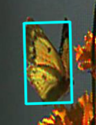
(a)

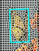
(b)

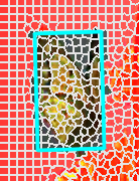
(c)

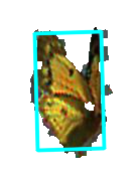
(d)

Figure 1: The OC-SVM pipeline. The image is first cropped (a) and then superpixeled (b). The OC-SVM is trained ($\gamma=2^{-20}$, $\nu=0.3$) using the superpixels considered background in (c), and those with an unknown label (uncoloured) have their class predicted, giving a final predicted object mask (d).

Following segmentation, superpixels that lie wholly outside the BB are labelled as not belonging to the object, such as the red superpixels in Fig. 1c, with the features extracted from these forming the training data. We examine the performance of four alternative feature representations: histograms of RGB or, perceptually uniform, LAB pixel intensities across the superpixel; or the concatenated SIFT [19] or LBP [20] feature vectors resulting from the R, G and B channels at the centroid of the superpixels. Both SIFT and LBP are popular texture-based feature descriptors, with SIFT features extracted based on the region’s gradient magnitude and orientation [19], and LBP features formed based on differences in intensity between a pixel and its surrounding neighbours [20].

The classifier, with its parameters $\gamma$ and $\nu$, representing the kernel’s length-scale and the classifier’s upper bound on the assumed number of outliers in the training set, is subsequently trained on this data. Finally, features extracted from the unknown superpixels, lying wholly or partially within the given BB are classified with the trained OC-SVM. Fig. 1d shows the resulting segmentation.

II-B Sample-Based Background Model

Our sample-based one-class modelling technique is inspired by the background subtraction algorithm of [21]. We represent labelled regions of the image, in this case superpixels, by sets of samples that characterise the colour distribution of these regions. In the same way as described in Section II-A1, the region surrounding the supplied BB is cropped and over-segmented into superpixels (Fig. 2a and 2b). Superpixels lying wholly outside the specified BB are labelled as background (Fig. 2c).

An unlabelled superpixel is compared to the modelled superpixels by evaluating how similar its set of samples is to each of the labelled sets of samples. The unlabelled superpixel is classified as either belonging to the labelled region (background) of the image if it is sufficiently similar to any of the labelled sets of samples, or the object if not. We denote the model of the $j$-th superpixel $S_{j}$ to be $m_{j}=\{\boldsymbol{\mathbf{x}}_{i}\}_{i=1}^{s}$, consisting of a set of $s$ pixel values $\boldsymbol{\mathbf{x}}_{i}$ randomly sampled (with replacement) from $S_{j}$. This can be thought of as an empirical histogram of the superpixel’s colour distribution. As the average number of pixels in a superpixel, $\bar{N}_{p}$, may vary from image to image, we set $s=\delta\bar{N}_{p}$, where $\delta\in(0,1]$ is chosen by cross-validation.

Let $\mathcal{M}=\{m_{j}\}$ be the set of models that characterise the superpixels which are located completely outside the BB. Then pixel $\boldsymbol{\mathbf{x}}_{p}$ in a superpixel whose model is $m^{\prime}=\{\boldsymbol{\mathbf{x}}_{p}\}_{p=1}^{s}$, is deemed to match the model $m_{j}$ if it is closer than a radius $R$ to any pixel in $m_{j}$. Thus

$$Q\left(\boldsymbol{\mathbf{x}}_{p},m_{j}\right)=\begin{cases}1&\exists\>\boldsymbol{\mathbf{x}}_{i}\in m_{j}:\left\lVert\boldsymbol{\mathbf{x}}_{i}-\boldsymbol{\mathbf{x}}_{p}\right\rVert_{2}<R\\ 0&\text{otherwise.}\end{cases}$$ (3)

The parameter $R$ controls the radius of a sphere centred on each of the model’s pixels, allowing for inexact matches. This is needed as lighting conditions usually vary within an image, so it permits matching pixels with subtle discrepancies in colour which would otherwise result in a mismatch.

(a)

(b)

(c)

(d)

Figure 2: The SBBM pipeline. The image is cropped (a) and superpixeled (b). A model ($\delta=0.5$) is created for each superpixel in (c) outside the BB, and the other superpixels (uncoloured) are compared to them ($\eta=0.8$) and classified (d).

The extent to which pixels in $m^{\prime}$ match $m_{j}$ is then assessed by

$$q(m^{\prime},m_{j})=\frac{1}{S}\sum_{\boldsymbol{\mathbf{x}}_{p}\in m^{\prime}}^{S}Q\left(\boldsymbol{\mathbf{x}}_{p},m_{j}\right).$$ (4)

If $q(m^{\prime},m_{j})>\eta$ for any $m_{j}\in\mathcal{M}$ then the unlabelled superpixel is marked as matching a background superpixel and is deemed to be itself a background superpixel. If $m^{\prime}$ fails to match any background superpixel it is counted as foreground. Comparison of $q(m^{\prime},m_{j})$ with $\eta$ allows for some false positive matches before the superpixel is counted as background.

Fig. 2 illustrates the pipeline. We remark that SBBM has correctly identified the majority of the shadows within the BB as background, and the person’s shoes as foreground. However, parts of their arms and legs have been labelled as background because they match limb or shadow pixels outside the BB.

II-C Learning Based Digital Matting

Digital matting, also known as natural image matting [22], is the process of separating an image $I$ into a foreground $F$ and background $B$ image, along with an opacity mask $\alpha$. The colour of the $i$-th pixel is assumed to be a combination of a corresponding foreground and background colour, blended linearly,

$$I_{i}=\alpha_{i}F_{i}+\left(1-\alpha_{i}\right)B_{i},$$ (5)

where $\alpha_{i}\in[0,1]$ is the pixel’s foreground opacity. Solving for $\alpha_{i}$, $F_{i}$, and $B_{i}$ is extremely under-constrained as there are more unknown $\left(F,B,\alpha\right)$ than known $\left(I\right)$ variables. This ill-posed problem is made more tractable by supplying additional information, using either trimaps, where the vast majority of the image is labelled as being all foreground or all background pixels (e.g. [23]), or by using scribbles, where only small regions, denoted by user-supplied scribbles, are selected as being foreground or background.

Learning Based Digital Matting [22] trains a local alpha-colour model for all pixels $\Omega$ based on their most-similar neighbouring pixels. More specifically, any pixel’s $i\in\Omega$ corresponding alpha matte value $\alpha_{i}$ is predicted via a linear combination of the alpha values $\{\alpha_{j}\}_{j\in\mathcal{N}_{i}}$, where $\mathcal{N}_{i}\subset\Omega$ are the neighbouring pixels of $i$. Defining $\boldsymbol{\mathbf{\alpha}}_{i}=[\alpha_{\tau_{1}},\ldots,\alpha_{\tau_{j}},\ldots,\alpha_{\tau_{m}}]^{T}$, with $\tau_{j}\in\mathcal{N}_{i}$ and $m=|\mathcal{N}_{i}|$, to be the $\alpha$ values of the neighbouring pixels, the linear combination is expressed as

$$\alpha_{i}=\boldsymbol{\mathbf{f}}_{i}^{T}\boldsymbol{\mathbf{\alpha}}_{i},$$ (6)

where $\boldsymbol{\mathbf{f}}_{i}=[f_{i\tau_{1}},\ldots,f_{i\tau_{j}},\ldots,f_{i\tau_{m}}]^{T}$ are the coefficients of the alpha values.

Equation (6) can also be written in terms of a linear combination of the alpha values for the entire image: $\boldsymbol{\mathbf{\alpha}}=[\alpha_{1},\ldots,\alpha_{n}]^{T}$. Defining the $n$ by $n$ matrix $\boldsymbol{\mathbf{F}}$ such that the $i$-th column contains the coefficients $\boldsymbol{\mathbf{f}}_{i}$ in positions corresponding to $\mathcal{N}_{i}$, $\boldsymbol{\mathbf{\alpha}}$ can be estimated via a mean squared error minimisation

$$\boldsymbol{\mathbf{\alpha}}^{*}=\operatorname*{argmin}_{\boldsymbol{\mathbf{\alpha}}}\quad\lVert\boldsymbol{\mathbf{\alpha}}-\boldsymbol{\mathbf{F}}^{T}\boldsymbol{\mathbf{\alpha}}\rVert^{2}+c\lVert\boldsymbol{\mathbf{\alpha}}_{b}-\boldsymbol{\mathbf{\alpha}}_{b}^{*}\rVert,$$ (7)

where $\boldsymbol{\mathbf{\alpha}}_{b}\subset\boldsymbol{\mathbf{\alpha}}$ and $\boldsymbol{\mathbf{\alpha}}_{b}^{*}$ are vectors of the predicted alpha values of the labelled pixels and the actual alpha values of labelled pixels respectively. The parameter $c$ denotes the size of the penalty applied for predicting alpha values that are different than the user-specified labels; [22] set $c=\infty$ in order to penalise any deviation and to maximally use the additional information provided by the known labels.

Equation (7) can also be written as

$$\begin{split}\boldsymbol{\mathbf{\alpha}}^{*}=\operatorname*{argmin}_{\boldsymbol{\mathbf{\alpha}}\in\mathbb{R}^{n}}\quad&\boldsymbol{\mathbf{\alpha}}^{T}\left(\boldsymbol{\mathbf{I}}-\boldsymbol{\mathbf{F}}\right)\left(\boldsymbol{\mathbf{I}}-\boldsymbol{\mathbf{F}}\right)^{T}\boldsymbol{\mathbf{\alpha}}\\ &+\left(\boldsymbol{\mathbf{\alpha}}-\hat{\boldsymbol{\mathbf{\alpha}}}\right)^{T}\boldsymbol{\mathbf{C}}\left(\boldsymbol{\mathbf{\alpha}}-\hat{\boldsymbol{\mathbf{\alpha}}}\right),\end{split}$$ (8)

where $\boldsymbol{\mathbf{I}}$ is the identity matrix, $\boldsymbol{\mathbf{C}}$ is a diagonal matrix with $C_{ii}=c$ if $i\in\Omega_{b}$ and 0 otherwise, and $\hat{\boldsymbol{\mathbf{\alpha}}}$ is the vector whose elements are the provided alpha values for $i\in\Omega_{b}$ and zero otherwise. Assuming $\boldsymbol{\mathbf{F}}$ is known, this is solved by

$$\boldsymbol{\mathbf{\alpha}}^{*}=\left(\left(\boldsymbol{\mathbf{I}}-\boldsymbol{\mathbf{F}}\right)\left(\boldsymbol{\mathbf{I}}-\boldsymbol{\mathbf{F}}\right)^{T}+\boldsymbol{\mathbf{C}}\right)^{-1}\boldsymbol{\mathbf{C}}\hat{\boldsymbol{\mathbf{\alpha}}}.$$ (9)

The columns of $\boldsymbol{\mathbf{F}}$ are computed via a local learning model to predict the value of $\alpha_{i}$. A linear local colour model for each pixel $i\in\Omega$ is trained to describe the relationship between the alpha values of a data point and its neighbours. Solving a ridge regression problem [22], shows that the non-zero values of the $i$-th column of $\boldsymbol{\mathbf{F}}$ are only dependent on the features of each pixel and can be expressed as

$$\boldsymbol{\mathbf{f}}_{i}=\left(\boldsymbol{\mathbf{X}}_{i}\boldsymbol{\mathbf{X}}_{i}^{T}+\lambda\boldsymbol{\mathbf{I}}\right)^{-1}\boldsymbol{\mathbf{X}}_{i}\boldsymbol{\mathbf{x}}^{\prime}_{i},$$ (10)

where $\boldsymbol{\mathbf{X}}_{i}=[\boldsymbol{\mathbf{x}}_{\tau_{1}}\ldots\boldsymbol{\mathbf{x}}_{\tau_{m}},\boldsymbol{\mathbf{1}}]^{T}$ is a matrix populated by the data points in the neighbourhood of pixel $i$, and $\boldsymbol{\mathbf{x}}^{\prime}_{i}=[\boldsymbol{\mathbf{x}}^{T},1]^{T}$. The shrinkage parameter $\lambda$ controls the size of the penalty placed on the regularisation coefficients.

II-C1 Application

In order to apply this algorithm to the initialisation problem a scribble mask is needed. This contains labels for pixels that definitely belong to the background, the object, and the unknown region. Alpha matting typically has a scribble mask provided via user input, however this is not possible within the object tracking paradigm, as no additional a priori information can be provided.

We have addressed this by automating the creation of a scribble mask based on only the BB and image, cropped in an identical manner to that of the superpixeling algorithms. The area of the original BB (cyan box in 3a) is decreased by a factor of $\rho^{-}\in(0,1)$, linearly shrinking the height and width of the BB by $\sqrt{\rho^{-}}$. The pixels within this region are labelled in the scribble mask as belonging to the object, shown by the green-shaded area in Fig. 3a. Similarly, we also increase the area of the original BB by a factor of $\rho^{+}\in(1,2]$, linearly expanding both of its dimensions by $\sqrt{\rho^{+}}$. Pixels outside this region are labelled as belonging to the background (shaded red in Fig. 3a), leaving pixels between the two labelled regions as being of unknown origin.

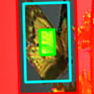
(a)

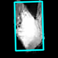
(b)

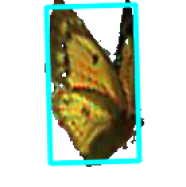
(c)

Figure 3: The alpha matting pipeline. (a) The original, expanded ($\rho^{+}=1.7$), and contracted ($\rho^{-}=0.9$) BBs. The calculated alpha matte (b) and the mask (c) corresponding to a threshold of $\tau=0.80$.

Shrinking the area of the BB and using this region as a scribble mask to represent the object relies on the assumption that the object is located at the centre of the BB, which may not always be the case. If an object is highly non-compact or has holes in it, then there is a possibility of background pixels being included in the scribble mask. Expanding the BB to represent the background also makes the assumption that pixels sufficiently far away from the BB do not belong to the object. This is a stronger assumption, although there may still be cases where parts of an object protruding far from the BB are labelled as background.

The output of the alpha matting process, the alpha matte $\boldsymbol{\mathbf{\alpha}}^{*}$, is not a strict segmentation, but rather a pixel mask indicating what fraction of each pixel is foreground (belonging to the object) and background. A segmentation is produced by thresholding the alpha values to create an object mask. Pixels with a predicted $\alpha_{i}^{*}$ value greater than a threshold $t$ are assigned as belonging to the object, with those whose $\alpha_{i}\leq t$ being labelled as background. The threshold $t$ is chosen so that a proportion $\tau$ of the BB is classified as the object. This allows the alpha threshold $t$ to be dynamically chosen based on how much of the BB is expected to be populated with the object in question. For example, in the VOT2016 competition [2] at least 70% of the BB belongs to the object.

III Evaluation Protocol

In order to evaluate the segmentation performance of each algorithm, we used real-world input in the form of the VOT2016 dataset [2]. It is one of the most widely used datasets in the tracking community, comprising 60 videos, with human-annotated ground-truth BBs and pixel-wise segmentations [13]. In order to increase the number of examples, we used the first, middle, and last frames from each video. Within this dataset, the sizes of the BBs varies widely. The minimum and maximum dimensions were $8.5$ and $511$ pixels respectively, with the mean dimension being $92$ pixels. The number of pixels contained within the BBs ranged from $229$ to $214,773$ with the mean being $12,183$.

The segmentation performance was assessed by the Intersection over Union (IoU) measure, also known as the Jaccard index:

$$\phi_{all}=\frac{\left|\mathcal{G}\cap\mathcal{P}\right|}{\left|\mathcal{G}\cup\mathcal{P}\right|},$$ (11)

where $\mathcal{G}$ and $\mathcal{P}$ are the sets of pixels forming the ground-truth and predicted segmentations. It is worth noting that the IoU measure is equivalent to the Dice similarity coefficient (DSC), also known as the $\text{F}_{1}$ measure, in the sense that $\text{DSC}=2\phi_{all}/(1+\phi_{all})$.

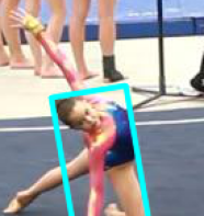
(a)

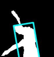
(b)

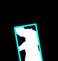
(c)

Figure 4: (a) The original cropped image and BB. Ground truths masks of the (b) full $\phi_{all}$ and (c) BB $\phi_{bb}$ segmentation criterion.

The segmentations were assessed using two criteria, $\phi_{all}$ and $\phi_{bb}$. As illustrated in Fig. 4b, the $\phi_{all}$ measure compares the predicted object mask $\mathcal{P}$ to the ground truth $\mathcal{G}$, including regions of $\mathcal{G}$ that lie outside the BB. This assesses the full segmentation capability of the technique, and allows a tracker to make use of all available information about the object and its background. The $\phi_{bb}$ measure compares the quality of object segmentation and the ground truth within the BB, $\mathcal{B}$; thus

$$\phi_{bb}=\frac{\left|\mathcal{G}\cap\mathcal{P}\cap\mathcal{B}\right|}{\left|(\mathcal{G}\cup\mathcal{P})\cap\mathcal{B}\right|}.$$ (12)

This corresponds to typical use by tracking algorithms which assume that the object lies completely within the BB, and only track the pixels within it.

TABLE I: Parameter values used in cross-validation.

Technique	Parameter	Values
OC-SVM	$\nu$	$0.001,0.002,\ldots,0.005,$ $0.01,0.02,\ldots,0.05,$ $0.1,0.15,\ldots,0.5$
	$\gamma$	$2^{-20},2^{-19},\ldots,2^{20}$
SBBM	$\delta$	$0.1,0.2,\ldots,1.0$
	$\eta$	$0.1,0.2,\ldots,1.0$
LBDM	$\rho^{+}$	$1.1,1.2,\ldots,2.0$
	$\rho^{-}$	$0.1,0.2,\ldots,0.9$
	$\tau$	$0.50,0.51,\ldots,1.00$
	$\lambda$	$10^{0},10^{-1},\ldots,10^{-10}$

Each technique was evaluated using leave-one-out cross-validation based on videos, meaning that the 3 frames from a single video were held out for testing, while the optimal parameters for the technique were determined as those giving the best $\phi_{all}$ or $\phi_{bb}$ score averaged over the 177 frames from the remaining 59 videos. Performance on the 3 held out frames was then evaluated using the cross-validated optimal parameters. This procedure was repeated for each of the other 59 videos held out in turn to obtain average performance metrics.

Each possible combination of the parameter values shown in Table I was evaluated for each technique, with the process being repeated for both $\phi_{all}$ and $\phi_{bb}$. In addition, a baseline performance, denoted as “Entire BB”, was obtained as the segmentation that consists of the entire BB; that is $\mathcal{P}\equiv\mathcal{B}$.

As noted above, the OC-SVM is a feature-based classifier. RGB, LAB, SIFT [19], and LBP [20] features, with the first two being colour-based and the latter two texture-based features, were used for separate experiments within the same testing protocol. RGB histograms are one of many representations of colour data, describing the underlying colour distribution of the image region as seen by physical devices. Unlike RGB, LAB is designed to approximate human vision and is perceptually uniform, i.e. changes in colour values result in the same amount of perceived visual change. We used 8 bins for each channel in both the RGB and LAB feature descriptors to represent each superpixel. SIFT features were the concatenation of SIFT features extracted for each colour channel separately; likewise for LBP. Dense SIFT features were extracted with a $4\times 4$ sliding window and with the orientation set to 0. The feature descriptor extracted nearest to a superpixel’s centroid was assigned as its feature. LBP features from a $5\times 5$ window were extracted, centred on the pixel nearest to the superpixel’s centroid. We used the typical parameters of $P=8$ and $R=2$, with the scale and rotation invariant version of the descriptor, along with the uniform patterns extension [20]. Features were standardised to have zero mean and unit variance before classification.

SBBM uses the raw RGB values of the pixels and a colour radius $R=20$, corresponding to approximately a $4.5\%$ deviation in each colour channel, which we have found to give good results across a range of examples.

TABLE II: Average segmentation performance of each technique for the two overlap measures. The first and second place values are highlighted by red and blue colour respectively.

	Average Performance
Technique	$\phi_{all}$	$\phi_{bb}$
Entire BB	0.579	0.747
OC-SVM + RGB	0.588	0.744
OC-SVM + LAB	0.581	0.745
OC-SVM + SIFT	0.579	0.747
OC-SVM + LBP	0.580	0.748
SBBM	0.555	0.747
Alpha Matting	0.763	0.804

In the alpha matting technique, the neighbourhood $\mathcal{N}_{i}$ was defined to be a $3\times 3$ region centred on the pixel in question, meaning that the size of each pixel’s neighbourhood was $m=8$. We used the RGB values to be the features $\boldsymbol{\mathbf{x}}_{i}$ of each pixel, normalising them such that $[0,255]\mapsto[0,1]$. The alpha matting parameter was set to $c=800$ as this is a large enough penalty, compared with normalised values of $\boldsymbol{\mathbf{x}}_{i}$, to act effectively as $\infty$ [22].

IV Results

Table II gives summary segmentation performance results for both $\phi_{all}$ and $\phi_{bb}$, with Fig. 5 displaying the distribution of scores across the VOT2016 data. The performance of simply predicting the entire BB to be the object, labelled as Entire BB in the figures, acts as a baseline and we note that on average the OC-SVM and SBBM methods perform similarly to the baseline. The range of scores is large for all methods (Fig. 5), indicating that although each method performs well on some images, there others on which it performs poorly.

OC-SVM

We compared segmentations using the cross-validated optimal parameters, with those using the parameters that gave the best result for $\phi_{all}$. A typical example of this can be seen in Fig. 6. In general, we found that the OC-SVM was capable of giving good segmentations, as can be seen in Fig. 6c, but the parameters required to achieve these were widely spread, with no one region of parameter space giving good results for the majority of images.

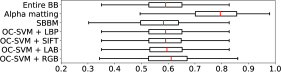
(a)

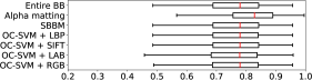
(b)

Figure 5: Distribution of (a) $\phi_{all}$ and (b) $\phi_{bb}$ for each technique.

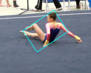
(a)

(b)

(c)

Figure 6: OC-SVM: (a) Original image. (b) Cross validated segmentation ($\gamma=10^{6}$, $\nu=0.004$). (c) Best possible segmentation using LAB features ($\gamma=10^{-19}$, $\nu=0.250$).

It is interesting to note that there is little difference between the performance of the OC-SVM between the colour and texture-based features. In addition to the four feature-descriptors reported, we also combined them by concatenating the feature vectors together. No statistical improvement was found using any combination of features, and all suffered from the same problem as the four main features: good segmentations were too parameter-specific. Likewise, solely grey-scale features did not yield any improvement.

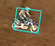
(a)

(b)

(c)

Figure 7: SBBM: (a) Original image. (b) Cross validated segmentation ($\delta=0.1$, $\nu=1.0$). (c) Best possible segmentation ($\delta=0.3$, $\nu=0.1$).

SBBM

Similarly to the OC-SVM, SBBM also demonstrated the same problem of being too parameter dependent. We performed the same comparison of the cross-validated segmentations to the best possible segmentations, an example of which can be seen in Fig. 7. The technique was capable of creating good segmentations on some of the test images, e.g. Fig. 7c, but had a greater range of variation as to how successful the best possible segmentations were, similar to its interquartile range in Fig. 5a.

(a)

(b)

(c)

Figure 8: Alpha matting: (a) Original image. (b) Cross validated ($\rho^{-}=0.8,\rho^{+}=1.2,\tau=0.85,\lambda=10^{-2}$) and (c) best possible segmentations ($\rho^{-}=0.6,\rho^{+}=1.1,\tau=0.85,\lambda=10^{-2}$), with labelled original, expanded, and contracted BBs.

LBDM

The alpha matting technique achieved a much higher segmentation accuracy for both $\phi_{all}$ and $\phi_{bb}$, as can be seen clearly in Fig. 5, and improved on predicting the entire BB as the object by a considerable margin. It tended to perform very well in cases where the contracted BBs, green in Fig. 8, contained solely the object. However, when this region contained background pixels, as is the case in Fig. 9b, these may be labelled as belonging to the object and propagated outwards. As Fig. 9c shows, shrinking and translating the inner BB to include only the object improves the performance, but clearly this is not feasible in practice.

The group of objects whose centre of mass was positioned in some other location than the centre of the BB comprised almost completely of people. As people do not typically stand with their legs close together, and almost never do when in motion, we looked at the cross-validated performance of videos that contain humans (27) and those that do not (33). The average object segmentation performance $\phi_{all}$ for humans and non-humans was 0.718 and 0.800 respectively. Comparing this to the average performance across all videos (0.763) shows that segmenting humans is a harder than average task. This is in contrast to segmenting non-human objects, appearing to be a simpler task, as these typically are more compact. If one is able to detect the object to be tracked is human-like, using a combination of shrinking the inner BB further and translating it upwards, along with using a lower threshold $\tau$ for the amount of object likely in the BB, should improve performance somewhat.

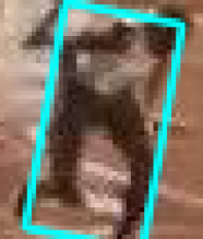
(a)

(b)

(c)

Figure 9: Alpha matting: (a) Original image. (b) Cross validated parameters ($\rho^{-}=0.8$, $\rho^{+}=1.2$, $\tau=0.84$, and $\lambda=10^{-2}$) and (c) changing parameters to $\rho^{-}=0.9$ and $\tau=0.6$, and translating the inner BB up by 9 pixels.

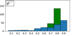
(a)

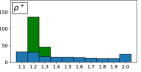
(b)

(c)

(d)

Figure 10: Distribution of the optimal and cross-validated alpha matting parameters for the $\phi_{all}$ measure. (a) $\rho^{-}$, (b) $\rho^{+}$, (c) $\tau$, and (d) $\log_{10}(\lambda)$.

Fig. 10 shows histograms of the parameters which gave the highest performance for each tested frame. The extent to which the BB is shrunk to define scribble mask is controlled by $\rho^{-}$. As Fig. 10a shows, for the majority of images a large shrinkage (small scribble mask) is optimal. This helps to avoid portions of the background, particularly for humans and other non-compact objects. Fig. 10b shows a wide variation in the optimal BB expansion parameter $\rho^{+}$, indicating that in some circumstances it is helpful to include a large part of the adjoining regions, particularly for objects that extend outside the BB. However, the cross-validated optimum suggests an expansion of around 20%.

The values (Fig. 10c) of the fraction of the BB that should be filled by the segmentation, $\tau$, relate directly to the specific problem investigated. The benchmark [2] states that there should be no more than 30% of pixels in the BB containing background, which corresponds well to the region of most optimal parameters, 0.75 to 0.90 in Fig. 10c. Fig. 10d, showing the optimal value of the shrinkage term in the ridge regression, indicates a value between the two values recommended by the technique’s authors ($\lambda=10^{-1}$ in [22] and $\lambda=10^{-7}$ in their published code). This may indicate that the parameter is more problem specific than they anticipated, and may be related to the size of the features used or complexity of the image.

The alpha matting experiments were also repeated with the neighbourhood $\mathcal{N}_{i}$ of each pixel defined as a $7\times 7$ window. This resulted in approximately the same performance as using the $3\times 3$ window, with $\phi_{all}=0.760$ and $\phi_{bb}=0.801$. [22] recommended the use of a $7\times 7$ neighbourhood size to give a more stable image matte, although their images, and therefore the number of unlabelled pixels, were much larger than here. The computational expense is dominated by solving (9) for $\boldsymbol{\mathbf{\alpha}}^{*}$. With $7\times 7$ windows ($m=48$) it is approximately forty times more expensive than for $3\times 3$ windows ($m=8$).

V Conclusion

We have investigated three novel methods of determining the object to be tracked within a limited BB. Two of these, OC-SVM and SBBM, depend on characterising the background image’s colour/texture so that the foreground object can be identified as different. Although both of these methods perform well with tuned parameters, neither is robust enough to allow good performance on novel videos.

An alpha matting method (LBDM), which seeks to extend the foreground object from a presumed scribble mask, gives good performance over the VOT2016 dataset using parameters chosen by cross-validation. It is able to improve upon the assumption of most trackers that the entire BB belongs to the object, and should increase the initial performance of most tracking techniques. The LBDM method relies on the assumption that the centre of the BB is the object to be tracked and its performance is degraded for non-compact objects for which this is not the case.

All of these methods suffer from the paucity of data and we expect improved performance as higher resolution video becomes available. We note that the initialisation problem is significant not only at the start of tracking, but also when re-initialisation is required during tracking.

Source code for all three methods is publicly available at: http://github.com/georgedeath/initialisation-problem.

References

- [1] Y. Wu, J. Lim, and M.-H. Yang, “Online object tracking: A benchmark.” in CVPR, 2013, pp. 2411–2418.
- [2] M. Kristan, A. Leonardis, J. Matas, M. Felsberg, R. Pflugfelder, and L. Čehovin, “The visual object tracking VOT2016 challenge results,” in ECCV, 2016, pp. 777–823.
- [3] J. F. Henriques, R. Caseiro, P. Martins, and J. Batista, “High-speed tracking with kernelized correlation filters,” TPAMI, vol. 37, no. 3, pp. 583–596, 2015.
- [4] H. Nam and B. Han, “Learning multi-domain convolutional neural networks for visual tracking,” in CVPR, 2016, pp. 4293–4302.
- [5] S. Hare, S. Golodetz, A. Saffari, V. Vineet, M. M. Cheng, S. L. Hicks, and P. H. S. Torr, “Struck: Structured output tracking with kernels,” TPAMI, vol. 38, no. 10, pp. 2096–2109, 2016.
- [6] J. Kwon and K. M. Lee, “Tracking of a non-rigid object via patch-based dynamic appearance modeling and adaptive basin hopping monte carlo sampling,” in CVPR, 2009, pp. 1208–1215.
- [7] L. Čehovin, M. Kristan, and A. Leonardis, “Robust visual tracking using an adaptive coupled-layer visual model,” TPAMI, vol. 35, no. 4, pp. 941–953, 2013.
- [8] O. Akin, E. Erdem, A. Erdem, and K. Mikolajczyk, “Deformable part-based tracking by coupled global and local correlation filters,” Journal of Vis. Commun. and Image Representation, vol. 38, pp. 763–774, 2016.
- [9] K. M. Yi, H. Jeong, S. W. Kim, S. Yin, S. Oh, and J. Y. Choi, “Visual tracking of non-rigid objects with partial occlusion through elastic structure of local patches and hierarchical diffusion,” Image and Vis. Comput., vol. 39, pp. 23–37, 2015.
- [10] D. Du, H. Qi, L. Wen, Q. Tian, Q. Huang, and S. Lyu, “Geometric hypergraph learning for visual tracking,” IEEE Trans. Cybern., vol. PP, no. 99, pp. 1–14, 2017.
- [11] J. Xiao, R. Stolkin, and A. Leonardis, “Single target tracking using adaptive clustered decision trees and dynamic multi-level appearance models,” in CVPR, 2015, pp. 4978–4987.
- [12] L. Čehovin, A. Leonardis, and M. Kristan, “Robust visual tracking using template anchors,” in IEEE Winter Conf. on Appl. of Comput. Vis. (WACV), 2016, pp. 1–8.
- [13] T. Vojíř and J. Matas, “Pixel-wise object segmentations for the VOT 2016 dataset,” Center for Machine Perception, Czech Technical University, Prague, Czech Republic, Research Report CTU-CMP-2017-01, 2017.
- [14] B. Schölkopf, J. C. Platt, J. C. Shawe-Taylor, A. J. Smola, and R. C. Williamson, “Estimating the support of a high-dimensional distribution,” Neural Comput., vol. 13, no. 7, pp. 1443–1471, 2001.
- [15] C.-C. Chang and C.-J. Lin, “LIBSVM: A library for support vector machines,” ACM Trans. on Intell. Syst. and Technol., vol. 2, pp. 1–27, 2011.
- [16] B. Schölkopf and A. J. Smola, Learning with Kernels. Cambridge, MA, USA: MIT Press, 2001.
- [17] D. M. Tax and R. P. Duin, “Support vector data description,” Machine Learning, vol. 54, no. 1, pp. 45–66, 2004.
- [18] R. Achanta, A. Shaji, K. Smith, A. Lucchi, P. Fua, and S. Süsstrunk, “SLIC superpixels compared to state-of-the-art superpixel methods,” TPAMI, vol. 34, no. 11, pp. 2274–2282, 2012.
- [19] D. G. Lowe, “Object recognition from local scale-invariant features,” in ICCV, vol. 2, 1999, pp. 1150–1157.
- [20] T. Ojala, M. Pietikäinen, and T. Mäenpää, “Multiresolution gray-scale and rotation invariant texture classification with local binary patterns,” TPAMI, vol. 24, no. 7, pp. 971–987, 2002.
- [21] O. Barnich and M. V. Droogenbroeck, “ViBe: A universal background subtraction algorithm for video sequences,” IEEE Trans. Image Process., vol. 20, no. 6, pp. 1709–1724, 2011.
- [22] Y. Zheng and C. Kambhamettu, “Learning based digital matting,” in ICCV, 2009, pp. 889–896.
- [23] Y.-Y. Chuang, B. Curless, D. H. Salesin, and R. Szeliski, “A bayesian approach to digital matting,” in CVPR, vol. 2, 2001, pp. 264–271.