Implicit numerical schemes for generalized heat conduction equations

Abstract

There are various situations where the classical Fourier’s law for heat conduction is not applicable, such as heat conduction in heterogeneous materials [1, 2] or for modeling low-temperature phenomena [3, 4, 5]. In such cases, heat flux is not directly proportional to temperature gradient, hence, the role – and both the analytical and numerical treatment – of boundary conditions becomes nontrivial. Here, we address this question for finite difference numerics via a shifted field approach. Based on this ground, implicit schemes are presented and compared to each other for the Guyer–Krumhansl generalized heat conduction equation, which successfully describes numerous beyond-Fourier experimental findings. The results are validated by an analytical solution, and are contrasted to finite element method outcomes obtained by COMSOL.

1 Introduction

The need to go beyond the Fourier heat conduction equation – which reads in one spatial dimension

$$\partial_{t}T=\alpha\partial_{xx}T$$ (1)

for temperature $T$, with thermal diffusivity $\alpha$, and which contains only first order time derivative $\partial_{t}$ and second order space derivative $\partial_{xx}$ – is experimentally proved under various conditions since decades [1, 2, 6, 7, 8, 9, 10, 11]. These circumstances are related partly to the material structure [12, 13], and partly to the environment like temperature and excitation [33]. The characteristics of the interaction between the sample and the environment are condensed into the boundary conditions, the role of which are therefore crucial during the modeling.

For theories beyond the Fourier one, the common starting point is the balance equation of internal energy $e$,

$$\rho\partial_{t}e+\partial_{x}q=0,$$ (2)

also written in one spatial dimension, with density $\rho$ and heat flux $q$. For many applications, a constant specific heat $c$ can be assumed, yielding $e=cT$.

Then, if one takes Fourier’s law,

$$q=-k\partial_{x}T,$$ (3)

where $k$ is thermal conductivity, then (1) can be obtained. In parallel, heat flux boundary conditions – like a heat pulse on one end and an adiabatic insulation on the other one, the case considered hereafter – can be written directly for temperature, prescribing its gradient.

However, for generalized heat conduction models, the picture is not so simple any more. For example, in the first known extension to Fourier’s law, the so-called Maxwell–Cattaneo–Vernotte (MCV) constitutive equation [14, 15, 16, 17]

$$\tau_{q}\partial_{t}q+q=-k\partial_{x}T,$$ (4)

time derivative of heat flux also appears, accompanied by a coefficient $\tau_{q}$ called relaxation time. In this case a heat flux boundary condition cannot be translated to a Neumann-type boundary condition on temperature. The situation becomes even more involved for the Guyer–Krumhansl (GK) equation [18, 19, 20],

$$\tau_{q}\partial_{t}q+q=-k\partial_{x}T+\kappa^{2}\partial_{xx}q,$$ (5)

where $\kappa^{2}$ is a parameter strongly related to the mean free path from the aspect of kinetic theory [21]. According to room-temperature experiments [1, 2, 33], measured deviation from the Fourier prediction always occurs in the overdamped ($\kappa^{2}>\tau_{q}$) region (as opposed to the near-to-MCV region $\kappa^{2}<\tau_{q}$), thus usage of the GK equation is inescapable.

Combining (5) with (2) provides the temperature-only version of the GK model:

$$\tau_{q}\partial_{tt}T+\partial_{t}T=\alpha\partial_{xx}T+\kappa^{2}\partial_{txx}T.$$ (6)

Solving this equation with heat flux boundary conditions, especially with time dependent ones needed for evaluating heat pulse experiments [1, 2], is difficult. It is not clear how to translate conditions on $q(t)$ to temperature $T(t)$, the two quantities being related to one another according to a constitutive equation (5). This was the motivation to develop a simple and fast numerical scheme, a scheme of shifted fields [3], that was specifically devised to be suitable for this type of problem. The term shifted fields refers here to the spatial discretization method. Namely, instead of solving (6) for $T$, the set of equations (2) and (5) are solved for $T$ and $q$ both, where spatial locations of temperature values are shifted by a half space step with respect to locations of $q$ values (see Fig. 1). This enables us to prescribe boundary conditions only for heat flux.

Figure 1: Discretization method of shifted fields for a heat pulse setting. Prescribed boundary values are $q_{1}$ as a function of time, and $q_{J}=0$ representing adiabatic insulation. All other values (illustrated by filled rectangles and circles) can be computed from neighboring and previous values. Temperature values sit at cell midpoints while heat flux values reside at cell boundaries.

A physical interpretation of such a scheme is the distinction between surface-related and volume-related quantities of the discrete cells. More closely, temperature represents the average value over the volume while heat flux describes energy flow at the cell boundary.

Notably, similar but different schemes like the two-step Lax-Wendroff, leapfrog or Finite-Difference-Time-Domain (FDTD) methods are known in the literature. All these apply values at half time step or half space step to update a grid point at the next time instant [22]. Furthermore, the present shifted field concept also differs from the multigrid method where the goal is to increase accuracy by applying finer and finer meshes [22, 23]. One should also mention Feynman [24] who presents a technique for time integration for the dynamics of a point particle where the shifting is used for time steps only. Moreover, Yee discusses the problem of electromagnetic wave propagation and applies the FDTD method to solve the Maxwell equations, and also discusses the possible boundary conditions for such wave propagation problem [25]. However, none of the mentioned techniques address the question of boundary conditions, and the advantage of the shifted strategy for boundary conditions – especially such nontrivial ones – is not realized. One should also pay attention to the work of Berezovski et al. [26, 27, 28, 29, 30] where remarkably efficient numerical schemes are developed and tested for wave propagation problems.

Our approach uses simple finite differences to approximate the partial derivatives. An explicit version has already been developed [3]; here we present the realization of the corresponding implicit version, which turns out to be remarkably superior in performance aspects. The outcomes are also compared to analytical and finite element solutions in respect of efficiency and speed.

2 Explicit scheme

For the explicit scheme, all related analysis and detailed discussion are published in [3], and are only summarized here for the sake of completeness. Hereafter, dimensionless quantities [3] are used, which is a framework that is simple yet satisfactory for the current numerics-related considerations.

The discretized form of the balance equation of internal energy (2) is

$$T^{n+1}_{j}=T^{n}_{j}-\frac{\Delta t}{\tau_{\Delta}\Delta x}(q^{n}_{j+1}-q^{n}_{j}),$$ (7)

where $n$ indexes time steps and $j$ the space steps, $\tau_{\Delta}$ denotes the dimensionless pulse duration time and $\Delta t$ the time step. The Guyer–Krumhansl constitutive equation is discretized as

$$q^{n+1}_{j}=q^{n}_{j}-\frac{\Delta t}{\tau_{q}}q^{n}_{j}-\frac{\tau_{\Delta}\Delta t}{\tau_{q}\Delta x}(T^{n}_{j}-T^{n}_{j-1})+\frac{\kappa^{2}\Delta t}{\tau_{q}\Delta x^{2}}(q^{n}_{j+1}-2q^{n}_{j}+q^{n}_{j-1}),$$ (8)

which is able to reproduce the solutions of the MCV model ($\kappa=0$) and of the Fourier one ($\tau_{q}=\kappa^{2}$). In these formulae, forward time differencing is applied, which makes all the schemes first order in time. Let us draw attention again to the boundary conditions, thanks to which $T$ values can be updated without prescribing anything for temperature at the boundaries.

The scheme being explicit, one has to calculate the stability criteria as well. In [3], von Neumann and Jury methods [22, 31] are used to determine the stability conditions. In order to prove the convergence of such a scheme, the Lax–Richtmyer theorem [32] is exploited by proving the consistency of the schemes together with their stability. Regarding consistency, although only its weak form is proved [33], it is enough to fulfill the Lax–Richtmyer theorem and ensure the presence of convergence [34, 35].

3 Implicit schemes

When quantities at time instant $t^{n+1}$ are also considered, the scheme becomes implicit, leading to the following discretized form of the balance equation of internal energy:

$$\tau_{\Delta}\frac{1}{\Delta t}(T^{n+1}_{j}-T^{n}_{j})=-\frac{1}{\Delta x}\left[(1-\Theta)\left(q^{n}_{j+1}-q^{n}_{j}\right)+\Theta\left(q^{n+1}_{j+1}-q^{n+1}_{j}\right)\right],$$ (9)

and of the GK-type constitutive equation:

$$\frac{\tau_{q}}{\Delta t}\left(q^{n+1}_{j}-q^{n}_{j}\right)+\left[(1-\Theta)q^{n}_{j}+\Theta q^{n+1}_{j}\right]$$

$$+\frac{\tau_{\Delta}}{\Delta x}\left[(1-\Theta)(T^{n}_{j}-T^{n}_{j-1})+\Theta(T^{n+1}_{j}-T^{n+1}_{j-1})\right]$$ (10)

$$-\frac{\kappa^{2}}{\Delta x^{2}}\left[(1-\Theta)\big{(}q^{n}_{j+1}-2q^{n}_{j}+q^{n}_{j-1}\big{)}+\Theta\big{(}q^{n+1}_{j+1}-2q^{n+1}_{j}+q^{n+1}_{j-1}\big{)}\right] =0,$$

where the convex combination of explicit and implicit terms is characterized by the parameter $\Theta$, with $\Theta=0$ removing the implicit terms and returning the purely explicit scheme. Analogously, for $\Theta=1$, all the explicit terms vanish, making (9) and (3) purely implicit. Choosing $\Theta=1/2$ gives the so-called Crank–Nicolson scheme, which preserves the unconditionally stable property of implicit schemes and provides one order higher accuracy. Here, accuracy is not analyzed in detail. We test the implicit scheme with settings $\Theta=1/2$ and $\Theta=1$, for various parameter values for $\tau_{q}$ and $\kappa^{2}$.

In order to prove that no stability condition is needed for these implicit schemes, we use the methods of von Neumann and Jury as before [3], i.e., let us assume the solution of the difference equations (9) and (3) in the form

$$\phi^{n}_{j}=\xi^{n}e^{ikj\Delta x},$$ (11)

where $i$ is the imaginary unit, $k$ is the wave number parameter of the solution, $j\Delta x$ denotes the $j^{\text{th}}$ discrete spatial position, and the complex number $\xi$ is called the growth factor [22]. The scheme is stable if and only if $|\xi|\leq 1$ holds. Now, using (11) one can express each term from (9)–(3), for example $q^{n+1}_{j+1}=\xi^{n+1}e^{ik(j+1)\Delta x}\cdot q_{0}$. Substituting back (11) into (9) and (3) yields

$$T_{0}(\xi-1)+q_{0}\frac{\Delta t}{\tau_{\Delta}\Delta x}\left[(1-\Theta)\big{(}e^{ik\Delta x}-1\big{)}+\Theta\xi\big{(}e^{ik\Delta x}-1\big{)}\right] =0,$$ (12)

$$q_{0}(\xi-1)+q_{0}\frac{\Delta t}{\tau_{q}}\left[(1-\Theta)+\Theta\xi\right]$$

$$+T_{0}\frac{\tau_{\Delta}\Delta t}{\Delta x\tau_{q}}\left[(1-\Theta)\big{(}1-e^{-ik\Delta x}\big{)}+\Theta\xi\big{(}1-e^{-ik\Delta x}\big{)}\right]$$

$$-q_{0}\frac{\kappa^{2}\Delta t}{\Delta x^{2}\tau_{q}}\left[(1-\Theta)\left(e^{ik\Delta x}-2+e^{-ik\Delta x}\right)+\Theta\xi\left(e^{ik\Delta x}-2+e^{-ik\Delta x}\right)\right] =0.$$ (13)

Then constructing a coefficient matrix and calculating its determinant leads to the characteristic polynomial of system (12) in the form $F(\xi)=a_{2}\xi^{2}+a_{1}\xi+a_{0}$ with the coefficients: coefficients

$$a_{0} =1-\frac{\Delta t}{\tau_{q}}(1-\Theta)+\left[2\cos(k\Delta x)-2\right]\left(1-\Theta\right)\frac{\Delta t}{\Delta x^{2}\tau_{q}}\left[\kappa^{2}-\Delta t(1-\Theta)\right],$$

$$a_{1} =-2+\frac{\Delta t}{\tau_{q}}(1-2\Theta)+\left[2\cos(k\Delta x)-2\right]\frac{\Delta t}{\Delta x^{2}\tau_{q}}\left[\kappa^{2}(2\Theta-1)-2\Delta t\left(1-\Theta\right)\Theta\right],$$

$$a_{2} =1+\frac{\Delta t}{\tau_{q}}\Theta-\left[2\cos(k\Delta x)-2\right]\frac{\Delta t}{\Delta x^{2}\tau_{q}}\Theta\big{(}\kappa^{2}+\Delta t\Theta\big{)}.$$ (14)

The Jury criteria [31] can be used to obtain the requirements in order to ensure that the roots of characteristic polynomial remain within the unit circle in the complex plane. These criteria are, for the polynomial $F$:

1. $F(\xi=1)>0$,

2. $F(\xi=-1)>0$,

3. $|a_{0}|<a_{2}$.

Calculating each condition for $\Theta=1$ gives us

1. $\frac{4\Delta t^{2}}{\tau_{q}\Delta x^{2}}>0$,

2. $4+2\frac{\Delta t}{\tau_{q}}+4\frac{\Delta t}{\tau_{q}\Delta x^{2}}(2\kappa^{2}+\Delta t)>0$,

3. $1<1+\frac{\Delta t}{\tau_{q}}+4\frac{\Delta t}{\tau_{q}\Delta x^{2}}(\kappa^{2}+\Delta t)$,

hence, the scheme has met the requirements as long as all parameters are positive. In case of $\Theta=1/2$, we have

1. $\frac{4\Delta t^{2}}{\tau_{q}\Delta x^{2}}>0$,

2. $4>0$,

3. $0<1+\frac{4\kappa^{2}}{\Delta x^{2}}$,

that is, the first Jury criterion gives the same result and the other two conditions are simpler and naturally fulfilled again. We remark that, for the MCV equation ($\kappa=0$), each criteria are fulfilled, too. Therefore, the schemes are stable and convergent.

4 Comparison with analytical solutions

Analytical solution for the GK equation is known for several cases [36, 37, 38, 39], even for boundary conditions related to heat pulse experiments with adiabatic condition on the rear side [40]. The analytical solution is available in an infinite sum form [40]. For the benchmark comparison between analytical and numerical solutions presented here, the following parameters have been applied:

1. Solution of Fourier equation: $\tau_{q}=\kappa^{2}$,

2. Solution of MCV equation: $\tau_{q}=0.02$, $\kappa^{2}=0$,

3. Over-diffusive solution of the GK equation: $\tau_{q}=0.02$, $\kappa^{2}=10\tau_{q}$.

Moreover, heat pulse duration $\tau_{\Delta}=0.04$ is used in all cases, and the simulated time interval (dimensionless time $t=1$) and the number of cells ($300$) are also fixed. The various schemes are compared based on the computational run time measured by MATLAB. Although the run time itself is not representative in a single scheme and depends on many other conditions like programming language, realization of a scheme, properties of hardware, etc., for comparative reasons it is useful and representative. It is important to emphasize that the over-diffusive range ($\kappa^{2}>\tau_{q}$) is distinguished by experiments, i.e., the measured non-Fourier behavior always occurs in that region of parameters.

1. Case of the Fourier equation:

   1. $\Theta=1$ scheme requires $100$ time steps and the solution takes $0.119$ s (see Fig. 2).

   2. $\Theta=1/2$ scheme shows no difference either in accuracy or in run time.

   3. $\Theta=0$ explicit scheme requires ca. $10^{6}$ time steps, which takes $142.9$ s.

   4. The analytical solution requires $50$ terms and takes $0.08$ s with $100$ time steps (see Fig. 2).

2. Case of the MCV equation:

   1. For $\Theta=1$ scheme, $1000$ time steps are not sufficient. The solution was not accurate enough (see Fig. 3). With a new setting of $10^{5}$ time steps, solution takes $15.4$ s (Fig. 4).

   2. $\Theta=1/2$ scheme shows significant difference especially for hyperbolic equations like the MCV one. The vicinity of the wave front is more accurate than in the previous case, $1000$ time steps are sufficient and it requires $0.2$ s.

   3. $\Theta=0$ explicit scheme requires ca. $10^{6}$ time steps again, which takes $145.5$ s.

   4. The analytical solution requires $200$ terms and takes $6.6$ s with $500$ time steps (see Fig. 5).

3. Case of the GK equation:

   1. $\Theta=1$ scheme requires $100$ time steps and the solution takes $0.261$ s (see Fig. 6).

   2. $\Theta=1/2$ scheme shows no difference either in accuracy or in run time.

   3. $\Theta=0$ explicit scheme requires ca. $10^{7}$ time steps, which takes $1640$ s.

   4. The analytical solution requires $5$ terms and takes $0.07$ s with $200$ time steps (see Fig. 6).

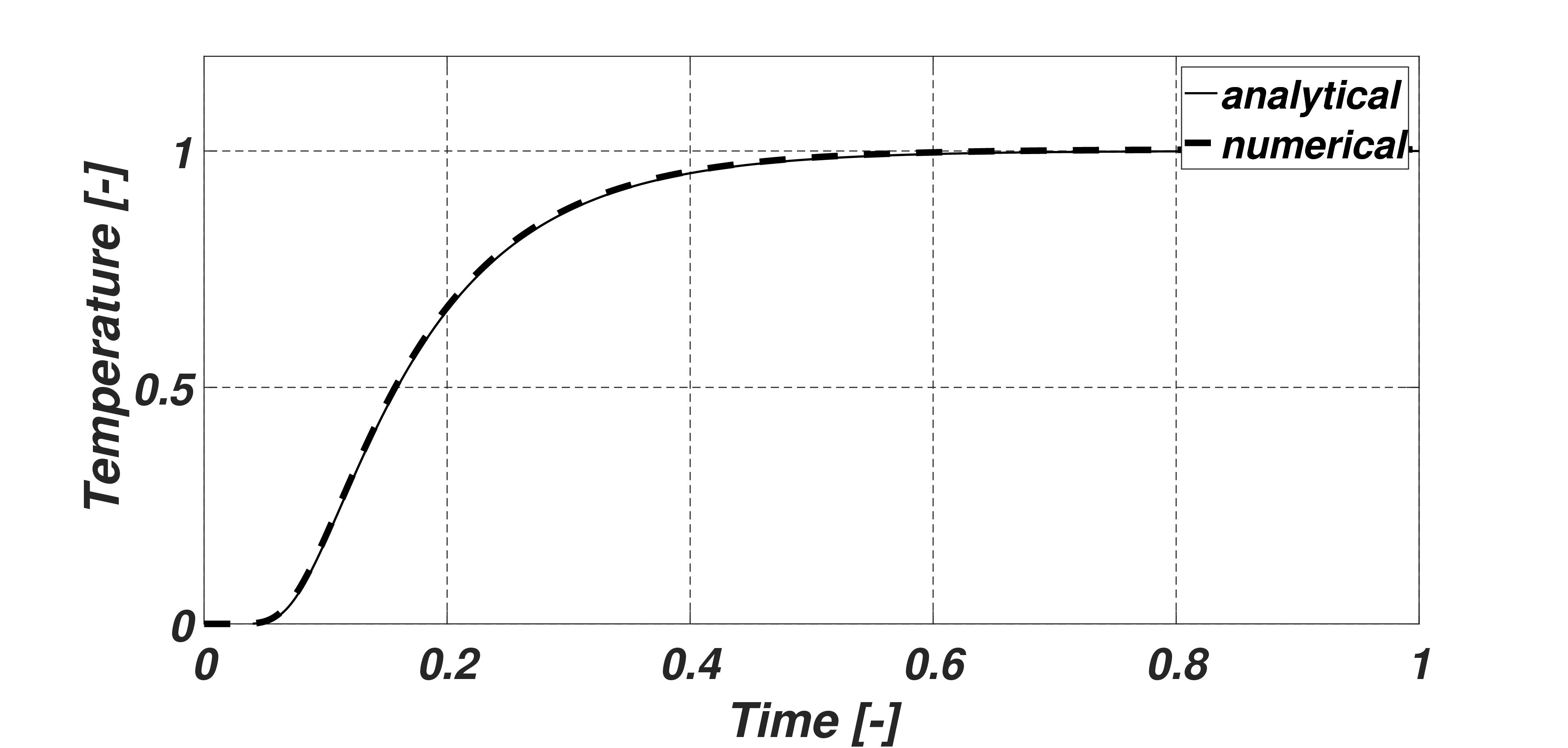
Figure 2: Rear-side temperature histories: the analytical solution (solid line) and the $\Theta=1$ scheme (thicker dashed line).

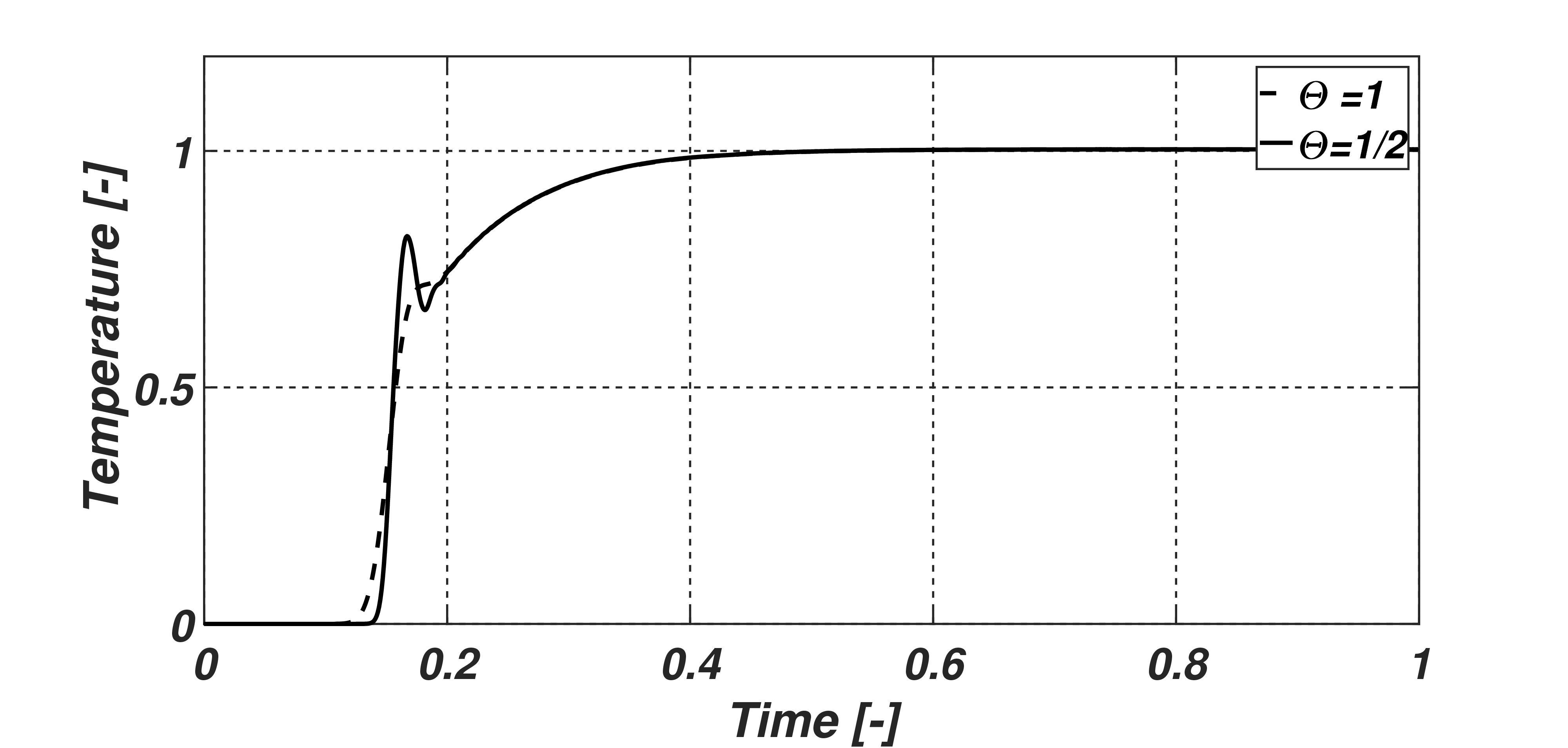
Figure 3: Rear-side temperature histories when solving the MCV equation with schemes $\Theta=1$ ($1000$ time steps) and $\Theta=1/2$. The dashed line belongs to $\Theta=1$.

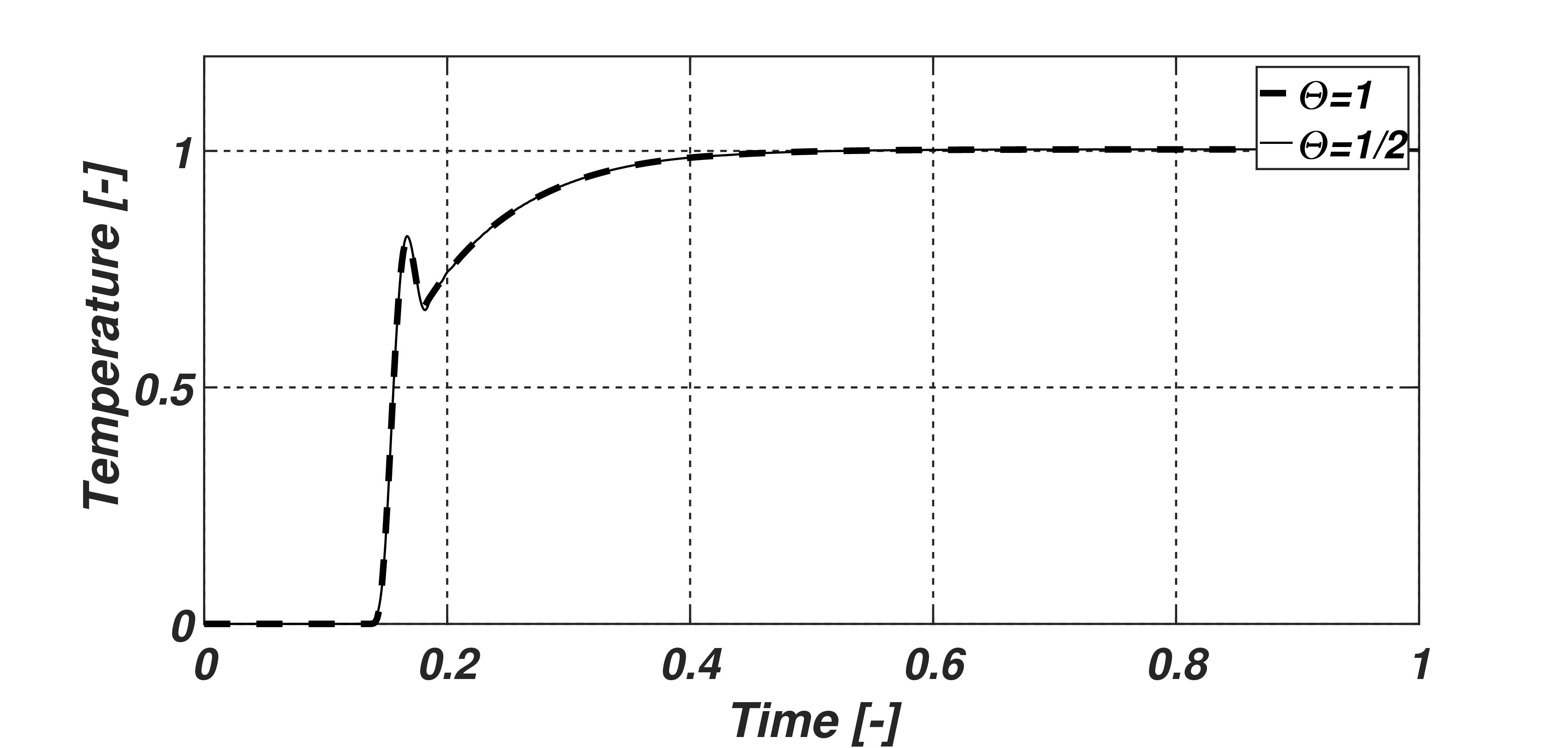
Figure 4: Rear-side temperature histories when solving the MCV equation with schemes $\Theta=1$ ($10^{5}$ time steps) and $\Theta=1/2$. The dashed line belongs to $\Theta=1$.

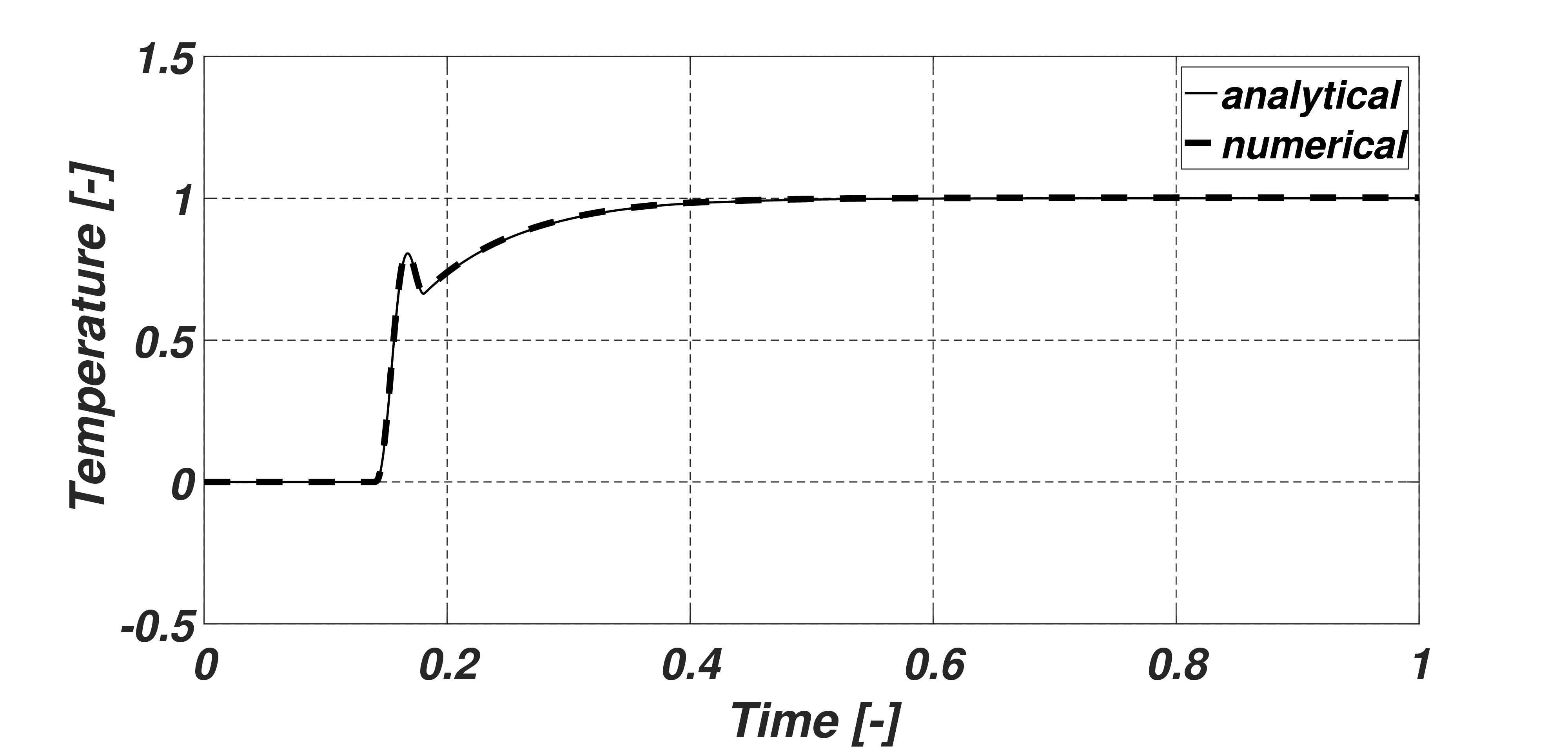
Figure 5: Rear-side temperature histories: comparison between the analytical solution (solid line) and the $\Theta=1/2$ scheme (thicker dashed line).

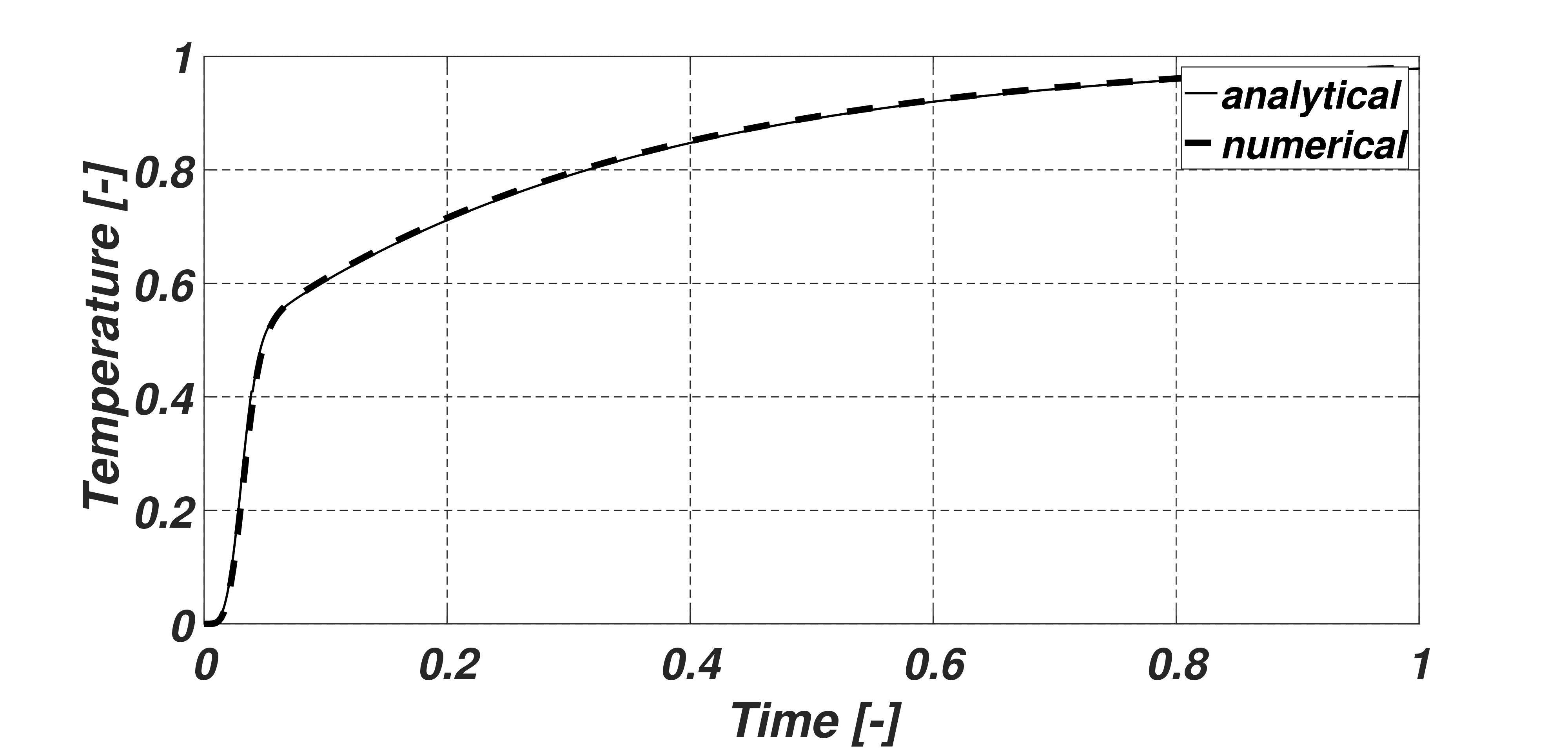
Figure 6: Rear-side temperature histories: comparison between the analytical solution (solid line) and the $\Theta=1$ scheme (thicker dashed line).

As it is clear, the implicit schemes reproduce the analytical solution in every case. In fact, they could be faster for solutions containing jumps like in case of the MCV equation. Moreover, the capabilities of the analytical solution approach are more limited – for example, the GK equation for finite time heat pulse excitation with cooling boundary conditions is not yet solved. In such cases the numerical methods are the only way to obtain the solution. It is important to observe the significant difference between $\Theta=1$ and $1/2$ schemes for hyperbolic equations. The explicit scheme was the slowest and less efficient, not surprisingly.

5 Comparison with finite element method

In this section, the finite element implementation of the same problem is presented, using the software COMSOL v5.3a.

Theoretically, it is possible to implant any kind of partial differential equation within the COMSOL environment. However, to obtain a solution of a generalized heat equation is not as easy as it seems to be. Let us begin with the MCV equation. In order to achieve a smooth solution around the wave front, $100$ elements were used together with the Runge–Kutta (RK34) time stepping method, which requires $600$ time steps. Its run time was $44$ s, and for the solution see Fig. 7. It is to be noted that the simulated time interval was shorter, $0.6$ instead of $1$. The COMSOL solution is hardly faster than the explicit scheme presented above, and is much slower than the Crank–Nicolson-type implicit scheme.

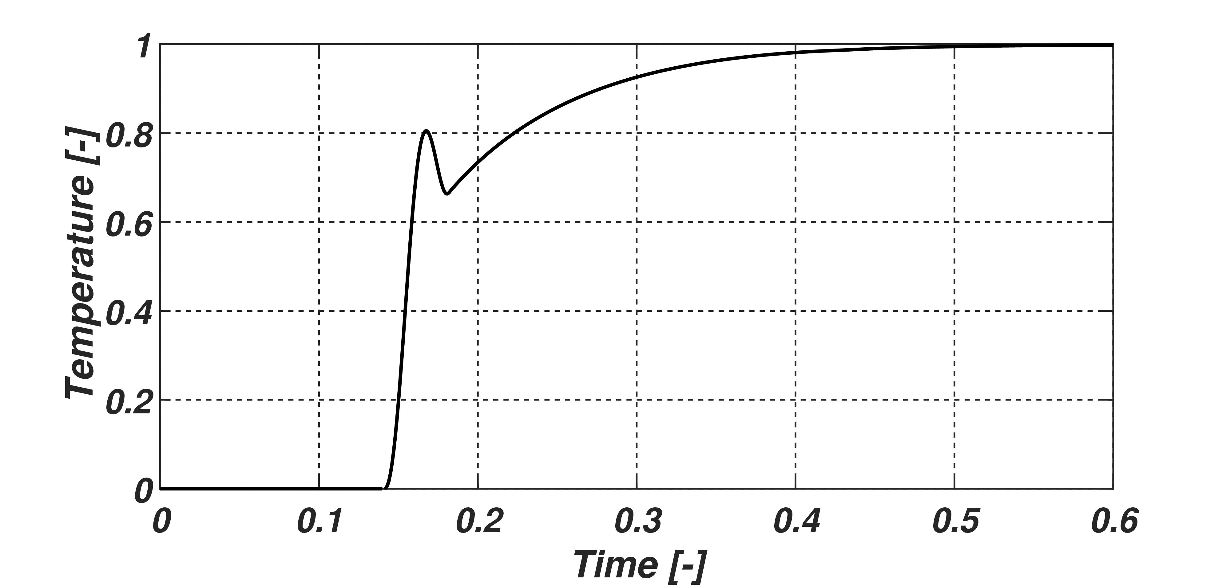
Figure 7: The rear-side temperature history related to the MCV equation ($\tau_{q}=0.02$, $\kappa^{2}=0$), calculated by COMSOL.

When we turn towards the full GK equation, obtaining the solution is not straightforward at all. Although COMSOL reproduces temperature history at the rear side (Fig. 8) in the Fourier-type special case, Fig. 9 presents a false one with $\tau_{q}=0.02$ and $\kappa^{2}=0.2$. Instead of the breakage (like the one in Fig. 6), a false wave-shaped solution appears that does not exist either in the finite difference solution or in the analytical one. Moreover, the appearance of this numerical artifact is independent of mesh and time step sizes, and becomes bigger as $\kappa^{2}$ is increased. Applying again $100$ elements together with a time step of $0.001$, it takes $65$ s to run (Fig. 9). Hence, COMSOL seems not to be applicable to solve the GK equation in the highly over-damped domain.

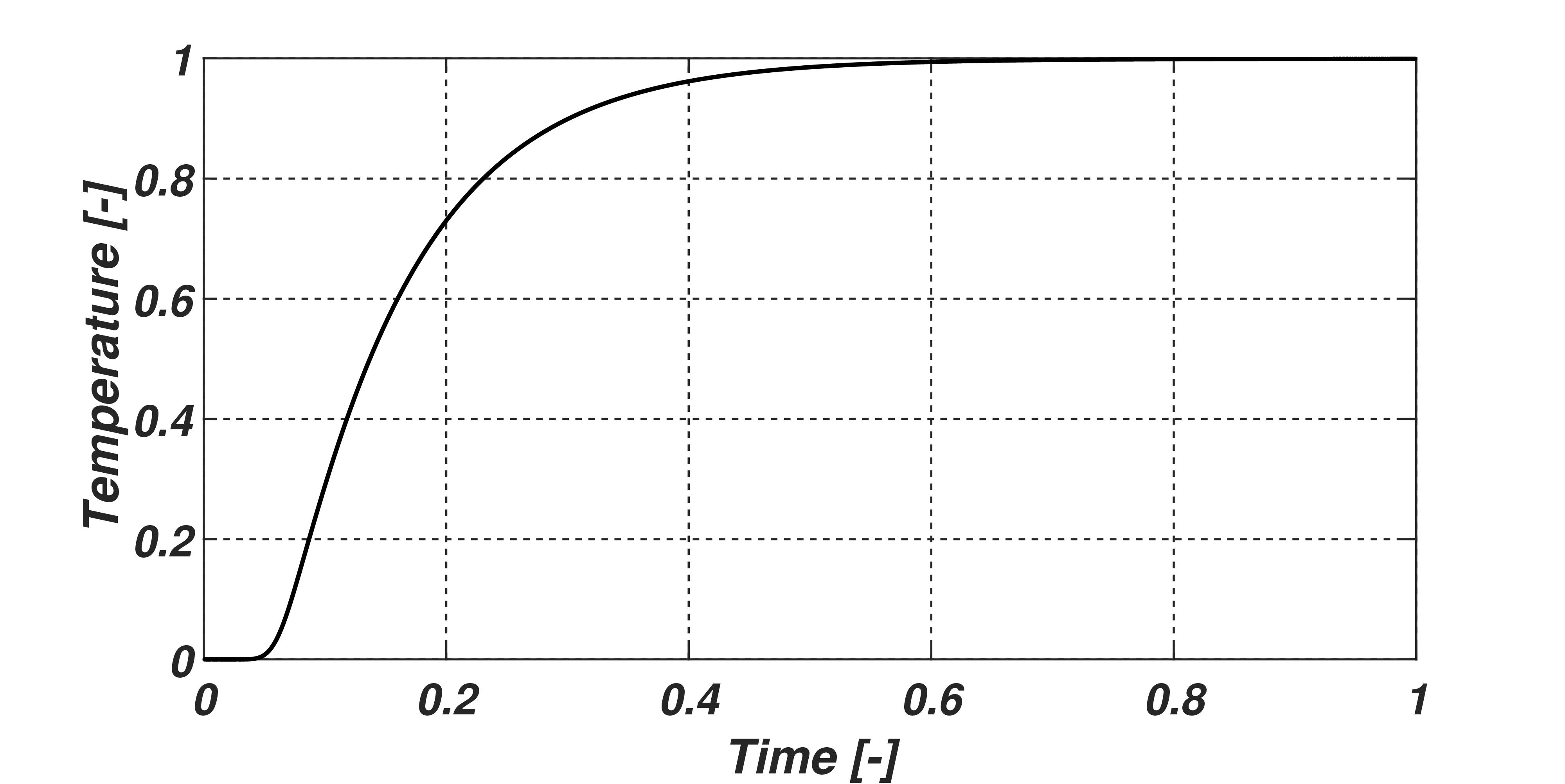
Figure 8: The rear-side temperature history related to the GK equation ($\tau_{q}=\kappa^{2}$), calculated by COMSOL.

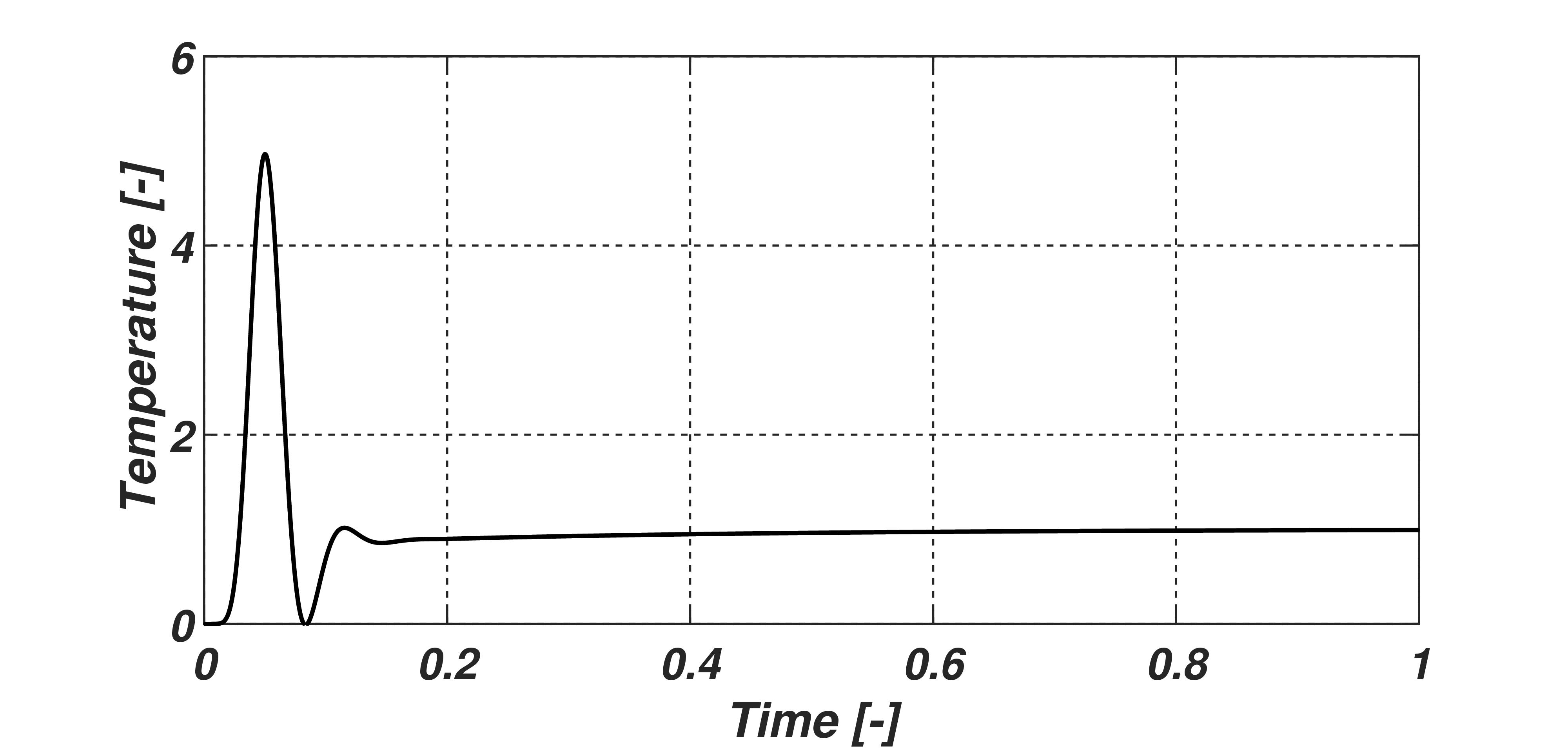
Figure 9: The rear-side temperature history related to the GK equation ($\tau_{q}=0.02$, $\kappa^{2}=0.2$), calculated by COMSOL.

6 Outlook for the ballistic-conductive equation

The ballistic-conductive (BC) equation is a next-level generalization beyond the GK equation, and is strongly related to the low-temperature phenomenon called ballistic heat conduction [3, 41, 42, 43, 44]. Indeed, the BC model has been found to be necessary for explaining low-temperature experiments [4, 5]. Such a hyperbolic equation is more challenging to solve, due to the double characteristic speed and the sharper jumps in certain parameter range. It is possible to derive the implicit schemes for this model as well, as presented below. The system of partial differential equations in question, in dimensionless form, reads

$$\tau_{q}\frac{\partial q}{\partial t}+q+\tau_{\Delta}\frac{\partial T}{\partial x}+\kappa\frac{\partial Q}{\partial x} =0,$$ (15)

$$\tau_{Q}\frac{\partial Q}{\partial t}+Q+\kappa\frac{\partial q}{\partial x} =0,$$

and in the discretized form:

$$\frac{\tau_{q}}{\Delta t}(q^{n+1}_{j}-q^{n}_{j})+\left((1-\Theta)q^{n}_{j}+\Theta q^{n+1}_{j}\right)$$

$$+\frac{\tau_{\Delta}}{\Delta x}\left((1-\Theta)(T^{n}_{j}-T^{n}_{j-1})+\Theta(T^{n+1}_{j}-T^{n+1}_{j-1})\right)$$

$$+\frac{\kappa}{\Delta x}\left((1-\Theta)(Q^{n}_{j}-Q^{n}_{i-1})+\Theta(Q^{n+1}_{j}-Q^{n+1}_{j-1})\right) =0,$$ (16)

$$\frac{\tau_{Q}}{\Delta t}(Q^{n+1}_{j}-Q^{n}_{j})+\left((1-\Theta)Q^{n}_{j}+\Theta Q^{n+1}_{i}\right)$$

$$+\frac{\kappa}{\Delta x}\left[(1-\Theta)(q^{n}_{j+1}-q^{n}_{j})+\Theta(q^{n+1}_{j+1}-q^{n+1}_{j})\right] =0,$$ (17)

where a further variable $Q$ appears as a current density of heat flux [3]. The related relaxation time is denoted by $\tau_{Q}$. The system (16)–(17) can be solved together with the balance equation of internal energy (9). Let us use the parameters $\tau_{\Delta}=0.0076$, $\tau_{q}=0.0186$, $\tau_{Q}=0.007$, $\kappa=0.108$, which are taken from [5] and are related to the evaluation of a ballistic heat conduction phenomenon. The same accuracy properties of implicit schemes are experienced as previously in case of the MCV equation, namely, the one with $\Theta=1/2$ is more accurate in the vicinity of wave front than the one with $\Theta=1$, see Fig. 10 for details. It is sufficient for Crank–Nicolson-type scheme to use $300$ cells with $5000$ time steps which takes $1.8$ s to solve.

In contrast, the COMSOL software is much slower and less accurate, i.e., it produces the same mesh and time step dependent oscillations and jumps, see Fig. 11. Only the last jump corresponds to a real solution, despite of the $1000$ cells used in the simulation with $9000$ time steps. The run time was $186$ s. Should one want to avoid these artificial oscillations, the simulation would require at least ten times more cells and time steps, and it would take hours for COMSOL to solve the BC model with these settings, in contrast with the $1.8$ s run time of the Crank–Nicolson-type approach.

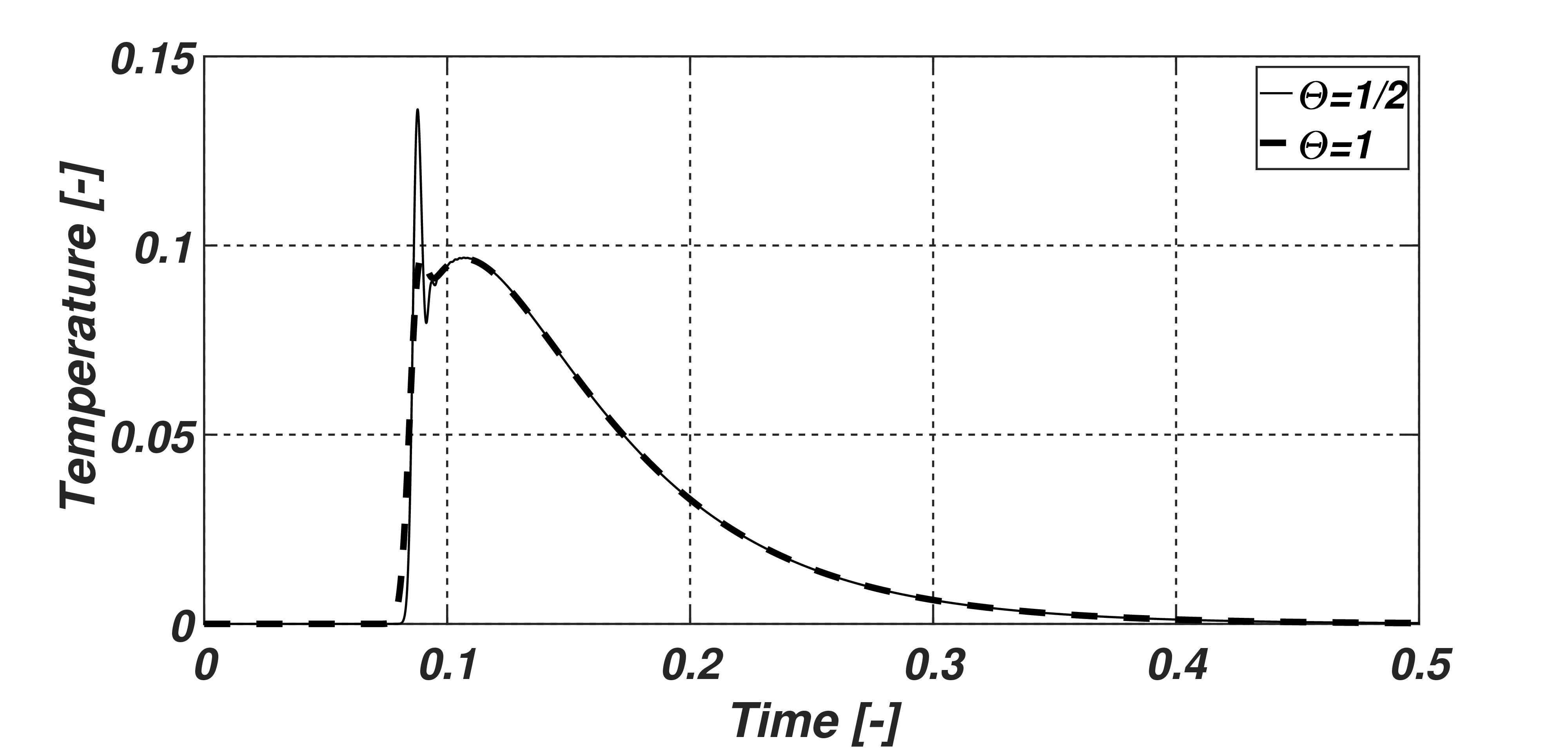
Figure 10: The rear-side temperature histories when solving BC equation with schemes $\Theta=1$ and $\Theta=1/2$. The dashed line belongs to $\Theta=1$.

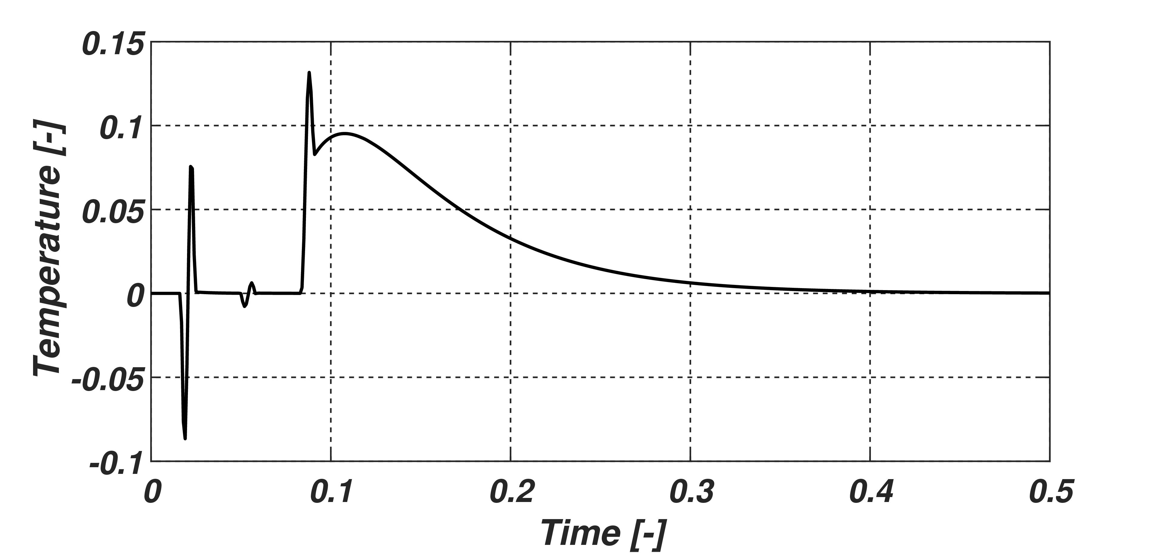
Figure 11: The rear-side temperature history related to BC equation, calculated by COMSOL.

7 Summary

Finite difference numerical schemes based on the shifted field concept have been presented and tested in several cases. It turned out that the Crank–Nicolson-type implicit scheme is the most accurate, especially in solving hyperbolic partial differential equations. Not surprisingly, the presented implicit schemes proved much faster than the explicit one. We also focused on the validation of numerical schemes using the analytical solution of the GK equation. It is important to highlight that the analytical solutions are strongly limited as, for more natural boundary conditions like heat transfer at the boundary is not yet obtained. However, having analytical solution is not absolutely necessary in presence of such a fast and reliable numerical scheme.

The commercial software COMSOL has also been applied for comparison. We have demonstrated that solving generalized heat equations is challenging for finite element methods, and leads in some cases to false solutions so result have to be validated as extensively as possible.

8 Acknowledgements

This work was supported by the National Research, Development and Innovation Office of Hungary (NKFIH) via grants NKFIH K116197, K116375, K124366 and K124508.

References

- [1] S. Both, B. Czél, T. Fülöp, G. Gróf, Á. Gyenis, R. Kovács, P. Ván, J. Verhás, Deviation from the Fourier law in room-temperature heat pulse experiments, Journal of Non-Equilibrium Thermodynamics 41 (1) (2016) 41–48.
- [2] P. Ván, A. Berezovski, T. Fülöp, G. Gróf, R. Kovács, Á. Lovas, J. Verhás, Guyer-Krumhansl-type heat conduction at room temperature, EPL 118 (5) (2017) 50005, arXiv:1704.00341v1.
- [3] R. Kovács, P. Ván, Generalized heat conduction in heat pulse experiments, International Journal of Heat and Mass Transfer 83 (2015) 613 – 620.
- [4] R. Kovács, P. Ván, Models of Ballistic Propagation of Heat at Low Temperatures, International Journal of Thermophysics 37 (9) (2016) 95.
- [5] R. Kovács, P. Ván, Second sound and ballistic heat conduction: NaF experiments revisited, International Journal of Heat and Mass Transfer 117 (2018) 682–690, submitted, arXiv preprint arXiv:1708.09770.
- [6] V. Peshkov, Second sound in Helium II, J. Phys. (Moscow) 381 (8).
- [7] H. E. Jackson, C. T. Walker, T. F. McNelly, Second sound in NaF, Physical Review Letters 25 (1) (1970) 26–28.
- [8] H. E. Jackson, C. T. Walker, Thermal conductivity, second sound and phonon-phonon interactions in NaF, Physical Review B 3 (4) (1971) 1428–1439.
- [9] V. Narayanamurti, R. C. Dynes, Observation of second sound in bismuth, Physical Review Letters 28 (22) (1972) 1461–1465.
- [10] W. Kaminski, Hyperbolic heat conduction equation for materials with a nonhomogeneous inner structure, Journal of Heat Transfer 112 (3) (1990) 555–560.
- [11] M. Jaunich, S. Raje, K. Kim, K. Mitra, Z. Guo, Bio-heat transfer analysis during short pulse laser irradiation of tissues, International Journal of Heat and Mass Transfer 51 (23) (2008) 5511–5521.
- [12] P. M. Mariano, Mechanics of material mutations, Adv. Appl. Mech 47 (1) (2014) 91.
- [13] P. M. Mariano, Finite speed heat propagation as a consequence of microstructural events.
- [14] J. C. Maxwell, On the dynamical theory of gases, Philosophical Transactions of the Royal Society of London 157 (1867) 49–88.
- [15] C. Cattaneo, Sur une forme de lequation de la chaleur eliminant le paradoxe dune propagation instantanee, Comptes Rendus Hebdomadaires Des Seances De L’Academie Des Sciences 247 (4) (1958) 431–433.
- [16] P. Vernotte, Les paradoxes de la théorie continue de léquation de la chaleur, Comptes Rendus Hebdomadaires Des Seances De L’Academie Des Sciences 246 (22) (1958) 3154–3155.
- [17] I. Gyarmati, On the wave approach of thermodynamics and some problems of non-linear theories, Journal of Non-Equilibrium Thermodynamics 2 (1977) 233–260.
- [18] R. A. Guyer, J. A. Krumhansl, Solution of the linearized phonon Boltzmann equation, Physical Review 148 (2) (1966) 766–778.
- [19] R. A. Guyer, J. A. Krumhansl, Thermal conductivity, second sound and phonon hydrodynamic phenomena in nonmetallic crystals, Physical Review 148 (2) (1966) 778–788.
- [20] P. Ván, Weakly nonlocal irreversible thermodynamics – the Guyer-Krumhansl and the Cahn-Hilliard equations, Physic Letters A 290 (1-2) (2001) 88–92.
- [21] I. Müller, T. Ruggeri, Rational Extended Thermodynamics, Springer, 1998.
- [22] W. H. Press, Numerical Recipes 3rd Edition: The Art of Scientific Computing, Cambridge University Press, 2007.
- [23] S. C. Chapra, R. P. Canale, Numerical methods for engineers, Vol. 2, McGraw-Hill New York, 1998.
- [24] R. P. Feynman, R. B. Leighton, M. Sands, The Feynman Lectures on Physics, Vol. I, Basic books, 2013.
- [25] K. S. Yee, J. S. Chen, The finite-difference time-domain (FDTD) and the finite-volume time-domain (FVTD) methods in solving Maxwell’s equations, IEEE Transactions on Antennas and Propagation 45 (3) (1997) 354–363.
- [26] R. Kolman, M. Okrouhlík, A. Berezovski, D. Gabriel, J. Kopačka, J. Plešek, B-spline based finite element method in one-dimensional discontinuous elastic wave propagation, Applied Mathematical Modelling 46 (2017) 382–395.
- [27] M. Berezovski, A. Berezovski, J. Engelbrecht, Numerical Simulations of One-dimensional Microstructure Dynamics, AIP conference proceedings 1233 (1) (2010) 1052–1057.
- [28] A. Berezovski, Thermodynamic interpretation of finite volume algorithms, Rakenteiden Mekaniikka (Journal of Structural Mechanics) 44 (3) (2011) 156–171.
- [29] A. Berezovski, P. Ván, Internal Variables in Thermoelasticity, MS Abstract book of the 14th Joint European Thermodynamics Conference, Department of Energy Engineering BME, 2017.
- [30] A. Berezovski, P. Ván, Internal Variables in Thermoelasticity, Springer, 2017.
- [31] E. I. Jury, Inners and Stability of Dynamic systems. 1974.
- [32] P. D. Lax, R. D. Richtmyer, Survey of the stability of linear finite difference equations, Communications on Pure and Applied Mathematics 9 (2) (1956) 267–293.
- [33] R. Kovács, Heat conduction beyond Fourier’s law: theoretical predictions and experimental validation, Ph.D. thesis, Budapest University of Technology and Economics (BME) (2017).
- [34] P. Amodio, Y. A. Blinkov, V. P. Gerdt, R. L. Scala, On Consistency of Finite Difference Approximations to the Navier-Stokes Equations (2013) 46–60 ArXiv:1307.0914v2.
- [35] V. P. Gerdt, Consistency analysis of finite difference approximations to PDE systems (2012) 28–42.
- [36] K. Zhukovsky, Violation of the maximum principle and negative solutions for pulse propagation in Guyer–Krumhansl model, International Journal of Heat and Mass Transfer 98 (2016) 523–529.
- [37] K. V. Zhukovsky, Exact solution of Guyer–Krumhansl type heat equation by operational method, International Journal of Heat and Mass Transfer 96 (2016) 132–144.
- [38] K. V. Zhukovsky, Operational approach and solutions of hyperbolic heat conduction equations, Axioms 5 (4) (2016) 28.
- [39] K. V. Zhukovsky, H. M. Srivastava, Analytical solutions for heat diffusion beyond Fourier law, Applied Mathematics and Computation 293 (2017) 423–437.
- [40] R. Kovács, Analytical solution of Guyer-Krumhansl equation for laser flash experiments, Submitted to International Journal of Heat and Mass Transfer, ArXiv: (2018).
- [41] W. Dreyer, H. Struchtrup, Heat pulse experiments revisited, Continuum Mechanics and Thermodynamics 5 (1993) 3–50.
- [42] K. Frischmuth, V. A. Cimmelli, Numerical reconstruction of heat pulse experiments, International Journal of Engineering Science 33 (2) (1995) 209–215.
- [43] K. Frischmuth, V. A. Cimmelli, Hyperbolic heat conduction with variable relaxation time, Journal of Theoretical and Applied Mechanics 34 (1) (1996) 57–65.
- [44] M. Grmela, G. Lebon, P. G. Dauby, M. Bousmina, Ballistic-diffusive heat conduction at nanoscale: GENERIC approach, Physics Letters A 339 (2005) 237–245.