Gravitational Magnus effect

Abstract

It is well known that a spinning body moving in a fluid suffers a force orthogonal to its velocity and rotation axis — it is called the Magnus effect. Recent simulations of spinning black holes and (indirect) theoretical predictions, suggest that a somewhat analogous effect may occur for purely gravitational phenomena. The magnitude and precise direction of this “gravitational Magnus effect” is still the subject of debate. Starting from the rigorous equations of motion for spinning bodies in general relativity (Mathisson-Papapetrou equations), we show that indeed such an effect takes place and is a fundamental part of the spin-curvature force. The effect arises whenever there is a current of mass/energy, nonparallel to a body’s spin. We compute the effect explicitly for some astrophysical systems of interest: a galactic dark matter halo, a black hole accretion disk, and the Friedmann-Lemaître-Robertson-Walker (FLRW) spacetime. It is seen to lead to secular orbital precessions potentially observable by future astrometric experiments and gravitational-wave detectors. Finally, we consider also the reciprocal problem: the “force” exerted by the body on the surrounding matter, and show that (from this perspective) the effect is due to the body’s gravitomagnetic field. We compute it rigorously, showing the matching with its reciprocal, and clarifying common misconceptions in the literature regarding the action-reaction law in post-Newtonian gravity.

I Introduction

The Magnus effect is well known in classical fluid dynamics: when a spinning body moves in a fluid, a force orthogonal to the body’s velocity and spin acts on it. If the body spins with angular velocity $\bm{\omega}$, moves with velocity $\bm{v}$, and the fluid density is $\rho$, such force has the form (see e.g. rubinow_keller_1961 ; TsujiMorikawaMizuno1985 )

$$\bm{F}_{{\rm Mag}}=\alpha\rho\bm{\omega}\times\bm{v}\,.$$ (1)

(Here $\alpha$ is a a factor that differs according to the flow regime.) This effect is illustrated in Fig. 1. It can, in simple terms, be understood from the fact that the fluid circulation induced by the body’s rotation decreases the flow velocity on one side of the body while increasing it on the opposite side. The Bernoulli equation then implies that a pressure differential occurs, leading to a net force on the body MunsunYoungOkiishi .

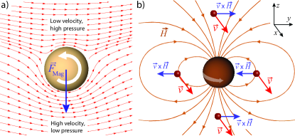
Figure 1: a) Magnus effect in fluid dynamics, as viewed from a spinning body’s frame: the body’s rotation slows down the flow which opposes the body’s surface velocity, while speeding it up otherwise, generating a pressure gradient and a net force $\bm{F}_{{\rm Mag}}$ on the body. b) A gravitational analogue of the Magnus effect? — due to its gravitomagnetic field $\bm{H}$, a spinning body deflects particles of a cloud flowing around it, via the gravitomagnetic “force” $\bm{F}_{{\rm GM}}=M\bm{v}\times\bm{H}$. By naive application of an action-reaction principle, a force on the body orthogonal to its spin and velocity (like the Magnus force) might be expected.

By its very own nature, the fluid-dynamical Magnus force hinges on contact interactions between the spinning body and the fluid. Thus, ordinary Magnus forces cannot exist in the interaction between (i) a fluid and a spinning black hole (BH), or (ii) an ordinary star and dark matter (DM) which only interacts with it via gravity. However, in general relativity any form of energy gravitates and contributes to the gravitational field of bodies. In particular, a spinning body produces a “gravitomagnetic field” CiufoliniWheeler ; if the spinning body is immersed in a fluid, such field deflects the fluid-particles in a direction orthogonal to their velocity, as illustrated in Fig. 1b, seemingly leading to a nonzero “momentum transfer” to the fluid. The question then arises if some backreaction on the body, in the form of a Magnus- (or anti-Magnus)-like force — in the sense of being orthogonal to the flow and to the body’s spin — might arise. Indeed, the existence of such a force, in the same direction of the Magnus effect of fluid dynamics, is strongly suggested by numerical studies of nonaxisymmetric relativistic Bondi-Hoyle accretion onto a Kerr BH Font:1998sc . These studies focused on a fixed background geometry and studied the momentum imparted to the fluid as it accretes or scatters from the BH. A theoretical argument for the existence of such an effect has also been put forth in Ref. Okawa:2014sxa , based on the asymmetric accretion of matter around a spinning BH (i.e, the absorption cross-section being larger for counter- than for corotating particles) — which is but another consequence of the gravitomagnetic “forces”: these are attractive for counterrotating particles, and repulsive for corotating ones, as illustrated in Fig. 1b (for particles in the equatorial plane). Such argument leads however to the prediction of an effect in the direction opposite to the Magnus effect (“anti-Magnus”), thus seemingly at odds with the results in Ref. Font:1998sc . Very recently, and while our work was being completed, there was also an attempt to demonstrate the existence of what, in practice, would amount to such an effect, based both on particle’s absorption and on orbital precessions around a spinning BH Cashen:2016neh (which, again, are gravitomagnetic effects); a force in the direction opposite to the Magnus effect was again suggested. These (conflicting) treatments are however based on loose estimates, not on a concrete computation of the overall gravitomagnetic force exerted by the spinning body on the surrounding matter. Moreover, these are all indirect methods, in which one infers the motion of the body by observing its effect on the cloud, trying then to figure out the backreaction on the body (which, as we shall see, is problematic, since the gravitomagnetic interactions, analogously to the magnetic interactions, do not obey in general an action-reaction law).

One of the purposes of this work is to perform the first concrete and rigorous calculation of this effect. We first take a direct approach — that is, we investigate this effect from the actual equations of motion for spinning bodies in general relativity. These are well established, and known as the Mathisson-Papapetrou (or Mathisson-Papapetrou-Dixon) equations Mathisson:1937zz ; Papapetrou:1951pa ; Dixon1964 ; Dixon:1970zza ; Gralla:2010xg ; Tulczyjew . We will show that a Magnus-type force is a fundamental part of the spin-curvature force, which arises whenever a spinning body moves in a medium with a relative velocity not parallel to its spin axis; it has the same direction as the Magnus force in fluid dynamics, and depends only on the mass-energy current relative to the body, and on the body’s spin angular momentum. Then we also consider the reciprocal problem, rigorously computing the force that the body exerts on the surrounding matter (in the regime where such “force” is defined), correcting and clarifying the earlier results in the literature. These effects have a close parallel in electromagnetism, where an analogous (anti) Magnus effect also arises. For this reason we will start by electromagnetism — and by the classical problem of a magnetic dipole inside a current slab — which will give us insight into the gravitational case.

I.1 Notation and conventions

We use the signature $(-+++)$; $\epsilon_{\alpha\beta\sigma\gamma}\equiv\sqrt{-g}[\alpha\beta\gamma\delta]$ is the Levi-Civita tensor, with the orientation $[1230]=1$ (i.e., in flat spacetime, $\epsilon_{1230}=1$); $\epsilon_{ijk}\equiv\epsilon_{ijk0}$. Greek letters $\alpha$, $\beta$, $\gamma$, … denote 4D spacetime indices, running 0-3; Roman letters $i,j,k,...$ denote spatial indices, running 1-3. The convention for the Riemann tensor is $R_{\ \beta\mu\nu}^{\alpha}=\Gamma_{\beta\nu,\mu}^{\alpha}-\Gamma_{\beta\mu,\nu}^{\alpha}+...$ . $\star$ denotes the Hodge dual: $\star F_{\alpha\beta}\equiv\epsilon_{\alpha\beta}^{\ \ \ \mu\nu}F_{\mu\nu}/2$ for an antisymmetric tensor $F_{\alpha\beta}=F_{[\alpha\beta]}$. Ordinary time derivatives are sometimes denoted by dot: $\dot{X}\equiv\partial X/\partial t$.

I.2 Executive summary

For the busy reader, we briefly outline here the main results of our paper. A spinning body in a gravitational field is acted, in general, by a covariant force $DP^{\alpha}/d\tau$ (the spin-curvature force), deviating it from geodesic motion. Such force can be can be split into the two components

$$\frac{DP^{\alpha}}{d\tau}=F_{{\rm Weyl}}^{\alpha}+F_{{\rm Mag}}^{\alpha}\,,$$ (2)

$$F_{{\rm Weyl}}^{\alpha}\equiv-\mathcal{H}^{\alpha\beta}S_{\beta};\qquad F_{{\rm Mag}}^{\alpha}\equiv 4\pi\epsilon_{\ \beta\sigma\gamma}^{\alpha}J^{\beta}S^{\sigma}U^{\gamma}\ ,$$ (3)

where $U^{\alpha}$ is the body’s 4-velocity, $S^{\alpha}$ its spin angular momentum 4-vector, and $J^{\alpha}=-T^{\alpha\beta}U_{\beta}$ the mass-energy 4-current relative to the body. The force $F_{{\rm Weyl}}^{\alpha}$ is due to the magnetic part of the Weyl tensor, $\mathcal{H}_{\alpha\beta}=\star C_{\alpha\mu\beta\nu}U^{\mu}U^{\nu}$, determined by the details of the system (boundary conditions, etc). The force $F_{{\rm Mag}}^{\alpha}$, which, in the body’s rest frame reads $\bm{F}_{{\rm Mag}}=4\pi\bm{J}\times\bm{S}$, is what we call a gravitational analogue to the Magnus force of fluid dynamics; it arises whenever, relative to the body, there is a spatial mass-energy current $\bm{J}$ not parallel to $\bm{S}$. We argue that (2) is the force that has been attempted to be indirectly computed in the literature Font:1998sc ; Okawa:2014sxa ; Cashen:2016neh , from the effect of a moving BH (or spinning body) on the surrounding matter. We base our claim on a rigorous computation of the reciprocal force exerted by the body on the medium, in the cases where the problem is well posed, and where an action-reaction law can be applied. $F_{{\rm Mag}}^{\alpha}$ and $F_{{\rm Weyl}}^{\alpha}$ are also seen to have direct analogues in the force that an electromagnetic field exerts on a magnetic dipole.

The two components of the force are studied for spinning bodies in (“slab”) toy models, and in some astrophysical setups. For quasi-circular orbits around stationary axisymmetric spacetimes studied — spherical DM halos, BH accretion disks — when $\bm{S}$ lies in the orbital plane, the spin-curvature force takes the form $\bm{F}=A(r)\bm{S}\times\bm{v}$, where the function $A(r)$ is specific to the system. Its Magnus component is similar for all systems, whereas the Weyl component greatly differs. The force $\bm{F}$ causes the orbits to oscillate, and to undergo a secular precession, given by

$$\left\langle\frac{d\bm{L}}{dt}\right\rangle=\bm{\Omega}\times\bm{L};\qquad\bm{\Omega}=\frac{A(r)}{2m}\bm{S}\ .$$

The effect might be detectable in some astrophysical settings, likely candidates are: i) signature in the Milky Way galactic disk: stars or BHs with spin axes nearly parallel to the galactic plane, should be in average more distant from the plane than other bodies; ii) BH binaries where one of the BHs moves in the others’ accretion disk, the secular precession might be detected in gravitational wave measurements in the future, through its impact on the waveforms and emission directions.

In an universe filled with an homogeneous isotropic fluid, described by the FLRW spacetime, representing the large scale structure of the universe, which is conformally flat, we have that $\mathcal{H}^{\alpha\beta}=0\Rightarrow F_{{\rm Weyl}}^{\alpha}=0$, and so the Magnus force $F_{{\rm Mag}}^{\alpha}$ is the only force that acts on a spinning body. It reads, exactly,

$$\bm{F}=-4\pi(\rho+p)(U^{0})^{2}\bm{v}\times\bm{S}$$

It acts on any celestial body that moves with respect to the background fluid with a velocity $\bm{v}\nparallel\bm{S}$, and might possibly be observed in the motion of galaxies with large peculiar velocities $\bm{v}$. Due to the occurrence of the factor $(\rho+p)$, this force acts as a probe for the matter/energy content of the universe (namely for the ratio $\rho/p$, and for the different dark energy candidates). Any mater/energy content gives rise to such gravitational Magnus force, except for dark energy if modeled with a cosmological constant ($\rho=-p$).

II Electromagnetic (anti) Magnus effect

We start with a toy problem borrowed from the electromagnetic interaction. Consider a magnetic dipole within a cloud of charged particles. Is there a Magnus-type force?

The relativistic expression for the force exerted on a magnetic dipole, of magnetic moment 4-vector $\mu^{\alpha}$, placed in a electromagnetic field described by a Faraday tensor $F^{\alpha\beta}$, is Dixon1964 ; Dixon:1970zza ; Gralla:2010xg ; Costa:2012cy

$${\displaystyle\frac{DP^{\alpha}}{d\tau}=B^{\beta\alpha}\mu_{\beta}\equiv F_{{\rm EM}}^{\alpha}};\qquad B_{\alpha\beta}\equiv\star F_{\alpha\mu;\beta}U^{\mu}\,,$$ (4)

where $P^{\alpha}$ is the particle’s 4-momentum, $U^{\alpha}$ its 4-velocity, and $B_{\alpha\beta}$ is the “magnetic tidal tensor” FilipeCosta:2006fz ; Costa:2016iwu as measured in the particle’s rest frame. In the inertial frame momentarily comoving with the particle, the space components of $F_{{\rm EM}}^{\alpha}$ yield the textbook expression

$$\bm{F}_{{\rm EM}}=\nabla(\bm{B}\cdot\bm{\mu})\,.$$ (5)

Taking the projection orthogonal to $U^{\alpha}$ of the Maxwell field equations $F_{\ \ ;\beta}^{\alpha\beta}=4\pi j^{\alpha}$, leads to $B_{[\alpha\beta]}=\star F_{\alpha\beta;\gamma}U^{\gamma}/2-2\pi\epsilon_{\alpha\beta\sigma\gamma}j^{\sigma}U^{\gamma}$ (cf. Eq. (I.3a) in Table I of Ref. Costa:2012cy ), where $j^{\alpha}$ is the current density 4-vector. Therefore

$$B_{\alpha\beta}=B_{(\alpha\beta)}+\frac{1}{2}\star F_{\alpha\beta;\gamma}U^{\gamma}-2\pi\epsilon_{\alpha\beta\sigma\gamma}j^{\sigma}U^{\gamma}\,.$$ (6)

Thus, the magnetic tidal tensor decomposes into three parts: its symmetric part $B_{(\alpha\beta)}$, plus two antisymmetric contributions: the current term $-2\pi\epsilon_{\alpha\beta\sigma\gamma}j^{\sigma}U^{\gamma}$, and the term $\star F_{\alpha\beta;\gamma}U^{\gamma}/2$, which arises when the fields are not covariantly constant along the particle’s worldline (it is related to the laws of electromagnetic induction, as discussed in detail in Costa:2012cy ). The force (4) can then be decomposed as

$$F_{{\rm EM}}^{\alpha}=F_{{\rm Sym}}^{\alpha}+F_{{\rm Mag}}^{\alpha}+F_{{\rm ind}}^{\alpha}\,,$$ (7)

$$F_{{\rm Sym}}^{\alpha}\equiv B^{(\alpha\beta)}\mu_{\beta}\,,\qquad F_{{\rm ind}}^{\alpha}\equiv-\frac{1}{2}\star F_{\ \ ;\gamma}^{\alpha\beta}U^{\gamma}\mu_{\beta}\,,$$ (8)

$$F_{{\rm Mag}}^{\alpha}\equiv 2\pi\epsilon_{\ \beta\sigma\gamma}^{\alpha}U^{\gamma}j^{\sigma}\mu^{\beta}\,.$$ (9)

Let $h_{\ \beta}^{\alpha}$ denote the space projector with respect to $U^{\alpha}$ (projector orthogonal to $U^{\alpha}$),

$$h_{\ \beta}^{\alpha}\equiv U^{\alpha}U_{\beta}+\delta_{\ \beta}^{\alpha}\,.$$ (10)

Since the tensor $\epsilon_{\alpha\beta\sigma\gamma}U^{\gamma}$ automatically projects spatially, in any of its indices, in fact only the projection of $j^{\sigma}$ orthogonal to $U^{\gamma}$, $h_{\ \mu}^{\sigma}j^{\mu}$, contributes to $F_{{\rm Mag}}^{\alpha}$. Physically, $h_{\ \mu}^{\sigma}j^{\mu}$ is the spatial charge current density as measured in the particle’s rest frame. In such frame, the time component of $F_{{\rm Mag}}^{\alpha}$ vanishes, and the space components read

$$\bm{F}_{{\rm Mag}}=2\pi\bm{\mu}\times\bm{j}\ .$$ (11)

This is a force orthogonal to $\bm{\mu}$ and to the spatial current density $\bm{j}$, which we dub electromagnetic “Magnus” force. If the magnetic dipole consists of a spinning, positively (and uniformly) charged body, so that $\bm{\mu}\parallel\bm{S}$, the force $\bm{F}_{{\rm Mag}}$ has a direction opposite to the Magnus force of fluid dynamics (so it is actually “anti-Magnus”). If the body is negatively charged, so that $\bm{\mu}\parallel-\bm{S}$, the force points in the same direction of a Magnus force.

II.1 Example: The force exerted by a current slab on a dipole

The induction component $F_{{\rm ind}}^{\alpha}$ has no gravitational counterpart, as we shall see. Therefore, from now onwards we will not consider it any further. To shed light on the components $F_{{\rm Mag}}^{\alpha}$ and $F_{{\rm Sym}}^{\alpha}$, we consider a simple stationary setup (Exercise 5.14 of Ref. GriffithsBook ): a semi-infinite cloud of charged gas which is infinitely long ($x$ direction) and wide ($z$ direction), but of finite thickness $h$ in the $y$ direction, contained between the planes $y=h/2$ and $y=-h/2$, see Fig. 2.

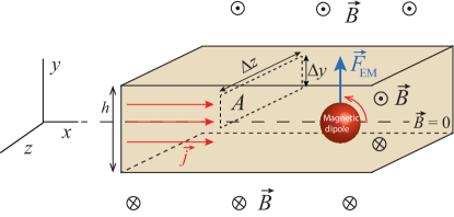
Figure 2: A magnetic dipole $\bm{\mu}=\mu\bm{e}_{z}$ inside a semi-infinite cloud of charged particles flowing in the $\bm{e}_{x}$ direction. The cloud is infinite along the $x$ and $z$ directions, but of finite thickness in the $y$ direction, contained within $-h/2\leq y\leq+h/2$. The magnetic field $\bm{B}$ generated by the cloud points in the positive $z$ direction for $y>0$, and in the negative $z$ direction for $y<0$. $\bm{B}$ has a gradient inside the cloud, whose only nonvanishing component is $B^{z,y}=4\pi j$. Due to that, a force $\bm{F}_{{\rm EM}}=B^{z,y}\mu\bm{e}_{y}=4\pi j\mu\bm{e}_{y}$, pointing upwards, is exerted on the dipole. In this case $\bm{F}_{{\rm{\rm Sym}}}=\bm{F}_{{\rm Mag}}$, so the force is twice the Magnus force: $\bm{F}_{{\rm EM}}=\bm{F}_{{\rm Sym}}+\bm{F}_{{\rm Mag}}=2\bm{F}_{{\rm Mag}}$. Considering instead a cloud finite along $z$, infinite along $x$ and $y$, $\bm{F}_{{\rm Mag}}=2\pi j\mu\bm{e}_{y}$ remains the same, but $\bm{F}_{{\rm Sym}}$ inverts its direction: $\bm{F}_{{\rm{\rm Sym}}}=-\bm{F}_{{\rm Mag}}$, causing the total force to vanish: $\bm{F}_{{\rm EM}}=0$.

Outside the slab, the field is uniform and has opposite directions in either side GriffithsBook . The field at any point inside the cloud is readily obtained by application of the Stokes theorem to the stationary Maxwell-Ampère equation

$$\nabla\times\bm{B}=4\pi\bm{j}\ .$$ (12)

That is, let $A$ be a rectangle in the $z-y$ plane, as illustrated in Fig. 2, with boundary $\partial A$ and normal unit vector $\bm{n}$. By the Stokes theorem

$$\oint_{\partial A}\bm{B}\cdot d\bm{l}=\oint_{A}\nabla\times\bm{B}\cdot\bm{n}dA=4\pi\oint_{A}\bm{j}\cdot\bm{n}dA=4\pi\Delta z\Delta yj\,,$$ (13)

where we took, for the surface $A$, the orientation $\bm{n}\parallel\bm{j}$. By the right-hand-rule and symmetry arguments, $\bm{B}$ is parallel to the slab and orthogonal to $\bm{j}$, pointing in the positive $z$ direction for $y>0$, in the negative $z$ direction for $y<0$, and vanishing at $y=0$. Therefore $\oint_{\partial A}\bm{B}\cdot d\bm{l}=B|_{y=\Delta y}\Delta z$, and so

$$B^{z}(y)=4\pi\Delta yj=4\pi yj\ .$$ (14)

Consider now a magnetic dipole at rest inside the cloud (for instance, the magnetic dipole moment of a spinning charged body), as depicted in Fig. 2. The magnetic field (14) has a gradient inside the cloud, leading to a magnetic tidal tensor $B^{\alpha\beta}$ (as measured by the dipole) whose only nonvanishing component is $B^{zy}=B^{z,y}=4\pi j$. Therefore, the force exerted on the dipole is, cf. Eq. (4),

$$\bm{F}_{{\rm EM}}=B^{ji}\mu_{j}\bm{e}_{i}=B^{zy}\mu_{z}\bm{e}_{y}=4\pi j\mu_{z}\bm{e}_{y}\,.$$ (15)

It consists of the sum of the Magnus force plus the force $\bm{F}_{{\rm Sym}}$ ($\bm{F}_{{\rm ind}}=0$ since the configuration is stationary): $\bm{F}_{{\rm EM}}=\bm{F}_{{\rm Mag}}+\bm{F}_{{\rm Sym}}$,

$$\bm{F}_{{\rm Mag}}=2\pi\bm{\mu}\times\bm{j}=2\pi j(\mu_{z}\bm{e}_{y}-\mu_{y}\bm{e}_{z})$$ (16)

$$\bm{F}_{{\rm Sym}}=B^{(ji)}\mu_{j}\bm{e}_{i}=2\pi j(\mu_{z}\bm{e}_{y}+\mu_{y}\bm{e}_{z})$$ (17)

Equations (15)-(17) yield the forces for a fixed orientation of the slab (orthogonal to the $y$-axis), and an arbitrary $\bm{\mu}$. This is of course physically equivalent to considering instead a magnetic dipole $\bm{\mu}$ with fixed direction, and varying the orientation of the slab; in this framework, taking $\bm{\mu}=\mu\bm{e}_{z}$, two notable cases stand out:

1. Slab finite along $y$ axis, infinite along $x$ and $z$ (see Fig. 2). The Magnus and the “symmetric” forces are equal: $\bm{F}_{{\rm Mag}}=\bm{F}_{{\rm Sym}}=2\pi j\mu\bm{e}_{y}$, so there is a total force along the $y$ direction equaling twice the Magnus force: $\bm{F}_{{\rm EM}}=2\bm{F}_{{\rm Mag}}=4\pi j\mu\bm{e}_{y}$.

2. Slab finite along $z$ axis, infinite along $x$ and $y$ (slab orthogonal to $\bm{\mu}$). The Magnus force remains the same as in case 1; but $\bm{F}_{{\rm Sym}}$ changes to the exact opposite, $\bm{F}_{{\rm Sym}}=-2\pi j\mu\bm{e}_{y}=-\bm{F}_{{\rm Mag}}$. The total force on the dipole now vanishes: $\bm{F}_{{\rm EM}}=0$.

The results in case 2 follow from noting that, for a slab orthogonal to the $z$ axis, $\bm{B}$ is along $y$ and given by $\bm{B}=-4\pi jz\bm{e}_{y}$, leading to a magnetic tidal tensor with only nonvanishing component $B^{yz}=B^{y,z}=-4\pi j$, thus causing $B^{(ij)}$ to globally change sign comparing to case 1. For other orientations of the slab/dipole, the forces $\bm{F}_{{\rm Sym}}$ and $\bm{F}_{{\rm Mag}}$ are not collinear. When $\bm{\mu}$ coincides with an eigenvector of the matrix $B^{(ij)}$, they are actually orthogonal; in the slab in Fig. 2 (orthogonal to the $y$-axis), that is the case for $\bm{\mu}=\mu(\bm{e}_{y}+\bm{e}_{z})/\sqrt{2}$ and $\bm{\mu}=\mu(\bm{e}_{z}-\bm{e}_{y})/\sqrt{2}$ (the third eigenvector of $B^{(ij)}$, $\bm{\mu}=\mu\bm{e}_{x}$, has zero eigenvalue and leads to $\bm{F}_{{\rm Mag}}=\bm{F}_{{\rm{\rm Sym}}}=0$).

Notice that neither the field $\bm{B}$ at any point inside the cloud, nor its gradient, or the force (15), depend on the precise width $h$ of the cloud; in particular, they remain the same in the limit $h\rightarrow\infty$. The role of considering (at least in a first moment) a finite $h$ is to fix the direction of $\bm{B}$. Equation (12), together with the problem’s symmetries, then fully fix $\bm{B}$ via Eq. (13) and, therefore, $\bm{F}_{{\rm Sym}}$. Taking the limit $h\rightarrow\infty$ in cases 1-2 above yields two different ways of constructing an infinite current cloud, each of them leading to a different $\bm{B}$ and force on the dipole (the situation is analogous to the “paradoxes” of the electric field of a uniform, infinite charge distribution, or of the Newtonian gravitational field of a uniform, infinite mass distribution, see Sec. III.2.3). Had one started with a cloud about which all one is told is that it is infinite in all directions, it would not be possible to set up the boundary conditions needed to solve the Maxwell-Ampère equation (12), so the question of which is the magnetic field (thus the force the dipole) would have no answer.

II.2 Reciprocal problem: The force exerted by the dipole on the slab

There have been attempts at understanding and quantifying the gravitational analogue of the Magnus effect Okawa:2014sxa ; Cashen:2016neh . However, in these works, the force on the spinning body was inferred from its effect on the cloud, by guessing its back reaction on the body. Here we will start by computing it rigorously in the electromagnetic analogue, i.e., the reciprocal of the problem considered above: the force exerted by the magnetic dipole on the cloud. It is given by the integral

$$\bm{F}_{{\rm dip,cloud}}=\int_{{\rm cloud}}\bm{j}\times\bm{B}_{{\rm dip}}d^{3}x=\bm{j}\times\int_{{\rm cloud}}\bm{B}_{{\rm dip}}d^{3}x\ .$$ (18)

Consider a sphere completely enclosing the magnetic dipole, and let $R$ be its radius; we may then split

$$\bm{F}_{{\rm dip,cloud}}=\bm{j}\times\int_{r\leq R}\bm{B}_{{\rm dip}}d^{3}x+\bm{j}\times\int_{r>R}\bm{B}_{{\rm dip}}d^{3}x$$ (19)

The interior integral yields

$$\int_{r\leq R}\bm{B}_{{\rm dip}}d^{3}x=\frac{8\pi}{3}\bm{\mu}\ ,$$ (20)

as explained in detail in pp. 187-188 of Jackson:1998nia . The magnetic field in any region exterior to the dipole is (e.g. GriffithsBook ; Jackson:1998nia )

$$\bm{B}_{{\rm dip}}|_{r>R}=-\frac{\bm{\mu}}{r^{3}}+\frac{3(\bm{\mu}\cdot\bm{r})\bm{r}}{r^{5}}\ .$$ (21)

For the setup in Fig. 2 (slab orthogonal to the $y$-axis, $\bm{\mu}=\mu\bm{e}_{z}$), and considering a spherical coordinate system where $z^{2}/r^{2}=\cos^{2}\theta$ and the plane $y=h/2$ is given by the equation $r=h/(2\sin\theta\sin\phi)$, the exterior integral becomes

$$\int_{r>R}\bm{B}_{{\rm dip}}d^{3}x=2\mu\bm{e}_{z}$$ (22)

$$\times \int_{0}^{\pi}d\theta\int_{0}^{\pi}d\phi\int_{R}^{\beta}dr\frac{3\cos^{2}\theta-1}{r}\sin\theta=\frac{4}{3}\pi\mu\bm{e}_{z}\,,$$

with $\beta=h/(2\sin\theta\sin\phi)$. Substituting Eqs. (20) and (22) into (19), and comparing to Eq. (15), we see that

$$\bm{F}_{{\rm dip,cloud}}=-4\pi j\mu\bm{e}_{y}=-\bm{F}_{{\rm EM}}\equiv-\bm{F}_{{\rm cloud,dip}}\ ,$$ (23)

i.e., the force exerted by the dipole on the cloud indeed equals minus the force exerted by the cloud on the dipole. It is however important to note that this occurs because one is dealing here with magnetostatics; for general electromagnetic interactions do not obey the action-reaction law (in the sense of a reaction force equaling minus the action). This is exemplified in Appendix B.1. In particular it is so for the interaction of the dipole with individual particles of the cloud.

If one considers instead a slab orthogonal to the $z$ axis (contained within $-h/2\leq z\leq+h/2$), and noting that the plane $z=h/2$ is given by $r=h/(2\cos\theta)$, one obtains $\int_{r>R}\bm{B}_{{\rm dip}}d^{3}x=-(8\pi/3)\mu\bm{e}_{z}$, which exactly cancels out the interior integral (20), leading to a zero force on the cloud: $\bm{F}_{{\rm dip,cloud}}=0$ (matching, again, its reciprocal).

Just like in the reciprocal problem, the results do not depend on the width $h$ of the slabs, so taking the limit $h\rightarrow\infty$ of the slabs orthogonal to $y$ and to $z$ are two different ways of obtaining equally infinite clouds, but on which very different forces are exerted. Here the issue does not boil down to a problem of boundary conditions for PDE’s (as was the case for $\bm{B}$ in Sec. II.1); it comes about instead in another fundamental mathematical principle (Fubini’s theorem Fubini ; PeterWalker ): the multiple integral of a function which is not absolutely convergent, depends in general on the way the integration is performed. This is discussed in detail in Appendix A. It tells us that, like its reciprocal, $\bm{F}_{{\rm dip,cloud}}$ is not a well defined quantity for an infinite cloud.

III Gravitational Magnus effect

Contrary to idealized point (“monopole”) particles, “real,” extended bodies, endowed with a multipole structure, do not move along geodesics in a gravitational field. This is because the curvature tensor couples to the multipole moments of the body’s energy momentum tensor $T^{\alpha\beta}$ (much like in the way the electromagnetic field couples to the multipole moments of the current 4-vector $j^{\alpha}$). In a multiple scheme, the first correction to geodesic motion arises when one considers pole-dipole spinning particles, i.e., particles whose only multipole moments of $T^{\alpha\beta}$ relevant to the equations of motion are the momentum $P^{\alpha}$ and the spin tensor $S^{\alpha\beta}$ (see e.g. Dixon1964 ; Dixon:1970zza ; Costa:2014nta for their definitions in a curved spacetime). In this case the equations of motion that follow from the conservation laws $T_{\ \ \ ;\beta}^{\alpha\beta}=0$ are the so-called Mathisson-Papapetrou (or Mathisson-Papapetrou-Dixon) equations Mathisson:1937zz ; Papapetrou:1951pa ; Dixon1964 ; Dixon:1970zza ; Gralla:2010xg ; Tulczyjew . According to these equations, a spinning body experiences a force, the so called spin-curvature force, when placed in a gravitational field. It is described by

$$\frac{DP^{\alpha}}{d\tau} = -\frac{1}{2}R_{\ \beta\mu\nu}^{\alpha}S^{\mu\nu}U^{\beta}\ \equiv\ F^{\alpha}\,,$$ (24)

where $U^{\alpha}=dx^{\alpha}/d\tau$ is the body’s 4-velocity (that is, the tangent vector to its center of mass worldline). This is a physical, covariant force (as manifest in the covariant derivative operator $D/d\tau\equiv U^{\alpha}\nabla_{\alpha}$), which causes the body to deviate from geodesic motion. Under the so-called Mathisson-Pirani Mathisson:1937zz ; Pirani:1956tn spin condition $S^{\alpha\beta}U_{\beta}=0$, one may write $S^{\mu\nu}=\epsilon^{\mu\nu\tau\lambda}S_{\tau}U_{\lambda}$, where $S^{\alpha}\equiv\epsilon_{\ \beta\mu\nu}^{\alpha}U^{\beta}S^{\mu\nu}/2$ is the spin 4-vector [whose components in an orthonormal frame comoving with the body are $S^{\alpha}=(0,\bm{S})$]. Substituting in (24), leads to Costa:2012cy ; FilipeCosta:2006fz ,

$$F^{\alpha}=\frac{DP^{\alpha}}{d\tau}=-\mathbb{H}^{\beta\alpha}S_{\beta}\,,$$ (25)

where

$$\mathbb{H}_{\alpha\beta}\equiv\star R_{\alpha\mu\beta\nu}U^{\mu}U^{\nu}=\frac{1}{2}\epsilon_{\alpha\mu}^{\ \ \ \ \lambda\tau}R_{\lambda\tau\beta\nu}U^{\mu}U^{\nu}\,,$$ (26)

is the “gravitomagnetic tidal tensor” (or “magnetic part” of the Riemann tensor, e.g. Dadhich:1999eh ) as measured by an observer comoving with the particle. Using the decomposition of the Riemann tensor in terms of the Weyl ($C_{\alpha\beta\gamma\delta}$) and Ricci tensors (e.g. Eq. (2.79) of Ref. EllisMaartensMacCallum ),

$$R_{\ \ \gamma\delta}^{\alpha\beta} =C_{\ \ \gamma\delta}^{\alpha\beta}+2\delta_{[\gamma}^{[\alpha}R^{\beta]}{}_{\delta]}-\frac{1}{3}R\delta_{[\gamma}^{\alpha}\delta_{\delta]}^{\beta}\ ,$$ (27)

we may decompose $\mathbb{H}_{\alpha\beta}$ as

$$\mathbb{H}_{\alpha\beta}=\mathbb{H}_{(\alpha\beta)}+\mathbb{H}_{[\alpha\beta]}=\mathcal{H}_{\alpha\beta}+\frac{1}{2}\epsilon_{\alpha\beta\sigma\gamma}U^{\gamma}R^{\sigma\lambda}U_{\lambda}\ ,$$ (28)

where the symmetric tensor $\mathcal{H}_{\alpha\beta}=\mathbb{H}_{(\alpha\beta)}$ is the magnetic part of the Weyl tensor, $\mathcal{H}_{\alpha\beta}\equiv\star C_{\alpha\mu\beta\nu}U^{\mu}U^{\nu}$. Using the Einstein field equations

$$R_{\mu\nu}=8\pi(T_{\mu\nu}-\frac{1}{2}g_{\mu\nu}T_{\,\,\,\alpha}^{\alpha})+\Lambda g_{\alpha\beta}\ ,$$ (29)

this becomes (cf. e.g. Eq. (I.3b) of Table I of Costa:2012cy )

$$\mathbb{H}_{\alpha\beta}=\mathbb{H}_{(\alpha\beta)}+\mathbb{H}_{[\alpha\beta]}=\mathcal{H}_{\alpha\beta}-4\pi\epsilon_{\alpha\beta\sigma\gamma}U^{\gamma}J^{\sigma}\,,$$ (30)

where $J^{\alpha}\equiv-T^{\alpha\beta}U_{\beta}$ is the mass/energy current 4-vector as measured by an observer of 4-velocity $U^{\alpha}$ (comoving with the particle, in this case). We thus can write

$$F^{\alpha}=-\mathcal{H}^{\alpha\beta}S_{\beta}+4\pi\epsilon_{\ \beta\sigma\gamma}^{\alpha}J^{\beta}S^{\sigma}U^{\gamma}=F_{{\rm Weyl}}^{\alpha}+F_{{\rm Mag}}^{\alpha}\ ,$$ (31)

where

$$F_{{\rm Mag}}^{\alpha} \equiv 4\pi\epsilon_{\ \beta\sigma\gamma}^{\alpha}U^{\gamma}J^{\beta}S^{\sigma}\ ,$$ (32)

$$F_{{\rm Weyl}}^{\alpha} \equiv-\mathcal{H}^{\alpha\beta}S_{\beta}\ .$$ (33)

Since the tensor $\epsilon_{\alpha\beta\sigma\gamma}U^{\gamma}$ automatically projects spatially (in any of its free indices), only the projection of $J^{\beta}$ orthogonal to $U^{\gamma}$, $h_{\ \mu}^{\beta}J^{\mu}$ [see Eq. (10)], contributes to $F_{{\rm Mag}}^{\alpha}$.

Equations (31)-(33) thus tell us that the spin-curvature force splits into two parts: $F_{{\rm Weyl}}^{\alpha}$, which is due to the magnetic part of the Weyl tensor, and is analogous (to some extent) to the “symmetric force” $F_{{\rm Sym}}^{\alpha}$ of electromagnetism, Eq. (8). The second part is $F_{{\rm Mag}}^{\alpha}$ which is nonvanishing whenever, relative to the body, there is a spatial mass-energy current $h_{\ \mu}^{\beta}J^{\mu}$ not parallel to $S^{\alpha}$. In the body’s rest frame, we have

$$\bm{F}_{{\rm Mag}}=4\pi\bm{J}\times\bm{S}\,,$$ (34)

thus $F_{{\rm Mag}}^{\alpha}$ is what one would call a gravitational analogue of the Magnus effect in fluid dynamics, since

i) it arises whenever the body rotates and moves in a medium with a relative velocity not parallel to its spin axis (that is, when there is a spatial mass-energy current density $\bm{J}$ relative to the body, such that $\bm{S}\nparallel\bm{J}$);

ii) the force is orthogonal to both the axis of rotation of the body (i.e. to $\bm{S}$) and to the current density $\bm{J}$, like in an ordinary Magnus effect; moreover, it points precisely in the same direction of the latter.

Notice that Eq. (31) is a fully general equation that can be applied to any system, and that the “Magnus force” $F_{{\rm Mag}}^{\alpha}$ depends only on $U^{\alpha}$, $S^{\alpha}$, and the local $J^{\alpha}$, and not on any further detail of the system. The force $F_{{\rm Weyl}}^{\alpha}$, by contrast, strongly depends on the details of the system (as exemplified in Sec. III.2 below). This can be traced back to the fact that $F_{{\rm Mag}}^{\alpha}$ comes from the Ricci part of the curvature, totally fixed by the energy-momentum tensor $T^{\alpha\beta}$ of the local sources via the Einstein Eqs. (29), whereas the Weyl tensor describes the “free gravitational field,” which does not couple to the sources via algebraic equations, only through differential ones (the differential Bianchi identities MaartensBasset1997 ; EllisMaartensMacCallum ), being thus determined not by the value of $T^{\alpha\beta}$ at a point, but by conditions elsewhere EllisMaartensMacCallum .

Note also that, in general, $\bm{F}_{{\rm Mag}}$ is not the total force in the direction orthogonal to $\bm{S}$ and $\bm{J}$; $F_{{\rm Weyl}}^{\alpha}$ may also have a component along it.

III.1 Post-Newtonian approximation

Up to here, we used no approximations in the description of the gravitational forces. For most astrophysical systems, however, no exact solutions of the Einstein field equations are known; in these cases we use the post-Newtonian (PN) approximation to general relativity. This expansion can be framed in different — equivalent — ways; namely, by counting powers of $c$ Damour:1990pi ; WillPoissonBook or in terms of a dimensionless parameter Misner:1974qy ; Costa:2016iwu ; Will:1993ns ; Kaplan:2009 ; Binietal1994 . Here we will follow the latter, which consists of making an expansion in terms of a small dimensionless parameter $\epsilon$, such that $U\sim\epsilon^{2}$ and $v\lesssim\epsilon$, where $U$ is (minus) the Newtonian potential, and $v$ is the velocity of the bodies (notice that, for bodies in bounded orbits, $v\sim\sqrt{U}$). In terms of “forces,” the Newtonian force $m\nabla U$ is taken to be of zeroth PN order (0PN), and each factor $\epsilon^{2}$ amounts to a unity increase of the PN order. Time derivatives increase the degree of smallness of a quantity by a factor $\epsilon$; for example, $\partial U/\partial t\sim Uv\sim\epsilon U$. The 1PN expansion consists of keeping terms up to $O(\epsilon^{4})\equiv O({4})$ in the equations of motion Will:1993ns . This amounts to considering a metric of the form Damour:1990pi ; Kaplan:2009

$$g_{00} =-1+2w-2w^{2}+O({6})$$

$$g_{i0} =\mathcal{A}_{i}+O({5});\qquad g_{ij}=\delta_{ij}\left(1+2U\right)+O({4})\,,$$ (35)

where $\bm{\mathcal{A}}$ is the “gravitomagnetic vector potential” and the scalar $w$ consists of the sum of $U$ plus nonlinear terms of order $\epsilon^{4}$, $w=U+O({4})$. For the computation of the space part of the force (25), the components $\mathbb{H}_{ij}$, $\mathbb{H}_{0i}$, of the gravitomagnetic tidal tensor (26) are needed. Using $U^{\alpha}=U^{0}(1,\bm{v})$ and the 1PN Christoffel symbols in e.g. Eqs. (8.15) of Ref. WillPoissonBook , they read

$$\mathbb{H}_{ij}= -\frac{1}{2}\epsilon_{i}^{\ lk}\mathcal{A}_{k,lj}-\epsilon_{ij}^{\ \ k}\dot{U}_{,k}+2\epsilon_{i}^{\ km}v_{k}U_{,jm}$$

$$-\epsilon_{ij}^{\ \ m}U_{,km}v^{k}+O({5})\,,$$ (36)

$$\mathbb{H}_{0i}= \epsilon_{ij}^{\ \ l}\dot{U}_{,l}v^{j}+\frac{1}{2}\epsilon_{j}^{\,\,\,lk}\mathcal{A}_{k,li}v^{j}+\epsilon_{\ ji}^{l}U_{,lk}v^{j}v^{k}\ (=O({4}))\,,$$ (37)

where dot denotes ordinary time derivative, $\partial/\partial t$. Equation (36) is a generalization of Eq. (3.41) of Ref. Damour:1990pi for nonvacuum, and for the general case that the observer measuring the tensor $\mathbb{H}_{\alpha\beta}$ moves (i.e., $\bm{v}\neq 0$). It is useful to write $\mathbb{H}_{ij}$ in terms of the gravitoelectric ($\bm{G}$) and gravitomagnetic ($\bm{H}$) fields, defined by Costa:2016iwu ; Kaplan:2009 ; Damour:1990pi

$$\bm{G}=\nabla w-\dot{\bm{\mathcal{A}}}+O({6})\,,\quad\bm{H}=\nabla\times\bm{\mathcal{A}}+O({5})\ .$$ (38)

The reason for these denominations is that these fields play in gravity a role analogous to the electric and magnetic fields. One has then

$$\mathbb{H}_{ij} =-\frac{1}{2}H_{i,j}-\epsilon_{ijk}\dot{G^{k}}+2\epsilon_{i}^{\ km}v_{k}G_{j,m}$$

$$-\epsilon_{ij}^{\ \ m}G_{k,m}v^{k}+O({5})\ .$$ (39)

Noting that the orthogonality relation $S_{\alpha}U^{\alpha}=0$ implies $S_{0}=-S_{i}v^{i}=O({1})$, it follows, from Eqs. (25) and (37), that $F^{j}=-\mathbb{H}^{ij}S_{i}-\mathbb{H}^{0j}S_{0}=-\mathbb{H}^{ij}S_{i}+O({5})$, and so the 1PN spin-curvature force reads

$$F^{j} =\frac{1}{2}H^{i,j}S_{i}-(\bm{S}\times\dot{\bm{G}})^{j}-2\epsilon^{ikm}v_{k}G_{\ ,m}^{j}S_{i}$$

$$-\epsilon^{jim}G_{k,m}v^{k}S_{i}+O({5})\ .$$ (40)

Its Magnus and Weyl components, Eqs. (32)-(33), are

$$F_{{\rm Mag}}^{i}= \ 4\pi\epsilon_{\ jk}^{i}S^{k}(T^{0j}-\rho v^{j})+O({5})\ ,$$ (41)

$$F_{{\rm Weyl}}^{i}= \ -\mathcal{H}^{ij}S_{j}+O({5})$$ (42)

$$= \ \frac{1}{2}H^{(i,j)}S_{j}-2\epsilon_{\ km}^{(i}G^{j),m}v^{k}S_{j}+O({5})\ ;$$ (43)

where for $\rho$ one can take the mass/energy density as measured either in the body’s rest frame, or in the PN background frame (the distinction is immaterial in Eq. (41), to the accuracy at hand). Notice that $T^{0j}-\rho v^{j}=h_{\ \beta}^{j}J^{\beta}$ [see Eq. (10)] is indeed the spatial mass-energy current with respect to the body’s rest frame ($T^{0j}$, in turn, yields the spatial mass-energy current as measured in the PN frame).

To obtain the coordinate acceleration of a spinning test body, we first note that, under the Mathisson-Pirani spin condition, the relation between the particle’s 4-momentum $P^{\alpha}$ and its 4-velocity is (e.g. Costa:2014nta ) $P^{\alpha}=mU^{\alpha}+S^{\alpha\beta}a_{\beta}$, where $m\equiv-P^{\alpha}U_{\alpha}$ is the proper mass, which is a constant, $a^{\alpha}\equiv DU^{\alpha}/d\tau$ the covariant acceleration, and the term $S^{\alpha\beta}a_{\beta}$ is the so-called “hidden momentum” Gralla:2010xg ; Costa:2012cy ; Costa:2014nta . In the post-Newtonian regime one can neglect the hidden momentum, leading to the acceleration equation $ma^{\alpha}\simeq DP^{\alpha}/d\tau\equiv F^{\alpha}$. Using $DU^{\alpha}/d\tau=d^{2}x^{\alpha}/d\tau^{2}+\Gamma_{\beta\gamma}^{\alpha}U^{\beta}U^{\gamma}$ and $d/d\tau=(dt/d\tau)d/dt$, where $t$ is the coordinate time, one gets, after some algebra,

$$m\frac{d^{2}x^{i}}{dt^{2}}=F_{{\rm I}}^{i}+F^{i}+O({5})\ ,$$ (44)

where

$$F_{{\rm I}}^{i}=m\left[\frac{dx^{i}}{dt}\Gamma_{\beta\gamma}^{0}-\Gamma_{\beta\gamma}^{i}\right]\frac{dx^{\beta}}{dt}\frac{dx^{\gamma}}{dt}$$ (45)

is the inertial “force” already present in the geodesic equation for a nonspinning point particle: $d^{2}x^{i}/dt^{2}=F_{{\rm I}}^{i}/m$ (cf. e.g. Eq. (8.14) of WillPoissonBook ). Using, again, the 1PN Christoffel symbols in Eqs. (8.15) of WillPoissonBook , yields

$$\frac{\bm{F}_{{\rm I}}}{m}=(1+v^{2}-2U)\bm{G}+\bm{v}\times\bm{H}-3\dot{U}\bm{v}-4(\bm{G}\cdot\bm{v})\bm{v}+O({6})\ .$$ (46)

Equation (44) is a general expression for the coordinate acceleration of a spinning particle in a gravitational field, accurate to 1PN order.

III.2 A cloud “slab”

III.2.1 The Magnus force on spinning objects

Before moving on to more realistic scenarios, we start by investigating the gravitational Magnus force, in the PN approximation, for the gravitational analogue of the electromagnetic system in Sec. II.1. In particular, we consider a spinning body (for example, a BH) inside a medium flowing in the $\bm{e}_{x}$ direction, that we assume to be infinitely long and wide (in the $x$ and $z$ directions), but of finite thickness $h$ ($y$ direction), contained within the planes $-h/2\leq y\leq h/2$. The system is depicted in Fig. 3.

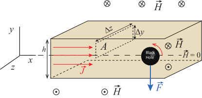
Figure 3: A spinning body (e.g., a BH), with $\bm{S}=S\bm{e}_{z}$, inside a massive cloud flowing in the $\bm{e}_{x}$ direction. The cloud is infinite along $x$ and $z$, and finite along the $y$-axis, contained within $-h/2\leq y\leq h/2$. The vector $\bm{H}$ is the gravitomagnetic field generated by the cloud; it points in the negative (positive) $z$ direction for $y>0$ ($<0$). It has a gradient inside the cloud, whose only nonvanishing component is $H^{z,y}=-16\pi J$; due to that, a spin-curvature force $\bm{F}=(1/2)H^{z,y}S\bm{e}_{y}=-8\pi JS\bm{e}_{y}$, pointing downwards, is exerted on the body. In this case $\bm{F}_{{\rm Mag}}=\bm{F}_{{\rm Weyl}}$, so the total force is twice the Magnus force: $\bm{F}=\bm{F}_{{\rm Mag}}+\bm{F}_{{\rm Weyl}}=2\bm{F}_{{\rm Mag}}$. Considering instead a cloud finite along $z$, and infinite along $x$ and $y$, $\bm{F}_{{\rm Mag}}=-4\pi JS\bm{e}_{y}$ remains the same, but $\bm{F}_{{\rm Weyl}}$ changes to the exact opposite: $\bm{F}_{{\rm Weyl}}=-\bm{F}_{{\rm Mag}}$, causing the total spin-curvature force to vanish: $\bm{F}=0$.

The Einstein field equations yield a gravitational analogue to the Maxwell-Ampère law (12), as we shall now see. For the metric (35), the Ricci tensor component $R_{0i}=(\nabla\times H)_{i}/2-2\dot{\bm{G}}+O({5})$, where $\bm{H}$ is the gravitomagnetic field as defined by Eq. (38). On the other hand, from the Einstein equations (29), we have that $R_{0i}=8\pi T_{0i}+O({5})$. Equating the two expressions, and taking the special case of stationary setups, we have (cf. e.g. Eq. (2.6d) of Ref. Kaplan:2009 )

$$\nabla\times\bm{H}=-16\pi\bm{J}\ ,$$ (47)

where we noted that $T^{0i}=J^{i}+O({5})$, and $J^{\alpha}=-T^{\alpha\beta}u_{\beta}$ is the mass/energy current as measured by the reference observers $u^{\alpha}=u^{0}\delta_{0}^{\alpha}$ [at rest in the coordinate system of (35)]. This equation resembles very closely Eq. (12). For a system analogous to that in Fig. 2 — a cloud of matter passing through a spinning body — an entirely analogous reasoning to that leading to Eq. (14) applies here to obtain the gravitomagnetic field

$$\bm{H}=H^{z}(y)\bm{e}_{z}=-16\pi yJ\bm{e}_{z}\,.$$ (48)

This solution is formally similar to the magnetic field in Eq. (14), apart from the different factor and sign. For a spinning body at rest in a stationary gravitational field, the spin-curvature force, Eq. (40), reduces to

$$F^{i}=\frac{1}{2}H^{j,i}S_{j}\qquad\Leftrightarrow\qquad\bm{F}=\dfrac{1}{2}\nabla(\bm{H}\cdot\bm{S})\,,$$ (49)

(cf. e.g. Eq. (4) of Wald:1972sz ), similar to the dipole force (15). Hence, due to the gradient of $\bm{H}$, whose only nonvanishing component $H^{i,j}$ is $H^{z,y}=-16\pi J$, a force $\bm{F}$ is exerted on a spinning body at rest inside the cloud, given by

$$\bm{F}=-8\pi JS_{z}\bm{e}_{y}\ .$$ (50)

It is thus along the $y$ direction, pointing downwards, in the same direction of an ordinary Magnus effect (and opposite to the electromagnetic analogue). This force consists of the sum of the Magnus force plus the Weyl force: $\bm{F}=\bm{F}_{{\rm Mag}}+\bm{F}_{{\rm Weyl}}$,

$$\bm{F}_{{\rm Mag}}=4\pi\bm{J}\times\bm{S}=4\pi J(S_{y}\bm{e}_{z}-S_{z}\bm{e}_{y})\,,$$ (51)

$$\bm{F}_{{\rm Weyl}}=-\mathcal{H}^{ij}\mu_{j}\bm{e}_{i}=-4\pi J(S_{z}\bm{e}_{y}+S_{y}\bm{e}_{z})\,.$$ (52)

Here, $\mathcal{H}^{ij}=\mathbb{H}^{(ij)}=-H^{(i,j)}/2$, and its nonvanishing components are $\mathcal{H}^{zy}=\mathcal{H}^{yz}=4\pi J$. Again, Eqs. (50)-(52) yield the forces for a fixed orientation of the slab (orthogonal to the $y$-axis), and an arbitrary $\bm{S}$. Of course, this is physically equivalent to considering instead a body with fixed spin direction, and varying the orientation of the slab; choosing $\bm{S}=S\bm{e}_{z}$, one can make formally similar statements to those in Sec. II.1, by replacing $\bm{F}_{{\rm Sym}}$ by $\bm{F}_{{\rm Weyl}}$. Namely, the two notable cases arise:

1. Cloud finite along the $y$-axis, infinite along $x$ and $z$ (Fig. 3). The Magnus force $\bm{F}_{{\rm Mag}}$ equals the Weyl force: $\bm{F}_{{\rm Mag}}=\bm{F}_{{\rm Weyl}}=-4\pi JS\bm{e}_{y}$, so there is a total force downwards which is twice the Magnus force: $\bm{F}=2\bm{F}_{{\rm Mag}}=-8\pi JS\bm{e}_{y}$.

2. Cloud finite along $z$, infinite along $x$ and $y$ (i.e., slab orthogonal to $\bm{S}$). The Magnus force $\bm{F}_{{\rm Mag}}$ remains the same as in case 1; the Weyl force is now exactly opposite to the Magnus force: $\bm{F}_{{\rm Weyl}}=4\pi JS\bm{e}_{y}=-\bm{F}_{{\rm Mag}}$, so the total spin-curvature force vanishes: $\bm{F}=\bm{F}_{{\rm Mag}}+\bm{F}_{{\rm Weyl}}=0$.

In case 2 we noted that, for a slab orthogonal to the $z$ axis, $\bm{H}=16\pi Jz\bm{e}_{y}$, and so the magnetic part of the Weyl tensor $\mathcal{H}^{ij}$ changes sign comparing to the setup in Fig. 3: $\mathcal{H}^{zy}=\mathcal{H}^{yz}=-4\pi J$. For other orientations of the slab/$\bm{S}$, the Weyl and Magnus forces are not parallel. When $\bm{S}$ coincides with an eigenvector of the magnetic part of the Weyl tensor $\mathcal{H}^{ij}$, $\bm{F}_{{\rm Weyl}}\propto\bm{S}$, being therefore orthogonal to $\bm{F}_{{\rm Mag}}$. For the cloud in Fig. 3 (orthogonal to the $y$-axis), this is the case for $\bm{S}=S(\bm{e}_{y}+\bm{e}_{z})/\sqrt{2}$ and $\bm{S}=S(\bm{e}_{z}-\bm{e}_{y})/\sqrt{2}$ (the third eigenvector of $\mathcal{H}^{ij}$, $\bm{S}=S\bm{e}_{x}$, has zero eigenvalue and leads to $\bm{F}_{{\rm Mag}}=\bm{F}_{{\rm{\rm Weyl}}}=0$). Cases 1-2 sharply illustrate the contrast between the two parts of the spin curvature force: on the one hand the Magnus force $\bm{F}_{{\rm Mag}}$, which depends only on $\bm{S}$ and on the local mass-density current $\bm{J}$, and is therefore the same regardless of the boundary; and, on the other hand, the Weyl force, which is determined by the details of the system, namely the direction along which this cloud model has a finite width $h$. Similarly to the electromagnetic case, neither $\bm{H}$ at any point inside the cloud (or its gradient $H^{i,j}$), nor $\bm{F}_{{\rm Weyl}}$, depend on the precise value of $h$; the role of its finiteness boils down to fixing the direction of $\bm{H}$. Equation (47), together with the problem’s symmetries, then fully fix $\bm{H}$ (analogously to the situation for $\bm{B}$ in Sec. II.1). One can then say that, in this example, the magnetic part of the Weyl tensor, $\mathcal{H}_{ij}=\mathbb{H}_{(ij)}$ (and therefore $\bm{F}_{{\rm Weyl}}$), is fixed by the boundary, whereas antisymmetric part of the gravitomagnetic tidal tensor, $\mathbb{H}_{[ij]}$, depends only on the local mass current density $\bm{J}$, cf. Eq. (30).

In general one is interested in the total force $\bm{F}=\bm{F}_{{\rm Mag}}+\bm{F}_{{\rm Weyl}}$ (for it is what determines the body’s motion); the dependence of $\bm{F}_{{\rm Weyl}}$ on the details/boundary conditions of the system shown by the results above hints at the importance of appropriately modeling the astrophysical systems of interest.

III.2.2 The force exerted by the body on the cloud

Previous approaches in the literature attempted to compute the gravitational Magnus force by inferring it from its reciprocal – the force exerted by the body on the cloud Okawa:2014sxa ; Cashen:2016neh . Unfortunately, these attempts were not based on concrete computations of such force, but on estimates which are either not complete (and thereby misleading) or rigorous, and turn out in fact to yield incorrect conclusions (see Sec. III.2.3 and Appendix B.2.1 below for details). In this section we shall rigorously compute, in the framework of the PN approximation, the “force” exerted by the spinning body on the cloud for the setups considered above.

In the first PN approximation, the geodesic equation for a point particle of coordinate velocity $\bm{v}=d\bm{x}/dt$ can be written as $d\bm{v}/dt=\bm{F}_{{\rm I}}/m$, with $\bm{F}_{{\rm I}}$ given by Eq. (46). This equation exhibits formal similarities with the Lorentz force law; namely the gravitomagnetic “force” $m\bm{v}\times\bm{H}$, analogous to the magnetic force $q\bm{v}\times\bm{B}$. The total gravitomagnetic force exerted by the spinning body on the cloud is the sum of the force exerted in each of its individual particles, given by the integral

$$\bm{F}_{{\rm body,cloud}} =\int_{{\rm cloud}}\bm{J}\times\bm{H}_{{\rm body}}d^{3}x$$ (53)

$$=\bm{J}\times\int_{r\leq R}\bm{H}_{{\rm body}}d^{3}x+\bm{J}\times\int_{r>R}\bm{H}_{{\rm body}}d^{3}x$$

where $\bm{H}_{{\rm body}}$ is the gravitomagnetic field generated by the spinning body. Equation (47), formally similar to (12) up to a factor $-4$, implies that

$$\int_{r\leq R}\bm{H}_{{\rm body}}d^{3}x=-\frac{16\pi}{3}\bm{S}$$ (54)

and that the exterior gravitomagnetic field is (cf. e.g. CiufoliniWheeler ; Costa:2015hlh )

$$\bm{H}_{{\rm body}}|_{r>R}=2\frac{\bm{S}}{r^{3}}-6\frac{(\bm{S}\cdot\bm{r})\bm{r}}{r^{5}}\ ,$$ (55)

analogous, up to a factor -2, to (20) and (21), respectively. Therefore, for $\bm{S}=S\bm{e}_{z}$, and a slab finite in the $y$ direction (contained within $-h/2<y<h/2$), as depicted in Fig. 3, an integration analogous to (22) leads to

$$\bm{F}_{{\rm body,cloud}}=8\pi JS\bm{e}_{y}=-\bm{F}\equiv-\bm{F}_{{\rm cloud,body}}\ ,$$

i.e., minus the force exerted by the slab on the body, Eq. (50), satisfying an action-reaction law. For a slab finite in the $z$ direction (contained within $-h/2<z<h/2$), like in the electromagnetic analogue the force vanishes: $\bm{F}_{{\rm body,cloud}}=0$, matching its reciprocal.

Several remarks must however be made on this result. First we note that, unlike the spin-curvature force $\bm{F}\equiv\bm{F}_{{\rm cloud,body}}$ exerted by the cloud on the body (which is a physical, covariant force), the gravitomagnetic “force” $m\bm{v}\times\bm{H}$, that (when summed over all particles of the cloud) leads to $\bm{F}_{{\rm body,cloud}}$, is an inertial force, i.e., a fictitious force (in fact $\bm{H}$ is but twice the vorticity of the reference observers, see e.g. Costa:2016iwu ; Costa:2015hlh ). Moreover, an integration in the likes of Eq. (53) is not possible in a strong field region, for the sum of vectors at different points is not well defined. Such integrations make sense only in the context of a PN approximation, which requires a Newtonian potential such that $U\ll 1$ everywhere within the region of integration. This requires a body with a radius such that $R\gg m$ (and spinning slowly), so that the field is weak even in its interior regions, which precludes in particular the case of BHs or compact bodies. (It does not even make sense to talk about an overall force on the cloud in these cases). In addition to that, the interior integral $\int_{r\leq R}\bm{J}\times\bm{H}_{{\rm body}}d^{3}x$ obviously only makes sense if the cloud is made of dark matter or some other exotic matter that is able to permeate the body; otherwise $\bm{J}=0$ for $r\leq R$, and so such integral would be zero. Finally, it should be noted that, although for these stationary setups the action $\bm{F}_{{\rm cloud,body}}$ equals minus the reaction $\bm{F}_{{\rm body,cloud}}$, in general dynamics the gravitomagnetic interactions, just like magnetism, do not obey the action-reaction law (contrary to the belief in some literature). This is due to the momentum exchange between the matter and the gravitational field. In particular it is so, at leading order, for the spin-orbit interaction of the spinning body with individual particles of the cloud, as discussed in detail in Appendix B.2.1.

III.2.3 Infinite clouds

In the framework of the post-Newtonian approximation, the situation with infinite clouds is analogous to that in electromagnetism discussed in Sec. II.1. Taking the limit $h\rightarrow\infty$ in the cases of a slab contained within $-h/2\leq y\leq h/2$ (case 1 above), or $-h/2\leq z\leq h/2$ (case 2), are two different ways of constructing an infinite cloud, each of them leading to a different gravitomagnetic field $\bm{H}$ inside, a different Weyl force $\bm{F}_{{\rm Weyl}}$ (only the Magnus force $\bm{F}_{{\rm Mag}}$ is the same in both cases), and thus to a different total spin-curvature force $\bm{F}$ exerted on a spinning body. (Again, notice that none of these quantities depends on the precise value of the slab’s width $h$, but only in the direction along which the slab was initially taken to be finite, cf. Eqs. (48), (50)-(52)). The same applies to the reciprocal force, $\bm{F}_{{\rm body,cloud}}$, exerted by the body on the cloud. This manifests that, just like in the electromagnetic case, these are not well defined quantities for an infinite (in all directions) cloud. If one had started with a cloud about which all one is told is that it is infinite in all directions, the questions of which is $\bm{F}\equiv\bm{F}_{{\rm cloud,body}}$ and $\bm{F}_{{\rm body,cloud}}$ would simply have no answer. This is down to the same fundamental mathematical principles at stake in the electromagnetic problem: in the case of $\bm{F}_{{\rm cloud,body}}$, to the impossibility of setting up the boundary conditions required to solve Eq. (47); and, in the case of $\bm{F}_{{\rm body,cloud}}$, to the implications of Fubini’s theorem, discussed in Appendix A. The situation is moreover analogous to the “paradox” concerning the Newtonian gravitational field of an infinite homogeneous matter distribution, which likewise is not well defined, and is a well known difficulty in Newtonian cosmology (see e.g. VICKERS2009 ; McCrea1955 ; Raifeartaigh2017 ; EinsteinPrinciple ; EinsteinRelativityl ; EllisMaartensMacCallum and references therein).

This means that the problem of the force exerted on a spinning body by an infinite homogeneous cloud (or its reciprocal) cannot be solved in the context of a PN approximation, and in particular in the framework of an analogy with electromagnetism. Recently, an attempt to find $\bm{F}\equiv\bm{F}_{{\rm cloud,}{\rm body}}$ (cast therein as “gravitomagnetic dynamical friction”) for such a cloud has been presented Cashen:2016neh ; a result was inferred from an estimate of the reciprocal force $\bm{F}_{{\rm body,cloud}}$. However, not only the correct answer is actually that the force is not well defined for the problem and framework therein, but also the estimate obtained has a direction opposite to the Magnus effect, which is at odds with the result from the exact relativistic theory (where the problem is well posed, see Sec. VI below), and even with the result obtained from a PN computation for the setting at stake: therein a stellar cloud with spherical boundary is considered, with arbitrarily large radius $R$. The limit $R\rightarrow\infty$ yields yet another way of constructing an infinite cloud. The force exerted by the body on such cloud, $\bm{F}_{{\rm body,cloud}}=\bm{J}\times\int_{r<R}\bm{H}_{{\rm body}}d^{3}x$, is obtained from (54), and reads, regardless of the value of $R$, $\bm{F}_{{\rm body,cloud}}=-16\pi\bm{J}\times\bm{S}/3$. Hence, a naive application of an action-reaction principle leads to a force on the body parallel to $\bm{J}\times\bm{S}$, in the same direction of the Magnus effect (But, again, such result is irrelevant, for the problem is not well posed in this framework).

On the other hand, general relativity (in its exact form), unlike electromagnetism, or Newtonian and PN theory, has no problem with an infinite universe filled everywhere with a fluid of constant density; in fact this is precisely the case of the FLRW solution, which is the standard cosmological model, and where the spin-curvature force exerted on a spinning body is well defined, as we shall see in Sec. VI below.

IV Magnus effect in dark matter halos

Consider a dark matter halo with a spherically symmetric density profile $\rho(r)$, with arbitrary radial dependence. Here (by contrast with the example in Sec. III.2) we will not base our analysis in the test particle’s center of mass frame, but instead consider a particle moving in the static background with velocity $\bm{v}$, see Fig. 4. To compute the spin-curvature force acting on it, we start by computing the gravitoelectric field $\bm{G}$ and its derivatives inside the halo. To lowest order (which is the accuracy needed for the 1PN spin-curvature force), $\bm{G}$ amounts to the Newtonian field

$$\bm{G}=-\frac{M(r)}{r^{3}}\bm{r}\equiv M(r)\bm{\mathcal{G}}\,,$$ (56)

where $\bm{\mathcal{G}}\equiv-\bm{r}/r^{3}$ is the Newtonian field of a point mass per unit mass and

$$M(r)=4\pi\int_{0}^{r}r^{2}\rho(r)dr$$ (57)

is the mass enclosed inside a sphere of radius $r$. It follows that

$$G_{i,j}=M(r)\mathcal{G}_{i,j}-4\pi\rho\frac{r_{i}r_{j}}{r^{2}}\,.$$ (58)

Since the source is static, $\bm{H}=0=\dot{\bm{G}}$; therefore, by Eq. (39), the gravitomagnetic tidal tensor $\mathbb{H}_{ij}$ as measured by a body/observer of velocity $\bm{v}$ reduces here to $\mathbb{H}_{ij}=2\epsilon_{i}^{\ km}v_{k}G_{j,m}-\epsilon_{ij}^{\ \ m}G_{k,m}v^{k}$. Splitting into symmetric and antisymmetric parts, one gets, after some algebra,

$$\mathcal{H}_{ij}=\mathbb{H}_{(ij)}=2\frac{A(r)-4\pi\rho}{r^{2}}(\bm{v}\times\bm{r})_{(i}r_{j)}\,,$$ (59)

$$\mathbb{H}_{[ij]}=\frac{1}{2}\epsilon_{ijl}\epsilon^{lkm}\mathbb{H}_{km}=4\pi\rho\epsilon_{ijl}v^{l}\,,$$ (60)

where

$$A(r)\equiv\frac{3M(r)}{r^{3}}\ .$$ (61)

The spin-curvature force on the body, $F^{i}=-\mathbb{H}^{ji}S_{j}$, reads then, cf. Eqs. (41)-(42) (notice that, for a static source, $T^{0i}=0$)

$$\bm{F}=\bm{F}_{{\rm Weyl}}+\bm{F}_{{\rm Mag}}\,,$$ (62)

$$F_{{\rm Weyl}}^{i}=-\mathcal{H}^{ij}S_{j}\,,\qquad\bm{F}_{{\rm Mag}}=4\pi\rho\bm{S}\times\bm{v}\,,$$ (63)

with $\mathcal{H}_{ij}$ given by (59).

IV.1 Spherical, uniform dark matter halo

Let us start by considering a spherical DM halo of constant density $\rho=\rho_{0}$, which, although unrealistic, is useful as a toy model. It follows from Eqs. (57) and (61) that $M(r)=4\pi\rho_{0}r^{3}/3$ and $A(r)=4\pi\rho_{0}$, therefore, by Eqs. (59) and (63), the magnetic part of the Weyl tensor, and the Weyl force, vanish for all $\bm{v}$: $\mathcal{H}_{ij}=\mathbb{H}_{(ij)}=0\Rightarrow\bm{F}_{{\rm Weyl}}=0$. The gravitomagnetic tidal tensor reduces to its antisymmetric part, $\mathbb{H}_{ij}=\mathbb{H}_{[ij]}$, and the total force reduces to the Magnus force, cf. Eq. (62),

$$\bm{F}=\bm{F}_{{\rm Mag}}=4\pi\rho_{0}\bm{S}\times\bm{v}\ .$$ (64)

This equation tells us that any spinning body moving inside such halo suffers a Magnus force. It is (to dipole order) the only physical force acting on the body, deviating it from geodesic motion. It can also be seen from Eqs. (44)-(46) that $\bm{F}_{{\rm Mag}}/m$ is, to leading PN order, the total coordinate acceleration in the direction orthogonal to $\bm{v}$ .

IV.2 Realistic halos

The simplistic model above can be improved to include more realistic density profiles.

Power law profiles ($\rho\propto r^{-\gamma}$)—In some literature (e.g. BinneyTremaine ; Bertone:2005hw ) models of the form $\rho(r)=Kr^{-\gamma}$ are proposed, where $K$ is a $r$ independent factor. The condition that the mass (57) inside a sphere of radius $r$ be finite requires $\gamma<3$; in this case we have

$$A(r)=12\pi\frac{Kr^{-\gamma}}{3-\gamma}=12\pi\frac{\rho(r)}{3-\gamma}\ .$$ (65)

For $\gamma=2$, this yields the isothermal profile $\rho(r)=K/r^{2}$, leading to $A(r)=12\pi\rho(r)$, and to a constant orbital velocity $v=\sqrt{Gr}=2\sqrt{K\pi}$. This is consistent with the observed flat rotation curves of some galaxies, and is known to accurately describe at least an intermediate region of the Milky Way DM halo BinneyTremaine . Values $1\leq\gamma\leq 1.5$ have also been suggested Bertone:2005hw ; Burkert:1995yz , based on numerical simulations, for the inner regions of spiral galaxies like the Milky Way.

Pseudo-isothermal density profile.—Consider a density profile $\rho(r)$ given by Burkert:1995yz

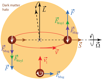
Figure 4: Spinning bodies moving in a “pseudo-isothermal” DM halo. For a body in quasi-circular orbits, with spin lying in the orbital plane, the Magnus ($\bm{F}_{{\rm Mag}}$) and Weyl ($\bm{F}_{{\rm Weyl}}$) forces are parallel. The total force is of the form $\bm{F}=A(r)\bm{S}\times\bm{v}$, pointing outwards the orbital plane on one half of the orbit, and inwards the other half; this “torques” the orbit, leading to a secular orbital precession $\bm{\Omega}$. For a body moving radially towards the center of the halo, $\bm{F}_{{\rm Weyl}}=0$, and so the total force exerted on it reduces to the Magnus force: $\bm{F}=\bm{F}_{{\rm Mag}}=4\pi\rho\bm{S}\times\bm{v}_{1}$. Generically $\bm{F}_{{\rm Weyl}}$ and $\bm{F}_{{\rm Mag}}$ have different directions. If the halo’s density was uniform, $\bm{F}_{{\rm Weyl}}=0\Rightarrow\bm{F}=\bm{F}_{{\rm Mag}}$ for all particles.

$$\rho(r)=\frac{\rho_{0}}{1+\frac{r^{2}}{r_{{\rm c}}^{2}}}\,,$$ (66)

where $r_{{\rm c}}$ is the core radius. For $r\gg r_{{\rm c}}$, the velocity of the circular orbits becomes nearly constant, whilst at the same time not diverging at $r=0$ (as is the case for the isothermal profile, $\rho(r)\propto r^{-2}$). From Eqs. (66), (57), and (61), we have

$$A(r)=12\pi\rho_{0}\frac{r_{{\rm c}}^{2}}{r^{2}}\left[1-\frac{r_{{\rm c}}}{r}\arctan\left(\frac{r}{r_{{\rm c}}}\right)\right]\,.$$ (67)

Notice that $A(r)>0$ for all $r$.

Substitution of the expressions for $\rho(r)$ and $A(r)$ in (59)-(60), (63), yield, for each model, the gravitomagnetic tidal tensor $\mathbb{H}_{ij}$ as measured by the body moving with velocity $\bm{v}$, and the spin-curvature force exerted on it. Comparing with the situation for the uniform halo highlights the contrast between the two components of the spin-curvature force (and the dependence of the Weyl force on the details of the system): $\bm{F}_{{\rm Mag}}$ remains formally the same (for it depends only on the local density $\rho$ and on $\bm{v}$), whereas $\bm{F}_{{\rm Weyl}}$ is now generically nonzero. It is different for each model, and has generically a different direction from $\bm{F}_{{\rm Mag}}$. The Weyl force vanishes remarkably when (at some instant) $\bm{v}\parallel\bm{r}$. Hence, if one takes a particle with initial radial velocity, initially one has, exactly, $\bm{F}=\bm{F}_{{\rm Mag}}$; and afterwards the spin-curvature force will consist on $\bm{F}_{{\rm Mag}}$ plus a smaller correction $\bm{F}_{{\rm Weyl}}$ due to the nonradial component of the velocity that the particle gains due to the force’s own action.

IV.3 Objects on quasi-circular orbits

We shall now consider the effect of the spin-curvature force ($\bm{F}_{{\rm Mag}}+\bm{F}_{{\rm Weyl}}$) exerted on test bodies on (quasi-) circular orbits within the DM halo. The evolution equation for the spin vector of a spinning body reads, in an orthonormal system of axes tied to the PN background frame (i.e., to the basis vectors of the coordinate system in (35); this is a frame anchored to the “distant stars”) Misner:1974qy ; CiufoliniWheeler ; Costa:2015hlh

$$\frac{d\bm{S}}{dt}=\bm{\Omega}_{{\rm s}}\times\bm{S}\ ;\qquad\ \bm{\Omega}_{{\rm s}}=-\frac{1}{2}\bm{v}\times\bm{a}+\frac{3}{2}\bm{v}\times\bm{G}\,,$$ (68)

where the first term is the Thomas precession and the second the geodetic (or de Sitter) precession. Since the only force present is the spin-curvature force, then $\bm{a}=\bm{F}/m$, and the Thomas precession is negligible to first PN order. So, in what follows, $\bm{\Omega}_{{\rm s}}\approx 3\bm{v}\times\bm{G}/2$. Without loss of generality, let us assume the orbit to lie in the $xy$-plane. Two notable cases to consider are the following.

IV.3.1 Spin orthogonal to the orbital plane ($\bm{S}=S^{z}\bm{e}_{z}$)

In this case $\bm{\Omega}_{{\rm s}}\parallel\bm{S}$, and so $d\bm{S}/dt=0$, i.e., the components of the spin vector are constant along the orbit (so it remains along $\bm{e}_{z}$). The Magnus and Weyl forces are

$$\bm{F}_{{\rm Mag}}=-4\pi\rho\frac{(\bm{S}\cdot\bm{L})}{mr}\bm{e}_{r}\,,\quad\bm{F}_{{\rm Weyl}}=\bm{F}_{{\rm Mag}}+A(r)\frac{(\bm{S}\cdot\bm{L})}{mr}\bm{e}_{r}\,,$$ (69)

where $\bm{L}=m\bm{r}\times\bm{v}$ is (to lowest order) the orbital angular momentum (see e.g. CiufoliniWheeler ). All the forces are radial. For $A(r)<4\pi\rho$, $\bm{F}_{{\rm Weyl}}$ points in the same direction of $\bm{F}_{{\rm Mag}}$, which resembles case 1 of the slab in Sec. III.2. For $A(r)>4\pi\rho$, which is the case in all the models considered in Sec. IV.2, $\bm{F}_{{\rm Weyl}}$ points in the direction opposite to $\bm{F}_{{\rm Mag}}$, resembling case 2 of the slab. As for the total force $\bm{F}$, it points in the same direction of $\bm{F}_{{\rm Mag}}$ for $A(r)<8\pi\rho$, which, for the power law profiles $\rho\propto r^{-\gamma}$ in Sec. IV.2, is the case for $\gamma<1.5$; it vanishes when $A(r)=8\pi\rho$; and it points in opposite direction to $\bm{F}_{{\rm Mag}}$ when $A(r)>8\pi\rho$, which is the case for $\gamma>1.5$. The pseudo-isothermal profile (66) realizes all the three cases, having an interior region where $\bm{F}\parallel\bm{F}_{{\rm Mag}}$, whereas $\bm{F}\parallel-\bm{F}_{{\rm Mag}}$ for large $r$. The orbital effect of $\bm{F}$ amounts to a change in the effective gravitational attraction.

IV.3.2 Spin parallel to the orbital plane ($S^{z}=0$)

In this case Eq. (68) tells us that $\bm{S}$ precesses, but remains always in the plane; since $\bm{\Omega}_{{\rm s}}$ is constant, this equation yields (taking, initially, $\bm{S}=S\bm{e}_{x}$)

$$\bm{S}=S\cos(\Omega_{{\rm s}}t)\bm{e}_{x}+S\sin(\Omega_{{\rm s}}t)\bm{e}_{y}\ .$$ (70)

To the accuracy needed for Eqs. (63), $\bm{v}\approx v(-\sin\phi\bm{e}_{x}+\cos\phi\bm{e}_{y})$, with $\phi=\omega t$, where $\omega$ is the orbital angular velocity. Therefore

$$\bm{S}\times\bm{v}=vS\cos(\phi-\Omega_{{\rm s}}t)\bm{e}_{z}=vS\cos[(\omega-\Omega_{{\rm s}})t]\bm{e}_{z}\ .$$ (71)

The Magnus, Weyl, and total forces then read

$$\bm{F}_{{\rm Mag}}=4\pi\rho Sv\cos[(\omega-\Omega_{{\rm s}})t]\bm{e}_{z}\,,$$

$$\bm{F}_{{\rm Weyl}}=[A(r)-4\pi\rho]Sv\cos[(\omega-\Omega_{{\rm s}})t]\bm{e}_{z}\,,$$

$$\bm{F}=A(r)\bm{S}\times\bm{v}=A(r)Sv\cos[(\omega-\Omega_{{\rm s}})t]\bm{e}_{z}\,.$$ (72)

All these forces are thus along the direction orthogonal to the orbital plane. The situation is inverted comparing to the case in Sec. IV.3.1 above: $\bm{F}_{{\rm Weyl}}$ points in the same direction of $\bm{F}_{{\rm Mag}}$ for $A(r)>4\pi\rho$, and in opposite direction for $A(r)<4\pi\rho$. For all the models considered in Sec. IV.2 (the pseudo-isothermal, and those of the form $\rho\propto r^{-\gamma}$, with $0\leq\gamma<3$), we have $A(r)>4\pi\rho$, cf. Eqs. (67), (65); so both $\bm{F}_{{\rm Weyl}}$ and the total force $\bm{F}$ point in the same direction as $\bm{F}_{{\rm Mag}}$ (the latter condition requiring only $A(r)>0$), see Fig. 4.

The force $\bm{F}$ causes the spinning body to oscillate (in the $\bm{e}_{z}$ direction) along the orbit, perturbing the circular motion. The coordinate acceleration orthogonal to the orbital plane is, from Eqs. (44)-(46), $\ddot{z}=F^{z}/m+G^{z}$. $G^{z}$ is the component of the gravitational field along $z$, that is acquired when the body oscillates out of the plane. Making a first order Taylor expansion about $z=0$, we have $G^{z}\simeq G_{z,z}|_{z=0}z\equiv G_{z,z}z$. The general solution, for $G_{z,z}<0$ and $G_{z,z}\neq-\Delta\omega^{2}$, is

$$z(t)=c_{1}\cos(\sqrt{-G_{z,z}}t)+c_{2}\sin(\sqrt{-G_{z,z}}t)+Z\cos(\Delta\omega t)\ ,$$ (73)

where

$$Z\equiv-\frac{S}{m}\frac{A(r)v}{G_{z,z}+\Delta\omega^{2}}=\frac{S}{m}\frac{A(r)v}{\Omega_{{\rm s}}(2\omega-\Omega_{{\rm s}})}\ ,$$ (74)

$c_{1}$ and $c_{2}$ are arbitrary integration constants, $\Delta\omega\equiv\omega-\Omega_{{\rm s}}$ and $r$ is the radius of the fiducial circular geodesic. In the second equality in (74) we noted, from Eq. (58), that $G_{z,z}=-G/r=-\omega^{2}$. Noticing, moreover, from Eqs. (56), (61), that

$$A(r)=3\omega^{2}=3\frac{v^{2}}{r^{2}}$$ (75)

and $\Omega_{{\rm s}}=3\omega^{3}r^{2}/2$, we can re-write (74) as a function of the orbital velocity ($v=\omega r$) only,

$$Z=\frac{S}{m}\frac{1}{v\left[1-\frac{3}{4}v^{2}\right]}\ .$$ (76)

The first two terms of Eq. (73) are independent of the spin-curvature force (if $\bm{F}=0$, they simply describe the $z$ oscillations of a circular orbit lying off the $xy$-plane), so $c_{1}$ and $c_{2}$ essentially set up the initial inclination of the orbit. Two natural choices of these constants stand out (analogous to those first found in Ref. Karpov:2003bn , for orbits around BHs).

Constant amplitude regime: $c_{1}=c_{2}=0$. In this case $z(t)=Z\cos(\Delta\omega t)$, yielding a “bobbing” motion of frequency $\Delta\omega$ and constant amplitude $Z$. They may be seen as an orbit which is inclined relative to the fiducial geodesic, and whose plane precesses with the frequency of the geodetic precession ($\Omega_{{\rm s}}$).

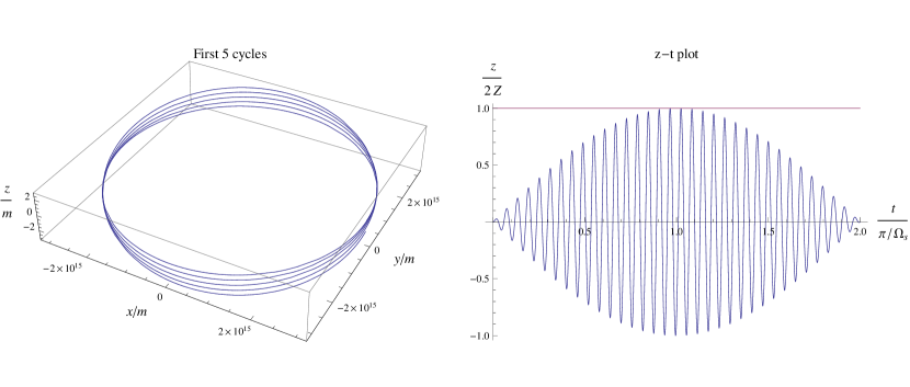
Figure 5: Numerical 1PN results for quasi-circular orbits in a pseudo-isothermal DM halo, with $\rho_{0}=10^{8}M_{\odot}{\rm pc}^{-3}$, $r_{{\rm c}}=0.02\,{\rm kpc}$ (typical of satellite galaxies Barausse:2014tra ), and $r=8r_{{\rm c}}$, case in which $v=0.15c$. The test body has the Sun’s mass $m=M_{\odot}$, and an initial spin vector $\bm{S}|_{{\rm in}}=S\bm{e}_{x}$, with $S=0.5m^{2}$. Left panel: three-dimensional plot of the orbit, showing the orbital precession $\bm{\Omega}\propto\bm{S}$ in Eq. (80) (i.e., about $\bm{e}_{x}$, initially). Right panel: plot of $z(t)/2Z$, for $t\in[0,2\pi/\Omega_{{\rm s}}]$; the numerical result agrees well with the (simplified) analytical result (77). It shows clearly the modulation by the spin precession $\bm{\Omega}_{{\rm s}}$: the orbital precession $\bm{\Omega}$ causes $z$ oscillations of initially increasing amplitude, reaching its peak $z=2Z$ at $t=\pi/\Omega_{{\rm s}}$, corresponding to the maximum inclination of the orbital plane. At that point the direction of $\bm{S}$ (thus of $\bm{\Omega}$) becomes inverted relative to the initial one, so the orbital inclination (and the oscillation amplitude) starts decreasing.

“Beating” regime: one starts with the same initial data of a circular orbit in the $xy$-plane: $z(0)=\dot{z}(0)=0$, implying $c_{2}=0$, $c_{1}=-Z$. Using the trigonometric identity $\cos(b)-\cos(a)=2\sin\left[\frac{a+b}{2}\right]\sin\left[\frac{a-b}{2}\right]$, Eq. (73) becomes

$$z(t)=2Z\sin\left[\frac{2\omega-\Omega_{{\rm s}}}{2}t\right]\sin\left[\frac{\Omega_{{\rm s}}}{2}t\right]\ .$$ (77)

This corresponds to a rapid oscillatory motion of frequency $(2\omega-\Omega_{{\rm s}})/2$ (close to the orbital frequency $\omega$), modulated by a sinusoid of frequency $\Omega_{{\rm s}}/2$ (half the frequency of the spin precession), and of peak amplitude $2Z$. In spite of the simplifying approximations made in its derivation, Eq. (77) shows very good agreement with the numerical results plotted in the right panel of Fig. 5. As shown by Eqs. (74)-(76), $Z$ is proportional to the ratio $S/m$, known as the test body’s “Møller radius” Moller1949 ; it is the minimum size an extended body can have in order to have finite spin without violating the dominant energy condition Costa:2014nta ; Moller1949 . Since $v<1$, we see from Eq. (76) that $Z$ is always larger than such radius.

The force (72) originates also a precession of the orbital plane. Recalling that (to lowest order) $\bm{L}=m\bm{r}\times\bm{v}$,

$$\frac{d\bm{L}}{dt}=m\bm{r}\times\frac{d\bm{v}}{dt}=\bm{r}\times\bm{F}=-A(r)\bm{r}\times(\bm{v}\times\bm{S})\,,$$ (78)

where we substituted $d\bm{v}/dt\equiv d^{2}\bm{x}/dt^{2}$ from Eqs. (44)-(46) (noting that $\bm{G}\times\bm{r}=0$), and $A(r)$ is given by Eq. (61). Using the vector identity $\bm{r}\times(\bm{v}\times\bm{S})=(\bm{r}\times\bm{v})\times\bm{S}+(\bm{S}\times\bm{r})\times\bm{v}$, we have

$$\frac{d\bm{L}}{dt}=A(r)\left[\frac{1}{m}\bm{S}\times\bm{L}-(\bm{S}\times\bm{r})\times\bm{v}\right]\,.$$ (79)

The first term is fixed along the orbit, and is already in a precession form. The second term must be averaged along the orbit, in order to extract the secular effect. First we note, from (68), that $\Omega_{{\rm s}}=3vG/2\sim\omega\epsilon^{2}$, so typically $\Omega_{{\rm s}}\ll\omega$, and, therefore, along one orbit, the spin vector is nearly constant. So, for averaging along an orbit, we may approximate $\bm{S}\simeq S\bm{e}_{x}$. It follows that $\left\langle(\bm{S}\times\bm{r})\times\bm{v}\right\rangle=-Srv\left\langle\sin^{2}\phi\right\rangle\bm{e}_{y}=\bm{S}\times\bm{L}/(2m)$, leading to the secular orbital precession

$$\left\langle\frac{d\bm{L}}{dt}\right\rangle=\bm{\Omega}\times\bm{L};\qquad\bm{\Omega}=\frac{A(r)}{2m}\bm{S}\ .$$ (80)

So we are led to the interesting result that the orbit precesses about the direction of the spin vector $\bm{S}$. This can be simply understood from Fig. 4: since $\bm{S}$ is nearly constant along one orbit, the force (72) points in the positive $\bm{e}_{z}$ direction for nearly half of the orbit, and in the opposite direction in the other half; this “torques” the orbit, causing it to precess. The effect is clear in the numerical results in the left panel of Fig. 5. This precession is, of course, not independent from the oscillations studied above; in fact, it is the origin of the beating regime of Eq. (77), which may be seen as follows. Multiplying the angular velocity $\Omega$ of rotation of the orbital plane by $r$, yields the “rotational velocity” of the orbit; this precisely matches [under the same assumption $\omega\gg\Omega_{{\rm s}}$ that leads to Eq. (80)] the initial slope of the function $2Z\sin(\Omega_{{\rm s}}t/2)$ that modulates (77):

$$\Omega_{{\rm s}}Z\simeq\Omega r\ .$$ (81)

So, the increase in the amplitude of the oscillations in Fig. 5 (these rapid oscillations are the variation of $z$ along each orbit, notice) is the reflex of the orbital precession $\bm{\Omega}$. Now, such orbital rotation does not go on forever in the same sense, because $\bm{S}$ itself undergoes the precession in Eq. (68), which means that after a time $t=\pi/\Omega_{{\rm s}}$ the direction of the spin vector is reversed. Likewise $\bm{\Omega}$ and $\langle d\bm{L}/dt\rangle$ are reversed (before one full revolution about $\bm{S}$ is completed if $\Omega<\Omega_{{\rm s}}$, as is usually the case), and this is why the amplitude in Eq. (77) is modulated by the geodetic spin precession $\Omega_{{\rm s}}$.

In Fig. 5 numerical results are plotted for a test body with the Sun’s mass $m=M_{\odot}$ and $S=0.5m^{2}$, in a pseudo-isothermal DM halo typical of a satellite galaxy (corresponding to much larger DM densities than those typical of the Milky Way, which makes them more suitable to illustrate the effects described above). Such results are obtained by numerically solving the system of equations formed by $md^{2}\bm{x}/dt^{2}=m\bm{G}+\bm{F}+\bm{F}_{{\rm D}}$ together with Eq. (68), with $\bm{F}$ as given by Eqs. (62)-(63), (59), (67), and $\bm{G}$ given by Eqs. (56), (57), (67). The term $\bm{F}_{{\rm D}}$ is the dynamical friction force

$$\bm{F}_{{\rm D}}=-40\pi\rho m^{2}\left({\rm erf}(X)-\frac{2X}{\sqrt{\pi}}e^{-X^{2}}\right)\frac{\bm{v}}{v^{3}}\,,\quad X=\frac{v}{v_{{\rm circ}}}\,,$$ (82)

which is here included. It follows from Eq. (8.6) of BinneyTremaine , or Eq. (3) of Pani:2015qhr , by taking $\lambda=10$ and $\sqrt{2}\sigma=v_{{\rm circ}}\equiv$ velocity of the circular orbit at $r$, cf. BinneyTremaine . (The impact of $\bm{F}_{{\rm D}}$, in the case of the motion in Fig. 5, turns out to be unnoticeable.)

IV.3.3 Particular examples in the Milky Way DM Halo

Pseudo-isothermal profile.—The DM density at the solar system position is about $0.01M_{\odot}/{\rm pc}^{3}=10^{-21}{\rm kg\,m}^{-3}$ Read:2014qva ; Gilmore:1996pr ; the Sun’s distance from the center of the Milky Way is $r_{\odot}=8\,{\rm kpc}$. The core radius $r_{{\rm c}}$ of the Milky Way DM halo is about $1\,{\rm kpc}$. Assuming the pseudo-isothermal density profile in Eq. (66), this means that $\rho_{0}=0.7M_{\odot}{\rm pc}^{-3}$. The velocity $v$ of the quasi-circular orbits is obtained from Eqs. (67), (75). For a body orbiting at $r=r_{\odot}$, the peak amplitude in Eqs. (76)-(77) then reads

$$2Z=3.5\times 10^{3}\frac{S}{m}\ .$$ (83)

The time to reach it (“beating” half period) is however very long: $t_{{\rm peak}}\approx\pi/\Omega_{{\rm s}}=10^{14}\,{\rm yr}$ ($10^{4}\times$ age of the universe); this corresponds to $\omega/(2\Omega_{{\rm s}})=10^{6}$ laps around the center. Noting that the initial of slope of the function $2Z\sin(\Omega_{{\rm s}}t/2)$ that modulates Eq. (77) is $Z\Omega_{{\rm s}}$, the maximum amplitude actually reached within the age of the universe ($\equiv t_{0}$) is

$$2Z_{{\rm today}}\equiv 2Z\sin\left[\frac{\Omega_{{\rm s}}t_{0}}{2}\right]\approx Z\Omega_{{\rm s}}t_{0}$$ (84)

$$\ \approx\Omega rt_{0}=\frac{3v^{2}t_{0}}{2r}\frac{S}{m}$$ (85)

where in the second approximate equality we used (81), and in the last equality we used (80), (75). Hence, for the setting above,

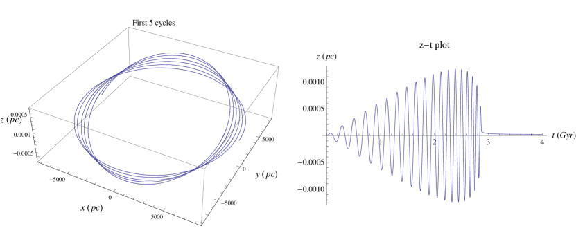
Figure 6: Orbits of a satellite galaxy in the Milky way DM halo (numerical 1PN results). Due to their disk-like shape, galaxies have a large Møller radius $S/m$, making them especially suitable test bodies for the effects under study. The satellite is assumed to be a scale reduced version of the Milky Way, of diameter 2.5${\rm kpc}$, and orbiting at a distance 8${\rm kpc}$ (= Sun’s distance) from the Halo’s center. The peak amplitude predicted by Eqs. (74)-(77) is $2Z\approx 60\,{\rm pc}$; but it is never reached, due to the very strong dynamical friction. Still a peak of about $10^{-3}\,{\rm pc}$ is reached after about $2.2\,{\rm Gyr}$ ($\simeq 1/5$ the age of the universe).

$$2Z_{{\rm today}}=1.4\times 10^{-4}Z=0.25\frac{S}{m}\ .$$ (86)

Both $Z$ and the angular velocity $\Omega$ of orbital precession, Eq. (80), are proportional to the body’s Møller radius $S/m$. For a Sun-like star ($m=M_{\odot}$, $S\approx 0.2m^{2}$ KommetAl , $S/m=3\times 10^{2}\,{\rm m}$), the effect is very small: the secular orbital precession (80) inclines the orbit by about $1.6\,{\rm m}$ per lap, with peak amplitude $2Z=10^{6}\,{\rm m}$ (about 1400 times smaller that the Sun’s diameter), and $2Z_{{\rm today}}\sim 10^{2}\,{\rm m}$. Larger or more massive bodies will typically have a larger Møller radius, thereby yielding more interesting numbers; but, on the other hand, for large $m$, the dynamical friction force $\bm{F}_{{\rm D}}$, Eq. (82) (which is proportional to $m^{2}$), becomes also important. From the known objects moving in the Milky Way’s DM halo, those with largest Møller radius are (due to their size and flattened shape) Milky Way’s satellite galaxies. Consider first, for a comparison (still at $r\simeq r_{\odot}$), a hypothetical satellite galaxy with diameter $\simeq 2.5\,{\rm kpc}$, and assume it to be a “scale reduced” version of the Milky Way (diameter $55\,{\rm kpc}$, mass $m_{{\rm MW}}=10^{12}M_{\odot}$, angular momentum $S_{{\rm MW}}=2.6\times 10^{31}\,{\rm m}^{2}$), rotating with the same velocity. Since $S\propto mv_{{\rm rot}}R$, this yields $S_{{\rm sat}}/S_{{\rm MW}}\sim(2.5/55)^{4}$, $m_{{\rm sat}}/m_{{\rm MW}}\sim(2.5/55)^{3}$, leading to a Møller radius $S_{{\rm sat}}/m_{{\rm sat}}\sim 0.02\,{\rm pc}$. In this case the orbit inclines at an initial rate of $4\times 10^{12}\,{\rm m}$ per orbit ($2\times 10^{4}\,{\rm m}$ per year), and the peak amplitude, as predicted by Eqs. (74)-(77), (83) would now be $2Z\simeq 60{\rm pc}$. Such large peak value however is never reached, due to the damping action of $\bm{F}_{{\rm D}}$; the numerical results shown in Fig. 6 show that a peak of about $0.001\,{\rm pc}$ (i.e., about 10 times the radius of the solar system), is reached within about $2.2{\rm Gyr}$ (a fifth of the age of the universe), after which the orbit and its oscillations pronouncedly decay. As a concrete example in the Milky Way DM Halo, we take the Large Magellanic Cloud (the largest satellite galaxy), located at $r=48\,{\rm kpc}$ from the MW center. It has mass $m_{{\rm LMC}}\approx 10^{10}M_{\odot}$, diameter $\approx 4.3\,{\rm kpc}$, and rotational velocity $v_{{\rm rot}}\approx 9\times 10^{4}\,{\rm m\,s^{-1}}$ vanderMarel:2013jza , from which we estimate a Møller radius $S_{{\rm LMC}}/m_{{\rm LMC}}\sim 0.3\,{\rm pc}$. We find a gradual inclination of the orbit of about $\sim 4\times 10^{-9}\,{\rm mas}{\rm yr}^{-1}$ (or $3\times 10^{4}\,{\rm m}\,{\rm yr}^{-1}$); this is far beyond the current observational accuracy, since the uncertainty in the LMC’s proper motion is presently much larger ($\sim 10^{-2}{\rm mas}{\rm yr}^{-1}$ vanderMarel:2013jza ). The peak amplitude predicted by Eqs. (74)-(77), (83) is $2Z\approx 1\,{\rm kpc}$ (which, again, is not reached due to dynamical friction). Numerical simulations (similar to those in Fig. 6) show that an effective peak of about $10^{-3}\,{\rm pc}$ is reached within $2.5\,{\rm Gyr}$.

Power law profiles.— For the models of the form $\rho(r)=Kr^{-\gamma}$ in Sec. IV.2, substituting (65) in (75), (80), it follows from Eqs. (76) and (85) that

$$2Z\approx\frac{2S}{mv}=\frac{S}{m}\left[\frac{3-\gamma}{K\pi}\right]^{1/2}r^{\gamma/2-1}\ ,$$ (87)

$$2Z_{{\rm today}}\approx\Omega rt_{0}=\frac{S}{m}\frac{6\pi t_{0}K}{3-\gamma}r^{1-\gamma}\ ,$$ (88)

where $K$ is determined from the value of $\rho(r_{\odot})$ which we assume, for all models, $\rho(r_{\odot})\approx 0.01M_{\odot}{\rm pc}^{-3}$ Bertone:2005hw ; Read:2014qva ; Gilmore:1996pr . For $\gamma=1$, $Z_{{\rm today}}\approx 0.08S/m$ is approximately constant, and $Z$ decreases with $r$ as $Z\propto r^{-1/2}$; for bodies orbiting at $r=r_{\odot}$, one has $Z\approx 2.3\times 10^{3}S/m$. That is, the peak/present time amplitudes are, respectively (at $r=r_{\odot}$), somewhat larger/smaller than those for the pseudo-isothermal profile, Eqs. (83), (86). For $1<\gamma<2$, it follows from Eqs. (88) that both $Z$ and $Z_{{\rm today}}$ decrease with $r$. The isothermal case, $\gamma=2$, yields a $Z=1.6\times 10^{3}S/m$ approximately independent of $r$, and $Z_{{\rm today}}\propto r^{-1}$. At $r=r_{\odot}$, $Z_{{\rm today}}=0.15S/m$; thus $Z$ is slightly smaller and $Z_{{\rm today}}$ slightly larger that in the pseudo-isothermal profile. However, contrary to the pseudo-isothermal case (where $Z_{{\rm today}}$ reaches a maximum $\approx 0.26S/m$ at $r\approx 1.5{\rm kpc}$), $Z_{{\rm today}}$ increases steeply as one approaches the halo center, approaching the peak value $Z$ [cf. Eq. (85)].

Inside the galactic disk.—The above are results taking into account DM only; so they apply to orbits outside the galactic disk. Within the disk, the density of baryonic matter, in the vicinity of the Sun, is about $\rho_{{\rm b}}\approx 0.1M_{\odot}{\rm pc}^{-3}$ BinneyTremaine ; Read:2014qva , i.e. one order of magnitude larger than that of DM. This leads to an enlarged effect. The field produced by the disk is a complicated problem (see Sec. V below). The analysis of a simple model in Sec. V.2 reveals however that, just for an order of magnitude estimate, the force caused by the disk can be taken as the corresponding Magnus force $\bm{F}_{{\rm Mag}}$, and its contribution to the orbital precession as $\Omega_{{\rm b}}\sim F_{{\rm Mag}}/(vm)\sim 4\pi\rho_{{\rm b}}S/m$. Assuming, for DM, the pseudo-isothermal profile (66), leads to $2Z_{{\rm today}}\approx\Omega rt_{0}\sim 2S/m$, cf. Eq. (85) [here $\Omega\equiv\Omega_{{\rm b}}+\Omega_{{\rm DM}}$, with $\Omega_{{\rm DM}}$ given by Eqs. (80), (67)].

More importantly, the galactic disk might reveal a signature of the orbital precession (80): BHs or stars with spin axes nearly parallel to the galactic plane are, on average, more distant from the plane than other bodies, by a distance of order $\sim 4Z_{{\rm today}}/\pi$. This effect might be observable. The most precise map of the sky is expected to be given by the Gaia mission Gaia , able to measure angles of about $2\times 10^{-11}$ rads. Therefore, on test bodies whose distance $d$ from Gaia (i.e., from the Earth) is such that $d\lesssim 4Z_{{\rm today}}/(\pi 2\times 10^{-11})$, the effect would be within the angular resolution. To be concrete, consider a giant star like Antares; it has radius $R_{{\rm ant}}\sim 10^{3}R_{\odot}$, mass $m_{{\rm ant}}\sim 12M_{{\rm\odot}}$, surface rotational velocity $v_{{\rm rot}}=7\times 10^{-5}$. For simplicity, assume it to be uniform and rotate rigidly, leading to a Møller radius $S_{{\rm ant}}/m_{{\rm ant}}=2\times 10^{7}\,{\rm m}$ (five orders of magnitude larger than that of the Sun). Assuming the pseudo-isothermal profile, this yields a present time amplitude $2Z_{{\rm today}}\sim 2S/m=4\times 10^{7}\,{\rm m}$. Giants of this type, with spin axes nearly parallel to the galactic plane, should on average be farther from the plane than others, by about $\sim 3\times 10^{7}\,{\rm m}$ ($\sim 10^{-5}\times$ Antares’s diameter). Considering the density value at $r=r_{\odot}$, their maximum allowed distance from the Earth (so that the effect can be detected) is then $d_{{\rm max}}\approx 0.04\,{\rm kpc}$, which is not far from the order of magnitude of Antares’ actual distance ($d=0.17\,{\rm kpc}$), and of other large stars. Thus, albeit small, the effect on such stars is close to the angular resolution. The matter density (baryonic and DM) increases however as one approaches the galaxy center; for stars along the line connecting the solar system to the center, the angle that the effect subtends on the GAIA spacecraft is $\theta\approx Z_{{\rm today}}/d$, with $d=r_{\odot}-r$. For DM models of the type $\rho_{{\rm DM}}\propto r^{-\gamma}$ with $\gamma>1$, the angle $\theta$ increases with decreasing $r$ (after initially decreasing, and bouncing), cf. Eq. (88). Considering the isothermal profile ($\gamma=2$), and taking into account DM only, $\theta$ enters GAIA’s resolution for $r\lesssim 4{\rm pc}$. The Magnus signature on the galactic disk might thus serve as a test for such models. Independently of such DM models, the baryonic matter is known to reach high densities in the galaxy’s inner regions; using $\rho_{{\rm b}}(r)$ as given in Eq. (2) of Genzel2003 , we have that, for $r\lesssim 1{\rm pc}$, the baryonic matter alone is sufficient for $\theta$ to enter GAIA’s resolution.

V Magnus effect in accretion disks

The gravitational Magnus effect due to DM is limited by its typically very low density. Accretion disks around BHs or stars provide mediums with relatively much higher densities, where the effect can be more significant, possibly within the reach of near future observational accuracy.

V.1 Orders of magnitude for a realistic density profile

The standard model for relativistic thin disks is the Novikov-Thorne model NovikovThorne1973 , which generalizes the Shakura-Sunyaev Shakura:1972te model to include relativistic corrections. According to such model the disk is divided into different regions, the outer and more extensive of them being well approximated by the Newtonian counterpart. The density of the later reads (in the equatorial plane) Shakura:1972te

$$\rho=\frac{f_{{\rm Edd}}^{11/20}}{\tilde{r}^{15/8}}\alpha^{-7/10}\left[\frac{M_{\odot}}{M_{{\rm BH}}}\right]^{\frac{7}{10}}\left[1-\sqrt{\frac{6}{\tilde{r}}}\right]^{\frac{11}{20}}1\times 10^{6}{\rm kg}\,{\rm m}^{-3}\,,$$ (89)

where $\tilde{r}\equiv r/M_{{\rm BH}}$, $M_{{\rm BH}}$ is the mass of the central BH, $\tilde{r}_{{\rm in}}\equiv r_{{\rm in}}/M_{{\rm BH}}$, $\alpha$ the “viscosity parameter” and $f_{{\rm Edd}}$ Eddington’s ratio for mass accretion (e.g. Barausse:2014tra ). The density (89) leads to a Magnus force $\bm{F}_{{\rm Mag}}=4\pi\rho\bm{S}\times\bm{v}$ (cf. Eq. (41)) of interesting magnitude, compared with other relevant forces.

Comparing with the Newtonian gravitational force $m\bm{G}_{{\rm BH}}$ exerted on the body by the central BH, we have $F_{{\rm Mag}}/(m\|\bm{G}_{{\rm BH}}\|)\sim r^{2}\rho vS/(mM_{{\rm BH}})$. Different estimates can be made. Let us consider the case of a binary of BHs with similar masses $m\sim M_{{\rm BH}}$; in this case $F_{{\rm Mag}}/(m\|\bm{G}_{{\rm BH}}\|)\sim\tilde{S}r^{2}\rho v$, where $\tilde{S}\equiv S/m^{2}$ (for a fast spinning BH $\tilde{S}\lesssim 1$; for extended bodies it could be much larger). Now we need an estimate for $v$ (the velocity of the “test” body with respect to the disk of the “source” BH); it can be taken has having the magnitude $v\sim\sqrt{M_{{\rm BH}}/r}=\tilde{r}^{-1/2}$ . Then [converting ${\rm kg}\,{\rm m}^{-3}$ to geometrized units, and using $M_{{\rm BH}}=M_{\odot}(M_{{\rm BH}}/M_{\odot})$],

$$\frac{F_{{\rm Mag}}}{m\|\bm{G}_{{\rm BH}}\|}\sim\tilde{S}\mathcal{F}(M_{{\rm BH}})\left[1-\sqrt{\frac{6}{\tilde{r}}}\right]^{\frac{11}{20}}\tilde{r}^{-3/8}\$$ (90)

where

$$\mathcal{F}(M_{{\rm BH}})\equiv 1.6\times 10^{-15}f_{{\rm Edd}}^{11/20}\alpha^{-7/10}\left[\frac{M_{{\rm BH}}}{M_{\odot}}\right]^{\frac{13}{10}}\ .$$

Let us now compare the magnitude of $\bm{F}_{{\rm Mag}}$ with the spin-orbit force $\bm{F}_{{\rm SO}}$ exerted on the “test” body due to its spin $\bm{S}$ (given by Eq. (97) below). Assume it to move, relative to the central BH, with velocity $\sim v$ (i.e, of the same order of magnitude of that relative to the matter in the disk, see footnote 14) so that $\bm{F}_{{\rm SO}}\sim M_{{\rm BH}}vS/r^{3}$. It follows that

$$\frac{F_{{\rm Mag}}}{F_{{\rm SO}}}\sim\frac{\rho r^{3}}{M_{{\rm BH}}}=\mathcal{F}(M_{{\rm BH}})\left[1-\sqrt{\frac{6}{\tilde{r}}}\right]^{\frac{11}{20}}\tilde{r}^{9/8}\ .$$ (91)

Comparing with the magnitude of the spin-spin force $F_{{\rm SS}}\sim S_{{\rm BH}}S/r^{4}$ Wald:1972sz ,

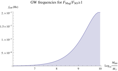
Figure 7: Range of frequencies of the emitted gravitational radiation for binary systems in which the Magnus force $F_{{\rm Mag}}$ is larger than $F_{{\rm SO}}$ and $F_{{\rm SS}}$, for $\alpha=0.01$, $f_{{\rm Edd}}=0.2$ [see Eq. (89)] and $S_{{\rm BH}}=0.1M_{{\rm BH}}^{2}$. The solid curves represent, as functions of the central BH’s mass ($M_{{\rm BH}}$), the frequencies for which $F_{{\rm Mag}}\sim F_{{\rm SO}}$ and $F_{{\rm Mag}}\sim F_{{\rm SS}}$. In the shadowed regions it holds, respectively, $F_{{\rm Mag}}\gtrsim F_{{\rm SO}}$ and $F_{{\rm Mag}}\gtrsim F_{{\rm SS}}$. The Magnus force tends to be the leading spin dependent force at low frequencies and for SMBHs, namely within the band of pulsar timing arrays ($10^{-9}{\rm Hz}\lesssim f_{{\rm GW}}\lesssim 10^{-7}{\rm Hz}$). The frequency for which $F_{{\rm Mag}}\sim F_{{\rm SS}}$ lies moreover just below (or within, depending on $\alpha$, $f_{{\rm Edd}}$, and $S_{{\rm BH}}$) the LISA band.

$$\frac{F_{{\rm Mag}}}{F_{{\rm SS}}}\sim\frac{\rho vr^{4}}{S_{{\rm BH}}}=\frac{\rho vr^{4}}{\tilde{S}_{{\rm BH}}M_{{\rm BH}}^{2}}=\frac{\mathcal{F}(M_{{\rm BH}})}{\tilde{S}_{{\rm BH}}}\left[1-\sqrt{\frac{6}{\tilde{r}}}\right]^{\frac{11}{20}}\tilde{r}^{13/8}\ ,$$ (92)

where $\tilde{S}_{{\rm BH}}\equiv S_{{\rm BH}}/M_{{\rm BH}}^{2}$.

Finally, let us compare the magnitude of $\bm{F}_{{\rm Mag}}$ with that of the “orbit-orbit” gravitomagnetic forces $\bm{F}_{{\rm OO}}=\bm{v}_{1}\times\bm{H}_{1{\rm trans}}$ in the binary; that is, the force exerted on the “test” body (dub it body 2) due to the gravitomagnetic field $\bm{H}_{1{\rm trans}}$ generated by the translational motion of the “source” (body 1), with respect to the binary center of mass frame. This is of interest in this context for being an effect that has already been detected to very high accuracy in binaries (relative uncertainty of about $10^{-3}$, in observations of the Hulse-Taylor pulsar Nordtvedt:1988vt ). It is moreover typically larger than its spin-spin and spin-orbit counterparts. The translational gravitomagnetic field is given by Eq. (119) ($\bm{H}_{1}=\bm{H}_{1{\rm trans}}$ therein); so $F_{{\rm OO}}\sim mM_{{\rm BH}}v_{1}v_{2}/r^{2}$, which we may take as $F_{{\rm OO}}\sim mM_{{\rm BH}}v^{2}/r^{2}$ (see footnote 14). Considering moreover $m\sim M_{{\rm BH}}$, we have

$$\frac{F_{{\rm Mag}}}{F_{{\rm OO}}}\sim\frac{\rho\tilde{S}r^{2}}{v}=\tilde{S}\mathcal{F}(M_{{\rm BH}})\left[1-\sqrt{\frac{6}{\tilde{r}}}\right]^{\frac{11}{20}}\tilde{r}^{5/8}\ ,$$ (93)

where, again, we used $v\sim\sqrt{M_{{\rm BH}}/r}$.

All the four ratios (90)-(93) increase with $M_{{\rm BH}}$, and depend also on $r$; the ratio to the Newtonian force decreases with $r$, whereas all the others increase with $r$. Choosing, from the range of values in Barausse:2014tra , $\alpha\sim 0.01$, $f_{{\rm Edd}}\sim 0.2$, and considering supermassive BHs with $M_{{\rm BH}}\sim 10^{9}M_{\odot}$, $F_{{\rm Mag}}$ starts being larger than $F_{{\rm SO}}$ for $r\gtrsim 81M_{{\rm BH}}$. Assuming the central black hole to be fast spinning (unfavorable case) with e.g. $\tilde{S}_{{\rm BH}}\sim 0.1$, we have that $F_{{\rm Mag}}\gtrsim F_{{\rm SS}}$ for $r\gtrsim 17M_{{\rm BH}}$. Assuming moreover that the “test” black hole is also fast spinning (favorable scenario) with e.g. $\tilde{S}=0.5$, $F_{{\rm Mag}}\gtrsim F_{{\rm OO}}$ for $r\gtrsim 6\times 10^{3}M_{{\rm BH}}$. Even comparing with the Newtonian force, the magnitude of $F_{{\rm Mag}}$ is interesting: for $r\lesssim 2\times 10^{4}M_{{\rm BH}}$, we have $F_{{\rm Mag}}/(m\|\bm{G}\|)\gtrsim 10^{-4}$; this is the same order of magnitude of the leading 1PN corrections (which are of fractional order $\epsilon^{2}\sim M_{{\rm BH}}/r\sim 10^{-4}$, see Sec. III.1).

These comparisons are relevant for binary systems, due to the impact of spin effects (both spin-orbit and spin-spin) in the emitted gravitational radiation, which is expected to be observed in the near future Hannam:2013pra ; LangHughes2006 ; Vecchio:2003tn ; Lang:2007ge ; Stavridis:2009ys ; Schmidt:2014iyl ; Berti:2004bd . There are different existing/proposed detectors, operating at different frequencies (see e.g. Moore:2014lga ). The frequency $f_{{\rm GW}}$ of the emitted gravitational radiation is approximately related to the Kepler orbital angular velocity $\omega$ by $f_{{\rm GW}}=\omega/\pi$. Since $\omega\approx M_{{\rm BH}}^{1/2}r^{-3/2}=M_{{\rm BH}}^{-1}\tilde{r}^{-3/2}$, one may eliminate either $M_{{\rm BH}}$ or $\tilde{r}$ from Eqs. (89)-(93) above. Eliminating $\tilde{r}$ [by substituting $\tilde{r}\rightarrow(\omega M_{{\rm BH}})^{-2/3}$] one obtains $\rho(M_{{\rm BH}},\omega)$, and all the ratios above, as functions of $M_{{\rm BH}}$ and $\omega$. We are especially interested in the ratios to the spin-spin and spin-orbit forces; they both decrease with $\omega$; hence, solving for $\omega$ the equalities $F_{{\rm Mag}}/F_{{\rm SO}}=1$ and $F_{{\rm Mag}}/F_{{\rm SS}}=1$ yields, as a function of $M_{{\rm BH}}$, the maximum orbital angular velocity $\omega_{{\rm max}}(M_{{\rm BH}})$ [and thus the maximum gravitational wave frequency $f_{{\rm GWmax}}(M_{{\rm BH}})$] allowed in order to have $F_{{\rm Mag}}$ larger than $F_{{\rm SS}}$ or $F_{{\rm SO}}$. These curves are plotted in Fig. 7, for $\alpha\sim 0.01$, $f_{{\rm Edd}}\sim 0.2$, and $\tilde{S}_{{\rm BH}}=0.1$. They tell us that the Magnus force is more important at low frequencies, and for supermassive black holes. Within the band of groundbased detectors such as LIGO ($10{\rm Hz}\lesssim f_{{\rm GW}}\lesssim 10^{3}{\rm Hz}$) it is much smaller than $F_{{\rm SO}}$ and $F_{{\rm SS}}$. Within the band of the spacebased LISA Audley:2017drz ($10^{-5}{\rm Hz}\lesssim f_{{\rm GW}}\lesssim 1{\rm Hz}$), we have that $F_{{\rm Mag}}\ll F_{{\rm SO}}$. Fixing the frequency at the most favorable value $f_{{\rm GW}}=10^{-5}{\rm Hz}$ (i.e., fixing $\omega\sim 3\times 10^{-5}{\rm s^{-1}}$), and plotting the corresponding ratio $F_{{\rm Mag}}/F_{{\rm SO}}=\rho(M_{{\rm BH}})/\omega^{2}$ (not shown in Fig. 7), one sees that $F_{{\rm Mag}}/F_{{\rm SO}}\lesssim 10^{-2}$. On the other hand, Fig. 7 shows also that the frequency for which $F_{{\rm Mag}}\sim F_{{\rm SS}}$ lies just below the LISA band. In fact, the magnitude of $F_{{\rm Mag}}$ is already comparable to $F_{{\rm SS}}$ within LISA’s band (for $f_{{\rm GW}}\sim 10^{5}{\rm Hz}$, $F_{{\rm Mag}}$ reaches a maximum $F_{{\rm Mag}}\sim 0.2F_{{\rm SS}}$ for $M\sim 10^{7.5}M_{\odot}$). Moreover, mild deviations in the disk parameters from the conservative choice above (e.g., $\alpha\sim 0.005$, $f_{{\rm Edd}}\sim 0.8$ Shakura:1972te ), or simply considering a central black hole with smaller spin (e.g. $\tilde{S}_{{\rm BH}}\sim 0.03$) are sufficient to make $F_{{\rm Mag}}$ of the same order of magnitude as $F_{{\rm SS}}$ within such band. Since LISA is expected to be sensitive to spin-spin effects LangHughes2006 ; Berti:2004bd , this suggests that there might be prospects of detecting as well the Magnus effect. The lowest frequency planned detectors are pulsar timing arrays (PTAs, see e.g. Hobbs2009 ; Detweiler1979 ; Sazhin ; Moore:2014eua ; Moore:2014lga ; Arzoumanian2016 ), of band $10^{-9}{\rm Hz}\lesssim f_{{\rm GW}}\lesssim 10^{-7}{\rm Hz}$, and which in the future are expected to detect waves from individual SMBH binary sources Hobbs2009 ; Moore:2014eua . Within this band, Fig. 7 shows that $F_{{\rm Mag}}$ can be the leading spin effect.

V.2 Miyamoto-Nagai disks

Although to compute the Magnus force (41) all one needs to know is the disk’s local density $\rho$ and the relative velocity $\bm{v}$ of the test body, in order to determine the body’s motion, one needs the total spin-curvature force $\bm{F}=\bm{F}_{{\rm Mag}}+\bm{F}_{{\rm Weyl}}$; that requires knowledge of the gravitational field produced by the sources (disk plus central BH), since $\bm{F}_{{\rm Weyl}}$ depends on it. This is however a complicated problem. There is an extensive literature on the fields of disks, from exact solutions Semerak:2012dw ; Morgan:1969jr ; Lemos:1988vf ; Lemos:1993uy ; Bicak:1993xat ; Espitia:2001cj ; Bicak:1993zz ; NishidaEriguchiLanza ), to perturbative Cizek:2017wzr ; Kotlarik:2018nbd , PN Jaranowski:2014yva , and Newtonian Miyamoto:1975zz ; Baes:2008td ; Vogt:2009sy ; Witzany:2015yqa solutions. Even though the formalism in Sec. III (by being exact) could in principle be used to treat the exact problem, most exact solutions in the literature are not practical or suitable for our problem, since they are either nonanalytical NishidaEriguchiLanza ; Kotlarik:2018nbd , or describe the field only outside the disk Semerak:2012dw , or are not realistic models of astrophysical systems Semerak:2012dw ; Bicak:1993zz ; Morgan:1969jr ; Lemos:1988vf ; Lemos:1993uy ; Bicak:1993xat ; Espitia:2001cj . In this context the Newtonian solutions provide the more treatable examples for us. According to Eq. (43), to compute $\bm{F}_{{\rm Weyl}}$ (and thus $\bm{F}$) to leading PN order, only the Newtonian and gravitomagnetic ($\bm{H}$) fields of the source are needed. By considering a Newtonian field, one is ignoring the gravitomagnetic fields (frame-dragging) produced by the rotation of the disk (and of the central BH); this would be accurate if either the disk was static, or composed of counterrotating streams of matter, or the test body moves considerably faster relative to the disk than the disk’s average rotational velocity (so that one can have $vG\gg H$). One might argue that none of these is a realistic assumption — the disk is (at least in part) gravitationally driven, so it must rotate, with a velocity of the same order of magnitude of the velocity of orbiting test bodies. But still it is no less realistic than most exact solutions — which are precisely static Semerak:2012dw ; Morgan:1969jr ; Lemos:1988vf ; Lemos:1993uy ; Bicak:1993xat ; Espitia:2001cj and/or composed of streams of matter flowing in opposite directions Morgan:1969jr ; Lemos:1988vf ; Lemos:1993uy ; Bicak:1993xat ; Espitia:2001cj ; Bicak:1993zz . More realistic solutions, where $\bm{H}$ is taken into account, are found in PN theory; the field is however very complicated already at 1PN, and not obtained analytically (e.g. Jaranowski:2014yva ). So, here, just to illustrate the basic features of the spin-curvature force produced by the disk, we consider one of the simplest Newtonian 3D models, the Miyamoto-Nagai disks Miyamoto:1975zz ; Baes:2008td ; Vogt:2009sy , also called the “inflated” Kusmin model Vogt:2009sy . The Newtonian potential is

$$U(\varrho,z)=\frac{M_{{\rm disk}}}{\sqrt{\varrho^{2}+(\sqrt{z^{2}+b^{2}}+a)^{2}}}+\frac{M_{{\rm BH}}}{r}\equiv U_{{\rm disk}}+U_{{\rm BH}}$$ (94)

where $\varrho^{2}=x^{2}+y^{2}$, $M_{{\rm disk}}$ is the disk’s total mass, and $b$ and $a$ are constants with dimensions of length. The ratio $b/a$ is a measure of the flatness of the disk Miyamoto:1975zz . The Laplace equation $\nabla^{2}U=\nabla^{2}U_{{\rm disk}}=-4\pi\rho$ yields the disk’s density, Eq. (5) of Miyamoto:1975zz . The Weyl force is obtained from Eq. (43), which reads here $F_{{\rm Weyl}}^{i}=2\epsilon_{\ km}^{(i}G^{j),m}v^{k}S_{j}$, where $\bm{G}$ is, to the accuracy needed for this expression, the sum of the Newtonian fields produced by the disk and the central BH, $\bm{G}\simeq\nabla U_{{\rm disk}}+\nabla U_{{\rm BH}}$. It can be split into the Weyl forces due to the disk and due to the central BH, which read explicitly, in the equatorial plane

$$\bm{F}_{{\rm Weyl}}=\bm{F}_{{\rm Weyldisk}}+\bm{F}_{{\rm BH}}$$ (95)

$$F_{{\rm Weyldisk}}^{j}=\ \frac{M_{{\rm disk}}}{\left[r^{2}+(a+b)^{2}\right]^{\frac{3}{2}}}\left[(\bm{S}\times\bm{v})^{j}|_{j\neq z}-\epsilon_{\ ik}^{j}S^{i}v^{k}|_{i\neq z}\right.$$

$$\left.-\frac{3r^{j}(\bm{S}\times\bm{v})\cdot\bm{r}+3(\bm{r}\cdot\bm{S})(\bm{v}\times\bm{r})^{j}}{r^{2}+\left(a+b\right)^{2}}\right]$$

$$+\frac{(a+b)M_{{\rm disk}}}{b\left[r^{2}+(a+b)^{2}\right]^{\frac{3}{2}}}\left[\delta_{z}^{j}(\bm{S}\times\bm{v})^{z}+S^{z}\epsilon^{jkz}v_{k}\right]$$ (96)

$$\bm{F}_{{\rm BH}}=-\frac{3M_{{\rm BH}}}{r^{3}}\left[\bm{v}\times\bm{S}+\frac{2\bm{r}[(\bm{v}\times\bm{r})\cdot\bm{S}]}{r^{2}}+\frac{(\bm{v}\cdot\bm{r})\bm{S}\times\bm{r}}{r^{2}}\right]$$ (97)

(Notice that $\bm{F}_{{\rm BH}}$ is the well-known expression for the spin-orbit part of the spin-curvature force exerted by a BH on a spinning body, e.g. Eq. (44) of Wald:1972sz ).

Quasi-circular orbits

We shall now consider the effect of the spin-curvature force ($\bm{F}_{{\rm Mag}}+\bm{F}_{{\rm Weyl}}$) produced by the disk on test bodies on (quasi-) equatorial circular orbits around the central object. This demands the central object to be much more massive than the test body, $M_{{\rm BH}}\gg m$. We also consider the test body to be a BH, in order to preclude surface effects (such as an ordinary Magnus effect), and ensure that the motion is gravitationally driven. In the equatorial plane $\varrho=r$, thus the disk’s density $\rho=-\nabla^{2}U/4\pi$, that follows from (94), is

$$\rho=\frac{M_{{\rm disk}}}{4\pi\left[r^{2}+\left(a+b\right)^{2}\right]^{3/2}}\left[3-\frac{3r^{2}}{r^{2}+\left(a+b\right)^{2}}+\frac{a}{b}\right]$$ (98)

(cf. Eq. (5) of Miyamoto:1975zz ). As in Sec. IV.2, there are two notable cases to consider.

Spin parallel to the symmetry axis ($\bm{S}=S^{z}\bm{e}_{z}$). Equation (68) tells us that, in this case, the components of $\bm{S}$ are constant. The Magnus, Weyl and total force due to the disk, $\bm{F}_{{\rm disk}}\equiv\bm{F}_{{\rm Mag}}+\bm{F}_{{\rm Weyldisk}}$, are

$$\bm{F}_{{\rm Mag}} =-4\pi\rho\frac{(\bm{S}\cdot\bm{L})}{mr}\bm{e}_{r}\,,$$

$$\bm{F}_{{\rm Weyldisk}} =\frac{(\bm{S}\cdot\bm{L})M_{{\rm disk}}}{mr\left[r^{2}+\left(a+b\right)^{2}\right]^{3/2}}\left[\frac{3r^{2}}{r^{2}+\left(a+b\right)^{2}}+\frac{a}{b}\right]\bm{e}_{r},$$

$$\bm{F}_{{\rm disk}} =\frac{3(\bm{S}\cdot\bm{L})M_{{\rm disk}}}{mr\left[r^{2}+\left(a+b\right)^{2}\right]^{3/2}}\left[\frac{2r^{2}}{r^{2}+\left(a+b\right)^{2}}-1\right]\bm{e}_{r},$$

with $\rho$ as given by Eq. (98). So the Magnus and Weyl forces are both radial, but have opposite directions. This resembles case 2 of the slab model of Sec. III.2, but now the resulting force $\bm{F}_{{\rm disk}}$ is not zero. It has, for $r^{2}<(a+b)^{2}$, the same direction of the Magnus force, and opposite direction for $r>(a+b)^{2}$; in any case it is of qualitative different nature from $\bm{F}_{{\rm Mag}}$ or $\bm{F}_{{\rm Weyl}}$ in that it lacks the important $a/b$ term (that can be very large for highly flattened disks). Since the forces are radial, the orbital effect amounts to a change in the gravitational attraction — for $r>(a+b)^{2}$, $\bm{F}_{{\rm disk}}$ is repulsive (attractive) when $\bm{S}$ is parallel (antiparallel) to the orbital angular momentum $\bm{L}$; and the other way around for $r<(a+b)^{2}$. Its relative magnitude compared to the Newtonian gravitational force produced by the disk is $F_{{\rm disk}}/(mG)\sim vS/(rm)$.

The effect is important in connection to the measurements of the gravitation radiation emitted by binary systems, namely in mass estimates. These are affected Berti:2004bd by the spin-orbit ($\bm{F}_{{\rm SO}}\equiv\bm{F}_{{\rm BH}}$) and spin-spin $(\bm{F}_{{\rm SS}}$) forces. $\bm{F}_{{\rm SO}}\equiv\bm{F}_{{\rm BH}}$ is given by Eq. (97), and like $\bm{F}_{{\rm disk}}$ it is parallel to the symmetry axis; $\bm{F}_{{\rm SS}}$ [not taken into account in Eq. (97)] is given by e.g. Eq. (24) of Wald:1972sz (it is parallel to the symmetry axis if the spin of the central BH is along $\bm{e}_{z}$). As we have seen in Sec. V.1 using a realistic density profile, the Magnus force $F_{{\rm Mag}}$ is generically larger than both $F_{{\rm SO}}$ and $F_{{\rm SS}}$ in systems emitting GW’s within the band of pulsar timing arrays, and is comparable to $F_{{\rm SS}}$ in the lowest part of LISA’s band. In the latter, in particular, the impact of $F_{{\rm SS}}$ in the mass measurement accuracy is significant Berti:2004bd ; hence that of $F_{{\rm Mag}}$ (and $F_{{\rm disk}}$) might likewise be.

Spin parallel to the orbital plane ($S^{z}=0$). In this case Eqs. (68)-(70) tell us that the spin vector $\bm{S}$ precesses, but remains in the plane. The Magnus, Weyl ($\bm{F}_{{\rm Weyldisk}}+\bm{F}_{{\rm BH}}=\bm{F}_{{\rm Weyl}}$), and total spin-curvature force, $\bm{F}=\bm{F}_{{\rm Mag}}+\bm{F}_{{\rm Weyl}}$, are, from Eqs. (41), (95)-(98),

$$\bm{F}_{{\rm Weyldisk}}=\frac{M_{{\rm disk}}}{\left[r^{2}+(a+b)^{2}\right]^{3/2}}\left[\frac{3r^{2}}{r^{2}+\left(a+b\right)^{2}}+\frac{a}{b}\right]\bm{S}\times\bm{v},$$ (99)

$$\bm{F}_{{\rm Mag}}=4\pi\rho\bm{S}\times\bm{v},\qquad\qquad\bm{F}_{{\rm BH}}=3\frac{M_{{\rm BH}}}{r^{3}}\bm{S}\times\bm{v},$$ (100)

$$\bm{F}=A(r)\bm{S}\times\bm{v};\quad A(r)\equiv\frac{(3+2a/b)M_{{\rm disk}}}{\left[r^{2}+(a+b)^{2}\right]^{3/2}}+3\frac{M_{{\rm BH}}}{r^{3}},$$ (101)

with $\rho$ given by (98). It is remarkable that all the components of the force are parallel. In particular, for large $a/b$ (thin disks), $\bm{F}_{{\rm Mag}}$ and $\bm{F}_{{\rm Weyldisk}}$ are qualitatively similar. This resembles case 1 of the slab model in Sec. III.2. Since $\bm{S}\times\bm{v}=vS\cos[(\omega-\Omega_{{\rm s}})t]\bm{e}_{z}$, cf. Eq. (71), the force (101), similarly to its counterpart in the DM halo of Sec. IV, causes the spinning body to bob up and down (in the $\bm{e}_{z}$ direction) along the orbit. It leads also to a secular orbital precession, which is again of the form (80),

$$\bm{\Omega}=\frac{A(r)}{2m}\bm{S}\ ,$$ (102)

where $A(r)$ is now given by Eq. (101), leading to a much larger precession. Unfortunately here we are unable to derive an analytical expression for the oscillations along $z$ caused by $\bm{\Omega}$ in the likes of Eq. (77) of Sec. IV.2. This because the first order Taylor expansion $G^{z}\simeq G_{\ ,z}^{z}|_{z=0}z$ made therein is here a bad approximation to the true value of $G^{z}$ when the body is outside the equatorial plane, due to the rapidly varying derivative $G_{z,z}$ at the equatorial plane. This causes Eq. (77) to fail, which is made clear by numerical simulations. Still one can devise rough, but robust estimates of the peak orbital inclination and oscillation amplitude. As explained in Sec. IV.2 and caption of Fig. 5, since the orbital precession $\bm{\Omega}$ is proportional to $\bm{S}$, it is constrained by the spin precession $\bm{\Omega}_{{\rm s}}$ (Eq. (68)), because after a time interval $t=\pi/\Omega_{{\rm s}}\equiv t_{{\rm peak}}$ the direction of $\bm{S}$, and thus of $\bm{\Omega}$ and $\langle d\bm{L}/dt\rangle$, become inverted relative to the initial ones, so the inclination stops increasing and starts decreasing. Approximating the inclination angle $\alpha$ by $\Omega t$, one may estimate the peak inclination angle and oscillation amplitude by

$$\alpha_{{\rm peak}}\sim\Omega t_{{\rm peak}}=\frac{\pi\Omega}{\Omega_{{\rm s}}};\qquad z_{{\rm peak}}\sim r\alpha_{{\rm peak}}=\frac{\pi r\Omega}{\Omega_{{\rm s}}}.$$ (103)

Testing first the validity of these estimates in the problem of Sec. IV.2, we notice that therein $z_{{\rm peak}}$ differs from the precise result $2Z\simeq 2\Omega r/\Omega_{{\rm s}}$ by a factor $\pi/2$ (corresponding to the error in approximating the peak of a sinusoidal function by a first order Taylor expansion at $t=0$). For the present problem, these estimates are validated by numerical results assuming the force expressions (95)-(97).

It should be stressed that Eq. (80), with $A(r)$ as given by (101), assumes the orbit to lie near the equator, since the force expressions (95)-(97), (99)-(101), are for the equatorial plane. The precession $\bm{\Omega}$ will however gradually incline the orbit; as the inclination increases, the body will be in contact with the disk’s higher density regions for shorter periods of time, so Eq. (80) will gradually become a worse approximation (it is a peak value). From relations (103) we see that, when $\Omega\ll\Omega_{{\rm s}}$, the peak inclination angle is small, so the orbit remains, on the whole, close to the equatorial plane. Otherwise, the approximation remains acceptable after several orbits if $\Omega\ll\omega$. Noting that $\Omega_{{\rm s}}=3Gv/2\approx 3M_{{\rm BH}}^{3/2}/(2r^{5/2})$ and $\omega=\sqrt{G/r}=M_{{\rm BH}}^{1/2}r^{-3/2}$, and since $S<m^{2}$ (for BHs), $M_{{\rm disk}}<M_{{\rm BH}}$, $r>2M_{{\rm BH}}$, and we are assuming $m\ll M_{{\rm BH}}$, we have that, for not too large $a/b$, both $\Omega\ll\Omega_{{\rm s}}$ and $\Omega\ll\omega$ are satisfied. The computation of the precise precession for an arbitrary inclination can be done using the general expression for the force as given in Eq. (43), with $\bm{G}=\nabla U$ given by Eq. (94).

An important conclusion that can directly be extrapolated to more realistic models, is that the orbital precession caused by the disk has the order of magnitude $\Omega\sim F_{{\rm Mag}}/(vm)\sim\rho S/m$, which might possibly be measurable in a not too distant future: the secular precession of the orbital plane of binary systems affects the principal directions and waveforms of the emitted gravitational radiation Apostolatos:1994mx ; LangHughes2006 ; Hannam:2013pra ; Vecchio:2003tn ; Stavridis:2009ys ; Schmidt:2014iyl ; Babak:2016tgq . In the absence of disk (thus of Magnus force), such precession reduces to that caused by the spin-orbit and spin-spin couplings. Both are expected to be detected in gravitational wave measurements in the near future Hannam:2013pra ; LangHughes2006 ; Vecchio:2003tn ; Stavridis:2009ys ; Schmidt:2014iyl . The former is is the leading one, and has magnitude of the form $\Omega_{{\rm SO}}\propto S/r^{3}$ Apostolatos:1994mx ; Schmidt:2014iyl ; Vecchio:2003tn ; in particular, for the precession caused by the force (97), $\Omega_{{\rm SO}}\sim(M_{{\rm BH}}/m)S/r^{3}$, cf. Eqs. (101)-(102). Comparing with the magnitude of the Magnus precession,

$$\frac{\Omega}{\Omega_{{\rm SO}}}\sim\frac{\rho r^{3}}{M_{{\rm BH}}}=\frac{\rho}{\omega^{2}}\sim\frac{F_{{\rm Mag}}}{F_{{\rm SO}}}\ ,$$ (104)

cf. Eq. (91). The the orbital precession originated by the spin-spin couplings has approximate magnitude $\Omega_{{\rm SS}}\sim S_{{\rm BH}}S/(mvr^{4})$ (cf. e.g. Eq. (11.a) of Apostolatos:1994mx ); hence

$$\frac{\Omega}{\Omega_{{\rm SS}}}\sim\frac{\rho vr^{4}}{S_{{\rm BH}}}\sim\frac{F_{{\rm Mag}}}{F_{{\rm SS}}}\ ,$$ (105)

cf. Eq. (92). So, the ratios amount to those of the corresponding forces. This means that what is said in Sec. V.1 and Fig. 7, concerning the relative orders of magnitude of the forces, applies here to the precessions. Namely, in SMBH binaries emitting low frequency GWs, such as those within the pulsar timing arrays band, the plots in Fig. 7 show that the Magnus precession $\Omega$ can be the leading spin-induced orbital precession, larger than both $\Omega_{{\rm SS}}$ and $\Omega_{{\rm SO}}$. As an example, taking $M_{{\rm BH}}\sim 10^{10}M_{{\rm\odot}}$, we have that $\Omega/\Omega_{{\rm SO}}\gtrsim 1$ for $f_{{\rm GW}}\lessapprox 2\times 10^{-7}{\rm Hz}({\rm\approx 6yr^{-1}})$, cf. Fig. 7, the approximate equalities corresponding to $\tilde{r}\sim 10$, $\rho\sim 6\times 10^{-3}{\rm kg\,{\rm m^{-3}}}$ [cf. Eqs. (91) and (89)]. Taking a “test” companion of mass $m\sim 0.1M_{{\rm BH}}=10^{9}M_{\odot}$ and spin $S=0.5m^{2}$, the Magnus precession for such setting, $\Omega\sim 0.5\rho m=10^{-9}{\rm Hz}$, amounts to an orbital inclination of $\sim 0.6$ degrees per cycle, reaching a peak angle $\alpha_{{\rm peak}}\sim 2\text{\textordmasculine}$ [cf. Eq. (103)] after a time interval $t_{{\rm peak}}=\pi/\Omega_{{\rm s}}=1{\rm yr}$ ($\approx$ 3.4 cycles). If (as above) the central black hole has spin $S_{{\rm BH}}=0.1M_{{\rm BH}}^{2}$, we have $\Omega\sim 32\Omega_{{\rm SS}}$. Considering instead, for the same binary, a frequency one order of magnitude smaller, $f_{{\rm GW}}\sim 2\times 10^{-8}{\rm Hz}$, corresponding to $\tilde{r}\sim 47$, $\rho=6\times 10^{-4}{\rm kg\,m^{-3}}$, the Magnus precession $\Omega\sim 10^{-10}{\rm Hz}$ becomes the dominant spin-induced precession: $\Omega\sim 10\Omega_{{\rm SO}}\sim 7\times 10^{2}\Omega_{{\rm SS}}$, amounting to an orbital inclination of $\sim 0.6\text{\textordmasculine}$ per cycle, reaching a peak angle $\alpha_{{\rm peak}}\sim 9\text{\textordmasculine}$ in a time interval $t_{{\rm peak}}=\pi/\Omega_{{\rm s}}\approx 50{\rm yr}$ ($\approx$ 15.5 cycles).

Moreover, LISA’s band is just above the frequency for which $\Omega$ meets the magnitude of $\Omega_{{\rm SS}}$ (according to the density profile in Eq. (89), for the conservative choice of parameters made above); $\Omega$ being already within the same order of magnitude as $\Omega_{{\rm SS}}$ in the lower part of LISA’s band ($f_{{\rm GW}}\sim 10^{-5}{\rm Hz}$).

VI Magnus effect in cosmology: the FLRW metric

A setup of especial interest to consider is the gravitational Magnus effect for a spinning body moving through an homogeneous medium (or “cloud”) representing the large scale matter distribution of our universe. As discussed in Sec. III.2.3, this is problematic in the framework of a PN approximation, and of an analogy with electromagnetism, in particular when the cloud is assumed infinite (in all directions), due to the indeterminacy of $F_{{\rm Weyl}}^{\alpha}$. General relativity however admits a well known exact solution corresponding to an homogeneous isotropic universe (finite or not) — the FLRW spacetime, believed to represent the large scale structure of our universe. The metric is

$$ds^{2}=-dt^{2}+a^{2}(t)\left(\frac{dr^{2}}{1-kr^{2}}+r^{2}d\theta^{2}+r^{2}\sin^{2}\theta d\phi^{2}\right)\ .$$ (106)

It is well known that this is a conformally flat metric, that is, its Weyl tensor vanishes: $C_{\alpha\beta\gamma\delta}=0$. This makes this metric remarkable in this context: the Weyl force vanishes, and therefore, the total spin-curvature force exerted on a spinning body (if any) reduces to the Magnus force, Eq. (32),

$$F_{{\rm Weyl}}^{\alpha}=0\quad\Rightarrow\quad F^{\alpha}=F_{{\rm Mag}}^{\alpha}\ .$$ (107)

Let $U^{\alpha}=U^{0}(1,v^{i})$, where $U^{0}=dt/d\tau$ and $v^{i}=U^{i}/U^{0}=dx^{i}/dt$, be the 4-velocity of some arbitrary observer. The gravitomagnetic tidal tensor it measures has, as only nonvanishing components,

$$\mathbb{H}_{ij}=\mathbb{H}_{[ij]}=\epsilon_{ijk0}v^{k}A(t,r,\theta)$$ (108)

where

$$A(t,r,\theta)\equiv\frac{(U^{0})^{2}}{a^{2}(t)}\left[k+\dot{a}(t)^{2}-a(t)\ddot{a}(t)\right]\ .$$

It thus reduces to the current term (responsible for the Magnus effect): $\mathbb{H}_{\alpha\beta}=\mathbb{H}_{[\alpha\beta]}=-4\pi\epsilon_{\alpha\beta\sigma\gamma}U^{\gamma}J^{\sigma}$, cf. Eq. (30).

For the observers at rest ($\bm{v}=0$) in the coordinate system of (106), the gravitomagnetic tidal tensor vanishes, $\mathbb{H}_{\alpha\beta}=0$. Therefore, the spin-curvature force on a spinning body at rest vanishes: $F^{\alpha}=-\mathbb{H}^{\beta\alpha}S_{\beta}=0$. This is the expected result: a body at rest in the coordinates of (106) is well known to be comoving with the background fluid, so relative to it the spatial mass/energy current $\bm{J}$ is zero, implying that the Magnus force (34) vanishes.

Consider now an observer of 4-velocity $U^{\alpha}=U^{0}(1,v^{i})$, moving with respect to the coordinate system of (106); i.e, with a “peculiar” velocity $\bm{v}\neq 0$. Such an observer measures a nonzero antisymmetric gravitomagnetic tidal tensor (108); this means that a spinning body moving with velocity $\bm{v}$ suffers a spin-curvature force $F^{\alpha}=-\mathbb{H}^{\beta\alpha}S_{\beta}$, whose components read, in terms of the metric parameters,

$$F^{0}=0;\qquad \bm{F}=A(t,r,\theta)\bm{S}\times\bm{v}\ ,$$ (109)

where $(\bm{v}\times\bm{S})^{i}\equiv\epsilon_{\ jk0}^{i}v^{j}S^{k}$, and the coordinate system is that of (106). On the other hand, the energy-momentum tensor corresponding to the metric (106) is that of a perfect fluid, $T^{\alpha\beta}=(\rho+p)u^{\alpha}u^{\beta}+pg^{\alpha\beta}$, where $u^{\alpha}$ is the fluid’s 4-velocity ; thus $J^{\alpha}=-T^{\alpha\beta}U_{\beta}=\gamma(\rho+p)u^{\alpha}-pU^{\alpha}$, where $\gamma\equiv-u_{\alpha}U^{\alpha}$. From Eq. (107), we have that

$$F^{\alpha}=4\pi\gamma(\rho+p)\epsilon_{\ \beta\sigma\gamma}^{\alpha}u^{\beta}S^{\sigma}U^{\gamma}\ ;$$ (110)

since the fluid is at rest in the coordinate system of (106), we have that $u^{\alpha}=\delta_{0}^{\alpha}$ and $\gamma=U^{0}$, and therefore

$$\bm{F}=-4\pi(\rho+p)(U^{0})^{2}\bm{v}\times\bm{S}\ .$$ (111)

This equation leads to an important conclusion: in the general case that $\rho+p\neq 0$, a spinning body arbitrarily moving in the FLRW metric suffers a net force in the direction of the Magnus effect; such force is the only force that acts on the body, deviating it from geodesic motion. If the weak energy condition holds, $\rho+p\geq 0$ (cf. e.g. Eq. (9.2.19) of Ref. Wald:1984 ), we have that $\bm{F}$ ($=\bm{F}_{{\rm Mag}}$) is parallel to $\bm{S}\times\bm{v}$, similarly to the Magnus effect of fluid dynamics. This is the case for ordinary matter, radiation, or DM. In the case $\rho=-p$, corresponding to cosmological constant/dark energy, the Magnus force vanishes, $\bm{F}=0$. This can also be equivalently seen from the fact that the Ricci tensor for a cosmological constant is $R_{\alpha\beta}=\Lambda g_{\alpha\beta}$, which, via Eqs. (27)-(28) (with $C_{\alpha\beta\gamma\delta}=0$) implies $\mathbb{H}_{\alpha\beta}=0$ for all observers. Or from the fact that the effective energy-momentum tensor of a cosmological constant is $T^{\alpha\beta}=pg^{\alpha\beta}$, which does not lead to any spatial mass-energy currents with respect to any observer: $J^{\alpha}=-pU^{\alpha}$, so (see Eq. (10)) $h_{\ \beta}^{\alpha}J^{\beta}=0$ for all $U^{\alpha}$. Other dark energy models have been proposed however, for which $\rho\neq-p$ (e.g. Chavanis2014 ; ZlatevWangSteinhard_PRL1999 ; Gorini:2004by ; Vikman:2004dc ), and that, as such, would generate a Magnus force. Candidates even exist for which $\rho<-p$ Vikman:2004dc (violating the weak energy condition), leading to an anti-Magnus force.

We thus come to another interesting conclusion: the gravitational Magnus force on spinning celestial bodies acts as a probe for the matter/energy content of the universe, in particular, for the ratio $\rho/p$, and for the different dark energy candidates. The bodies that should be more affected are rotating galaxies (which one can treat as extended bodies) with large peculiar velocities $\bm{v}$. The effect is any case very small, given the constrains in place: WMAP results WMAP show our universe to be nearly flat, implying an average density close to the critical value $\rho\approx 10^{-26}{\rm kg}\,{\rm m}^{-3}$; assuming an equation of state of the form $p=-w\rho$, the parameter $w$ is constrained from observations to be within $-1.2\lesssim w<-1/3$ (e.g. EllisMaartensMacCallum ; Vikman:2004dc ). Taking $w\sim-0.8$, considering a galaxy with the same diameter $2R\approx 55{\rm kpc}$ and Møller radius $S/m$ as the Milky way, and moving with a peculiar velocity $v\sim 10^{3}{\rm km}\,{\rm s}^{-1}$ (a reasonably high value Springob:2007vb ), it would take about $10^{4}\times$ age of the universe in order for the deflection caused by the Magnus force, $\Delta x\sim(1/2)\Delta t^{2}F/m\sim 2\pi\Delta t^{2}\rho vS/m$, be of order the galaxy’s size.

Finally, we note that a reciprocal force $\bm{F}_{{\rm{\rm body,cloud}}}$, in the likes of that computed in Secs. III.2-IV, cannot be computed here; such integrals assume that everywhere the metric can be taken as nearly flat, so that vectors at different points can be added. The metric (106), however, is not asymptotically flat ($g_{rr}$ diverging at infinity), so any such integrals are not valid mathematical operations here. This is the general situation in the exact theory: $\bm{F}_{{\rm{\rm cloud,body}}}\equiv\bm{F}$ (the spin-curvature force) is a physical force always well defined, whereas its reciprocal, $\bm{F}_{{\rm{\rm body,cloud}}}$, is not.

VII Conclusions

In the wake of earlier works Font:1998sc ; Okawa:2014sxa where a gravitational analogue to the Magnus effect of fluid dynamics has been suggested, we investigated its existence in the rigorous equations of motion for spinning bodies in general relativity (Mathisson-Papapetrou equations). We have seen that not only the effect takes place, as it is a fundamental part of the spin-curvature force. Indeed, as made manifest by writing it in tidal tensor form, such force can be exactly split into two parts: one due to the magnetic part of the Weyl tensor (the Weyl force $F_{{\rm Weyl}}^{\alpha}$), plus the Magnus force ($F_{{\rm Mag}}^{\alpha}$), which arises whenever, relative to the body, there is a spatial mass/energy current nonparallel to its spin axis, and has the same direction as the Magnus effect of fluid dynamics. The effect was seen moreover to have a close analog in electromagnetism; namely in the force exerted in a magnetic dipole inside a current slab. Such setting, and its gravitational counterpart, provided useful toy models for the understanding of the contrast between the two parts of the spin-curvature force: the Magnus force, which depends only on the body’s angular momentum and on the mass-density current of the medium relative to it, and the dependence of the Weyl force on the details and boundary conditions of the system. This dependence shows clearly in the astrophysical systems studied, and means also that some problems tried to be addressed in earlier literature were not well posed.

Gravitational Magnus effects could have interesting signatures in cosmology or in astrophysics. They are shown to lead to secular orbital precessions that might be detectable by future astrometric or gravitational-wave observations. These effects are considered here in three astrophysical settings: DM halos, BH accretion disks, and the FLRW metric. In DM halos, due to their low density, the effects are typically small, being more noticeable for bodies with large “Møller radius” $S/m$, yielding a further possible test for the existence of DM and its density profile (in addition e.g. to the dynamical friction effect proposed in Pani:2015qhr ). In accretion disks, due to their high density, the orbital precession caused by the Magnus force is more important; it can be comparable, or larger, than the spin-spin and spin-orbit precessions, and, in the future, possibly detectable in the gravitational radiation emitted by binary systems with a disk. In the FLRW spacetime (describing the standard cosmological model), is is shown that a Magnus force acts on any spinning body moving with respect to the background fluid, it is the only covariant force acting on the body (deviating it from geodesic motion), and has the same direction of its fluid dynamics counterpart. It should affect primarily galaxies with large peculiar velocities $\bm{v}$. All forms of matter/energy give rise to such Magnus force except for dark energy if modeled with a cosmological constant, so it acts as a probe for the nature of the energy content of the universe.

Appendix A Infinite clouds and Fubini’s theorem

In Sec. II.2 we considered two different ways of obtaining an infinite cloud in all directions (a slab orthogonal to the $y$ axis delimited by $-h/2<y<h/2$, and a slab orthogonal to the $z$ axis delimited by $-h/2<z<h/2$, in the limit $h\rightarrow\infty$), and seen that the force $\bm{F}_{{\rm dip,cloud}}$ exerted on them by the magnetic dipole is different in each case. We consider here yet another route: an infinite cloud obtained by taking the limit $R\rightarrow\infty$ of a sphere of radius $R$. From Eq. (20), which holds for any sphere containing the dipole (finite or infinite), we have then $\bm{F}_{{\rm dip,cloud}}=-8\pi\mu j\bm{e}_{y}/3$; which is yet another different result, comparing to (23), and to the force exerted on the slab orthogonal to $z$ ($\bm{F}_{{\rm dip,cloud}}=0$). These inconsistencies stem from a fundamental a mathematical principle, embodied in Fubini’s theorem Fubini ; PeterWalker (in turn related with Riemann’s series theorem, e.g. VICKERS2009 ); namely, that the multiple integral of a function which is not absolutely convergent (i.e., the integral of the absolute value of the integrand does not converge) depends on the way the integration is performed. This is the case of the integrals mentioned above. Take e.g. the “spherical” infinite cloud; we have

$$\int_{r_{0}<r<R}|B_{{\rm dip}}^{z}|d^{3}x= \mu\int_{0}^{\pi}\int_{0}^{2\pi}\int_{r_{0}}^{R}\frac{|1-3\cos^{2}\theta|}{r}$$

$$\sin\theta drd\phi d\theta\ =\ \frac{16\pi\mu}{3\sqrt{3}}\ln\left[\frac{R}{r_{0}}\right]$$

where $r_{0}$ is the radius of some minimal sphere enclosing the dipole. This integral diverges for $R\rightarrow\infty$ (and/or $r_{0}\rightarrow 0$), whereas $\int_{r_{0}<r<R}B_{{\rm dip}}^{z}d^{3}\bm{x}=0$.

To make the connection with Fubini’s theorem explicit, we go back to the slabs of Sec. II.2, and write the integrals therein in terms of Cartesian coordinates. Since both slabs are infinite in the $x$ direction, we have

$$\int_{r>R}\bm{B}_{{\rm dip}}d^{3}x=8\mu\bm{e}_{z}\int_{R}^{y_{{\rm m}}}\int_{R}^{z_{{\rm m}}}\int_{R}^{\infty}\frac{2z^{2}-x^{2}-y^{2}}{r^{5}}dxdzdy$$

$$=-8|_{y=R}^{y=y_{{\rm m}}}|_{z=R}^{z=z_{{\rm m}}}\left\{|_{x=R}^{x=\infty}\arctan\frac{Ry}{zr}\right\}\mu\bm{e}_{z}$$

$$=8|_{y=R}^{y=y_{{\rm m}}}|_{z=R}^{z=z_{{\rm m}}}\left[\arctan\frac{Ry}{z\sqrt{y^{2}+z^{2}+R^{2}}}-\arctan\frac{y}{z}\right]\mu\bm{e}_{z}$$

where $y_{{\rm m}}$ and $z_{{\rm m}}$ denote the upper integration bounds for the respective coordinates. In the first equality we noticed that the only surviving component is along $\bm{e}_{z}$, and that, by symmetry, one needs only to integrate over the octant $x>R$, $y>R$, $z>R$, multiplying then the result by a factor of 8. The slab orthogonal to the $y$ axis corresponds to setting $z_{{\rm m}}=\infty$, $y_{m}=h/2$; taking afterwards the limit $h\rightarrow\infty$ amounts to

$$\int_{r>R}\bm{B}_{{\rm dip}}d^{3}x=8|_{y=R}^{y=\infty}\left\{|_{z=R}^{z=\infty}\left[-\arctan\frac{y}{z}\right.\right.$$

$$\left.\left.+\arctan\frac{Ry}{z\sqrt{y^{2}+z^{2}+R^{2}}}\right]\right\}\mu\bm{e}_{z}\ =\ \frac{4}{3}\pi\mu\bm{e}_{z}\ .$$ (112)

The slab orthogonal to the $z$ axis corresponds to $y_{{\rm m}}=\infty$, $z_{{\rm m}}=h/2$; taking afterwards the limit $h\rightarrow\infty$ amounts to

$$\int_{r>R}\bm{B}_{{\rm dip}}d^{3}x=8|_{z=R}^{z=\infty}\left\{|_{y=R}^{y=\infty}\left[-\arctan\frac{y}{z}\right.\right.$$

$$\left.\left.+\arctan\frac{Ry}{z\sqrt{y^{2}+z^{2}+R^{2}}}\right]\right\}\mu\bm{e}_{z}=-\frac{8\pi}{3}\mu\bm{e}_{z}\ .$$ (113)

The integrals (112) and (113) differ only in the order of the integrations (or of the infinite limits) over the $y$ and $z$ coordinates; yet the outcome is very different. This is a consequence of Fubini’s theorem Fubini ; PeterWalker : the double integral of a function which is not absolutely convergent is not, in general, well defined; when written as a iterative integral, the result may depend on the order of integration. Since the problem of considering an infinite cloud by taking initially a slab of width $h$ either along $y$ or along $z$ (and taking afterwards the limit $h\rightarrow\infty$), boils down to the order of the iterations in the multiple integrals (112) and (113), this just tells us that $\bm{F}_{{\rm dip,cloud}}$, as defined by Eq. (18), is not a well defined quantity for an infinite (in all directions) cloud.

Appendix B Action-reaction law and magnetic and gravitomagnetic interactions

In the previous literature Okawa:2014sxa ; Cashen:2016neh where a gravitational analogue of the Magnus effect (or a “gravitomagnetic dynamical friction”) was implied, the force on the spinning body was not directly computed from the concrete equations of motion for the body as done herein, but instead indirectly inferred from estimating the body’s effect on the surrounding matter/other bodies, and then naively applying a Newtonian-like action-reaction principle. This is problematic however. Although for the toy model, stationary settings of Sec. III.2, we have shown that the force $\bm{F}_{{\rm body,cloud}}$ exerted by the body on the cloud indeed equals minus its reciprocal $\bm{F}\equiv\bm{F}_{{\rm cloud,body}}$ (the force exerted by the cloud on the body), this is not true in general dynamics: the gravitomagnetic interactions, similarly to their magnetic counterparts, do not obey an action-reaction law of the type of $\bm{F}_{{\rm A,B}}=-\bm{F}_{{\rm B,A}}$. For instance, the force exerted by the spinning body on an individual particle of the cloud does not (contrary to the belief in some literature) equal minus the force exerted by the particle on the spinning body. This is a leading order effect, which is a consequence of the interchange between field momentum and the “mechanical” momentum that the bodies/matter possess. Below we discuss this issue in detail, starting by the electromagnetic case.

B.1 Magnetism

It is well known that electromagnetic forces do not obey the action reaction law, and that the center of mass position of a system of charged bodies is not a fixed point. Notice that this does not imply any violation of the conservation equations for the total energy-momentum tensor; in fact, it is a necessary consequence of the interchange between mechanical momentum of the bodies and electromagnetic field momentum . We analyze next some examples relevant to the problem at hand.

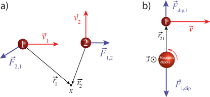
Figure 8: Two situations where action-reaction law is not obeyed in electrodynamics: a) two orthogonality moving point charges (Feynman paradox); b) interaction of a magnetic dipole with a particle of the cloud. In a), the electric forces each particle exerts on the other are nearly opposite, but particle 2 exerts a nonvanishing magnetic force $q\bm{v}_{1}\times\bm{B}_{2}$ on particle 1, whereas particle 1 does not exert any magnetic force on particle 2. In b), the force exerted by the dipole (particle 2) on the moving particle 1 is only minus half the force that the latter exerts on the former, $\bm{F}_{{\rm 1,dip}}=-2\bm{F}_{{\rm dip,1}}$.

B.1.1 Simplest example: Two moving point charges (Feynman paradox)

Consider the setup in Fig. 8a: a pair of point particles with equal charge $q$ and mass $M$, and with orthogonal velocities, one (particle 1) moving directly towards the other with $\bm{v}_{1}=v_{1}\bm{e}_{x}$, and the other moving orthogonally with $\bm{v}_{2}=v_{2}\bm{e}_{y}$. To first “post-Coulombian” Will:1993ns ; Costa:2016iwu ; Gralla:2010xg order, the electric and magnetic fields generated by a moving charge are Costa:2016iwu (cf. also Will:1993ns ; Jackson:1998nia )

$$\bm{E}_{{\rm a}}=q(1+\varphi_{{\rm a}})\frac{\bm{r}_{{\rm a}}}{r_{{\rm a}}^{3}}-\frac{1}{2}q\frac{\bm{a}_{{\rm a}}}{r_{{\rm a}}};\qquad\bm{B}_{{\rm a}}=\frac{q}{r_{{\rm a}}^{3}}\bm{v}_{{\rm a}}\times\bm{r}_{{\rm a}}$$ (114)

where $\bm{r}_{{\rm a}}\equiv\bm{x}-\bm{x}_{{\rm a}}$, $\bm{x}$ is the point of observation, $\bm{x}_{{\rm a}}$ is the instantaneous position of particle “${\rm a}$”, $\bm{a}_{{\rm a}}$ its acceleration, and

$$\varphi_{{\rm a}}\equiv\frac{v_{{\rm a}}^{2}}{2}-\frac{1}{2}(\bm{r}_{{\rm a}}\cdot\bm{a}_{{\rm a}})-\frac{3}{2}\frac{(\bm{r}_{{\rm a}}\cdot\bm{v}_{{\rm a}})^{2}}{r_{{\rm a}}^{2}}\ .$$

For a system of two bodies, to 1PC accuracy, $\bm{a}_{{\rm a}}$ in the equation above is to be taken as the Coulomb force caused by the other body, divided by the mass: $\bm{a}_{{\rm a}}=(q^{2}/M)\bm{r}_{12}/r_{12}^{3}$. The electric force exerted by particle 1 on particle 2 is then

$$\bm{F}_{{\rm EL1,2}}=q\bm{E}_{1}=q^{2}(1+\varphi_{1}-\frac{q^{2}}{2Mr_{12}})\frac{\bm{r}_{12}}{r_{12}^{3}}$$

and its reciprocal, the force $\bm{F}_{{\rm EL2,1}}=q\bm{E}_{2}$ exerted by particle 2 on particle 1, is

$$\bm{F}_{{\rm EL2,1}}=q^{2}(1+\varphi_{2}-\frac{q^{2}}{2Mr_{21}})\frac{\bm{r}_{21}}{r_{21}^{3}}=-q^{2}(1+\varphi_{2}-\frac{q^{2}}{2Mr_{12}})\frac{\bm{r}_{12}}{r_{12}^{3}}$$

where we noted that $\bm{r}_{12}\equiv\bm{r}_{1}-\bm{r}_{2}=-\bm{r}_{21}$. Thus, the electric forces are of opposite direction and of nearly equal magnitude: $\bm{F}_{{\rm EL1,2}}\approx-\bm{F}_{{\rm EL2,1}}$ (they slightly differ because $\varphi_{1}\neq\varphi_{2}$). The same however does not apply to the magnetic forces: particle 1 exerts no magnetic force on particle 2, $\bm{F}_{{\rm M1,2}}=0$, since, at the site of particle 2, $\bm{B}_{1}=q\bm{v}_{1}\times\bm{r}_{12}/r_{12}^{3}=0$, whereas particle 2 exerts a nonvanishing magnetic force on particle 1:

$$\bm{F}_{{\rm M2,1}}=q\bm{v}_{1}\times\bm{B}_{2}=-\frac{q^{2}v_{1}v_{2}}{r_{12}^{2}}\bm{e}_{y}\ .$$

Therefore

$$\bm{F}_{1,2}=\bm{F}_{{\rm EL1,2}}\neq\bm{F}_{2,1}=\bm{F}_{{\rm EL2,1}}+\bm{F}_{{\rm M2,1}}$$

showing that an action-reaction law (in a naive Newtonian sense) does not apply here. This example, sometimes called the “Feynman paradox,” is due to Feynman, see Ref. Feynman:1963uxa p. 26-5 and 27-11, and Fig. 26-6 therein. Further discussions on this problem are given in e.g Sec. 8.2.1 of Ref. GriffithsBook , and, in more detail, in Ref. PageAdams .

B.1.2 Interaction of a magnetic dipole with individual particles of the cloud

Consider a system composed of a magnetic dipole $\bm{\mu}=\mu\bm{e}_{z}$ placed at the origin (call it particle 2), and a particle of the cloud (particle 1, of charge $q$) in the equatorial plane, and at the instantaneous position depicted in Fig. 8b. The magnetic field created by the magnetic dipole is given by Eq. (21) ; the force it exerts on particle 1 is thus

$$\bm{F}_{{\rm dip,1}}=q\bm{v}\times\bm{B}_{{\rm dip}}=-q\frac{\bm{v}\times\bm{\mu}}{r_{21}^{3}}=q\frac{v\mu}{r_{21}^{3}}\bm{e}_{y}\ .$$ (115)

Let us now compute the force that particle 1 exerts on the dipole. The magnetic field created by a generically moving charge is, from Eq. (114), $\bm{B}_{{\rm charge}}=q\bm{v}\times\bm{r}/r^{3}$; the force it exerts on the dipole is $F_{{\rm charge,dip}}^{i}=B_{{\rm charge}}^{j,i}\mu_{j}\equiv\nabla^{i}(\bm{\mu}\cdot\bm{B}_{{\rm charge}})$, cf. Eqs. (4)-(5); explicitly:

$$\bm{F}_{{\rm charge,dip}}=q\frac{\bm{\mu}\times\bm{v}}{r^{3}}-3q\frac{(\bm{v}\times\bm{r})\cdot\bm{\mu}}{r^{5}}\bm{r}\ .$$ (116)

Hence, the force exerted by particle 1 on the dipole is

$$\bm{F}_{{\rm 1,dip}}=q\frac{\bm{\mu}\times\bm{v}}{r_{21}^{3}}-3q\frac{(\bm{v}\times\bm{r}_{12})\cdot\bm{\mu}}{r_{21}^{5}}\bm{r}_{12}=-\frac{2v\mu q}{r_{21}^{3}}\bm{e}_{y}\ .$$

Comparing with Eq. (115), again we see that action does not meet reaction: $\bm{F}_{{\rm 1,dip}}=-2\bm{F}_{{\rm dip,1}}$ (the sign is opposite as expected, but the magnitudes do not meet).

Let us now consider particle 3 lying at $\bm{x}_{3}=r_{3}\bm{e}_{z}$, and moving (again) with velocity $\bm{v}=v\bm{e}_{x}$. The force that the dipole exerts on it, $\bm{F}_{{\rm dip,3}}=q\bm{v}\times\bm{B}_{{\rm dip}}(x_{3})$, is, from Eq. (21),

$$\bm{F}_{{\rm dip,3}}=-q\frac{\bm{v}\times\bm{\mu}}{r_{23}^{3}}+q\frac{3(\bm{\mu}\cdot\bm{r}_{23})\bm{v}\times\bm{r}_{23}}{r_{23}^{5}}=-2\frac{v\mu q}{r_{23}^{3}}\bm{e}_{y}\ .$$

Its reciprocal (the force that particle 3 exerts on the dipole) is, from Eq. (116),

$$\bm{F}_{{\rm 3,dip}}=q\frac{\bm{\mu}\times\bm{v}}{r_{23}^{3}}-3q\frac{(\bm{v}\times\bm{r}_{32})\cdot\bm{\mu}}{r_{23}^{5}}\bm{r}_{32}=\frac{v\mu q}{r_{23}^{3}}\bm{e}_{y}$$

since the second term of the second expression vanishes. Thus, again, action does not meet reaction, only now it is the magnitude of the force on the particle that is twice that on the dipole: $\bm{F}_{{\rm dip,3}}=-2\bm{F}_{{\rm 3,dip}}$.

B.1.3 A magnetic dipole and an infinite straight wire

Consider again a magnetic dipole $\bm{\mu}=\mu\bm{e}_{z}$ placed at the origin, and an infinitely long wire placed along the straightline (parallel to the $x$ axis) defined by $y=y_{0}$, $z=0$, with a current $\bm{I}=\Sigma\bm{j}$ flowing through it in the positive $x$ direction, $\bm{j}=j\bm{e}_{x}$. $\Sigma$ is the cross sectional area of the wire. The force exerted by the magnetic dipole (placed at the origin, and with $\bm{\mu}=\mu\bm{e}_{z}$) on the wire is, from Eq. (21),

$$\bm{F}_{{\rm dip,wire}}=\int_{{\rm wire}}\bm{j}\times\bm{B}_{{\rm dip}}=-\int_{{\rm wire}}\frac{\bm{j}\times\bm{\mu}}{r^{3}}=\frac{2\mu I}{y_{0}^{2}}\bm{e}_{y}.$$

Let us now compute its reciprocal, i.e. the force that the wire exerts on the dipole. The magnetic field generated by the wire is well known to be (e.g. Sec. 5.3 of GriffithsBook , or Eqs. (14.22)-(14.24) of Feynman:1963uxa )

$$\bm{B}_{{\rm wire}}=\frac{2I}{(z^{2}+y^{\prime 2})}\left[y^{\prime}\bm{e}_{z}-z\bm{e}_{y}\right]$$

where $y^{\prime}=y-y_{0}$. Thus $B_{{\rm wire}}^{i,j}$ has the only nonvanishing components $B_{{\rm wire}}^{z,y}=B_{{\rm wire}}^{y,z}=2I(z^{2}-y^{\prime 2})(z^{2}+y^{\prime 2})^{-2}$. Therefore, the force exerted on the dipole, $\bm{F}_{{\rm wire,dip}}=B_{{\rm wire}}^{j,i}\mu_{j}\bm{e}_{i}\equiv\nabla(\bm{\mu}\cdot\bm{B}_{{\rm wire}})$, is

$$\bm{F}_{{\rm wire,dip}}=-\frac{2\mu I}{y_{0}^{2}}\bm{e}_{y}=-\bm{F}_{{\rm dip,wire}}\ .$$

So, in this case, the action-reaction law is obeyed, just like for the current slabs in Sec. II.1. This is the expected result because one is dealing here with magnetostatics, where there cannot be an exchange between mechanical and field momentum, for the latter is constant and equal to zero (the Poynting vector is zero, since the electric field is zero).

B.2 Gravitomagnetism

Analogous examples to the ones above can be given in gravity — two point masses momentarily in orthogonal motion, the interaction of the spinning body with individual particles of the cloud (Sec. III.2.2), and with the entire cloud — with entirely analogous conclusions. (As for the infinite wire of Sec. B.1.3, it cannot be mirrored here since the metric of an infinitely long cylindrical mass is not asymptotically flat). Below we discuss in detail the especially important second example.

B.2.1 Interaction of a spinning body with individual particles of the cloud

Consider a system composed of a spinning body momentarily at rest (body 2, of mass $M_{2}$, and angular momentum $\bm{S}$), and a point mass (body 1, of mass $M_{1}$) moving with velocity $\bm{v}_{1}=\bm{v}$, as illustrated in Fig. 9.

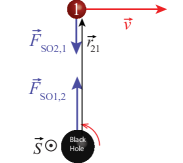
Figure 9: A situation where the action reaction law is not obeyed in PN gravity (analogue of Fig. 8b): the spin-orbit force $\bm{F}_{{\rm SO}2,1}$ exerted by the spinning body (e.g. a BH) on a moving particle is not the same as the spin-orbit force $\bm{F}_{{\rm SO}1,2}$ that the latter exerts on the former: $\bm{F}_{{\rm SO}1,2}=-3\bm{F}_{{\rm SO}2,1}/2$.

To 1.5PN order, the coordinate acceleration of a (spinning or nonspinning) body in a gravitational field is generically given by Eqs. (44), (40), (46). The coordinate acceleration of the spinning body (body 2), due to the gravitational field generated by the moving point mass 1, is then (since $\bm{v}_{2}=0$)

$$\frac{d^{2}\bm{x}_{2}}{dt^{2}}=(1-2U_{1})\bm{G}_{1}+\frac{1}{M_{2}}\bm{F}$$ (117)

where $U_{1}=M_{1}/r_{1}$ is the Newtonian potential of body 1 and $\bm{F}$ is the spin-curvature force on body 2. The latter amounts to the whole spin-orbit force that acts on body 2, so we may write $\bm{F}=\bm{F}_{{\rm SO}1,2}$. From Eq. (40),

$$F_{{\rm SO}1,2}^{j}=F^{j}=\frac{1}{2}H_{1}^{i,j}S_{i}-(\bm{S}\times\dot{\bm{G}}_{1})^{j}\ .$$ (118)

Here $\bm{H}_{1}$ is the gravitomagnetic field generated by the translational motion of body 1; it is given by $\bm{H}_{1}=\nabla\times\bm{\mathcal{A}_{1}}$, with $\bm{\mathcal{A}_{1}}=-4M_{1}\bm{v}/r_{1}$ (cf. e.g. Costa:2016iwu ; Kaplan:2009 ), or, explicitly

$$\bm{H}_{1}=-4\frac{M_{1}}{r_{1}^{3}}\bm{v}\times\bm{r}_{1}$$ (119)

The gravitoelectric field $\bm{G}_{1}$, to the accuracy at hand, is to be taken, in this expression, as the leading term $\bm{G}_{1}\simeq-M\bm{r}_{1}/r_{1}^{3}$. In order to compute $\dot{\bm{G}}_{1}$, one notes that $\dot{\bm{r}}_{1}=-\bm{v}$, and that $\dot{r}_{1}=-\bm{r}_{1}\cdot\bm{v}/r_{1}$. One gets

$$\bm{F}_{{\rm SO}1,2}=$$

$$\frac{3M_{1}}{r_{12}^{3}}\left[\bm{v}\times\bm{S}+\frac{2\bm{r}_{12}[(\bm{v}\times\bm{r}_{12})\cdot\bm{S}]}{r_{12}^{2}}+\frac{(\bm{v}\cdot\bm{r}_{12})\bm{S}\times\bm{r}_{12}}{r_{12}^{2}}\right].$$ (120)

Notice that this amounts to the whole spin-orbit force that acts on body 2: $\bm{F}_{{\rm SO}1,2}=\bm{F}$.

The coordinate acceleration of body 1 (the point mass) is, from Eqs. (44)-(46),

$$\frac{d^{2}\bm{x}_{1}}{dt^{2}}=(1+v^{2}-2U_{2})\bm{G}_{2}-4(\bm{G}_{2}\cdot\bm{v})\bm{v}+\bm{v}\times\bm{H}_{2}$$ (121)

where $U_{2}=M_{2}/r_{2}$ is the Newtonian potential of the spinning body ($\bm{F}=0$ in this case, since body 1’s spin is zero). The gravitomagnetic field $\bm{H}_{2}$ generated by the spinning body 2 is given by Eq. (55) (replacing therein $\bm{r}\rightarrow\bm{r}_{2}$); therefore the gravitomagnetic “force” $M_{1}\bm{v}\times\bm{H}_{2}$ it exerts on body 1, which amounts to the whole spin-orbit force $\bm{F}_{{\rm SO}2,1}$ acting on body 1, is given by

$$\bm{v}\times\bm{H}_{2}=\frac{1}{r_{12}^{3}}\left[2\bm{v}\times\bm{S}-\frac{6}{r_{12}^{2}}(\bm{r}_{21}\cdot\bm{S})\bm{v}\times\bm{r}_{21}\right]=\frac{\bm{F}_{{\rm SO}2,1}}{M_{1}}\ .$$ (122)

Using the vector identity (5.2a) of Faye:2006gx , we can re-write this result as

$$\bm{F}_{{\rm SO}2,1}=$$

$$-\frac{3M_{1}}{r_{12}^{3}}\left[\frac{4}{3}\bm{v}\times\bm{S}+\frac{2\bm{r}_{12}[(\bm{v}\times\bm{r}_{12})\cdot\bm{S}]}{r_{12}^{2}}+\frac{2(\bm{v}\cdot\bm{r}_{12})\bm{S}\times\bm{r}_{12}}{r_{12}^{2}}\right],$$ (123)

cf. Eq. (5.3a) of Faye:2006gx . Comparing with (120), we see that the spin-orbit interactions do not obey an action-reaction law: $\bm{F}_{{\rm SO}1,2}\neq-\bm{F}_{{\rm SO}2,1}$. In other words, the spin-curvature force (120) exerted by body 1 on body 2, is different from the gravitomagnetic “force” (122) exerted by body 2 on body 1. Notice that $\bm{F}_{{\rm SO}1,2}$ is the analogue of the electromagnetic force $\bm{F}_{1,{\rm dip}}$ of Sec. B.1.2, and $\bm{F}_{{\rm SO}2,1}$ the analogue of $\bm{F}_{{\rm dip,1}}$. Therefore, the overall coordinate accelerations of the two bodies do not likewise obey an action-reaction law:

$$M_{2}\frac{d^{2}\bm{x}_{2}}{dt^{2}}\neq M_{1}\frac{d^{2}\bm{x}_{1}}{dt^{2}}\ .$$

In fact, comparing (117) to (121), we see that actually all the PN terms (not only the spin-orbit ones) differ; only the Newtonian parts of $M_{1}\bm{G}_{2}$ and $M_{2}\bm{G}_{1}$ match up to sign.

For the setup in Fig. 9, where particle 1 lies in the equatorial plane at the instantaneous position $\bm{x}_{1}=r_{1}\bm{e}_{z}$, and has velocity $\bm{v}_{1}=\bm{v}=v\bm{e}_{x}$, we have

$$\bm{F}_{{\rm SO}1,2}=\frac{3M_{1}}{r_{12}^{3}}\left[\bm{v}\times\bm{S}+\frac{2\bm{r}_{12}[(\bm{v}\times\bm{r}_{12})\cdot\bm{S}]}{r_{12}^{2}}\right]=\frac{3M_{1}Sv}{r_{12}^{3}}\bm{e}_{y}$$ (124)

and

$$\bm{F}_{{\rm SO}2,1}=M_{1}\bm{v}\times\bm{H}_{2}=\frac{2}{r_{12}^{3}}M_{1}\bm{v}\times\bm{S}=-\frac{2M_{1}Sv}{r_{12}^{3}}\bm{e}_{y}\ .$$ (125)

Therefore, $\bm{F}_{{\rm SO}1,2}=-3\bm{F}_{{\rm SO}2,1}/2$.

Let us now consider particle 3 lying at $\bm{x}_{3}=r_{3}\bm{e}_{z}$ (i.e., on top of the spinning body, above the equatorial plane), and, again, with velocity $\bm{v}_{3}=\bm{v}=v\bm{e}_{x}$, see Fig. 1b. The spin-orbit force that it exerts on the spinning body, $\bm{F}_{{\rm SO}3,2}=\bm{F}$, is obtained from Eq. (120), replacing therein $\bm{r}_{12}\rightarrow\bm{r}_{32}$, with $\bm{r}_{32}\equiv\bm{r}_{3}-\bm{r}_{2}$,

$$\bm{F}_{{\rm SO}3,2}=\frac{3M_{3}}{r_{32}^{3}}\left[\bm{v}\times\bm{S}+\frac{2\bm{r}_{32}[(\bm{v}\times\bm{r}_{32})\cdot\bm{S}]}{r_{32}^{2}}\right]=-\frac{3M_{3}Sv}{r_{23}^{3}}\bm{e}_{y}\ ,$$ (126)

where we noted that $(\bm{v}\times\bm{r}_{32})\cdot\bm{S}=0$. The spin-orbit force exerted by the spinning body on particle 3, $\bm{F}_{{\rm SO}2,3}=M_{3}\bm{v}\times\bm{H}_{{\rm 2}}$, is

$$\bm{F}_{{\rm SO}2,3}=\frac{2M_{3}}{r_{23}^{3}}\left[\bm{v}\times\bm{S}-\frac{3}{r_{23}^{2}}(\bm{r}_{23}\cdot\bm{S})\bm{v}\times\bm{r}_{23}\right]=\frac{4M_{3}Sv}{r_{23}^{3}}\bm{e}_{y}.$$ (127)

Thus, again, action does not equal minus reaction: $\bm{F}_{{\rm SO}2,3}=-4\bm{F}_{{\rm SO}3,2}/3$.

Analogously to the electromagnetic case, this mismatch between action and reaction does not mean a violation of any conservation principle; it can be cast as an interchange between mechanical momentum of the bodies and field momentum (in the sense of the Landau-Lifshitz pseudotensor, see Kaplan:2009 ). It is the same principle that is behind the famous bobbings in binary systems Keppel:2009tc , where the center of mass of the whole binary bobs up and down.

The examples above illustrate an important aspect depicted in Fig. 1b: cloud particles in the equatorial plane deflect in the negative $y$ direction (i.e., to the left in Fig. 1b), cf. Eq. (125), and push the spinning body to the right, as Eq. (124) shows; however, cloud particles in regions outside the equatorial plane do the opposite: they deflect to the right [cf. Eq. (127)], and push the spinning body to the left, with a force whose magnitude is twice that of the force exerted by the particles at the equatorial plane, as shown by Eq. (126). It is the effect of the latter that eventually prevails in the cloud slab (orthogonal to $y$) of Fig. 3, where the net force on the cloud points in the positive $y$ direction (and the force on the spinning body points in the negative $y$ direction), whereas in the special case of a slab orthogonal to $z$ (i.e., to the body’s spin axis) the two effects exactly cancel out.

The above explains also why in the earlier work Okawa:2014sxa the authors were misled into concluding that the force on the spinning body was opposite to the Magnus effect (“anti-Magnus”, upwards in Fig. 3): the argument therein is based on the asymmetric accretion that occurs in a spinning BH, i.e., the absorption cross section being larger for counterrotating particles than for corotating ones. This is a gravitomagnetic phenomenon, due to the fact that the gravitomagnetic force $\bm{F}_{{\rm GM}}=M\bm{v}\times\bm{H}$ is attractive for counterrotating particles, and repulsive in the corotating case. That can easily be seen considering again particles with velocity $\bm{v}=v\bm{e}_{x}$, as in Fig. 1b; from Eq. (55), it follows that the radial component of the gravitomagnetic force is $\bm{F}_{{\rm GM}}\cdot\bm{r}/r=-2MvSy/r^{4}$ (attractive for positive $y$, repulsive for negative $y$). However, it is crucial here to distinguish between the radial component of $\bm{F}_{{\rm GM}}$ (which determines its attractive/repulsive nature), from the force itself, and the overall deflection it causes. If one looks only at the equatorial plane, the reasoning in Okawa:2014sxa is qualitatively correct, since, as depicted in Fig. 1b, particles in the equatorial plane suffer a deflection opposite to that corresponding to a Magnus effect. That however overlooks the key fact that, as exemplified by the particles along the axis in Fig. 1b, there are regions outside the equatorial plane where particles are deflected in the opposite direction, i.e., in the direction expected from a Magnus effect.

References

- (1) S. I. Rubinow and J. B. Keller, “The transverse force on a spinning sphere moving in a viscous fluid,” Journal of Fluid Mechanics 11 no. 3, (1961) 447.
- (2) Y. Tsuji, Y. Morikawa, and O. Mizuno, “Experimental measurement of the Magnus force on a rotating sphere at low Reynolds numbers,” J. Fluids Eng. 107 (1985) 484.
- (3) R. G. Watts and R. Ferrer, “The lateral force on a spinning sphere: Aerodynamics of a curveball,” American Journal of Physics 55 no. 1, (1987) 40.
- (4) B. Munson, D. Young, and T. Okiishi, Fundamentals of fluid mechanics. Wiley & Sons, 1998.
- (5) I. Ciufolini and J. A. Wheeler, Gravitation and Inertia. Princeton Series in Physics, Princeton, NJ, 1995.
- (6) J. A. Font, J. M. Ibanez, and P. Papadopoulos, “Nonaxisymmetric relativistic Bondi-Hoyle accretion onto a Kerr black hole,” Mon. Not. Roy. Astron. Soc. 305 (1999) 920, arXiv:astro-ph/9810344 [astro-ph].
- (7) H. Okawa and V. Cardoso, “Black holes and fundamental fields: Hair, kicks, and a gravitational Magnus effect,” Phys. Rev. D90 no. 10, (2014) 104040, arXiv:1405.4861 [gr-qc].
- (8) B. Cashen, A. Aker, and M. Kesden, “Gravitomagnetic dynamical friction,” Phys. Rev. D95 no. 6, (2017) 064014, arXiv:1610.01590 [gr-qc].
- (9) M. Mathisson, “Neue mechanik materieller systemes,” Acta Phys. Polon. 6 (1937) 163.
- (10) A. Papapetrou, “Spinning test particles in general relativity. 1.,” Proc. Roy. Soc. Lond. A209 (1951) 248–258.
- (11) W. G. Dixon, “A covariant multipole formalism for extended test bodies in general relativity,” Il Nuovo Cimento 34 (1964) 317.
- (12) W. G. Dixon, “Dynamics of extended bodies in general relativity. I. Momentum and angular momentum,” Proc. Roy. Soc. Lond. A314 (1970) 499–527.
- (13) S. E. Gralla, A. I. Harte, and R. M. Wald, “Bobbing and Kicks in Electromagnetism and Gravity,” Phys. Rev. D81 (2010) 104012, arXiv:1004.0679 [gr-qc].
- (14) W. Tulczyjew, “Motion of multipole particles in general relativity theory,” Acta Phys. Polon. 18 (1959) 393.
- (15) L. F. O. Costa, J. Natário, and M. Zilhão, “Spacetime dynamics of spinning particles: Exact electromagnetic analogies,” Phys. Rev. D93 no. 10, (2016) 104006, arXiv:1207.0470 [gr-qc].
- (16) L. Filipe Costa and C. A. R. Herdeiro, “Gravitoelectromagnetic analogy based on tidal tensors,” Phys. Rev. D78 (2008) 024021.
- (17) L. F. O. Costa, L. Wylleman, and J. Natário, “Gravitomagnetism and the significance of the curvature scalar invariants,” arXiv:1603.03143 [gr-qc].
- (18) D. J. Griffiths, Introduction to electrodynamics. Pearson Benjamim Cummings, San Francisco, 2008.
- (19) J. D. Jackson, Classical Electrodynamics. Wiley, 1998.
- (20) {https://en.wikipedia.org/wiki/Fubini_theorem}.
- (21) P. Walker, Examples and Theorems in Analysis. Springer-Verlag, London, 2004.
- (22) L. F. O. Costa and J. Natário, “Center of mass, spin supplementary conditions, and the momentum of spinning particles,” in Equations of Motion in Relativistic Gravity, D. Puetzfeld, C. Lämmerzahl, and B. Schutz, eds., pp. 215–258. Springer, Cham, 2015 [Fund. Theor. Phys. 179, 215]. arXiv:1410.6443.
- (23) F. A. E. Pirani, “On the physical significance of the Riemann tensor,” Acta Phys. Polon. 15 (1956) 389–405. [Gen. Relativ. Gravit. 41,1215 (2009)].
- (24) N. Dadhich, “Electromagnetic duality in general relativity,” Gen. Rel. Grav. 32 (2000) 1009–1023, arXiv:gr-qc/9909067 [gr-qc].
- (25) G. F. R. Ellis, R. Maartens, and M. A. H. MacCallum, Relativistic Cosmology. Cambridge University Press, Cambridge, UK, 2012.
- (26) R. Maartens and B. A. Bassett, “Gravito-electromagnetism,” Classical and Quantum Gravity 15 no. 3, (1998) 705.
- (27) T. Damour, M. Soffel, and C.-m. Xu, “General relativistic celestial mechanics. 1. Method and definition of reference systems,” Phys. Rev. D43 (1991) 3272–3307.
- (28) E. Poisson and C. M. Will, Gravity: Newtonian, Post-Newtonian, Relativistic. Cambridge University Press, Cambridge, UK, 2014.
- (29) C. W. Misner, K. S. Thorne, and J. A. Wheeler, Gravitation. W. H. Freeman, San Francisco, 1973.
- (30) C. M. Will, Theory and experiment in gravitational physics. Cambridge University Press, Cambridge, UK, 1993.
- (31) J. D. Kaplan, D. A. Nichols, and K. S. Thorne, “Post-Newtonian approximation in Maxwell-like form,” Phys. Rev. D80 (2009) 124014, arXiv:0808.2510 [gr-qc].
- (32) D. Bini, P. Carini, R. T. Jantzen, and D. Wilkins, “Thomas precession in post-Newtonian gravitoelectromagnetism,” Phys. Rev. D 49 (1994) 2820–2827.
- (33) L. F. O. Costa, G. Lukes-Gerakopoulos, and O. Semerák, “Spinning particles in general relativity: Momentum-velocity relation for the Mathisson-Pirani spin condition,” Phys. Rev. D97 (2018) 084023, arXiv:1712.07281 [gr-qc].
- (34) R. M. Wald, “Gravitational spin interaction,” Phys. Rev. D6 (1972) 406–413.
- (35) L. F. Costa and J. Natário, “The Coriolis field,” Am. J. Phys. 84 (2016) 388, arXiv:1511.02458.
- (36) P. Vickers, “Was Newtonian cosmology really inconsistent?,” Studies in History and Philosophy of Science Part B: Studies in History and Philosophy of Modern Physics 40 (2009) 197 – 208.
- (37) W. H. McCrea, “On the significance of Newtonian cosmology,” Astronom. Journal 60 (1955) 271.
- (38) C. O’Raifeartaigh, M. O’Keeffe, W. Nahm, and S. Mitton, “Einstein’s 1917 static model of the universe: a centennial review,” European Physical Journal H 42 (2017) 431–474, arXiv:1701.07261.
- (39) H. Lorentz, A. Einstein, H. Minkowski, and H. Weyl, The priciple Relativity: A Collection of Original Memoirs on the Special and General Theory of Relativity. Dover Publications, Inc, New York, 1952.
- (40) A. Einstein, Relativity: The special and the general theory, R.W. Lawson(trans.). Methuen, London, 1954.
- (41) J. Binney and S. Tremaine, Galactic Dynamics: Second Edition. Princeton University Press, 2008.
- (42) G. Bertone and D. Merritt, “Time-dependent models for dark matter at the Galactic Center,” Phys. Rev. D72 (2005) 103502, arXiv:astro-ph/0501555 [astro-ph].
- (43) A. Burkert, “The Structure of dark matter halos in dwarf galaxies,” Astrophys. J. 447 (1995) L25, arXiv:astro-ph/9504041 [astro-ph].
- (44) O. B. Karpov, “Gyroscope deviation from geodesic motion: Quasiresonant oscillations on a circular orbit,” J. Exp. Theor. Phys. 96 (2003) 581–586, arXiv:gr-qc/0301056 [gr-qc]. [Zh. Eksp. Teor. Fiz. 123, 659 (2003)].
- (45) E. Barausse, V. Cardoso, and P. Pani, “Can environmental effects spoil precision gravitational-wave astrophysics?,” Phys. Rev. D89 no. 10, (2014) 104059, arXiv:1404.7149.
- (46) C. Møller, “Sur la dynamique des systèmes ayant un moment angulaire interne,” Annales de l’institut Henri Poincaré 11 no. 5, (1949) 251–278.
- (47) P. Pani, “Binary pulsars as dark-matter probes,” Phys. Rev. D92 no. 12, (2015) 123530, arXiv:1512.01236.
- (48) J. I. Read, “The Local Dark Matter Density,” J. Phys. G41 (2014) 063101, arXiv:1404.1938 [astro-ph.GA].
- (49) G. Gilmore, “The distribution of dark matter in the Milky Way galaxy,” in Proceedings, 1st International Workshop on The identification of dark matter (IDM 1996): Sheffield, UK, September 8-12, 1996, pp. 73–82. World Scientific, Singapore, 1997. arXiv:astro-ph/9702081 [astro-ph].
- (50) R. Komm, R. Howe, B. R. Durney, and F. Hill, “Temporal Variation of Angular Momentum in the Solar Convection Zone,” ApJ 586 (2003) 650–662.
- (51) R. P. van der Marel and N. Kallivayalil, “Third-Epoch Magellanic Cloud Proper Motions II: The Large Magellanic Cloud Rotation Field in Three Dimensions,” Astrophys. J. 781 no. 2, (2014) 121, arXiv:1305.4641 [astro-ph.CO].
- (52) http://sci.esa.int/gaia/.
- (53) R. Genzel et al., “The stellar cusp around the supermassive black hole in the galactic center,” Astrophys. J. 594 no. 2, (2003) 812, arXiv:astro-ph/0305423.
- (54) I. D. Novikov and K. S. Thorne, “Astrophysics of black holes.,” in Black Holes (Les Astres Occlus), C. Dewitt and B. S. Dewitt, eds., pp. 343–450. Gordon and Breach, New York, 1973.
- (55) N. I. Shakura and R. A. Sunyaev, “Black holes in binary systems. Observational appearance,” Astron. Astrophys. 24 (1973) 337–355.
- (56) K. Nordtvedt, “Existence of the Gravitomagnetic Interaction,” Int. J. Theor. Phys. 27 (1988) 1395–1404.
- (57) M. Hannam, “Modelling gravitational waves from precessing black-hole binaries: Progress, challenges and prospects,” Gen. Rel. Grav. 46 (2014) 1767, arXiv:1312.3641 [gr-qc].
- (58) R. N. Lang and S. A. Hughes, “Measuring coalescing massive binary black holes with gravitational waves: The impact of spin-induced precession,” Phys. Rev. D74 (2006) 122001, arXiv:gr-qc/0608062. [Erratum: Phys. Rev. D77,109901 (2008)].
- (59) A. Vecchio, “LISA observations of rapidly spinning massive black hole binary systems,” Phys. Rev. D70 (2004) 042001, arXiv:astro-ph/0304051.
- (60) R. N. Lang and S. A. Hughes, “Localizing coalescing massive black hole binaries with gravitational waves,” Astrophys. J. 677 (2008) 1184, arXiv:0710.3795 [astro-ph].
- (61) A. Stavridis, K. G. Arun, and C. M. Will, “Precessing supermassive black hole binaries and dark energy measurements with LISA,” Phys. Rev. D80 (2009) 067501, arXiv:0907.4686 [gr-qc].
- (62) P. Schmidt, F. Ohme, and M. Hannam, “Towards models of gravitational waveforms from generic binaries II: Modelling precession effects with a single effective precession parameter,” Phys. Rev. D91 no. 2, (2015) 024043, arXiv:1408.1810 [gr-qc].
- (63) E. Berti, A. Buonanno, and C. M. Will, “Estimating spinning binary parameters and testing alternative theories of gravity with LISA,” Phys. Rev. D71 (2005) 084025, arXiv:gr-qc/0411129 [gr-qc].
- (64) C. J. Moore, R. H. Cole, and C. P. L. Berry, “Gravitational-wave sensitivity curves,” Class. Quant. Grav. 32 no. 1, (2015) 015014, arXiv:1408.0740.
- (65) H. Audley et al., “Laser Interferometer Space Antenna,” arXiv:1702.00786 [astro-ph.IM].
- (66) G. Hobbs et al., “The international pulsar timing array project: using pulsars as a gravitational wave detector,” Classical and Quantum Gravity 27 no. 8, (2010) 084013.
- (67) S. Detweiler, “Pulsar timing measurements and the search for gravitational waves,” Astrophys. J. 234 (1979) 1100.
- (68) M. V. Sazhin, “Opportunities for detecting ultralong gravitational waves,” Soviet Astronomy 22 (1978) 36.
- (69) C. J. Moore, S. R. Taylor, and J. R. Gair, “Estimating the sensitivity of pulsar timing arrays,” Class. Quant. Grav. 32 no. 5, (2015) 055004, arXiv:1406.5199.
- (70) Z. Arzoumanian et al., “The nanograv nine-year data set: Limits on the isotropic stochastic gravitational wave background,” Astrophys. J. 821 no. 1, (2016) 13, arXiv:1508.03024.
- (71) O. Semerák and P. Suková, “Free motion around black holes with discs or rings: between integrability and chaos - I,” Mon. Not. Roy. Astron. Soc. 404 (2010) 545–574, arXiv:1211.4106 [gr-qc].
- (72) T. Morgan and L. Morgan, “The Gravitational Field of a Disk,” Phys. Rev. 183 (1969) 1097–1101. [Erratum: Phys. Rev. D 1, 3522 (1970)].
- (73) J. P. S. Lemos, “Self-similar relativistic discs with pressure,” Class. Quant. Grav. 6 (1989) 1219–1320.
- (74) J. P. S. Lemos and P. S. Letelier, “Superposition of Morgan and Morgan discs with a Schwarzschild black hole,” Class. Quant. Grav. 10 (1993) L75–L78.
- (75) J. Bicak, D. Lynden-Bell, and J. Katz, “Relativistic disks as sources of static vacuum spacetimes,” Phys. Rev. D47 no. 10, (1993) 4334.
- (76) O. A. Espitia and G. A. Gonzalez, “Relativistic static thin disks: The counterrotating model,” Phys. Rev. D68 (2003) 104028, arXiv:gr-qc/0107044 [gr-qc].
- (77) J. Bicak and T. Ledvinka, “Relativistic disks as sources of the Kerr metric,” Phys. Rev. Lett. 71 (1993) 1669–1672.
- (78) S. Nishida, Y. Eriguchi, and A. Lanza, “General Relativistic Structure of Star-Toroid Systems,” ApJ 401 (1992) 618.
- (79) P. Čížek and O. Semerák, “Perturbation of a Schwarzschild Black Hole Due to a Rotating Thin Disk,” Astrophys. J. Suppl. Ser. 232 (2017) 14, arXiv:1710.07109 [gr-qc].
- (80) P. Kotlařík, O. Semerák, and P. Čížek, “Schwarzschild black hole encircled by a rotating thin disc: Properties of perturbative solution,” Phys. Rev. D97 (2018) 084006, arXiv:1804.02010 [gr-qc].
- (81) P. Jaranowski, P. Mach, E. Malec, and M. Pirog, “General-relativistic versus Newtonian: Geometric dragging and dynamic antidragging in stationary self-gravitating disks in the first post-Newtonian approximation,” Phys. Rev. D91 no. 2, (2015) 024039, arXiv:1410.8527 [gr-qc].
- (82) M. Miyamoto and R. Nagai, “Three-dimensional models for the distribution of mass in galaxies,” Publ. Astron. Soc. Jap. 27 (1975) 533–543.
- (83) M. Baes, “Exact potential-density pairs for flattened dark haloes,” Mon. Not. Roy. Astron. Soc. 392 (2009) 1503, arXiv:0810.5483 [astro-ph].
- (84) D. Vogt and P. S. Letelier, “Analytical Potential-Density Pairs for Flat Rings and Toroidal Structures,” Mon. Not. Roy. Astron. Soc. 396 (2009) 1487, arXiv:0906.0919.
- (85) V. Witzany, O. Semerák, and P. Suková, “Free motion around black holes with discs or rings: between integrability and chaos – IV,” Mon. Not. Roy. Astron. Soc. 451 (2015) 1770, arXiv:1503.09077 [astro-ph.HE].
- (86) T. A. Apostolatos, C. Cutler, G. J. Sussman, and K. S. Thorne, “Spin induced orbital precession and its modulation of the gravitational wave forms from merging binaries,” Phys. Rev. D49 (1994) 6274–6297.
- (87) S. Babak, A. Taracchini, and A. Buonanno, “Validating the effective-one-body model of spinning, precessing binary black holes against numerical relativity,” Phys. Rev. D95 no. 2, (2017) 024010, arXiv:1607.05661 [gr-qc].
- (88) S. W. Hawking and G. F. R. Ellis, The Large Scale Structure of Space-Time. Cambridge Monographs on Mathematical Physics. Cambridge University Press, 1973.
- (89) R. M. Wald, General Relativity. The University of Chicago Press, Chicago, 1984.
- (90) P.-H. Chavanis, “Models of universe with a polytropic equation of state: II. The late universe,” EPJ Plus 129 no. 10, (2014) 222, arXiv:1208.0801.
- (91) I. Zlatev, L. Wang, and P. J. Steinhardt, “Quintessence, Cosmic Coincidence, and the Cosmological Constant,” Phys. Rev. Lett. 82 (1999) 896–899.
- (92) V. Gorini, A. Kamenshchik, U. Moschella, and V. Pasquier, “The Chaplygin gas as a model for dark energy,” in On recent developments in theoretical and experimental general relativity, gravitation, and relativistic field theories. Proceedings, 10th Marcel Grossmann Meeting, MG10, Rio de Janeiro, Brazil, July 20-26, 2003. Pt. A-C, pp. 840–859. World Scientific, Singapore, 2006. arXiv:gr-qc/0403062.
- (93) A. Vikman, “Can dark energy evolve to the phantom?,” Phys. Rev. D71 (2005) 023515, arXiv:astro-ph/0407107.
- (94) C. L. Bennett et al., “Nine-year Wilkinson Microwave Anisotropy Probe (WMAP) Observations: Final Maps and Results,” Astrophys. J. Suppl. Ser. 208 no. 2, (2013) 20.
- (95) C. M. Springob et al., “SFI++ II: A New I-band Tully-Fisher Catalog, Derivation of Peculiar Velocities and Dataset Properties,” Astrophys. J. Suppl. Ser. 172 (2007) 599–614, arXiv:0705.0647 [astro-ph]. [Erratum: Astrophys. J. Suppl. Ser. 182, 474 (2009)].
- (96) R. P. Feynman, R. B. Leighton, and M. Sands, The Feynman Lectures on Physics, Vol. II. Addison Wesley, 1964. http://www.feynmanlectures.info/.
- (97) L. Page and N. I. Adams, “Action and Reaction Between Moving Charges,” Am. J. Phys. 13 (1945) 141–147.
- (98) G. Faye, L. Blanchet, and A. Buonanno, “Higher-order spin effects in the dynamics of compact binaries. I. Equations of motion,” Phys. Rev. D74 (2006) 104033, arXiv:gr-qc/0605139 [gr-qc].
- (99) D. Keppel, D. A. Nichols, Y. Chen, and K. S. Thorne, “Momentum Flow in Black Hole Binaries. I. Post-Newtonian Analysis of the Inspiral and Spin-Induced Bobbing,” Phys. Rev. D80 (2009) 124015, arXiv:0902.4077 [gr-qc].