Detection of Unknown Anomalies in Streaming Videos with Generative Energy-based Boltzmann Models

Abstract

Abnormal event detection is one of the important objectives in research and practical applications of video surveillance. However, there are still three challenging problems for most anomaly detection systems in practical setting: limited labeled data, ambiguous definition of “abnormal” and expensive feature engineering steps. This paper introduces a unified detection framework to handle these challenges using energy-based models, which are powerful tools for unsupervised representation learning. Our proposed models are firstly trained on unlabeled raw pixels of image frames from an input video rather than hand-crafted visual features; and then identify the locations of abnormal objects based on the errors between the input video and its reconstruction produced by the models. To handle video stream, we develop an online version of our framework, wherein the model parameters are updated incrementally with the image frames arriving on the fly. Our experiments show that our detectors, using Restricted Boltzmann Machines (RBMs) and Deep Boltzmann Machines (DBMs) as core modules, achieve superior anomaly detection performance to unsupervised baselines and obtain accuracy comparable with the state-of-the-art approaches when evaluating at the pixel-level. More importantly, we discover that our system trained with DBMs is able to simultaneously perform scene clustering and scene reconstruction. This capacity not only distinguishes our method from other existing detectors but also offers a unique tool to investigate and understand how the model works.

Georgia Institute of Technology, Atlanta, GA, 30332 USA e-mail: (see http://www.michaelshell.org/contact.html).

I Introduction

In the last few years, the security and safety concerns in public places and restricted areas have increased the need for visual surveillance. Large distributed networks of many high quality cameras have been deployed and producing an enormous amount of data every second. Monitoring and processing such huge information manually are infeasible in practical applications. As a result, it is imperative to develop autonomous systems that can identify, highlight, predict anomalous objects or events, and then help to make early interventions to prevent hazardous actions (e.g., fighting or a stranger dropping a suspicious case) or unexpected accidents (e.g., falling or a wrong movement on one-way streets). Video anomaly detection can also be widely-used in variety of applications such as restricted-area surveillance, traffic analysis, group activity detection, home security to name a few. The recent studies [1] show that video anomaly detection has received considerable attention in the research community and become one of the essential problems in computer vision. However, deploying surveillance systems in real-world applications poses three main challenges: a) the easy availability of unlabeled data but lack of labeled training data; b) no explicit definition of anomaly in real-life video surveillance and c) expensive hand-crafted feature extraction exacerbated by the increasing complexity in videos.

The first challenge comes from the fast growing availability of low-cost surveillance cameras nowadays. A typical RGB camera with the resolution of $340\times 640$ pixels can add more than one terabyte video data every day. To label this data, an annotation process is required to produce a ground-truth mask for every video frame. In particular, a person views the video, stops at a frame and then assigns pixel regions as anomalous objects or behaviors wherever applicable. This person has to be well-trained and carefully look at every single detail all the time, otherwise he might miss some unusual events that suddenly appear. This process is extremely labor-intensive, rendering it impossible to obtain large amount of labeled data; and hence upraising the demand for a method that can exploit the overabundant unlabeled videos rather than relying on the annotated one.

The second challenge of no explicit definition is due to the diversity of abnormal events in reality. In some constrained environments, abnormalities are well-defined, for example, putting goods into pocket in the supermarket [2]; hence we can view the problem as activity recognition and apply a machine learning classifier to detect suspicious behaviors. However, anomaly objects in most scenarios are undefined, e.g., any objects except for cars on free-way can be treated as anomaly. Therefore, an anomaly detection algorithm faces the fact that it has scarce information about what it needs to predict until they actually appear. As a result, developing a good anomaly detector to detect unknown anomalous objects is a very challenging problem.

Last but not least, most anomaly detectors normally rely on hand-crafted features such as Histogram of Oriented Gradients (HOG) [3], Histogram of Optical Flow (HOF) [4] or Optical Flow [5] to perform well. These features were carefully designed using a number of trail-and-error experiments from computer vision community over many years. However, these good features are known to have expensive computation and expert knowledge dependence. Moreover, a feature extraction procedure should be redesigned or modified to adapt to the purpose of each particular application.

To that end, we introduce a novel energy-based framework to tackle all aforementioned challenges in anomaly detection. Our proposed system, termed Energy-based Anomaly Detector (EAD), is trained in completely unsupervised learning manner to model the complex distribution of data, and thus captures the data regularity and variations. The learning requires neither the label information nor an explicit definition of abnormality that is assumed to be the irregularity in the data [1], hence effectively addressing the first two challenges. In addition, our model works directly on the raw pixels at the input layer, and transforms the data to hierarchical representations at higher layers using an efficient inference scheme [6, 7, 8, 9]. These representations are more compact, reflects the underlying factors in the data well, and can be effectively used for further tasks. Therefore our proposed framework can bypass the third challenge of expensive feature engineering requirement.

In order to build our system, we first rescale the video into different resolutions to handle objects of varying sizes. At each resolution, the video frames are partitioned into overlapping patches, which are then gathered into groups of the same location in the frame. The energy-based module is then trained on these groups, and used to reconstruct the input data at the detection stage once the training has finished. An image patch is identified as a potential candidate residing in an abnormal region if its reconstruction error is larger than a predefined threshold. Next we find the connected components of these candidates spanning over a fixed number of frames to finally obtain abnormal objects.

To build the energy-based module for our system, our previous attempt [10] used Restricted Boltzmann Machines (RBMs) [11, 12], an expressive class of two-layer generative networks; we named this version $\text{EAD }_{\text{RBM}}$. Our $\text{EAD }_{\text{RBM}}$ first employs a single RBM to cluster similar image patches into groups, and then builds an independent RBM for each group. This framework shows promising detection results; however, one limitation is that it is a complicated multi-stage system which requires to maintain two separate modules with a number of RBM models for clustering and reconstruction tasks.

To address this problem, we seek for a simpler system that can perform both tasks using only a single model. We investigate the hierarchical structure in the video data, and observe that the fine-detailed representations are rendered at low levels whilst the group property is described at higher, more abstract levels. Based on these observations, we further introduce the second version of our framework that employs Deep Boltzmann Machines (DBMs) [6] as core modules, termed $\text{EAD }_{\text{DBM}}$. Instead of using many shallow RBM models, this version uses only one deep multi-layer DBM architecture, wherein each layer has responsibility for clustering or reconstructing the data. Whilst keeping the capacity of unsupervised learning, automated representation learning, detecting unknown localized abnormalities for both offline and streaming settings as in $\text{EAD }_{\text{RBM}}$, the $\text{EAD }_{\text{DBM}}$ offers two more advanced features. Firstly, it is a unified framework that can handle all the stages of modeling, clustering and localizing to detect from the beginning to the end. The second feature is the data and model interpretability at abstract levels. Most existing systems can detect anomaly with high performance, but they fail to provide any explanation of why such detection is obtained. By contrast, we demonstrate that our $\text{EAD }_{\text{DBM}}$ is able to understand the scene, show the reason why it makes fault alarms, and hence our detection results are completely explainable. This property is especially useful for debugging during the system development and error diagnostics during the deployment. To the best of our knowledge, our work is the first one that uses DBM for anomaly detection in video data, and also the first work in DBM’s literature using a single model for both clustering and reconstructing data. Thus, we believe that our system stands out among most existing methods and offers an alternative approach in anomaly detection research.

We conduct comprehensive experiments on three benchmark datasets: UCSD Ped 1, Ped 2 and Avenue using a number of evaluation metrics. The results show that our single-model $\text{EAD }_{\text{DBM}}$ obtains equivalent performances to multi-model $\text{EAD }_{\text{RBM}}$, whilst it can detect abnormal objects more accurately than standard baselines and achieve competitive results with those of state-of-the-art approaches.

The rest of the paper is organized as follows. Sec. II discusses the related work whilst Sec. III presents an introduction to RBM and DBM. Two variants of our anomaly detection systems, $\text{EAD }_{\text{RBM}}$ and $\text{EAD }_{\text{DBM}}$, are described in Sec. IV followed by experiments reported in Sec. V. Finally, Sec. VI concludes the paper.

II Related work

To date, many attempts have been proposed to build up video anomaly detection systems [1]. Two typical approaches are: supervised methods that use the labels to cast anomaly detection problem to binary or one-class classification problems; and unsupervised methods that learn to generalize the data without labels, and hence can discover irregularity afterwards. In this section, we provide a brief overview of models in these two approaches before discussing the recent lines of deep learning and energy-based work for video anomaly detection.

The common solution in the supervised approach is to train binary classifiers on both abnormal and normal data. [13] firstly extracts combined features of interaction energy potentials and optical flows at every interest point before training Support Vector Machines (SVM) on bag-of-word representation of such features. [14] use a binary classifier on the bag-of-graph constructed from Space-Time Interest Points (STIP) descriptors [15]. Another approach is to ignore the abnormal data, and use normal data only to train the models. For example, Support Vector Data Description (SVDD) [16] first learns the spherical boundary for normal data, and then identifies unusual events based on the distances from such events to the boundary. Sparse Coding [17] and Locality-Constrained Affine Subspace Coding [18] assume that regular examples can be presented via a learned dictionary whilst irregular events usually cause high reconstruction errors, and thus can be separated from the regular ones. Several methods such as Chaotic Invariant [19] are based on mixture models to learn the probability distribution of regular data and estimate the probability of an observation to be abnormal for anomaly detection. Overall, all methods in the supervised approach require labor-intensive annotation process, rendering them less applicable in practical large-scale applications.

The unsupervised approach offers an appealing way to train models without the need for labeled data. The typical strategy is to capture the majority of training data points that are assumed to be normal examples. One can first split a video frame into a grid and use optical flow counts over grid cells as feature vectors [20]. Next the Principal Component Analysis works on these vectors to find a lower dimensional principal subspace that containing the most information of the data, and then projecting the data onto the complement residual subspace to compute the residual signals. Higher signals indicate more suspicious data points. Sparse Coding, besides being used in supervised learning as above, is also applied in unsupervised manner wherein feature vectors are HOG or HOF descriptors of points of interest inside spatio-temporal volumes [21]. Another way to capture the domination of normality is to train One-Class SVM (OC-SVM) on the covariance matrix of optical flows and partial derivatives of connective frames or image patches [22]. Clustering-based method [23] encodes regular examples as codewords in bag-of-video-word models. An ensemble of spatio-temporal volumes is then specified as abnormality if it is considerably different from the learned codewords. To detect abnormality for a period in human activity videos, [24] introduces Switching Hidden Semi-Markov Model (S-HSMM) based on comparing the probabilities of normality and abnormality in such period.

All aforementioned unsupervised methods, however, usually rely on hand-crafted features, such as gradients [23], HOG [21], HOF [21], optical flow based features [20, 22]. In recent years, the tremendous success of deep learning in various areas of computer vision [25] has motivated a series of studies exploring deep learning techniques in video anomaly detection. Many deep networks have been used to build up both supervised anomaly detection frameworks such as Convolutional Neural Networks (CNN) [26], Generative Adversarial Nets (GAN) [27], Convolutional Winner-Take-All Autoencoders [28] and unsupervised systems such as Convolutional Long-Short Term Memories [29, 30, 31], Convolutional Autoencoders [29, 30, 32, 33], Stacked Denoising Autoencoders [34]. By focusing on unsupervised learning methods, in what follows we will give a brief review of the unsupervised deep networks.

By viewing anomaly detection as a reconstruction problem, Hasan et al. [33] proposed to learn a Convolutional Autoencoder to reconstruct input videos. They show that a deep architecture with 12 layers trained on raw pixel data can produce meaningful features comparable with the state-of-the-art hand-crafted features of HOG, HOF and improved trajectories for video anomaly detection. [32] extends this work by integrating multiple channels of information, i.e., raw pixels, edges and optical flows, into the network to obtain better performance. Appearance and Motion Deep Nets (AMDNs) [34] is a fusion framework to encode both appearance and motion information in videos. Three Stacked Denoising Autoencoders are constructed on each type of information (raw patches and optical flows) and their combination. Each OC-SVM is individually trained on the encoded values of each network and their decisions are lately fused to form a final abnormality map. To detect anomaly events across the dimension of time, [31] introduces a Composite Convolutional Long-Short Term Memories (Composite ConvLSTM) that consists of one encoder and two decoders of past reconstruction and future prediction. The performance of this network is shown to be comparable with ConvAE [33]. Several studies [29, 30] attempt to combine both ConvAE and ConvLSTM into the same system where ConvAE has responsibility to capture spatial information whilst temporal information is learned by ConvLSTM.

Although deep learning is famous for its capacity of feature learning, not all aforementioned deep systems utilize this powerful capacity, for example, the systems in [32, 34] still depend on hand-crafted features in their designs. Since we are interested in deep systems with the capacity of feature learning, we consider unsupervised deep detectors working directly on raw data as our closely related work, for example, Hasan et al.’s system [33], CAE [32], Composite ConvLSTM [31], ConvLSTM-AE [29] and Lu et al’s system [30]. However, these detectors are basically trained with the principle of minimizing reconstruction loss functions instead of learning real data distributions. Low reconstruction error in these systems does not mean a good model quality because of overfitting problem. As a result, these methods do not have enough capacity of generalization and do not reflect the diversity of normality in reality.

Our proposed methods are based on energy-based models, versatile frameworks that have rigorous theory in modeling data distributions. In what follows, we give an overview of energy-based networks that have been used to solve anomaly detection in general and video anomaly detection in particular. Restricted Boltzmann Machines (RBMs) are one of the fundamental energy-based networks with one visible layer and one hidden layer. In [35], its variant for mixed data is used to detect outliers that are significantly different from the majority. The free-energy function of RBMs is considered as an outlier scoring method to separate the outliers from the data. Another energy-based network to detect anomaly objects is Deep Structured Energy-based Models (DSEBMs) [36]. DSEBMs are a variant of RBMs with a redefined energy function as the output of a deterministic deep neural network. Since DSEBMs are trained with Score Matching [37], they are essentially equivalent to one layer Denoising Autoencoders [38]. For video anomaly detection, Revathi and Kumar [39] proposed a supervised system of four modules: background estimation, object segmentation, feature extraction and activity recognition. The last module of classifying a tracked object to be abnormal or normal is a deep network trained with DBNs and fine-tuned using a back-propagation algorithm. Overall, these energy-based detectors mainly focus on shallow networks, such as RBMs, or the stack of these networks, i.e., DBNs, but have not investigated the power of deep energy-based networks, for example, Deep Boltzmann Machines. For this reason, we believe that our energy-based video anomaly detectors are distinct and stand out from other existing frameworks in the literature.

III Energy-based Model

Energy-based models (EBMs) are a rich family of probabilistic models that capture the dependencies among random variables. Let us consider a model with two sets of visible variables $\boldsymbol{v}$ and hidden variables $\boldsymbol{h}$ and a parameter set $\boldsymbol{\boldsymbol{\Psi}}$. The idea is to associate each configuration of all variables with an energy value. More specifically, the EBM assigns an energy function $E\left(\boldsymbol{v},\boldsymbol{h};\boldsymbol{\boldsymbol{\Psi}}\right)$ for a joint configuration of $\boldsymbol{v}$ and $\boldsymbol{h}$ and then admits a Boltzmann distribution (also known as Gibbs distribution) as follows:

$$p\left(\boldsymbol{v},\boldsymbol{h};\boldsymbol{\boldsymbol{\Psi}}\right) =\frac{e^{-E\left(\boldsymbol{v},\boldsymbol{h};\boldsymbol{\boldsymbol{\Psi}}\right)}}{\mathcal{Z}\left(\boldsymbol{\boldsymbol{\Psi}}\right)}$$ (1)

wherein $\mathcal{Z}\left(\boldsymbol{\boldsymbol{\Psi}}\right)=\sum_{\boldsymbol{v},\boldsymbol{h}}e^{-E\left(\boldsymbol{v},\boldsymbol{h};\boldsymbol{\boldsymbol{\Psi}}\right)}$ is the normalization constant, also called the partition function. This guarantees that the $p\left(\boldsymbol{v},\boldsymbol{h};\boldsymbol{\boldsymbol{\Psi}}\right)$ is a proper density function (p.d.f) wherein the p.d.f is positive and its sum over space equals to 1.

The learning of energy-based model aims to seek for an optimal parameter set that assigns the lowest energies (the highest probabilities) to the training set of $N$ samples: $\mathcal{D}=\left\{\boldsymbol{v}^{\left[n\right]}\right\}_{n=1}^{N}$. To that end, the EBM attempts to maximize the data log-likelihood $\log\mathcal{L}\left(\boldsymbol{v};\boldsymbol{\boldsymbol{\Psi}}\right)=\log\sum_{\boldsymbol{h}}p\left(\boldsymbol{v},\boldsymbol{h};\boldsymbol{\boldsymbol{\Psi}}\right)$. Since the distribution in Eq. (1) can viewed as a member of exponential family, the gradient of log-likelihood function with respect to parameter $\boldsymbol{\boldsymbol{\Psi}}$ can be derived as:

$$\nabla_{\boldsymbol{\boldsymbol{\Psi}}}\log\mathcal{L} =\mathbb{E}_{\text{data}}\left[-\frac{\partial E}{\partial\boldsymbol{\boldsymbol{\Psi}}}\right]-\mathbb{E}_{\text{model}}\left[-\frac{\partial E}{\partial\boldsymbol{\boldsymbol{\Psi}}}\right]$$ (2)

Thus the parameters can be updated using the following rule:

$$\boldsymbol{\boldsymbol{\Psi}} =\boldsymbol{\boldsymbol{\Psi}}+\eta\left(\mathbb{E}_{\text{data}}\left[-\frac{\partial E}{\partial\boldsymbol{\boldsymbol{\Psi}}}\right]-\mathbb{E}_{\text{model}}\left[-\frac{\partial E}{\partial\boldsymbol{\boldsymbol{\Psi}}}\right]\right)$$ (3)

for a learning rate $\eta>0$. Here $\mathbb{E}_{\text{data}}$ and $\mathbb{E}_{\text{model}}$ represent the expectations of partial derivatives over data distribution and model distribution respectively. Computing these two statistics are generally intractable, hence we must resort to approximate approaches such as variational inference [40] or sampling [12, 41].

In what follows we describe two typical examples of EBMs: Restricted Boltzmann Machines and Deep Boltzmann Machines that are the core modules of our proposed anomaly detection systems.

III-A Restricted Boltzmann Machines

Restricted Boltzmann Machine (RBM) [11, 12] is a bipartite undirected network with $M$ binary visible units $\boldsymbol{v}=\left[v_{1},v_{2},\text{\ldots},v_{M}\right]^{\top}\in\{0,1\}^{M}$ in one layer and $K$ binary hidden units $\boldsymbol{h}=\left[h_{1},h_{2},\text{\ldots},h_{K}\right]^{\top}\in\{0,1\}^{K}$ in the another layer. As an energy-based model, the RBM assigns the energy function: $E\left(\boldsymbol{v},\boldsymbol{h};\boldsymbol{\boldsymbol{\Psi}}\right)=-\boldsymbol{a}^{\top}\boldsymbol{v}-\boldsymbol{b}^{\top}\boldsymbol{h}-\boldsymbol{v}^{\top}\boldsymbol{W}\boldsymbol{h}$ where the parameter set $\boldsymbol{\boldsymbol{\Psi}}$ consists of visible biases $\boldsymbol{a}=\left[a_{m}\right]_{M}\in\mathbb{R}^{M}$, hidden biases $\boldsymbol{b}=\left[b_{k}\right]_{K}\in\mathbb{R}^{K}$ and a weight matrix $\boldsymbol{W}=\left[w_{mk}\right]_{M\times K}\in\mathbb{R}^{M\times K}$. The element $w_{mk}$ represents the connection between the $m^{\text{th}}$ visible neuron and the $k^{\text{th}}$ hidden neuron.

Since each visible unit only connects to hidden units and vice versa, the probability of a single unit being active in a layer only depends on units in the other layer as below:

$$p\left(v_{m}=1\mid\boldsymbol{h};\boldsymbol{\boldsymbol{\Psi}}\right) =\sigma\left(a_{m}+\boldsymbol{w}_{m\cdot}\boldsymbol{h}\right)$$ (4)

$$p\left(h_{k}=1\mid\boldsymbol{v};\boldsymbol{\boldsymbol{\Psi}}\right) =\sigma\left(b_{k}+\boldsymbol{v}^{\top}\boldsymbol{w}_{\cdot k}\right)$$ (5)

This restriction on network architecture also introduces a nice property of conditional independence between units at the same layer given the another:

$$p\left(\boldsymbol{h}\mid\boldsymbol{v};\boldsymbol{\boldsymbol{\Psi}}\right) =\prod_{k=1}^{K}p\left(h_{k}\mid\boldsymbol{v};\boldsymbol{\boldsymbol{\Psi}}\right)$$ (6)

$$p\left(\boldsymbol{v}\mid\boldsymbol{h};\boldsymbol{\boldsymbol{\Psi}}\right) =\prod_{m=1}^{M}p\left(v_{m}\mid\boldsymbol{h};\boldsymbol{\boldsymbol{\Psi}}\right)$$ (7)

These factorizations also allow the data expectation in Eq. 3 to be computed analytically. Meanwhile, the model expectation still remains intractable and requires an approximation, e.g., using Markov Chain Monte Carlo (MCMC). However, sampling in the RBM can perform efficiently using Gibbs sampling that alternatively draws the visible and hidden samples from conditional distributions (Eqs. 6 and 7) in one sampling step. The learning can be accelerated with $d$-step Contrastive Divergence (denoted $\text{CD}{}_{d}$) [12], which considers the difference between the data distribution and the $d$-sampling step distribution. $\text{CD}{}_{1}$ is widely-used because of its high efficiency and small bias [42]. The following equations describe how $\text{CD}{}_{d}$ updates bias and weight parameters using a minibatch of $N_{s}$ data samples.

$$a_{m} =a_{m}+\eta\frac{1}{N_{s}}\sum_{i=1}^{N_{s}}\left(v_{m}^{\left[i\right]}-\hat{v}_{m}^{\left\langle d\right\rangle}\right)$$ (8)

$$b_{k} =b_{k}+\eta\frac{1}{N_{s}}\sum_{i=1}^{N_{s}}\left(p\left(h_{k}=1\mid\boldsymbol{v}^{\left[i\right]};\boldsymbol{\boldsymbol{\Psi}}\right)-\hat{h}_{k}^{\left\langle d\right\rangle}\right)$$ (9)

$$w_{mk} =w_{mk}+\eta\frac{1}{N_{s}}\sum_{i=1}^{N_{s}}\left(v_{m}^{\left[i\right]}p\left(h_{k}=1\mid\boldsymbol{v}^{\left[i\right]};\boldsymbol{\boldsymbol{\Psi}}\right)-\hat{v}_{m}^{\left\langle i\right\rangle}\hat{h}_{k}^{\left\langle d\right\rangle}\right)$$ (10)

wherein $v_{m}^{\left[i\right]}$ is the $m^{\text{th}}$ element of the $i^{\text{th}}$ training data vector whilst $\hat{v}_{\cdot}^{\left\langle d\right\rangle}$ and $\hat{h}_{\cdot}^{\left\langle d\right\rangle}$are visible and hidden samples after $d$-sampling steps.

III-B Deep Boltzmann Machines

Deep Boltzmann Machine (DBM) [6] is multilayer energy-based models, which enable to capture the data distribution effectively and learn increasingly complicated representation of the input. As a deep network, a binary DBM consists of an observed binary layer $\boldsymbol{v}$ of $M$ units and many binary hidden layers. For simplicity, we just consider a DBM with two hidden layers $\mathrm{\boldsymbol{h}}=\{\mathrm{\boldsymbol{h}}^{\left(1\right)},\mathrm{\boldsymbol{h}}^{\left(2\right)}\}$ of $K_{1}$ and $K_{2}$ units respectively. Similar to RBMs, the DBM defines a visible bias vector $\mathrm{\boldsymbol{a}}$ and a hidden bias vector $\mathrm{\boldsymbol{b}}^{\left(l\right)}$ for the hidden layer $\mathrm{\boldsymbol{h}}^{\left(l\right)}$. Two adjacent layers communicate with each other through a full connection including a visible-to-hidden matrix $\boldsymbol{W}^{\left(1\right)}$ and a hidden-to-hidden matrix $\boldsymbol{W}^{\left(2\right)}$. The energy of joint configuration $\left(\boldsymbol{v},\mathrm{\boldsymbol{h}}\right)$ with respect to the parameter set $\boldsymbol{\boldsymbol{\Psi}}=\{\mathrm{\boldsymbol{a}},\mathrm{\boldsymbol{b}}^{\left(1\right)},\mathrm{\boldsymbol{b}}^{\left(2\right)},\boldsymbol{W}^{\left(1\right)},\boldsymbol{W}^{\left(2\right)}\}$ is represented as:

$$E\left(\boldsymbol{v},\mathrm{\boldsymbol{h}};\boldsymbol{\boldsymbol{\Psi}}\right) = -\mathrm{\boldsymbol{a}}^{\top}\boldsymbol{v}-\mathrm{\boldsymbol{b}}^{\left(1\right)\top}\mathrm{\boldsymbol{h}}^{\left(1\right)}-\mathrm{\boldsymbol{b}}^{\left(2\right)\top}\mathrm{\boldsymbol{h}}^{\left(2\right)}$$

$$-\boldsymbol{v}^{\top}\boldsymbol{W}^{\left(1\right)}\mathrm{\boldsymbol{h}}^{\left(1\right)}-\mathrm{\boldsymbol{h}}^{\left(1\right)\top}\boldsymbol{W}^{\left(2\right)}\mathrm{\boldsymbol{h}}^{\left(2\right)}$$

Like RBMs, there is a requirement on no connection between units in the same layer and then the conditional probability of a unit to be $1$ given the upper and the lower layers is as follows:

$$p\left(v_{m}=1|\mathrm{\boldsymbol{h}}^{\left(1\right)};\boldsymbol{\boldsymbol{\Psi}}\right) =\sigma\left(a_{m}+\boldsymbol{w}_{m\cdot}^{\left(1\right)}\mathrm{\boldsymbol{h}}^{\left(1\right)}\right)$$ (11)

$$p\left(h_{n}^{\left(1\right)}=1|\boldsymbol{v},\mathrm{\boldsymbol{h}}^{\left(2\right)};\boldsymbol{\boldsymbol{\Psi}}\right) =\sigma\left(\mathrm{b}_{n}^{\left(1\right)}+\boldsymbol{v}^{\top}\boldsymbol{w}_{\cdot n}^{\left(1\right)}+\boldsymbol{w}_{n\cdot}^{\left(2\right)}\mathrm{\boldsymbol{h}}^{\left(2\right)}\right)$$ (12)

$$p\left(h_{n}^{\left(2\right)}=1|\mathrm{\boldsymbol{h}}^{\left(1\right)};\boldsymbol{\boldsymbol{\Psi}}\right) =\sigma\left(\mathrm{b}_{n}^{\left(2\right)}+\mathrm{\boldsymbol{h}}^{\left(1\right)\top}\boldsymbol{w}_{\cdot n}^{\left(2\right)}\right)$$ (13)

To train DBM, we need to deal with both intractable expectations. The data expectation is usually approximated by its lower bound that is computed via a factorial variational distribution:

$$q\left(\mathrm{\boldsymbol{h}}^{\left(1\right)},\mathrm{\boldsymbol{h}}^{\left(2\right)};\tilde{\boldsymbol{\Psi}}\right)=\prod_{l=1}^{2}\prod_{i=1}^{K_{l}}\left(\tilde{\mu}_{i}^{\left(l\right)}\right)^{h_{i}^{\left(l\right)}}\left(1-\tilde{\mu}_{i}^{\left(l\right)}\right)^{1-h_{i}^{\left(l\right)}}$$ (14)

wherein $\tilde{\mu}$ are variational parameters and learned by updating iteratively the fixed-point equations below:

$$\tilde{\mu}_{n}^{\left(1\right)} = \sigma\left(\mathrm{b}_{n}^{\left(1\right)}+\boldsymbol{v}^{\top}\boldsymbol{w}_{\cdot n}^{\left(1\right)}+\boldsymbol{w}_{n\cdot}^{\left(2\right)}\boldsymbol{\tilde{\mu}}^{\left(2\right)}\right)$$ (15)

$$\tilde{\mu}_{n}^{\left(2\right)} = \sigma\left(\mathrm{b}_{n}^{\left(2\right)}+\boldsymbol{\tilde{\mu}}^{\left(1\right)\top}\boldsymbol{w}_{\cdot n}^{\left(2\right)}\right)$$ (16)

For model expectation, the conditional dependence of intra-layer units again allows to employ Gibbs sampling alternatively between the odd and even layers. The alternative sampling strategy is used in the popular training method of Persistent Contrastive Divergence (PCD) [41] that maintains several persistent Gibbs chains to provide the model samples for training. In every iteration, given a batch of $N_{s}$ data points, its mean-field vectors and samples on $N_{\text{c}}$ Gibbs chains are computed and the model parameters are updated using the following equations:

$$\Delta a_{m} =\eta\left(\sum_{i=1}^{N_{s}}\frac{v_{m}^{\left[i\right]}}{N_{s}}-\sum_{i=1}^{N_{\text{c}}}\frac{\hat{v}_{m}^{\left\langle i\right\rangle}}{N_{\text{c}}}\right)$$ (17)

$$\Delta b_{n}^{\left(l\right)} =\eta\left(\sum_{i=1}^{N_{s}}\frac{\tilde{\mu}_{n}^{\left(l\right)\left[i\right]}}{N_{s}}-\sum_{i=1}^{N_{\text{c}}}\frac{\hat{h}_{n}^{\left(l\right)\left\langle i\right\rangle}}{N_{\text{c}}}\right)$$ (18)

$$\Delta w_{mn}^{\left(1\right)} =\eta\left(\sum_{i=1}^{N_{s}}\frac{v_{m}^{\left[i\right]}\tilde{\mu}_{n}^{\left(1\right)\left[i\right]}}{N_{s}}-\sum_{i=1}^{N_{\text{c}}}\frac{\hat{v}_{m}^{\left\langle i\right\rangle}\hat{h}_{n}^{\left(1\right)\left\langle i\right\rangle}}{N_{\text{c}}}\right)$$ (19)

$$\Delta w_{mn}^{\left(2\right)} =\eta\left(\sum_{i=1}^{N_{s}}\frac{\tilde{\mu}_{m}^{\left(1\right)\left[i\right]}\tilde{\mu}_{n}^{\left(2\right)\left[i\right]}}{N_{s}}-\sum_{i=1}^{N_{\text{c}}}\frac{\hat{h}_{m}^{\left(1\right)\left\langle i\right\rangle}\hat{h}_{n}^{\left(2\right)\left\langle i\right\rangle}}{N_{\text{c}}}\right)$$ (20)

wherein $\boldsymbol{v}^{\left[i\right]}$ and $\tilde{\boldsymbol{\mu}}^{\left(l\right)\left[i\right]}$ are the $i^{\text{th}}$ data point and its corresponding mean-field vector whilst $\hat{\boldsymbol{v}}^{\left\langle i\right\rangle}$and $\hat{\mathrm{\boldsymbol{h}}}^{\left(l\right)\left\langle i\right\rangle}$ are layer states on the $i^{\text{th}}$ Gibbs chain.

In addition to variational approximation and PCD, a greedy layer-wise pretraining [6, 40] is necessary to guarantee the best performance of the trained models.

III-C Data reconstruction

Once the RBM or the DBM has been learned, it is able to reconstruct any given data $\boldsymbol{v}$. In particular, we can project the data $\boldsymbol{v}$ into the space of the first hidden layer for the new representation $\mathrm{\boldsymbol{h}}_{r}=[\tilde{h}_{1},\tilde{h}_{2},...,\tilde{h}_{K_{1}}]^{\top}$ by computing the posterior $\tilde{h}_{n}=p\left(h_{n}=1\mid\boldsymbol{v};\boldsymbol{\boldsymbol{\Psi}}\right)$ in RBMs or running mean-field iterations to estimate $\tilde{h}_{n}=\tilde{\mu}_{n}^{\left(1\right)}$ in DBMs. Next, projecting back this representation into the input space forms the reconstructed output $\boldsymbol{v}_{r}=\left[\tilde{v}_{1},\tilde{v}_{2},...,\tilde{v}_{M}\right]^{\top}$, where $\tilde{v}_{m}$ is shorthand for $\tilde{v}_{m}=p\left(v_{m}=1\mid\boldsymbol{h}_{r};\boldsymbol{\boldsymbol{\Psi}}\right)$. Finally, the reconstruction error is simply the difference between two vectors $\boldsymbol{v}$ and $\boldsymbol{v}_{r}$, where we prefer the Euclidean distance due to its popularity. If $\boldsymbol{v}$ belongs to the group of normal events, which the model is learned well, the reconstructed output is almost similar to $\boldsymbol{v}$ in terms of low reconstruction error. By contrast, an abnormal event usually causes a high error. For this reason, we use the reconstruction quality of models as a signal to identify anomalous events.

IV Framework

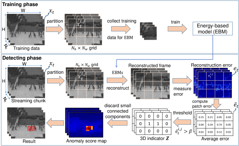
Figure 1: The overview of our proposed framework.

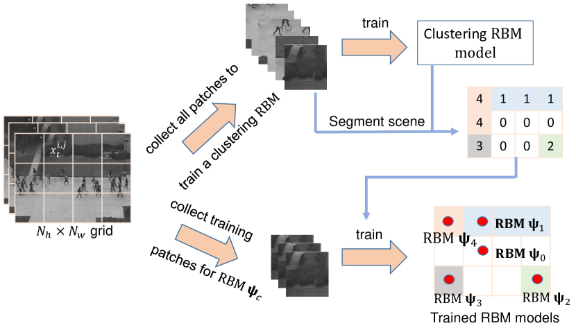
Figure 2: Scheme to train $\text{EAD }_{\text{RBM}}$ with a clustering RBM and region RBMs.

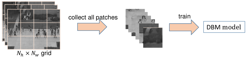
Figure 3: Scheme to train $\text{EAD }_{\text{DBM}}$ with a single DBM.

This section describes our proposed framework of Energy-based Anomaly Detection (EAD) to localize anomaly events in videos. In general, an EAD system is a two-phase pipeline of a training phase and a detection phase as demonstrated in Fig. 1. The training phase consists of three steps: (i) treating videos as a collection of images and splitting frames into a grid of patches; (ii) gathering patches and vectorizing them; (iii) training EBM models. In detection phase, the EAD system: (i) decomposes videos into patches; (ii) feeds patches into the trained EBMs for reconstructed frames and reconstruction error maps; (iii) selects regions with the high probability of being abnormal by thresholding the error maps and represents surviving regions as graphical connected components and then filters out the small anomaly objects corresponding to small-sized components; and finally (iv) updates the EBMs incrementally with video stream data. In what follows, we explain these phases in more details.

IV-A Training phase

Suppose that we denote a video of $N_{f}$ frames as $D=\{\boldsymbol{v}_{t}\in\mathbb{R}^{H\times W}\}_{t=1}^{N_{f}}$, where $H$ and $W$ are the frame size in pixel. Theoretically, we can vectorize the video frames and train the models on data vectors of $H\times W$ dimensions. However, $H\times W$ is extremely large in real-life videos, e.g., hundreds of thousand pixels, and hence it is infeasible to train EBMs in high-dimensional image space. This is because the high-dimensional input requires more complex models with an extremely large number of parameters (i.e., millions). This makes the parameter learning more difficult and less robust since it is hard to control the bounding of hidden activation values. Thus the hidden posteriors are easily collapsed into either zeros or ones, and no more learning occurs.

Another solution is to do dimensionality reduction, which projects the frames in the high dimensional input space into a subspace with lesser dimensions. But employing this solution agrees a sacrifice in terms of losing rich source of information in original images. To preserve the full information as well as reduce the data dimensionality, we choose to apply EBMs to image patches instead of the whole frames. In other words, we divide every frame $\boldsymbol{v}_{t}$ into a grid of $N_{h}\times N_{w}$ patches $\boldsymbol{v}_{t}=\{\boldsymbol{v}_{t}^{i,j}\mid 1\leq i\leq N_{h},1\leq j\leq N_{w}\}$ using the patch size of $h\times w$. These patches are flattened into vectors and gathered into a data collection to train models.

RBM-based framework

Once patch data is available, we have two possible ways to train the models: a) learn one individual RBM on patches at the same location ($i,j$) or b) learn only one RBM on all patches in the videos. The first choice results in the excessive number of models, e.g., approximate $400$ models to work on the $240\times 360$ video resolution and the non-overlapping patch size of $12\times 18$ pixels, rendering very high computational complexity and memory demand. Meanwhile, the single model approach ignores the location information of events in videos. An example is the video scene of vehicles on a street and pedestrians on a footpath. Such model cannot recognize the emergency cases when a car mounts the footpath or people suddenly cross the street without zebra-crossings.

Our solution is to reduce the number of models and preserve the location infomration by grouping similar patches at some locations and training one model for each group. This proposal is based on our observation that image patches of the same terrains, buildings or background regions (e.g., pathways, grass, streets, walls, sky or water) usually share the same appearance and texture. Therefore, using many models to represent the similar patches is redundant and they can be replaced by one shared model. To that end, we firstly cluster the video scene into similar regions by training a RBM with a few hidden units (i.e., $K=4$) on all patches. To assign a cluster to a patch $\boldsymbol{v}_{t}^{i,j}$, we compute the hidden representation $\mathrm{\boldsymbol{h}}_{r}$ of the patch and binarize it to obtain the binary vector $\tilde{\boldsymbol{h}}=\left[\mathbb{I}\left(\tilde{h}_{1}>0.5\right),...,\mathbb{I}\left(\tilde{h}_{K}>0.5\right)\right]$ where $\mathbb{I}\left(\cdot\right)$ is the indicator function. The cluster label of $\boldsymbol{v}_{t}^{i,j}$ is the decimal value of the binary vector, e.g., 0101 converted to 5. Afterwards, we compute the region label $c^{i,j}$ at location ($i,j$) by voting the labels of patches at ($i,j$) over the video frames. As a result, the similar regions of the same footpaths, walls or streets are assigned to the same label numbers and the video scene is segmented into $C$ similar regions. For each region $c$, we train a RBM parameter set $\boldsymbol{\boldsymbol{\Psi}}_{c}$ on all patches belonging to the region. After training phase, we comes up with an $\text{EAD }_{\text{RBM}}$ system with one clustering RBM and $C$ region RBMs. Fig. 2 summarizes the training procedure of our $\text{EAD }_{\text{RBM}}$.

DBM-based framework

Although $\text{EAD }_{\text{RBM}}$ can reduce the number of models dramatically, $\text{EAD }_{\text{RBM}}$ requires to train $C+1$ models, e.g., $C=16$ if $K=4$. This training procedure (Fig. 2) is still complicated. Further improvement can be done by extending the $\text{EAD }_{\text{RBM}}$ using DBMs whose multilayer structure offers more powerful capacity than the shallow structure of RBMs. In particular, one hidden layer in RBMs offers either clustering or reconstruction capacity per network whilst the multilayer networks of DBMs allow to perform multitasking in the same structure. In this work, we propose to integrate a DBM as demonstrated in Fig. 3 into EAD to detect abnormality. This network consists of two hidden layers $\mathrm{\boldsymbol{h}}^{\left(1\right)}$ and $\mathrm{\boldsymbol{h}}^{\left(2\right)}$ and two visible layers $\boldsymbol{v}^{\left(1\right)}$ and $\boldsymbol{v}^{\left(2\right)}$ at its ends. The data is always fed into both $\boldsymbol{v}^{\left(1\right)}$ and $\boldsymbol{v}^{\left(2\right)}$ simultaneously. The first hidden layer has $K$ units and it has responsibility to do a clustering task. Meanwhile, the second hidden layer has a lot of units to obtain good reconstruction capacity. These layers directly communicate with data to guarantee that the learned model can produce good examplars and reconstruction of the data. Using the proposed architecture, one DBM has the equivalent power to $C+1$ RBMs in $\text{EAD }_{\text{RBM}}$ system. Therefore, it is an appealing alternative to both clustering RBM and region RBMs in $\text{EAD }_{\text{RBM}}$. Furthermore, we only need to train one DBM, rendering a significant improvement in the number of trained models.

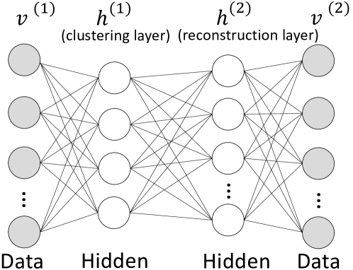
Figure 4: The architecture of our clustering and reconstruction DBM.

To train this DBM, we employ the PCD procedure, the variational approximation and the layer-wise pretraining step as described in Sec. III-B using the equations in Table IV-A. In addition, to improve the reconstruction quality of the trained model, we use conditional probabilities (Eqs. 27-30 in Table IV-A) as states of units rather than sampling them from these probabilities. This ensures to diversify the states of neurons and strengthen the reconstruction capacity of the network. But it is noteworthy that an exception is units on the first hidden layer $\mathrm{\boldsymbol{h}}^{\left(1\right)}$ whose states are still binary. This is because $\mathrm{\boldsymbol{h}}^{\left(1\right)}$ has responsibility to represent data clusters and therefore it should have limited states. A DBM’s variant that is close to our architecture is Multimodal DBMs [43]. In that study, the different types of data, e.g., images and texts, are attached into two ends of the network in order to model the joint representation across data types. By contrast, our architecture is designed to do multitasks. To the best of our knowledge, our proposed network of both reconstruction and clustering capacities is distinct from other DBM’s studies in the literature.

Energy function: $\displaystyle E\left(\boldsymbol{v},\mathrm{\boldsymbol{h}};\boldsymbol{\boldsymbol{\Psi}}\right)$ $\displaystyle=$ $\displaystyle-\mathrm{\boldsymbol{a}}^{\left(1\right)\top}\boldsymbol{v}^{\left(1\right)}-\mathrm{\boldsymbol{a}}^{\left(2\right)\top}\boldsymbol{v}^{\left(2\right)}-\mathrm{\boldsymbol{b}}^{\left(1\right)\top}\mathrm{\boldsymbol{h}}^{\left(1\right)}-\mathrm{\boldsymbol{b}}^{\left(2\right)\top}\mathrm{\boldsymbol{h}}^{\left(2\right)}$ (21) $\displaystyle-\boldsymbol{v}^{\left(1\right)\top}\boldsymbol{W}^{\left(1\right)}\mathrm{\boldsymbol{h}}^{\left(1\right)}-\mathrm{\boldsymbol{h}}^{\left(1\right)\top}\boldsymbol{W}^{\left(2\right)}\mathrm{\boldsymbol{h}}^{\left(2\right)}-\mathrm{\boldsymbol{h}}^{\left(2\right)\top}\boldsymbol{W}^{\left(3\right)}\boldsymbol{v}^{\left(2\right)}$	Parameter update equations: $\displaystyle\Delta a_{m}^{\left(l\right)}$ $\displaystyle=$ $\displaystyle\eta\left(\sum_{i=1}^{N_{s}}\frac{v_{m}^{\left(l\right)\left[i\right]}}{N_{s}}-\sum_{i=1}^{N_{\text{c}}}\frac{\hat{v}_{m}^{\left(l\right)\left\langle i\right\rangle}}{N_{\text{c}}}\right)$ (22) $\displaystyle\Delta b_{n}^{\left(l\right)}$ $\displaystyle=$ $\displaystyle\eta\left(\sum_{i=1}^{N_{s}}\frac{\tilde{\mu}_{n}^{\left(l\right)\left[i\right]}}{N_{s}}-\sum_{i=1}^{N_{\text{c}}}\frac{\hat{h}_{n}^{\left(l\right)\left\langle i\right\rangle}}{N_{\text{c}}}\right)$ (23) $\displaystyle\Delta w_{mn}^{\left(1\right)}$ $\displaystyle=$ $\displaystyle\eta\left(\sum_{i=1}^{N_{s}}\frac{v_{m}^{\left(1\right)\left[i\right]}\tilde{\mu}_{n}^{\left(1\right)\left[i\right]}}{N_{s}}-\sum_{i=1}^{N_{\text{c}}}\frac{\hat{v}_{m}^{\left(1\right)\left\langle i\right\rangle}\hat{h}_{n}^{\left(1\right)\left\langle i\right\rangle}}{N_{\text{c}}}\right)$ (24) $\displaystyle\Delta w_{mn}^{\left(2\right)}$ $\displaystyle=$ $\displaystyle\eta\left(\sum_{i=1}^{N_{s}}\frac{\tilde{\mu}_{m}^{\left(1\right)\left[i\right]}\tilde{\mu}_{n}^{\left(2\right)\left[i\right]}}{N_{s}}-\sum_{i=1}^{N_{\text{c}}}\frac{\hat{h}_{m}^{\left(1\right)\left\langle i\right\rangle}\hat{h}_{n}^{\left(2\right)\left\langle i\right\rangle}}{N_{\text{c}}}\right)$ (25) $\displaystyle\Delta w_{nm}^{\left(3\right)}$ $\displaystyle=$ $\displaystyle\eta\left(\sum_{i=1}^{N_{s}}\frac{\tilde{\mu}_{n}^{\left(2\right)\left[i\right]}v_{m}^{\left(2\right)\left[i\right]}}{N_{s}}-\sum_{i=1}^{N_{\text{c}}}\frac{\hat{h}_{n}^{\left(2\right)\left\langle i\right\rangle}\hat{v}_{m}^{\left(2\right)\left\langle i\right\rangle}}{N_{\text{c}}}\right)$ (26)
Conditional probabilities: $\displaystyle p\left(v_{m}^{\left(1\right)}=1|\mathrm{\boldsymbol{h}}^{\left(1\right)};\boldsymbol{\boldsymbol{\Psi}}\right)\text{\,\,\,\,\,\,\,\,\,\,\,\,\,}$ $\displaystyle=$ $\displaystyle\sigma\left(a_{m}^{\left(1\right)}+\boldsymbol{w}_{m\cdot}^{\left(1\right)}\mathrm{\boldsymbol{h}}^{\left(1\right)}\right)$ (27) $\displaystyle p\left(h_{n}^{\left(1\right)}=1|\boldsymbol{v}^{\left(1\right)},\mathrm{\boldsymbol{h}}^{\left(2\right)};\boldsymbol{\boldsymbol{\Psi}}\right)$ $\displaystyle=$ $\displaystyle\sigma\left(\mathrm{b}_{n}^{\left(1\right)}+\boldsymbol{v}^{\left(1\right)\top}\boldsymbol{w}_{\cdot n}^{\left(1\right)}+\boldsymbol{w}_{n\cdot}^{\left(2\right)}\mathrm{\boldsymbol{h}}^{\left(2\right)}\right)$ (28) $\displaystyle p\left(h_{n}^{\left(2\right)}=1|\mathrm{\boldsymbol{h}}^{\left(1\right)},\boldsymbol{v}^{\left(2\right)};\boldsymbol{\boldsymbol{\Psi}}\right)$ $\displaystyle=$ $\displaystyle\sigma\left(\mathrm{b}_{n}^{\left(2\right)}+\mathrm{\boldsymbol{h}}^{\left(1\right)\top}\boldsymbol{w}_{\cdot n}^{\left(2\right)}+\boldsymbol{w}_{n\cdot}^{\left(3\right)}\boldsymbol{v}^{\left(2\right)}\right)$ (29) $\displaystyle p\left(v_{m}^{\left(2\right)}=1|\mathrm{\boldsymbol{h}}^{\left(2\right)};\boldsymbol{\boldsymbol{\Psi}}\right)\text{\,\,\,\,\,\,\,\,\,\,\, }$ $\displaystyle=$ $\displaystyle\sigma\left(a_{m}^{\left(2\right)}+\mathrm{\boldsymbol{h}}^{\left(2\right)\top}\boldsymbol{w}_{\cdot m}^{\left(3\right)}\right)$ (30)
Mean-field update equations: $\displaystyle\tilde{\mu}_{n}^{\left(1\right)}$ $\displaystyle=$ $\displaystyle\sigma\left(\mathrm{b}_{n}^{\left(1\right)}+\boldsymbol{v}^{\left(1\right)\top}\boldsymbol{w}_{\cdot n}^{\left(1\right)}+\boldsymbol{w}_{n\cdot}^{\left(2\right)}\boldsymbol{\tilde{\mu}}^{\left(2\right)}\right)$ (31) $\displaystyle\tilde{\mu}_{n}^{\left(2\right)}$ $\displaystyle=$ $\displaystyle\sigma\left(\mathrm{b}_{n}^{\left(2\right)}+\boldsymbol{\tilde{\mu}}^{\left(1\right)\top}\boldsymbol{w}_{\cdot n}^{\left(2\right)}+\boldsymbol{w}_{n\cdot}^{\left(3\right)}\boldsymbol{v}^{\left(2\right)}\right)$ (32)

Table I: Equations of a clustering reconstruction DBM.

IV-B Detection phase

Once $\text{EAD }_{\text{RBM}}$ or $\text{EAD }_{\text{DBM}}$ has been learned from training data, we can use it to detect anomalous events in testing videos. The Alg. 1 shows the pseudocode of this phase that can be summarized into three main steps of: a) reconstructing frames and computing reconstruction errors; b) localizing the anomaly events and c) updating the EBMs incrementally. In what follows, we introduce these steps in more details.

1: Chunk $\left\{\boldsymbol{v}_{t}\right\}_{t=1}^{L}$, models $\boldsymbol{\boldsymbol{\Psi}}$, thresholds $\beta$ and $\gamma$

2:Detection $\boldsymbol{Z}$, score $\left\{\bar{e}_{t}^{i,j}\right\}$

3:for $t\leftarrow 1,\ldots,L$ do

4:    for $\boldsymbol{v}_{t}^{i,j}\in\boldsymbol{v}_{t}$ do

5:         $\boldsymbol{v}_{\text{r},t}^{i,j}\leftarrow$reconstruct($\boldsymbol{v}_{t}^{i,j}$,$\boldsymbol{\boldsymbol{\Psi}}$)

6:         $\boldsymbol{e}_{t}^{i,j}\leftarrow|\boldsymbol{v}_{t}^{i,j}-\boldsymbol{v}_{\text{r},t}^{i,j}|$

7:         $\bar{e}_{t}^{i,j}\leftarrow\frac{1}{h\times w}\left\|\boldsymbol{e}_{t}^{i,j}\right\|_{2}$

8:         if $\bar{e}_{t}^{i,j}\geq\beta$ then

9:             for $p\in\boldsymbol{v}_{t}^{i,j}$ do

10:                 $\boldsymbol{Z}(p)\leftarrow 1$

11:             end for

12:         else

13:             for $p\in\boldsymbol{v}_{t}^{i,j}$ do

14:                 $\boldsymbol{Z}(p)\leftarrow 0$

15:             end for

16:         end if

17:    end for

18:    //Online version only

19:    for $c\leftarrow 1,\ldots,C$ do

20:         $\boldsymbol{X}_{t}^{c}\leftarrow\left\{\boldsymbol{v}_{t}^{i,j}\mid c^{i,j}=c\right\}$

21:         $\boldsymbol{\boldsymbol{\Psi}}_{c}\leftarrow\text{{updateRBM}}(\boldsymbol{X}_{t}^{c},\boldsymbol{\boldsymbol{\Psi}})$

22:    end for

23:end for

24:$\boldsymbol{Z}\leftarrow$remove_small_components($\boldsymbol{Z},$$\gamma$)

Algorithm 1 Detection with EAD

At first, the video stream is split into chunks of $L$ non-overlapping frames $\left\{\boldsymbol{v}_{t}\right\}_{t=1}^{L}$ which next are partitioned into patches $\boldsymbol{v}_{t}^{i,j}$ as the training phase. By feeding these patches into the learned EADs, we obtain the reconstructed patches $\boldsymbol{v}_{\text{r,}t}^{i,j}$ and the reconstruction errors $\boldsymbol{e}_{t}^{i,j}=|\boldsymbol{v}_{t}^{i,j}-\boldsymbol{v}_{\text{r},t}^{i,j}|$. One can use these errors to identify anomaly pixels by comparing them with a given threshold. However, these pixel-level reconstruction errors are not reliable enough because they are sensitive to noise. As a result, this approach may produce many false alarms when normal pixels are reconstructed with high errors, and may fail to cover the entire abnormal objects in such a case that they are fragmented into isolated high error parts. Our solution is to use the patch average error $\bar{e}_{t}^{i,j}=||\boldsymbol{e}_{t}^{i,j}||_{2}/\left(h\times w\right)$ rather than the pixel errors. If $\bar{e}_{t}^{i,j}\geq\beta$, all pixels in the corresponding patch are assigned to be abnormal.

After abnormal pixels in patches are detected in each frame, we concatenate $L$ contiguous detection maps to obtain a 3D binary hyperrectangle $\boldsymbol{Z}\in\left\{0,1\right\}^{L\times H\times W}$ wherein $z_{i,j,k}=1$ indicates an abnormal voxel and otherwise $0$ is a normal one. Throughout the experiments, we observe that although most of the abnormal voxels in $\boldsymbol{Z}$ are correct, there are a few groups of abnormal voxels that are false detections because of noise. To filter out these voxels, we firstly build a sparse graph whose vertices are abnormal voxels $z_{i,j,k}=1$ and edges are connections between two vertices $z_{i,j,k}$ and $z_{i+m,j+n,k+t}$ satisfying $m,n,t\in\left\{-1,0,1\right\}$ and $\left|m\right|+\left|n\right|+\left|t\right|>0$. Then, we apply a connected component algorithm to this graph and remove noisy components that are defined to span less than $\gamma$ contiguous frames. The average errors $\bar{e}_{t}^{i,j}$ after this component filtering step can be used as a final anomaly score.

One problem is that objects can appear at different sizes and scales in videos. To tackle this problem, we independently employ the detection procedure above in the same videos at different scales. This would help the patch partially or entirely cover objects at certain scales. In particular, we rescale the original video into different resolutions, and then compute the corresponding final anomaly maps and the binary 3D indicator tensors $\boldsymbol{Z}$. The final anomaly maps at these scales are aggregated into one map using a max-operation in $\text{EAD }_{\text{RBM}}$ and a mean-operation in $\text{EAD }_{\text{DBM}}$. The mean-operation is used in $\text{EAD }_{\text{DBM}}$ is because we observe that DBMs at the finer resolutions usually cover more patches and they tend to over-detect whilst models at the coarser resolutions prefer under-detecting. Averaging maps at different scales can address these issues and produce better results. For $\text{EAD }_{\text{RBM}}$, since region RBMs frequently work in image segments and are rarely affected by scales, we can pick up the best maps over resolution. Likewise, the binary indicator tensors $\boldsymbol{Z}$ are also combined into one tensor using a binary OR-operation before proceeding the connected component filtering step. In this work, we use overlapping patches for better detection accuracy. The pixels in overlapping regions are averaged when combining maps and indicator tensors at different scales.

Incremental detection

In the scenario of data streaming where videos come on frame by frame, the scene frequently changes over time and the current frame is significantly different from those are used to train models. As a result, the models become out of date and consider all regions as abnormalities. To handle this problem, we let the models be updated with new frames. More specifically, for every oncoming frame $t$, we use all patches with region label $c$ to update the RBM $\boldsymbol{\boldsymbol{\Psi}}_{c}$ in $\text{EAD }_{\text{RBM}}$. The updating procedure is exactly the same as parameter updates (Eqs. 8-10) in training phase using gradient ascent and $20$ epochs. Here we use several epochs to ensure that the information of new data are sufficiently captured by the models.

1: Training data $\mathcal{D}=\left\{\boldsymbol{v}^{\left[i\right]}\right\}_{i=1}^{N}$, original RBM of $M$ visible and $K$ hidden units and weights $\boldsymbol{W}$, # selected hidden units $K^{\prime}$

2:New RBM with weights $\boldsymbol{W}^{\prime}$

3:for $i\leftarrow 1,\ldots,N$ do

4:    for $n\leftarrow 1,\ldots,K$ do

5:         $\tilde{h}_{n}^{\left[i\right]}\leftarrow p\left(h_{n}=1\mid\boldsymbol{v}^{\left[i\right]}\right)$

6:    end for

7:end for

8:for $n\leftarrow 1,\ldots,K$ do

9:    $\alpha_{n}\leftarrow\sum_{i=1}^{N}\sum_{m=1}^{M}\frac{\left|w_{mn}\tilde{h}_{n}^{\left[i\right]}\right|}{NM}$

10:end for

11:$j_{1},...,j_{K^{\prime}}\leftarrow\text{index\_of\_top\_max\_of}{\left[\alpha_{n}\right]}$

12:$\boldsymbol{W}^{\prime}\leftarrow\left[\mathbf{w}_{\cdot j_{1}},...,\mathbf{w}_{\cdot j_{K^{\prime}}}\right]$

Algorithm 2 Reduce RBM hidden units

For $\text{EAD }_{\text{DBM}}$, updating one DBM model for the whole scene is ineffective. The reason is that, in a streaming scenario, a good online system should have a capacity of efficiently adapting itself to the rapid changes of scenes using limited data of the current frames. These changes, e.g., new pedestrians, occur gradually in some image patches among a large number of static background patches, e.g., footpaths or grass. However, since a single DBM has to cover the whole scene, it is usually distracted by these background patches during its updating and becomes insensitive to such local changes. As a result, there is an insufficient difference in detection quality between updated and non-updated DBM models. Our solution is to build region DBMs, each of which has responsibility for monitoring patches in the corresponding region. Because each DBM observes a smaller area, it can instantly recognize the changes in that area. These region DBMs can be initialized by cloning the parameters of the trained single DBM. Nevertheless, we observe that since the clustering layer is not needed during the detection phase, we propose to remove the first visible layer $\boldsymbol{v}^{\left(1\right)}$ and the first hidden layer $\mathrm{\boldsymbol{h}}^{\left(1\right)}$, converting a region DBM to a RBM. This conversion helps $\text{EAD }_{\text{DBM}}$ perform more efficiently because updating the shallow networks of RBM with $\text{CD}{}_{1}$ is much faster than updating DBMs with Gibbs sampling and mean-field.

Overall, the streaming version of $\text{EAD }_{\text{DBM}}$ includes the following steps of: i) using the single DBM parameters to initialize the region DBMs; ii) keeping the biases and the connection matrix of reconstruction layer $\mathrm{\boldsymbol{h}}^{\left(2\right)}$ and its corresponding visible layer $\boldsymbol{v}^{\left(2\right)}$ to form region RBMs; iii) reducing the number of hidden units to obtain smaller RBMs using Alg. 2; iv) fine-tuning the region RBMs using the corresonding patch data from the training videos; and v) applying the same procedure in $\text{EAD }_{\text{RBM}}$ to detect and update the region RBMs. The steps i-iv) are performed in the training phase as soon as the single DBM has been learned whilst the last step is triggered in the detection phase. The step iii) is introduced because the reconstruction layer in $\text{EAD }_{\text{DBM}}$ usually needs more units than the region RBMs in $\text{EAD }_{\text{RBM}}$ with the same reconstruction capacity. Therefore, we propose to decrease the number of DBM’s hidden units by discarding the units that have less contributions (low average connection strength $\alpha_{n}$ in the line 7 of Alg. 2) to reconstruct the data before using the training set to fine-tune these new RBMs.

V Experiment

In this section, we investigate the performance of our proposed EAD, wherein we demonstrate the capacity of capturing data regularity, reconstructing scenes and detecting anomaly events. We provide a quantitative comparison with state-of-the-art unsupervised anomaly detection systems. In addition, we introduce some potential applications of our methods for video analysis and scene clustering.

Figure 5: Clustering results of the clustering $\text{EAD }_{\text{RBM}}$, $\text{EAD }_{\text{DBM-200}}$ and k-means in UCSD Ped 1, Ped 2 and Avenue datasets.

The experiments are conducted on 3 benchmark datasets: UCSD Ped 1, Ped 2 [44] and Avenue [17]. Since these videos are provided at different resolutions, we resize all of them into the same frame size of $240\times 360$. Following the unsupervised learning setting, we discard all label information in the training set before fitting the models. All methods are evaluated on the testing videos using AUC (area under ROC curve) and EER (equal error rate) at frame-level [44], pixel-level [44] and dual-pixel level [45]. At frame-level, the systems only focus on answering whether a frame contains any anomaly object or not. By contrast, pixel-level requires the systems to take into account the locations of anomaly objects in frames. A detection is considered to be correct if it covers at least $40\%$ of anomaly pixels in the ground-truth. However, the pixel-level evaluation can be easily fooled by assigning anomalous labels to every pixels in the scene. Dual-pixel level tackles this issue by adding one constraint of at least $\alpha$ percent of decision being true anomaly pixels. It can be seen that pixel-level is a special case of the dual-pixel level when $\alpha=0$.

To deal with the changes of objects in size and scale, we process video frames at the scale ratios of $1.0$, $0.5$ and $0.25$ which indicate no, a half and a quarter reduction in each image dimension. We set the patch size to $12\times 18$ pixels and patch strides to $6$ and $9$ pixels in vertical and horizontal directions respectively. For $\text{EAD }_{\text{RBM}}$, we use a clustering RBM with 4 hidden units and region RBMs with $100$ hidden units. All of them are trained using $\text{CD}_{1}$ with $500$ epochs and a learning rate $\eta=0.1$. For $\beta$ and $\gamma$, we tune these hyperparameters to achieve the best balanced AUC and EER scores and come up with $\beta$ = 0.0035 and $\gamma=10$. For $\text{EAD }_{\text{DBM}}$ system, a DBM with 4 hidden units in the clustering layer and $200$ hidden units in reconstruction layer (Fig. 4) is investigated. In fact, we also test a DBM network with $\mathrm{\boldsymbol{h}}^{\left(1\right)}$ of 4 units and $\mathrm{\boldsymbol{h}}^{\left(2\right)}$of $100$ units. However, since there exists correlations between these hidden layers, $100$ hidden units in DBM cannot produce similar reconstruction quality to $100$ hidden units in region RBMs (Fig. 6) and therefore, more reconstruction units are needed in DBMs. As a result, we use DBM with 200 reconstruction units in all our experiments. We train DBMs using PCD [41] with $500$ epochs, pretraining procedure in [6] with $50$ epochs and a smaller learning rate of $0.001$. Two thresholds are $\beta=0.0043$ and $\gamma=10$. For the streaming versions of $\text{EAD }_{\text{RBM}}$ and $\text{EAD }_{\text{DBM}}$ (we name them $\text{EAD }_{\text{S-RBM}}$ and $\text{EAD }_{\text{S-DBM}}$), we split videos into non-overlapping chunks of $L=20$ contiguous frames. After every frame, the systems update their parameters using gradient ascent procedure in $20$ epochs. The thresholds $\beta$ and $\gamma$ are set to $0.003$ and $10$ respectively. All experiments are conducted on a Linux server with 32 CPUs of 3 GHz and 126 GB RAM.

Figure 6: Reconstruction quality of $\text{EAD }_{\text{DBM-100}}$, $\text{EAD }_{\text{DBM-200}}$ and $\text{EAD }_{\text{RBM}}$. $\text{EAD }_{\text{DBM-200}}$ has equivalent reconstruction quality to $\text{EAD }_{\text{RBM}}$ whilst $\text{EAD }_{\text{DBM-100}}$ produces unclear image (e.g., the cyclist on the left of the scene).

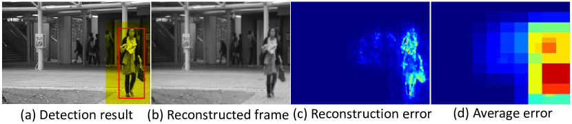
Figure 7: Data reconstruction produced by $\text{EAD }_{\text{S-DBM}}$ on Avenue dataset: (a) the original frame with a yellow region of detected outlier female and a red rectangle of ground-truth, (b) reconstructed frame, (c) reconstruction error image, (d) average reconstruction errors of patches.

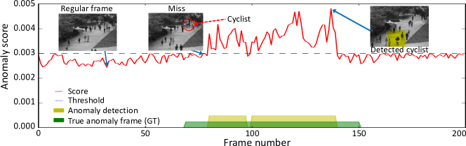
Figure 8: Average reconstruction error per frame in test video #1 of UCSD Ped 1 dataset. The shaded green region illustrates anomalous frames in the ground truth, while the yellow anomalous frames detected by $\text{EAD }_{\text{S-DBM}}$. The blue line shows the threshold.

V-A Scene clustering

In the first experiment, we investigate the performance of clustering modules in the proposed systems. More specifically, a clustering RBM network of $4$ hidden units has a responsibility to do the clustering task in $\text{EAD }_{\text{RBM}}$ while the first hidden layer of $4$ units is used to do this step in $\text{EAD }_{\text{DBM}}$. The clustering results are shown in Fig. 5. Overall, both $\text{EAD }_{\text{RBM}}$ and $\text{EAD }_{\text{DBM}}$ discover plausible clustering maps of similar quality. Using $4$ binary units, we expect that the systems can group video scenes into maximum $2^{4}=16$ groups but interestingly, they use less and return varied number of clusters depending on the video scenes and scales. For examples, $\text{EAD }_{\text{RBM}}$ uses ($6$, $7$, $10$) clusters for three scales ($1.0$, $0.5$, $0.25$) respectively in Ped 1 dataset whilst the numbers are ($9$, $9$, $8$) and ($6$, $9$, $9$) in Ped 2 and Avenue datasets. Similarly, we observe the triples produced by $\text{EAD }_{\text{DBM}}$ are ($9$, $9$, $11$) in Ped 1, ($7$, $9$, $6$) in Ped 2 and ($9$, $9$, $8$) in Avenue. The capacity of automatically selecting the appropriate number of groups shows how well our EADs can understand the scene and its structure.

For further comparison, we deploy $k$-means with $k=8$ clusters, the average number of clusters of $\text{EAD }_{\text{RBM}}$ and $\text{EAD }_{\text{DBM}}$ described above. The clustering maps in the last column of Fig. 5 show $k$-means fails to recognize large homogeneous regions, resulting in fragmenting them into many smaller regions. This is due to the impact of surrounding objects and complicated events in reality such as the shadow of the trees (case 1 in the figure) or the dynamics of crowded areas in the upper side of the footpath (case 2). In addition, $k$-means tends to produce many spots with wrong labels inside large clusters as shown in case 3. By contrast, two energy-based systems consider the factor of uncertainty and therefore are more robust to these randomly environmental factors.

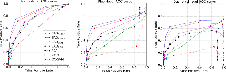
Figure 9: Comparison ROC curves on UCSD Ped 2. Three figures share the same legend. Higher curves indicate better performance. It is notable that, unlike frame and pixel-level evaluations, dual-pixel level curves may end at any points lower than (1,1).

	Ped 1					Ped 2					Avenue
	Frame		Pixel		Dual	Frame		Pixel		Dual	Frame		Pixel		Dual
	AUC	EER	AUC	EER	AUC	AUC	EER	AUC	EER	AUC	AUC	EER	AUC	EER	AUC
Unsupervised methods
PCA [20]	60.28	43.18	25.39	39.56	8.76	73.98	29.20	55.83	24.88	44.24	74.64	30.04	52.90	37.73	43.74
OC-SVM	59.06	42.97	21.78	37.47	11.72	61.01	44.43	26.27	26.47	19.23	71.66	33.87	33.16	47.55	33.15
GMM	60.33	38.88	36.64	35.07	13.60	75.20	30.95	51.93	18.46	40.33	67.27	35.84	43.06	43.13	41.64
Deep models
CAE (FR) [32]	53.50	48.00	_	_	_	81.40	26.00	_	_	_	73.80	32.80	_	_	_
ConvAE [33]	81.00	27.90	_	_	_	90.00	21.70	_	_	_	70.20	25.10	_	_	_
Our systems
$\text{EAD }_{\text{RBM}}$	64.83	37.94	41.87	36.54	16.06	76.70	28.56	59.95	19.75	46.13	74.88	32.49	43.72	43.83	41.57
$\text{EAD }_{\text{DBM}}$(100 units)	64.33	39.42	26.96	34.93	19.24	71.63	34.38	38.82	20.50	37.65	77.40	30.96	43.86	45.21	43.15
$\text{EAD }_{\text{DBM}}$(200 units)	64.60	39.29	28.16	35.19	20.21	76.52	32.04	45.56	19.40	44.17	77.53	30.79	42.94	44.61	42.26
$\text{EAD }_{\text{S-RBM}}$	70.25	35.40	48.87	33.31	22.07	86.43	16.47	72.05	15.32	66.14	78.76	27.21	56.08	34.40	53.40
$\text{EAD }_{\text{S-DBM}}$(200 units)	68.35	36.17	43.17	34.79	20.02	83.87	19.25	68.52	17.16	62.69	77.21	28.52	52.62	36.84	51.43

Table II: Anomaly detection results (AUC and EER) at frame-level, pixel-level and dual pixel-level ($\alpha=5\%)$ on 3 datasets. Higher AUC and lower EER indicate better performance. Meanwhile, high dual-pixel values point out more accurate localization. We do not report EER for dual-pixel level because this number do not always exist. Best scores are in bold whilst the next best is underlined. Note that the frame-level results of CAE (FR) and ConvAE are taken from [32] and [33] respectively, but the pixel-level and dual-pixel level results are not available.

V-B Scene reconstruction

The key ingredient of our systems for distinguishing anomaly behaviors in videos is the capacity of reconstructing data, which directly affects detection results. In this part, we give a demonstration of the reconstruction quality of our proposed systems. Fig. 7 is an example of a video frame with an anomaly object, which is a girl moving toward the camera. Our $\text{EAD }_{\text{S-DBM}}$ produces the corresponding reconstructed frame in Fig. 7b whilst the pixel error map and the average error map are shown in Fig. 7c and 7d, respectively. It can be seen that there are many high errors in anomaly regions but low errors in the other regular areas. This confirms that our model can capture the regularity very well and recognize unusual events in frames using reconstruction errors (Fig. 7a).

To demonstrate the change of the reconstruction errors with respect to the abnormality in frame sequence, we draw the maximum average reconstruction error in a frame as a function of frame index. As shown in Fig. 8, the video #1 in UCSD Ped 1 starts with a sequence of normal pedestrians walking on a footpath, followed by an irregular cyclist moving towards the camera. Since the cyclist is too small and covered by many surrounding pedestrians in the first few frames of its emergence, its low anomaly score reveals that our system cannot distinguish it from other normal objects. However, the score increases rapidly and exceeds the threshold after several frames and the system can detect it correctly.

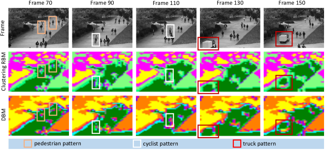
Figure 10: Some examples of pattern maps illustrate how $\text{EAD }_{\text{DBM}}$ expresses different objects at the abstract levels in a video sequence. The frames were taken from video #14, UCSD Ped 1 dataset.

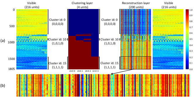
Figure 11: Activation visualization of the DBM network corresponding to 1805 patches of 5 random UCSD Ped 2 frames at scale 0.5: a) activations of the layers and their correlations; and b) a close view of reconstruction layer activations of different patches sharing the same cluster id.

V-C Anomaly detection

To evaluate our EAD systems in anomaly detection task, we compare $\text{EAD }_{\text{RBM}}$ and $\text{EAD }_{\text{DBM}}$ and our streaming versions $\text{EAD }_{\text{S-RBM}}$ and $\text{EAD }_{\text{S-DBM}}$ with several unsupervised anomaly detection systems in the literature. These systems can be categorized into a) unsupervised learning methods including Principal Component Analysis (PCA), One-Class Support Vector Machine (OC-SVM) and Gaussian Mixture Model (GMM); and b) the state-of-the-art deep models including CAE [32] and ConvAE [33].

We use the implementation of PCA with optical flow features for anomaly detection in [20]. For unsupervised baselines of OC-SVM and GMM, we use the same procedure of our $\text{EAD }_{\text{RBM}}$ framework but use $k$-means, instead of the clustering RBM, to group image patches into clusters and OC-SVM/GMM models, instead of the region RBMs, to compute the anomaly scores. Their hyperparameters are turned to gain the best cross-validation results, namely we set kernel width and lower bound of the fraction of support vectors to $0.1$ and $10^{-4}$ for OC-SVM while the number of Gaussian components and anomaly threshold in GMM are $20$ and $-50$ respectively. It is worthy to note that we do not consider the incremental versions of PCA, OC-SVM and GMM since it is not straightforward to update those models in our streaming setting. Finally, the results of competing deep learning methods are adopted from their original papers. Although CAE and ConvAE were tested on both frame data and hand-crafted features in [32, 33], we only include their experimental results on raw data for fair comparison with our models which mainly work without hand-crafted features.

	Ped 1	Ped 2	Avenue	Average
$\text{EAD }_{\text{RBM}}$	137,736	79,576	122,695	113,336
$\text{EAD }_{\text{DBM}}$	123,073	108,637	125,208	118,973

Table III: Training time of $\text{EAD }_{\text{RBM}}$ and $\text{EAD }_{\text{DBM}}$ in second.

Table II reports the experimental results of our systems versus all methods whilst Fig. 9 shows ROC curves of our methods and unsupervised learning methods. Overall, our energy-based models are superior to PCA, OC-SVM and GMM in terms of higher AUC and lower ERR. Interestingly, our higher AUCs in dual-pixel level reveals that our methods can localize anomalous regions more correctly. These results are also comparable with other state-of-the-art video anomaly detection systems using deep learning techniques (i.e., CAE [32] and ConvAE [33]). Both CAE and ConvAE are deep Autoencoder networks (12 layers) that are reinforced with the power of convolutional and pooling layers. By contrast, our systems only have a few layers and basic connections between them but obtain respectable performance. For this reason, we believe that our proposed framework of energy-based models is a promising direction to develop anomaly detection systems in future surveillance applications.

Comparing between $\text{EAD }_{\text{RBM}}$ and $\text{EAD }_{\text{DBM}}$, Table II shows that $\text{EAD }_{\text{DBM}}$ with 100 reconstruction hidden units is not so good as $\text{EAD }_{\text{RBM}}$ (with the same number of hidden units). This is because the reconstruction units in DBMs have to make additional alignment with the clustering units and therefore there is a reduction in reconstruction and detection quality. However, by adding more units to compensate for such decrease, our $\text{EAD }_{\text{DBM}}$ with 200 hidden units can obtain similar detection results to $\text{EAD }_{\text{RBM}}$. Therefore, we choose the DBM network with 200 reconstruction hidden units as the core of our $\text{EAD }_{\text{DBM}}$ system. To shorten notation, we write $\text{EAD }_{\text{DBM}}$ (without the explicit description of the number of hidden units) for a system with 200 reconstruction hidden units.

The training time of two systems is reported in Table III. Overall, there is no much different in training time between them because DBM learning procedure with expensive Gibbs sampling and mean-field steps and additional pretraining cost is more time-consuming than $\text{CD}_{1}$ in RBM training. However, one advantage of $\text{EAD }_{\text{DBM}}$ system is that it requires to train one DBM model for every video scale versus many models (i.e., 9 models in average) in $\text{EAD }_{\text{RBM}}$. Another benefit of $\text{EAD }_{\text{DBM}}$ is the capacity of model explanation, which will be discussed in the following section.

V-D Video analysis and model explanation

The clustering module in our systems is not only applied for scene segmentation but also useful for many applications such as video analysis and model explanation. Unlike other clustering algorithms that are mainly based on the common characteristics (e.g., distance, density or distribution) to group data points together, the clustering modules in EAD leverage the representation power of energy-based models (i.e. RBMs and DBMs) at abstract levels. For example, we understand that a RBM with sufficient hidden units is able to reconstruct the input data at excellent quality [46]. If we restrict it to a few hidden neurons, e.g., 4 units in our clustering RBM, the network is forced to learn how to describe the data using limited capacity, e.g., maximum 16 states for 4 hidden units, rendering the low-bit representation of the data. This low-bit representation offers an abstract and compact view of the data and therefore brings us high-level information. Fig. 10 reveals abstract views (pattern maps) of several frames from USCD Ped 1 dataset, which are exactly produced by the clustering RBM in $\text{EAD }_{\text{RBM}}$ and the clustering layer in $\text{EAD }_{\text{DBM}}$. It can be seen that different objects have different patterns. More specifically, all people can be represented as patterns of purple and lime blocks (frame 70 in Fig. 10) but their combination varies in human pose and size. The variation in the representation of people is a quintessence of articulated objects with the high levels of deformation. On the other hand, a rigid object usually has a consistent pattern, e.g., the light truck in frames 130 and 150 of Fig. 10 has a green block to describe a cargo space and smaller purple, yellow and orange blocks to represent the lower part. This demonstration shows a potential of our systems for video analysis, where the systems assist human operators by filtering out redundant information at the pixel levels and summarizing the main changes in videos at the abstract levels. The pattern maps in Fig. 10 can also be used as high level features for other computer vision systems such as object tracking, object recognition and motion detection.

The abstract representation of the videos also introduces another nice property of model explanation in our systems. Unlike most video anomaly detection systems [33, 32, 34, 31, 29, 30, 28, 27, 26] that only produce final detection results without providing any evidence of model inference, the pattern maps show how our models view the videos and therefore they are useful cues to help developers debug the models and understand how the systems work. An example is the mis-recognitions of distant cyclists to be normal objects. By examining the pattern maps of frames 90 and 110 in Fig. 10, we can easily discover that distant cyclists share the same pattern of purple and lime colors with pedestrians. Essentially, cyclists are people riding bicycles. When the bicycles are too small, they are unable to be recognized by the detectors and the cyclists are considered as pedestrians. This indicates that our pattern maps can offer a rational explanation of the system mistakes.

There unlikely exists a model explanation capacity mentioned above in $\text{EAD }_{\text{RBM}}$ because its clustering module and its reconstruction module are built separately and thus it does not ensure to obtain an alignment between abstract representation (provided by clustering RBMs) and detection decision (by region RBMs). As a result, what we see in the pattern maps may not reflect what the model actually does. By contrast, both clustering layer and reconstruction layer are trained parallelly in $\text{EAD }_{\text{DBM}}$, rendering a strong correlation between them via their weight matrix. Fig. 11 demonstrates this correlation. We firstly collect all 1805 patches at the scale 0.5 from 5 random frames of UCSD Ped 2 dataset and then feed them into the network and visualize the activation values of the layers after running the mean-field procedure. Each picture can be viewed as a matrix of (# patches) rows and (# units) columns. Each horizontal line is the response of neurons and layers to the corresponding input patch. As shown in Fig. 11a, there is a strong agreement in color between the layers, for example, the cyan lines in two visible layers always correspond to red lines in the clustering layer and yellow lines in the reconstruction layer and similarly yellow inputs are frequently related to the blue responses of the hidden neurons. We can understand this by taking a closer look at the structure of our proposed DBM. The connections with data ensure that the clustering layer and the reconstruction layer have to represent the data whilst their connections force them to align with each other. However, it is worthy to note that the reconstruction layer is not simply a copy of the clustering layer but it adds more details towards describing the corresponding data. As a result, there are still distinctions between reconstruction layer responses of two different patches with the same clustering layer responses. Imagine that we have two white patches of a footpath with and without some parts of a pedestrian. As we know in Sec. V-A, these patches are assigned to the same cluster or have the same clustering layer states that represent footpath regions. Next, these states specify the states of the reconstruction layer and make them similar. However, since these patches are different, the patch with the pedestrian slightly modifies the state of the reconstruction layer to describe the presence of the pedestrian. Fig. 11b confirms this idea. All reconstruction layer responses have the same cluster layer state of $\left(0,0,0,0\right)$, and therefore the similar horizontal color strips, but they are still different in intensity. All aforementioned discussions conclude that the clustering layer in DBM is totally reliable to reflect the operation of the system and it is useful to visualize and debug the models. It is noteworthy that this capacity is not present in shallow networks like RBMs.

VI Conclusion

This study presents a novel framework to deal with three existing problems in video anomaly detection, that are the lack of labeled training data, no explicit definition of anomaly objects and the dependence on hand-crafted features. Our solution is based on energy-based models, namely Restricted Boltzmann Machines and Deep Boltzmann Machines, that are able to learn the distribution of unlabeled raw data and then easily isolate anomaly behaviors in videos. We design our anomaly detectors as 2-module systems of a clustering RBM/layer to segment video scenes and region RBMs/reconstruction layer to represent normal image patches. Anomaly signals are computed using the reconstruction errors produced by the reconstruction module. The extensive experiments conducted in 3 benchmark datasets of UCSD Ped 1, Ped 2 and Avenue show the our proposed framework outperforms other unsupervised learning methods in this task and achieves comparable detection performance with the state-of-the-art deep detectors. Furthermore, our framework also has a lot of advantages over many existing systems, i.e. the nice capacities of scene segmentation, scene reconstruction, streaming detection, video analysis and model explanation.

Hung Vu is a PhD candidate and Postgraduate Research Scholar supported by Deakin University, Australia. He received his Bachelor and Master of Computer Science degrees from University of Sciences, HCMC, Vietnam National University (VNU), Vietnam, in 2008 and 2011. His research interests are the intersection of computer vision and machine learning. His current projects focus on deep generative networks, Boltzmann machines and their applications to anomaly detection and video surveillance.

Tu Dinh Nguyen obtained a Bachelor of Science from Vietnam National University, and a PhD in Computer Science from Deakin University in 2010 and 2015, respectively. Currently he is a Research Fellow at Deakin University, Australia. His research interests are deep generative models, kernel methods, online learning and distributed computing. He has won several research awards: Best Application Paper Award at PAKDD conference (2017), Best Runner-Up Student Paper Award at PAKDD conference (2015), and Honorable Mention Application Paper Award at DSAA conference (2017). Tu achieved the title of “Kaggle master” on July 2014.

Dinh Phung is currently a Professor and Deputy Director in the Centre for Pattern Recognition and Data Analytics within the School of Information Technology, Deakin University, Australia. He obtained a Ph.D. from Curtin University in 2005 in the area of machine learning and multimedia computing. His current research interest include machine learning, graphical models, Bayesian nonparametrics, statistical deep networks, online learning and their applications in diverse areas such as pervasive healthcare, autism and health analytics, computer vision, multimedia and social computing. He has published 180+ papers and 2 patents in the area of his research interests. He has won numerous research awards, including the Best Paper Award at PAKDD conference (2015), Best Paper Award Runner-Up at UAI conference (2009), Curtin Innovation Award from Curtin University for developing groundbreaking technology in early intervention for autism (2011), Victorian Education Award (Research Engagement 2013) and an International Research Fellowship from SRI International in 2005. His research program has regularly attracted competitive research funding from the Australian Research Council (ARC) in the last 10 years and from the industry. He has delivered several invited and keynote talks, served on 40+ organizing committees and technical program committees for topnotch conferences in machine learning and data analytics, including his recent role as the Program Co-Chair for the Asian Conference on Machine Learning in 2014.

References

- [1] A. A. Sodemann, M. P. Ross, and B. J. Borghetti, “A Review of Anomaly Detection in Automated Surveillance,” IEEE Transactions on Systems, Man, and Cybernetics, Part C (Applications and Reviews), vol. 42, pp. 1257 – 1272, November 2012.
- [2] G. Zhou and Y. Wu, “Anomalous Event Detection Based on Self-Organizing Map for Supermarket Monitoring,” in International Conference on Information Engineering and Computer Science, December 2009, pp. 1–4.
- [3] N. Dalal and B. Triggs, “Histograms of Oriented Gradients for Human Detection,” in CVPR, San Diego, CA, USA, June 20-26 2005, pp. 886–893.
- [4] N. Dalal, B. Triggs, and C. Schmid, “Human Detection Using Oriented Histograms of Flow and Appearance,” in ECCV, Berlin, Heidelberg, 2006, pp. 428–441.
- [5] B. D. Lucas and T. Kanade, “An Iterative Image Registration Technique with an Application to Stereo Vision,” in IJCAI, San Francisco, CA, USA, 1981, pp. 674–679.
- [6] R. Salakhutdinov and G. Hinton, “Deep Boltzmann Machines,” in AISTATS, vol. 5, 2009, pp. 448–455.
- [7] T. D. Nguyen, T. Tran, D. Phung, and S. Venkatesh, “Learning Parts-based Representations with Nonnegative Restricted Boltzmann Machine,” in ACML, vol. 29, Australian National University, Canberra, Australia, 13–15 November 2013, pp. 133–148.
- [8] T. Tran, T. D. Nguyen, D. Q. Phung, and S. Venkatesh, “Learning Vector Representation of Medical Objects via EMR-Driven Nonnegative restricted Boltzmann machines (eNRBM),” Journal of Biomedical Informatics, vol. 54, pp. 96–105, 2015.
- [9] T. D. Nguyen, T. Tran, D. Q. Phung, and S. Venkatesh, “Latent Patient Profile Modelling and Applications with Mixed-Variate Restricted Boltzmann Machine,” in PAKDD, vol. 7818, 2013, pp. 123–135.
- [10] H. Vu, T. D. Nguyen, A. Travers, S. Venkatesh, and D. Phung, “Energy-Based Localized Anomaly Detection in Video Surveillance,” in PAKDD, Jeju, South Korea, May 23-26 2017.
- [11] Y. Freund and D. Haussler, “Unsupervised Learning of Distributions on Binary Vectors Using Two Layer Networks,” Santa Cruz, CA, USA, Tech. Rep., 1994.
- [12] G. Hinton, “Training Products of Experts by Minimizing Contrastive Divergence,” Neural Computation, vol. 14, no. 8, pp. 1771–1800, 2002.
- [13] X. Cui, Q. Liu, M. Gao, and D. N. Metaxas, “Abnormal Detection using Interaction Energy Potentials,” in CVPR, June 2011.
- [14] D. Singh and C. K. Mohan, “Graph Formulation of Video Activities for Abnormal Activity Recognition,” Pattern Recognition, vol. 65, pp. 265–272, 2017.
- [15] I. Laptev, “On Space-Time Interest Points,” IJCV, vol. 64, no. 2, pp. 107–123, September 2005.
- [16] Y. Zhang, H. Lu, L. Zhang, and X. Ruan, “Combining Motion and Appearance Cues for Anomaly Detection,” Pattern Recognition, vol. 51, pp. 443–452, 2016.
- [17] C. Lu, J. Shi, and J. Jia, “Abnormal Event Detection at 150 FPS in MATLAB,” in ICCV, Sydney, Australia, December 2013.
- [18] Y. Fan, G. Wen, S. Qiu, and D. Li, “Detecting Anomalies in Crowded Scenes via Locality-constrained Affine Subspace Coding,” Journal of Electronic Imaging, vol. 26, pp. 26 – 26 – 9, 2017.
- [19] S. Wu, B. E. Moore, and M. Shah, “Chaotic Invariants of Lagrangian Particle Trajectories for Anomaly Detection in Crowded Scenes,” in CVPR, June 2010.
- [20] D.-S. Pham, B. Saha, D. Q. Phung, and S. Venkatesh, “Detection of Cross-channel Anomalies from Multiple Data Channels,” in ICDM, 2011, pp. 527–536.
- [21] B. Zhao, L. Fei-Fei, and E. P. Xing, “Online Detection of Unusual Events in Videos via Dynamic Sparse Coding,” in CVPR, Washington, DC, USA, 2011, pp. 3313–3320.
- [22] T. Wang, M. Qiao, A. Zhu, Y. Niu, C. Li, and H. Snoussi, “Abnormal Event Detection via Covariance Matrix for Optical Flow based Feature,” Multimedia Tools and Applications, November 2017.
- [23] M. J. Roshtkhari and M. D. Levine, “Online Dominant and Anomalous Behavior Detection in Videos,” in CVPR, Washington, DC, USA, 2013, pp. 2611–2618.
- [24] T. V. Duong, H. H. Bui, D. Q. Phung, and S. Venkatesh, “Activity Recognition and Abnormality Detection with the Switching Hidden Semi-Markov Model,” in CVPR, vol. 1, Washington, DC, USA, 2005, pp. 838–845.
- [25] Y. Guo, Y. Liu, A. Oerlemans, S. Lao, S. Wu, and M. S. Lew, “Deep Learning for Visual Understanding: A Review,” Neurocomputing, vol. 187, pp. 27 – 48, 2016.
- [26] M. Sabokrou, M. Fayyaz, M. Fathy, and R. Klette, “Deep-Anomaly: Fully Convolutional Neural Network for Fast Anomaly Detection in Crowded Scenes,” CVIU, 2018.
- [27] M. Ravanbakhsh, M. Nabi, E. Sangineto, L. Marcenaro, C. S. Regazzoni, and N. Sebe, “Abnormal Event Detection in Videos using Generative Adversarial Nets,” in ICIP, September 2017, pp. 1577–1581.
- [28] H. Tran and D. Hogg, “Anomaly Detection using a Convolutional Winner-Take-All Autoencoder,” in BMVC, London, September 2017.
- [29] Y. S. Chong and Y. H. Tay, “Abnormal Event Detection in Videos Using Spatiotemporal Autoencoder,” in International Symposium on Neural Networks, Japan, June 21–26 2017, pp. 189–196.
- [30] W. Luo, W. Liu, and S. Gao, “Remembering History with Convolutional LSTM for Anomaly Detection,” in ICME, July 2017, pp. 439–444.
- [31] J. R. Medel and A. E. Savakis, “Anomaly Detection in Video Using Predictive Convolutional Long Short-Term Memory Networks,” CoRR, 2016.
- [32] M. Ribeiro, A. E. Lazzaretti, and H. S. Lopes, “A Study of Deep Convolutional Auto-Encoders for Anomaly Detection in Videos,” Pattern Recognition Letters, 2017.
- [33] M. Hasan, J. Choi, J. Neumann, A. K. Roy-Chowdhury, and L. S. Davis, “Learning Temporal Regularity in Video Sequences,” in CVPR, 2016.
- [34] D. Xu, Y. Yan, E. Ricci, and N. Sebe, “Detecting Anomalous Events in Videos by Learning Deep Representations of Appearance and Motion,” CVIU, vol. 156, pp. 117–127, 2017.
- [35] K. Do, T. Tran, D. Phung, and S. Venkatesh, “Outlier Detection on Mixed-Type Data: An Energy-Based Approach,” in Proceedings in the 12th International Conference on Advanced Data Mining and Applications (ADMA), Gold Coast, Queensland, Australia, December 12-15 2016, pp. 111–125.
- [36] S. Zhai, Y. Cheng, W. Lu, and Z. Zhang, “Deep Structured Energy Based Models for Anomaly Detection,” in ICML, vol. 48, New York, New York, USA, June 20–22 2016, pp. 1100–1109.
- [37] A. Hyvärinen, “Estimation of Non-Normalized Statistical Models by Score Matching,” JMLR, vol. 6, pp. 695–709, December 2005.
- [38] P. Vincent, “A Connection Between Score Matching and Denoising Autoencoders,” Neural Computation, vol. 23, no. 7, pp. 1661–1674, 2011.
- [39] A. R. Revathi and D. Kumar, “An Efficient System for Anomaly Detection using Deep Learning Classifier,” in Signal, Image and Video Processing, August 2016.
- [40] R. Salakhutdinov and G. Hinton, “An Efficient Learning Procedure for Deep Boltzmann Machines,” Neural Computation, vol. 24, no. 8, pp. 1967–2006, August 2012.
- [41] T. Tieleman, “Training Restricted Boltzmann Machines Using Approximations to the Likelihood Gradient,” in ICML, New York, NY, USA, 2008, pp. 1064–1071.
- [42] M. A. Carreira-Perpinan and G. E. Hinton, “On Contrastive Divergence Learning,” in Intelligence, Artificial and Statistics, Barbados, 2005.
- [43] N. Srivastava and R. Salakhutdinov, “Multimodal learning with deep boltzmann machines,” JMLR, vol. 15, pp. 2949–2980, 2014.
- [44] W.-X. Li, V. Mahadevan, and N. Vasconcelos, “Anomaly Detection and Localization in Crowded Scenes,” in TPAMI, vol. 36, no. 1, 2014, pp. 18–32.
- [45] M. Sabokrou, M. Fathy, M. Hosseini, and R. Klette, “Real-Time Anomaly Detection and Localization in Crowded Scenes,” CVPRW, 2015.
- [46] N. Le Roux and Y. Bengio, “Representational Power of Restricted Boltzmann Machines and Deep Belief Networks,” Neural Computation, vol. 20, no. 6, pp. 1631–1649, 2008.