A new analysis of Work Stealing with latency

Abstract.

We study in this paper the impact of communication latency on the classical Work Stealing load balancing algorithm. Our paper extends the reference model in which we introduce a latency parameter. By using a theoretical analysis and simulation, we study the overall impact of this latency on the Makespan (maximum completion time). We derive a new expression of the expected running time of a bag of tasks scheduled by Work Stealing. This expression enables us to predict under which conditions a given run will yield acceptable performance. For instance, we can easily calibrate the maximal number of processors to use for a given work/platform combination. All our results are validated through simulation on a wide range of parameters.

1. Introduction

The motivation of this work is to study how to extend the analysis of the Work Stealing (WS) algorithm in a distributed-memory context, where communications matter. WS is a classical on-line scheduling algorithm proposed for shared-memory multi-cores (Arora et al., 2001) whose principle is recalled in the next section. As it is common, we target the minimization of the Makespan, defined as the maximum completion time of the parallel application. We present a theoretical analysis for an upper bound of the expected makespan and we run a complementary series of simulations in order to assess how this new bound behaves in practice depending on the value of the latency.

1.1. Motivation for studying WS with latency

Distributed-memory clusters consist in independent processing elements with private local memories linked by an interconnection network. In such architectures, communication issues are crucial, they highly influence the performances of the applications (Hamid et al., 2015b). However, there are only few works dealing with optimized allocation strategies and the relationships with the allocation and scheduling process is most often ignored. In practice, the impact of scheduling may be huge since the whole execution can be highly affected by a large communication latency of interconnection networks (Hamid et al., 2015a). Scheduling is the process which aims at determining where and when to execute the tasks of a target parallel application. The applications are represented as directed acyclic graphs where the vertices are the basic operations and the arcs are the dependencies between the tasks (Cosnard and Trystram, 1995). Scheduling is a crucial problem which has been extensively studied under many variants for the successive generations of parallel and distributed systems. The most commonly studied objective is to minimize the makespan (denoted by $C_{\max}$) and the underlying context is usually to consider centralized algorithms. This assumption is not always realistic, especially if we consider distributed memory allocations and an on-line setting.

WS is an efficient scheduling mechanism targeting medium range parallelism of multi-cores for fine-grain tasks. Its principle is briefly recalled as follows: each processor manages its own (local) list of tasks. When a processor becomes idle it randomly chooses another processor and steals some work (if possible). Its analysis is probabilistic since the algorithm itself is randomized. Today, the research on WS is driven by the question on how to extend the analysis for the characteristics of new computing platforms (distributed memory, large scale, heterogeneity). Notice that beside its theoretical interest, WS has been implemented successfully in several languages and parallel libraries including Cilk (Frigo et al., 1998; Leiserson, 2009), TBB (Threading Building Blocks) (Robison et al., 2008), the PGAS language (Dinan et al., 2009; jai Min et al., 2011) and the KAAPI run-time system (Gautier et al., 2007).

1.2. Related works

We start by reviewing the most relevant theoretically-oriented works. WS has been studied originally by Blumofe and Leiserson in (Blumofe and Leiserson, 1999). They showed that the expected Makespan of a series-parallel precedence graph with $\mathcal{W}$ unit tasks on $p$ processors is bounded by $E(C_{\max})\leq\frac{\mathcal{W}}{p}+\mathcal{O}(D)$ where $D$ is the length of the critical path of the graph (its depth). This analysis has been improved in Arora et al. (Arora et al., 2001) using potential functions. The case of varying processor speeds has been studied by Bender and Rabin in (Bender and Rabin, 2002) where the authors introduced a new policy called high utilization scheduler that extends the homogeneous case. The specific case of tree-shaped computations with a more accurate model has been studied in (Sanders, 1999). However, in all these previous analyses, the precedence graph is constrained to have only one source and an out-degree of at most 2 which does not easily model the basic case of independent tasks. Simulating independent tasks with a binary precedences tree gives a bound of $\frac{\mathcal{W}}{p}+\mathcal{O}(\log_{2}(\mathcal{W}))$ since a complete binary tree of $\mathcal{W}$ vertices has a depth $D\leq\log_{2}(\mathcal{W})$. However, with this approach, the structure of the binary tree dictates which tasks are stolen. In complement, (Gast and Bruno, 2010) provided a theoretical analysis based on a Markovian model using mean field theory. They targeted the expectation of the average response time and showed that the system converges to a deterministic Ordinary Differential Equation. Note that there exist other results that study the steady state performance of WS when the work generation is random including Berenbrink et al. (Berenbrink et al., 2003), Mitzenmacher (Mitzenmacher, 1998), Lueling and Monien (Lüling and Monien, 1993) and Rudolph et al. (Rudolph et al., 1991). More recently, in (Tchiboukdjian et al., 2013), Tchiboukjian et al. provided the best bound known at this time: $\frac{\mathcal{W}}{p}+c.(\log_{2}\mathcal{W})+\Theta(1)$ where $c\approx 3.24$.

In all these previous theoretical results, communications are not directly addressed (or at least are taken implicitly into account by the underlying model). WS largely focused on shared memory systems and its performance on modern platforms (distributed-memory systems, hierarchical plateform, clusters with explicit communication cost) is not really well understood. The difficulty lies in the problems of communication which become more crucial in modern platforms (Arafat et al., 2016).

Dinan et al. (Dinan et al., 2009) implemented WS on large-scale clusters, and proposed to split each tasks queues into a part accessed asynchronously by local processes and a shared portion synchronized by a lock which can be access by any remote processes in order to reduce contention. Multi-core processor based on NUMA (non-uniform memory access) architecture is the mainstream today and such new platforms include accelerators as GPGPU (Yang and He, 2017). The authors propose an efficient task management mechanism which is to divide the application into a large number of fine grained tasks which generate large amount of small communications between the CPU and the GPGPUs. However, these data transmissions are very slow. They consider that the transmission time of small data and big data is the same.

Besides the large literature on theoretical works, there exist more practical studies implementing WS libraries where some attempts were provided for taking into account communications: SLAW is a task-based library introduced in (Guo et al., 2010), combining work-first and help-first scheduling policies focused on locality awareness in PGAS (Partitioned Global Address Space) languages like UPC (Unified Parallel C). It has been extended in HotSLAW, which provides a high level API that abstracts concurrent task management (jai Min et al., 2011). (Li et al., 2013) proposes an asynchronous WS (AsynchWS) strategy which exploits opportunities to overlap communication with local tasks allowing to hide high communication overheads in distributed memory systems. The principle is based on a hierarchical victim selection, also based on PGAS. Perarnau and Sato presented in (Perarnau and Sato, 2014) an experimental evaluation of WS on the scale of ten thousands compute nodes where the communication depends on the distance between the nodes. They investigated in detail the impact of the communication on the performance. In particular, the physical distance between remote nodes is taken into account. Mullet et al. studied in (Muller and Acar, 2016) Latency-Hiding, a new WS algorithm that hides the overhead caused by some operations, such as waiting for a request from a client or waiting for a response from a remote machine. The authors refer to this delay as latency which is slightly different that the more general concept we consider in our paper. Agrawal et al. proposed an analysis (Agrawal et al., 2010) showing the optimality for task graphs with bounded degrees and developed a library in Cilk++ called Nabbit for executing tasks with arbitrary dependencies, with reasonable block sizes.

1.3. Contributions

In this work, we study how communication latency impacts work stealing. Our work has three main contributions. First, we create a new realistic scheduling model for distributed-memory clusters of $p$ identical processors including latency denoted by $\lambda$. Second, we provide an upper bound of the expected makespan. This bound is composed of the usual lower bound on the best possible load-balancing $\frac{\mathcal{W}}{p}$ plus an additional term proportional to $\lambda\log_{2}(\frac{\mathcal{W}}{\lambda})$ where $\mathcal{W}$ and $p$ are the total amount of work and the total number of processors respectively. Third, we provide simulation results to assess this bound. These experiments show that the theoretical bound is roughly 5 times greater than the one observed in the experiments but that the additional term has indeed the form $c\lambda\log_{2}(\frac{\mathcal{W}}{\lambda})$. The theoretical analysis shows that $c<16.12$ while the simulation results suggest that $c\approx 3.8$.

The analysis is based on an adequate potential function. There are two reasons that distinguish this analysis in regard to the existing ones: finding the right function (the natural extension does not work since we now need to consider in transit work). Its property is that it should diminish after any steal related operation. We also consider large timesteps of duration equal to the communication latency.

2. Work-Stealing

In this section, we introduce some formal notations and the WS algorithm. Finally we present the variant of the WS algorithm that we analyse.

2.1. Notation and definition

We consider a discrete time model. There are $p$ processors. We denote by $\mathcal{W}_{i}(t)\in\{0,1,\dots\}$ the amount of work on processor $P_{i}$ at time $t$ (for $i\in\{1\dots p\}$). At unit of work corresponds to one unit of execution time. We denote the total amount of work on all processors by $\mathcal{W}(t)=\sum_{i=1}^{p}\mathcal{W}_{i}(t)$. At $t=0$ all work is on $P_{1}$. The total amount of work at time $0$ is denoted by $\mathcal{W}=\mathcal{W}_{1}(0)$.

2.2. WS algorithm

Work Stealing is a decentralized list scheduling algorithm where each processor $P_{i}$ maintains its own local queue $Q_{i}$ of tasks to execute. $P_{i}$ uses $Q_{i}$ to get and execute tasks while $Q_{i}$ is not empty. When $Q_{i}$ becomes empty $P_{i}$ chooses another processor $P_{j}$ randomly and sends a steal request to it. When $P_{j}$ receives this request, he answers by either sending some of its work or by a fail response. We will see bellow the case of the fail response.

The answer of $P_{j}$ can be to transfer some of its work or a negative response.

We analyse one of the variants of the WS algorithm that has the following features:

• Latency: All communication takes a time $\lambda$ that we call the latency. A work request that is sent at time $t-\lambda$ by a thief will be received at time $t$ by the victim. The thief will then receive an answer at time $t+\lambda$. As we consider a discrete-time model, we say that a work request arrives at time $t$ if it arrives between $t-1$ (not-included) and $t$. This means that at time $t$, this work request is treated. The number of incoming work requests at time $t$ is denoted by $\mathcal{R}(t)$. Note that $\forall t,0\leq\mathcal{R}(t)\leq p-1$. It is equal to the number of processors sending a work request at time $t-\lambda$.

  When a processor $P_{i}$ receives a work request from a thief $P_{j}$, it sends a part of its work to $P_{j}$. This communication takes again $\lambda$ units of time. $P_{j}$ receives the work at time $t+\lambda$. We denote by $\mathcal{S}_{i}(t)$ the amount of work in transit from $P_{i}$ at time $t$. At end of the communication $\mathcal{S}_{i}$ becomes 0 until a new work request arrives.

• Steal Threshold: The main goal of WS is to share work between processors in order to balance load and speed-up execution. In some cases however it might be beneficial to keep work local and answer negatively to some steal requests. We assume that if the victim has less than $\lambda$ unit of work to execute, the steal request fails.

• Single work transfer: We assume that a processor can send some work to at most one processor at a time. While the processor sends work to a thief it replies by a fail response to any other steal request. Using this variant, the steal request may fail in the following cases: when the victim does not have enough work or when it is already sending some work to another thief. Another case might happen when the victim receives more than one steal request at the same time. He deals a random thief and send a negative response to the remaining thieves.

• Work division: in order to keep a balanced WS, we consider that the victim sends to the thief a part of work such that both loads will be balanced at the end of the communication. More precisely, if $P_{i}$ receives a work request from $P_{j}$ at time $t$ then:

  (1) $$\mathcal{W}_{i}(t)=\frac{\mathcal{W}_{i}(t-1)-1+\lambda}{2}\mbox{ and }\mathcal{S}_{i}(t)=\frac{\mathcal{W}_{i}(t-1)-1-\lambda}{2}$$

  After a time $\lambda$:

  (2) $$\mathcal{W}_{i}(t+\lambda)=\mathcal{W}_{i}(t)-\lambda=\frac{\mathcal{W}_{i}(t-1)-1-\lambda}{2}=\mathcal{S}_{i}(t)=\mathcal{W}_{j}(t+\lambda)$$

3. Theoretical Analysis

3.1. Principle

Before presenting the detailed analysis, we first describe its main steps.

We denote by $C_{\max}$ the makespan (i.e., total execution time). In a WS algorithm each processor either executes work or tries to steal work. As the round-trip-time of a communication is $2\lambda$ and the total amount of work is equal to $\mathcal{W}$ and the number of processors is $p$, we have $pC_{\max}\leq\mathcal{W}+2\lambda\#\textit{StealRequests}$ where $p$ is the number of processors. We therefore have a straightforward bound of the Makespan:

(3) $$\mathcal{C}_{max}\leq\frac{\mathcal{W}}{p}+2\lambda\frac{\#StealRequests}{p}$$

Note that the above inequality is not an equality because the executing might end while some processors are still waiting for work.

Our analysis makes use of a pontential function that represents how well the jobs are balanced in the system. We bound the number of steal requests by showing that each event involving a steal operation contributes to the decrease of this potential function. This analysis shares some similarities with the one of (Tchiboukdjian et al., 2013) as we make use of a potential function that decreases with steal requests. The key difficulty to apply these ideas in our case is that communications take $\lambda$ time units. At first, it seems that longer durations should translate linearly into the time taken by steal requests but this would neglect the fact that longer steal durations reduce the number of steal requests.

In order to analyse the impact of $\lambda$, we reconsider the time division as periods of duration $\lambda$. We analyse the system at each time step $k\lambda$ for $k\in\{0,1,2,\dots\}$. To simplify the notations between the time $t$ and the interval division $k\lambda$, we denote respectively by $w_{i}(k)$ and $s_{i}(k)$ the quantities $\mathcal{W}_{i}(k\lambda)$ and $\mathcal{S}_{i}(k\lambda)$. We denote by $\phi_{i}(k)$ the part of the potential linked to processor $i$ and by $\phi(k)=\sum_{i}\phi_{i}(k)$ the potential. We also define the total number of incoming steal work requests in the interval $(\lambda(k-1),\lambda k]$ by $r_{k}=\sum_{j=1}^{\lambda}\mathcal{R}((k-1)\lambda+j)$ and we denote by $q(r_{k})$ the probability that a processor receives one or more requests in the interval $(\lambda(k-1),\lambda k]$ (this function will be computed in the next section).

In the next section, we analyze the decrease of $\phi(k)$ as a function of the number of steal requests. We show that there exists a function $h:\{1\cdots p\}\rightarrow[0,1]$ depending on the number of incoming steal requests $r_{k}$ in the time interval $(\lambda(k-1),\lambda k]$, such that in average, $\phi(k+1)$ is less than $h(r_{k})\phi(k)$. Finally, we use this to derive a bound on the total number of steal requests. By using equation (3), we obtain a bound on the Makespan.

4. Detailed Analysis

In this section, we prove the main result of the paper, which is a bound on the total completion time $C_{\max}$ and is summarized by the following theorem :

Theorem 4.1.

Let $C_{max}$ be the Makespan of $\mathcal{W}=n$ unit independent tasks scheduled by WS with latency algorithm. Then,

$$(i)\qquad {\mathchoice{\mathbb{E}\left[C_{max}\right]}{\mathbb{E}[C_{max}]}{\mathbb{E}[C_{max}]}{\mathbb{E}[C_{max}]}}\leq\frac{\mathcal{W}}{p}+4\lambda\gamma\log_{2}(\frac{\mathcal{W}}{2\lambda})+3\lambda$$

$$(ii)\qquad {\mathchoice{\mathbb{P}\left[C_{max}\geq\frac{\mathcal{W}}{p}+4\lambda\gamma\log_{2}(\frac{\mathcal{W}}{2\lambda})+3\lambda+x\right]}{\mathbb{P}[C_{max}\geq\frac{\mathcal{W}}{p}+4\lambda\gamma\log_{2}(\frac{\mathcal{W}}{2\lambda})+3\lambda+x]}{\mathbb{P}[C_{max}\geq\frac{\mathcal{W}}{p}+4\lambda\gamma\log_{2}(\frac{\mathcal{W}}{2\lambda})+3\lambda+x]}{\mathbb{P}[C_{max}\geq\frac{\mathcal{W}}{p}+4\lambda\gamma\log_{2}(\frac{\mathcal{W}}{2\lambda})+3\lambda+x]}}\leq{2}^{-x}$$

In particular:

$$(ii)\qquad {\mathchoice{\mathbb{E}\left[C_{max}\right]}{\mathbb{E}[C_{max}]}{\mathbb{E}[C_{max}]}{\mathbb{E}[C_{max}]}}\leq\frac{\mathcal{W}}{p}+16.12\lambda\log_{2}(\frac{\mathcal{W}}{2\lambda})+3\lambda$$

The proof of this result is based on the analysis of the decrease of a function – that we call the potential. The potential at time-step $k\lambda$ is denoted $\phi(k)$ and is defined as

$$\phi(k)=\sum_{i=1}^{p}\phi_{i}(k),\qquad\text{ where $\phi_{i}(k)=w_{i}(k)^{2}+2s_{i}(k)^{2}$ \quad for $i\in\{1\dots,p\}$}.$$

This potential function always decreases. It is maximal when all work is contained in one processor which is the potential function at time $0$ and is equal to $\phi(0)=\mathcal{W}^{2}$. The schedule completes when the potential becomes $0$.

We divide our proof of Theorem 4.1 in two lemmas. First, in Lemma 4.2 we show that the expected decrease of the potential can be bounded as a function of the number of work requests. Second, in Lemma 4.3, we show how such a bound leads to a bound on the expected number of work requests.

We denote by $\mathcal{F}_{k}$ all events up to the interval $((k-1)\lambda,k\lambda]$.

Lemma 4.2.

For all steps $k$, the expected ratio between $\phi(k+1)$ and $\phi(k)$ knowing $\mathcal{F}_{k}$ is bounded by:

(4) $$\mathbb{E}[\phi(k+1)\>|\>\mathcal{F}_{k}]\leq\left(1-\frac{q(r_{k})}{4}\right)\phi(k)$$

Where $q(r_{k})$ is the probability for a processor to receive one or more requests in the interval $(\lambda(k-1),\lambda k]$ knowing that there are $r_{k}$ incoming steal requests.

Proof.

To analyze the decrease of the potential function, we distinguish different cases depending on whether the processor is executing work, sending or answering steal requests. We show that each case contributes to a variation of potential.

Between time $k\lambda$ and $(k+1)\lambda$, a processor $P_{i}$ does one the following things:

1. The processor is executing and sending work.

2. The processor is executing work and available to respond to the steal requests sent by idle processors.

3. The processor is executing work and will be idle soon.

4. The processor is idle.

We analyse below how much each case contributes to the decrease of the potential.

1. : $P_{i}$ is executing and started to send work to another idle processor $P_{j}$ before time $k\lambda$. This means that $P_{j}$ will receive work before time $(k+1)\lambda$. As we do not know when the communication finishes, we study the worst case in this scenario. In particular, we make as if (a) $P_{i}$ and $P_{j}$ respond negatively to any steal request before the end of communication; and (b) they do not execute work. Such events would decrease the potential function.

   By the ”work-division” principle (Equation (1)), once the steal request is completed we have $\mathcal{W}_{j}(t)=\mathcal{W}_{i}(t)=\mathcal{S}_{i}(t)=s_{i}(k)$. This shows that the quantities of work and of work in transit at time $k+1$ satisfies

   $$w_{i}(k+1)\leq s_{i}(k)\mbox{ and }w_{j}(k+1)\leq s_{i}(k)$$

   $$s_{i}(k+1)=0\mbox{ and }s_{j}(k+1)=0$$

   Thus,

   $$\phi_{i}(k+1)=w_{i}(k+1)^{2}+2s_{i}(k+1)^{2}\leq w_{i}(k)^{2}$$

   $$\phi_{j}(k+1)=w_{i}(k+1)^{2}+2s_{i}(k+1)^{2}\leq w_{i}(k)^{2}$$

   Moreover by Equation (2) we have $s_{i}(k)\leq w_{i}(k)$. This shows that $\phi_{i}(k)=w_{i}(k)^{2}+2s_{i}(k)^{2}\geq 3s_{i}(k)^{2}$. Hence, the ratio of potential each couple ($P_{i}$ as victim, $P_{j}$ as thief) is less than :

   $$\frac{\phi_{i}(k+1)+\phi_{j}(k+1)}{\phi_{i}(k)+\phi_{j}(k)}\leq\frac{2s_{i}(k)^{2}}{3s_{i}(k)^{2}}\leq\frac{2}{3}$$

2. : $P_{i}$ is executing work and available to respond to a steal request. We distinguish two cases: (case 2a) if $P_{i}$ receives a requests or (case 2b) if it does not receive a request.

   Case 2a – We compute the ratio of potential between between $k\lambda$ and $(k+1)\lambda$ when $P_{i}$ receives one or more steal requests. $P_{i}$ will respond to the first steal request. All other steal requests will fail. The worst case is to receive the steal request in the end of the interval. This shows that

   $$w_{i}(k+1)\leq\frac{(w_{i}(k)-\lambda)+\lambda}{2}-1\mbox{ and }s_{i}(k+1)\leq\frac{(w_{i}(k)-\lambda)-\lambda}{2},$$

   which implies that

   $$w_{i}(k+1)^{2}\leq\left(\frac{w_{i}(k)}{2}\right)^{2}\leq\frac{w_{i}(k)^{2}}{4}\qquad\text{and}\qquad s_{i}(k+1)^{2}=\frac{(w_{i}(k)-2\lambda)^{2}}{4}\leq\frac{w_{i}(k)^{2}}{4}$$

   This generates a ratio of potential between $k\lambda$ and $(k+1)\lambda$ for each couple ($P_{i}$ as victim, $P_{j}$ as thief) smaller than :

   $$\frac{\phi_{i}(k+1)+\phi_{j}(k+1)}{\phi_{i}(k)+\phi_{j}(k)}\leq\frac{w_{i}(k+1)^{2}+2s_{i}(k+1)^{2}}{w_{i}(k)^{2}}\leq\frac{3w_{i}(k)^{2}}{4w_{i}(k)^{2}}\leq\frac{3}{4}$$

   Case 2b – If $P_{i}$ does not receive any work requests, the work decreases, in which case $\phi_{i}(k+1)/\phi_{i}(k)\leq 1$.

   Let $q(r_{k})$ be the probability that the processor $P_{i}$ receives a work request between $k\lambda$ and $(k+1)\lambda$. To compute $q(r_{k})$, we observe that $P_{i}$ receives zero work requests if the $r_{k}$ thieves choose another processor. Each of these events is independent and happens with probability $\frac{p-2}{p-1}$. Hence, the probability that $P_{i}$ receives one or more work requests is :

   (5) $$q(r_{k})=1-\left(\frac{p-2}{p-1}\right)^{r_{k}}$$

   This shows that the ratio of potential in this scenario is:

   $$\frac{\phi_{i}(k+1)}{\phi_{i}(k)}\leq\frac{3}{4}q(r_{k})+(1-q(r_{k}))\leq 1-\frac{q(r_{k})}{4}$$

3. : $P_{i}$ with little amount of work $w_{i}(k)\leq\lambda$ and $s_{i}(k)=0$, in this case $P_{i}$ will respond negatively to any work requests and the potential function goes to $0$ and generates a ratio equal to $0$

4. $P_{i}$ is idle, so it can be thief in $case1$ which waits for work or thief in $case2$ which sends a steal request. In both cases we already have taken its contribution to the potential into account.

Using the variation of each these scenarios we find that the expected potential time $k+1$ is bounded by:

$$\mathbb{E}[\phi(k+1)\>|\>\mathcal{F}_{k}]\leq\frac{2}{3}\sum_{i\in case1}\phi_{i}(k)+\left(1-\frac{q(r_{k})}{4}\right)\sum_{i\in case2}\phi_{i}(k)+0\times\sum_{i\in case3}\phi_{i}(k)$$

$$\mathbb{E}[\phi(k+1)\>|\>\mathcal{F}_{k}]\leq\max\left(\frac{2}{3},1-\frac{q(r_{k})}{4},0\right)\left(\sum_{i\in case1}\phi_{i}(k)+\sum_{i\in case2}\phi_{i}(k)+\sum_{i\in case3}\phi_{i}(k)\right)$$

Thus,

$$\mathbb{E}[\phi(k+1)\>|\>\mathcal{F}_{k}]\leq\max\left(\frac{2}{3},1-\frac{q(r_{k})}{4}\right)\phi(k)=\left(1-\frac{q(r_{k})}{3}\right)\phi(k),$$

where the last inequality holds because $q(r_{k})\leq 1$ and therefore $1-\frac{q(r_{k})}{4}\geq\frac{3}{4}$. ∎

Lemma 4.3.

Assume that there exists a function $h$: ${0\cdots p}\rightarrow[0,1]$ such that the expected potential at time $k+1$ given $\mathcal{F}_{k}$ satisfies:

(6) $$\mathbb{E}[\phi(k+1)\>|\>\mathcal{F}_{k}]\leq h(r_{k})\phi(k)$$

Let $\phi(0)$ denote the potential at time $0$ and let $\gamma$ be defined as:

$$\gamma\mathop{\overset{\mathrm{def}}{=}}\max_{1\leq r\leq p}\frac{r}{-p\log_{2}(h(r))}$$

Let $\tau$ be the first time step at which $w_{i}(\tau)$ is less than $3\lambda$ for all processors:

$$\tau\mathop{\overset{\mathrm{def}}{=}}\min\{k\mathrm{~{}s.t.~{}}\forall i\in\{1\dots p\}:w_{i}(k)\leq 3\lambda\}.$$

The number of incoming steal requests until $\tau$ is, $R=\sum_{s=0}^{\tau-1}r_{s}$, satisfies:

$$(i)\qquad {\mathchoice{\mathbb{E}\left[R\right]}{\mathbb{E}[R]}{\mathbb{E}[R]}{\mathbb{E}[R]}}\leq 2p\gamma\log_{2}(\frac{\mathcal{W}}{\lambda})$$

$$(ii)\qquad {\mathchoice{\mathbb{P}\left[R\geq 2p\gamma\log_{2}(\frac{\mathcal{W}}{\lambda})+x\right]}{\mathbb{P}[R\geq 2p\gamma\log_{2}(\frac{\mathcal{W}}{\lambda})+x]}{\mathbb{P}[R\geq 2p\gamma\log_{2}(\frac{\mathcal{W}}{\lambda})+x]}{\mathbb{P}[R\geq 2p\gamma\log_{2}(\frac{\mathcal{W}}{\lambda})+x]}}\leq{2}^{-x}$$

Proof.

By definition of $\gamma$, for a quantity $r_{k}$, we have $\log_{2}(h(r_{k}))\leq\frac{r_{k}}{-p\gamma}$ and therefore $h(r_{k})\leq 2^{-r_{k}/(p\gamma)}$. By using Equation (6), this shows that

$${\mathchoice{\mathbb{E}\left[\phi(k+1)\mid\mathcal{F}_{k}\right]}{\mathbb{E}[\phi(k+1)\mid\mathcal{F}_{k}]}{\mathbb{E}[\phi(k+1)\mid\mathcal{F}_{k}]}{\mathbb{E}[\phi(k+1)\mid\mathcal{F}_{k}]}} \leq h(r_{k})\phi(k)$$

$$\leq\phi(k)2^{-r_{k}/(p\gamma)}.$$

Let $X_{k}=\phi(k)\prod_{i=0}^{k-1}2^{r_{i}/(p\gamma)}$. By using the equation above, we have:

$${\mathchoice{\mathbb{E}\left[X_{k+1}\mid\mathcal{F}_{k}\right]}{\mathbb{E}[X_{k+1}\mid\mathcal{F}_{k}]}{\mathbb{E}[X_{k+1}\mid\mathcal{F}_{k}]}{\mathbb{E}[X_{k+1}\mid\mathcal{F}_{k}]}} ={\mathchoice{\mathbb{E}\left[\phi(k+1)\mid\mathcal{F}_{k}\right]}{\mathbb{E}[\phi(k+1)\mid\mathcal{F}_{k}]}{\mathbb{E}[\phi(k+1)\mid\mathcal{F}_{k}]}{\mathbb{E}[\phi(k+1)\mid\mathcal{F}_{k}]}}\prod_{i=0}^{k}2^{r_{i}/(p\gamma)}$$

$$\leq\phi(k)2^{-r_{k}/(p\gamma)}\prod_{i=0}^{k}2^{r_{i}/(p\gamma)}=X_{k}$$

This shows that $(X_{k})_{k}$ is a submartingale for the filtration $\mathcal{F}$. As $\tau$ is a stopping time for the filtration $\mathcal{F}$, Doob’s optional stopping theorem (see e.g., (Durrett, 1996, Theorem 4.1)) implies that

(7) $${\mathchoice{\mathbb{E}\left[X_{\tau}\right]}{\mathbb{E}[X_{\tau}]}{\mathbb{E}[X_{\tau}]}{\mathbb{E}[X_{\tau}]}}\leq{\mathchoice{\mathbb{E}\left[X_{0}\right]}{\mathbb{E}[X_{0}]}{\mathbb{E}[X_{0}]}{\mathbb{E}[X_{0}]}}.$$

By definition of $X$, we have $X_{0}=\phi(0)$ and $X_{\tau}=\phi(\tau)2^{R/(p\gamma)}$. Hence, this implies that

(8) $${\mathchoice{\mathbb{E}\left[\phi(\tau)2^{R/(p\gamma)}\right]}{\mathbb{E}[\phi(\tau)2^{R/(p\gamma)}]}{\mathbb{E}[\phi(\tau)2^{R/(p\gamma)}]}{\mathbb{E}[\phi(\tau)2^{R/(p\gamma)}]}}\leq\phi(0).$$

Recall that $\tau$ is the first interval in which each processor has an amount of work less than $3\lambda$, $\tau=\min${$k$: $\forall i\in[1,p]$ : $w_{i}(k)\leq 3\lambda$}. This means that at $\tau-1$, there exists at least one processor $i$ with $w_{i}(\tau-1)>3\lambda$. If this processor received a steal request between $\tau-1$ and $\tau$, we have $w_{i}(\tau)\geq\lambda$. If this processor did not receive a steal request between $\tau-1$ and $\tau$, we have $w_{i}(\tau)>2\lambda$. This implies that

$$\phi(\tau)\geq\phi_{i}(\tau)\geq w_{i}^{2}(\tau)+2s_{i}^{2}(\tau)\geq 4\lambda^{2}\qquad\mathrm{a.s.}$$

Plugging this into Equation (8) shows that

(9) $${\mathchoice{\mathbb{E}\left[2^{R/(p\gamma)}\right]}{\mathbb{E}[2^{R/(p\gamma)}]}{\mathbb{E}[2^{R/(p\gamma)}]}{\mathbb{E}[2^{R/(p\gamma)}]}}\leq\frac{\phi(0)}{4\lambda^{2}}.$$

By Jensen’s inequality (see e.g., (Durrett, 1996, Equation (3.2))), we have ${\mathchoice{\mathbb{E}\left[R/(p\gamma)\right]}{\mathbb{E}[R/(p\gamma)]}{\mathbb{E}[R/(p\gamma)]}{\mathbb{E}[R/(p\gamma)]}}\leq\log_{2}{\mathchoice{\mathbb{E}\left[2^{R/(p\gamma)}\right]}{\mathbb{E}[2^{R/(p\gamma)}]}{\mathbb{E}[2^{R/(p\gamma)}]}{\mathbb{E}[2^{R/(p\gamma)}]}}$. This shows that

$${\mathchoice{\mathbb{E}\left[R\right]}{\mathbb{E}[R]}{\mathbb{E}[R]}{\mathbb{E}[R]}} \leq p\gamma\log_{2}\frac{\phi(0)}{4\lambda^{2}}$$

$$=p\gamma\left(\log_{2}\phi(0)-2\log_{2}(2\lambda)\right).$$

As $\phi(0)\leq\mathcal{W}^{2}$, we have $\log_{2}(\phi(0))\leq 2\log_{2}\mathcal{W}$. Hence:

(10) $${\mathchoice{\mathbb{E}\left[R\right]}{\mathbb{E}[R]}{\mathbb{E}[R]}{\mathbb{E}[R]}} \leq 2p\gamma\left(\log_{2}\mathcal{W}-\log_{2}(2\lambda)\right).$$

By Markov’s inequality, Equation (9) implies that for all $a>0$:

$${\mathchoice{\mathbb{P}\left[2^{R/(p\gamma)}\geq a\right]}{\mathbb{P}[2^{R/(p\gamma)}\geq a]}{\mathbb{P}[2^{R/(p\gamma)}\geq a]}{\mathbb{P}[2^{R/(p\gamma)}\geq a]}}\leq\frac{\mathcal{W}^{2}}{4a\lambda^{2}}.$$

By using $a=\mathcal{W}^{2}/(4\lambda^{2})2^{x/(p\gamma)}$, this implies that

$${\mathchoice{\mathbb{P}\left[R\geq 2p\gamma(\log_{2}W-\log_{2}(2\lambda))+x\right]}{\mathbb{P}[R\geq 2p\gamma(\log_{2}W-\log_{2}(2\lambda))+x]}{\mathbb{P}[R\geq 2p\gamma(\log_{2}W-\log_{2}(2\lambda))+x]}{\mathbb{P}[R\geq 2p\gamma(\log_{2}W-\log_{2}(2\lambda))+x]}} ={\mathchoice{\mathbb{P}\left[2^{R/p\gamma}\geq(W/2\lambda)^{2}2^{x/(p\gamma)}\right]}{\mathbb{P}[2^{R/p\gamma}\geq(W/2\lambda)^{2}2^{x/(p\gamma)}]}{\mathbb{P}[2^{R/p\gamma}\geq(W/2\lambda)^{2}2^{x/(p\gamma)}]}{\mathbb{P}[2^{R/p\gamma}\geq(W/2\lambda)^{2}2^{x/(p\gamma)}]}}\leq 2^{-x/(p\gamma)}$$

∎

We are now ready to conclude the proof of Theorem 4.1, by applying the previous lemma with $h(r_{k})=(1-\frac{q(r_{k})}{4})$.

Proof of Theorem 4.1.

The number of incoming steal requests until $\tau$ is bounded by Lemma 4.3 $(i)$. Using the definition of $\tau$, there remain at most 3 steps of $\lambda$ to finish the execution. By using Equation (3) we have,

$${\mathchoice{\mathbb{E}\left[\mathcal{C}_{max}\right]}{\mathbb{E}[\mathcal{C}_{max}]}{\mathbb{E}[\mathcal{C}_{max}]}{\mathbb{E}[\mathcal{C}_{max}]}} \leq\frac{\mathcal{W}}{p}+\frac{{\mathchoice{\mathbb{E}\left[R\right]}{\mathbb{E}[R]}{\mathbb{E}[R]}{\mathbb{E}[R]}}}{p}2\lambda+3\lambda \leq\frac{\mathcal{W}}{p}+4\lambda\gamma\log_{2}(\frac{\mathcal{W}}{2\lambda})+3\lambda$$

By the same way, we use Lemma 4.3 $(ii)$ and equation 3 we find:

$${\mathchoice{\mathbb{P}\left[C_{max}\geq\frac{\mathcal{W}}{p}+4\lambda\gamma\log_{2}(\frac{\mathcal{W}}{2\lambda})+3\lambda+x\right]}{\mathbb{P}[C_{max}\geq\frac{\mathcal{W}}{p}+4\lambda\gamma\log_{2}(\frac{\mathcal{W}}{2\lambda})+3\lambda+x]}{\mathbb{P}[C_{max}\geq\frac{\mathcal{W}}{p}+4\lambda\gamma\log_{2}(\frac{\mathcal{W}}{2\lambda})+3\lambda+x]}{\mathbb{P}[C_{max}\geq\frac{\mathcal{W}}{p}+4\lambda\gamma\log_{2}(\frac{\mathcal{W}}{2\lambda})+3\lambda+x]}}\leq{2}^{-x}$$

We now show that the above constant $\gamma$ satisfies $\gamma<4.03$. For that, we first show that the quantity $r/-\log(1-q(r)/4)$ is increasing in $r$. Then, we use the maximum of $r$ and we bound the value $(p-1)/-\log(1-q(p-1)/4)$ by $(p-1)/(2-\log_{2}(3+1/e))$.

Let $f(r)\mathop{\overset{\mathrm{def}}{=}}-\log_{2}(1-q(r)/4)$ and $g(r)=r/f(r)$. By definition of $q(r)$, $f(r)$ can be written as:

$$f(r)=-\log_{2}\left(\frac{3}{4}+\frac{1}{4}\left(1-\frac{1}{p-1}\right)^{r}\right)=2-\log_{2}\left(3+\left(1-\frac{1}{p-1}\right)^{r}\right)$$

Denoting $v\mathop{\overset{\mathrm{def}}{=}}1-1/(p-1)$ and $x\mathop{\overset{\mathrm{def}}{=}}v^{r}$, the derivative of $g$ with respect to $r$ is:

$$g^{\prime}(r) =\frac{v^{r}r\ln(r)-v^{r}(\ln(3+v^{r})-2\ln(2))-3\ln(3+v^{r})+6\ln(2)}{(3+v^{r})f(r)^{2}\ln(2)}$$

$$=\frac{x\ln(x)-x(\ln(3+x)-2\ln(2))-3\ln(3+x)+6\ln(2)}{(3+x)f(r)^{2}\ln(2)}$$

$$=\frac{x\ln(x)-\ln(3+x)(3+x)+2\ln(2)(x+3)}{(3+x)f(r)^{2}\ln(2)}$$

As $x<1$, the derivative of $x\ln(x)-\ln(3+x)(3+x)+2\ln(2)(x+3)$ with regard to $x$ is $2\ln(2)-\ln(3+x)+\ln(x)<0$. This shows that $x\ln(x)-\ln(3+x)(3+x)+2\ln(2)(x+3)<\ln(1)-4\ln(3+1)+\ln(1)<0$, thus $g$ is decreasing. Using the fact that for all $p\geq 2$:

$$\left(1-\frac{1}{p-1}\right)^{p-1} =\exp\left((p-1)\ln(1-\frac{1}{p-1})\right) \leq\exp\left(-(p-1)\frac{1}{p-1})\right)=\frac{1}{e}$$

Then,

$$\gamma=\max_{1\leq r\leq p}\frac{1}{p}g(r)=\frac{1}{p}g(p-1) \leq\frac{1}{2-\log_{2}\left(3+\left(1-\frac{1}{p-1}\right)^{p-1}\right)}$$

$$\leq\frac{1}{2-\log_{2}\left(3+\frac{1}{e}\right)}<4.03$$

∎

5. Experiments Analysis

In the previous section, we proved a new upper bound of the Makespan of WS with an explicit latency. The objective of this section is to study WS experimentally in order to confirm the theoretical results and to refine the constant $\gamma$. We developed to this end an ad-hoc simulator that follows strictly our model.

We start by describing our WS simulator and the considered test configurations. Using the experimental results, we show that our theoretical bound is close to the experimental results. We conclude with a discussion on these observations.

5.1. Simulator and configurations

We have developed a python discrete event simulator for running adequate experiments. This simulator follows the model described in Section 2 to schedule an amount $\mathcal{W}$ of work on a distributed platform composed of $p$ identical processors. Between each two processors, the communication cost is equal to the latency $\lambda$. These three parameters are configurable and the simulator is generic enough to be used in different contexts of online scheduling and interfaces with standard trace analysis tools. To ensure reproducibility, the code is available on github.

Let us describe our experimental parameters. We consider constant speed processors, which means that the work can be described in a time unit basis, and the same holds for the latency. Ultimately, only the ratio between $\frac{W}{p}$ and $\lambda$ matters. Similar results would be observed by multiplying $\frac{W}{p}$ and $\lambda$ by the same constant. For our tests we take different parameters with $\mathcal{W}$ between $10^{5}$ and $10^{8}$, $p$ between 32 and 256 and $\lambda$ between 2 and 500. Each experiment has been reproduced 1000 times.

5.2. Validation of the bound

As seen before, the bound of the expected Makespan consists of two terms: the first term is the ratio $\mathcal{W}/{p}$ which does not depend of the configuration and the algorithm, and the second term which represents the overhead related to steal requests. Our analysis bounds the second term to derive our bound on the Makespan.

Therefore, to analyze its validity, we define the overhead ratio as the ratio between the second term of our theoretical bound ($4\gamma\lambda\log_{2}(\mathcal{W}/\lambda)+3\lambda$) and the execution time simulated minus the ratio $\mathcal{W}/p$. We study this overhead ratio under different parameters $\mathcal{W}$, $p$ and $\lambda$.

Figure 1. Overhead ratio as a function of $(\mathcal{W},p)$ ($\lambda=262$)

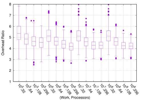
Figure 1 plots the overhead ratio according to each couple $(\mathcal{W},p)$, for a latency of $262$ (1000 runs). Similar observations have been observed with all values of latency used. The x-axis is $(\mathcal{W},p)$ for all values of $\mathcal{W}$ and $p$ intervals and the y-axis shows the overhead ratio. We use here a BoxPlot graphical method to present the results. BoxPlots give a good overview and a numerical summary of a data set. The “interquartile range” in the middle part of the plot represents the middle quartiles where 50% of the results are presented. The line inside the box presents the median. The whiskers on either side of the IQR represent the lowest and highest quartiles of the data. The ends of the whiskers represent the maximum and minimum of the data, and the individual points beyond the whiskers represent outliers.

We observe that our bound is systematically about 4 to 5.5 times greater to the one computed by simulation (depending on the range of parameters). The ratio between the two bounds decreases with the number of processors but seems fairly independent to $\mathcal{W}$.

5.3. Discussion

The challenge of this paper is to analyze WS algorithm with an explicit latency. We presented a new analysis which derives a bound on the expected Makespan for a given $\mathcal{W}$, $p$ and $\lambda$. It shows that the expected Makespan is bounded by $\mathcal{W}/p$ plus an additional term bounded by $4\gamma\approx 16$ times $\lambda\log_{2}(\mathcal{W}/(2\lambda))$. As observed in Figure 1, the constant $4\gamma$ is about four to five times larger than the one observed by simulation. A more precise fitting based on simulation results leads to the expression $\mathcal{W}/p+3.8\lambda\log_{2}(\mathcal{W}/\lambda)$. We briefly review here the main steps of the proof involving approximations and conclude with a simple fit of results on the best constant matching the expected Makespan.

First, recall that our analysis relies on $r_{k}$, the number of steal requests arriving at each time interval. The exact values of all $r_{k}$ are unknown and we rely on worst case majorations. In the proof of Theorem 4.1 we define $\gamma$ as the maximal value of $\frac{r}{-p\log_{2}(h(r))}$. The function $r\mapsto\frac{r}{-p\log_{2}(h(r))}$ is about $2.8$ for small values of $r$ and tends to $4.03$ when the number of work requests $r$ is maximal. In the simulation, we observe that the number of work requests is often low. Therefore, our definition of $\gamma$ probably contributes a factor $4/2.8\approx 1.4$ to the overhead ratio.

The second approximation done is while we computed the diminution of the potential using the maximum diminution in all cases described in the proof of Lemma 4.2. This analysis could be improved by taking a more complex potential function but this will lead to much harder computations for marginal improvements.

The third approximation is that we assumed that we do not know when exactly steal requests arrive in the interval. We therefore always took the worst case (arrivals at the end of the intervals). We believe that this approximation has only a minor effect on the overhead ratio since it mainly impacts the potential diminution obtained from computations (as opposed to stealing).

Finally, the value of $\gamma$ depends on $p$. To achieve a constant bound, we consider again the worst case obtained as $p$ tends to infinity. This explains the fact that the overhead ratio increases slightly when the number of processors decreases ($4.5$ for $256$ processors and $5$ for $32$ processors).

6. Conclusion

We presented in this paper a new analysis of Work Stealing algorithm where each communication has a communication latency of $\lambda$. Our main result was to show that the expected Makespan of a load of $W$ on a cluster of $p$ processors is bounded by $W/p+16.12\lambda\log_{2}(W/(2\lambda))$.

We based our analysis on potential functions to bound the expected number of steal requests. We therefore derived a theoretical bound on the expected Makespan. We also extend this analysis one step further, by providing a bound on the probability to exceed the bound of the Makespan.

To assess the tightness of this analysis we developed an ad-hoc simulator. We showed by comparing the theoretical bound and the experimental results that our bound is realistic. We observed moreover that our bound (established on worst case analysis) is 5 times greater than the experimental results and it is stable for all the tested values.

This work will certainly be the basis of incoming studies on more complex hierarchical topologies where communications matter. As such, it is important as it allows a full understanding of the behavior of various Work Stealing implementations in a base setting.

References

- (1)
- Agrawal et al. (2010) K. Agrawal, C. E. Leiserson, and J. Sukha. 2010. Executing task graphs using work-stealing. In 2010 IEEE International Symposium on Parallel Distributed Processing (IPDPS). 1–12. https://doi.org/10.1109/IPDPS.2010.5470403
- Arafat et al. (2016) Humayun Arafat, James Dinan, Sriram Krishnamoorthy, Pavan Balaji, and P. Sadayappan. 2016. Work Stealing for GPU-accelerated Parallel Programs in a Global Address Space Framework. Concurr. Comput. : Pract. Exper. 28, 13 (Sept. 2016), 3637–3654. https://doi.org/10.1002/cpe.3747
- Arora et al. (2001) Nimar S. Arora, Robert D. Blumofe, and C. Greg Plaxton. 2001. Thread Scheduling for Multiprogrammed Multiprocessors. In In Proceedings of the Tenth Annual ACM Symposium on Parallel Algorithms and Architectures (SPAA), Puerto Vallarta. 119–129.
- Bender and Rabin (2002) Michael A. Bender and Michael O. Rabin. 2002. Online Scheduling of Parallel Programs on Heterogeneous Systems with Applications to Cilk. Theory of Computing Systems 35, 3 (2002), 289–304. https://doi.org/10.1007/s00224-002-1055-5
- Berenbrink et al. (2003) Petra Berenbrink, Tom Friedetzky, and Leslie Ann Goldberg. 2003. The Natural Work-Stealing Algorithm is Stable. SIAM J. Comput. 32, 5 (2003), 1260–1279. https://doi.org/10.1137/S0097539701399551 arXiv:http://dx.doi.org/10.1137/S0097539701399551
- Blumofe and Leiserson (1999) Robert D. Blumofe and Charles E. Leiserson. 1999. Scheduling Multithreaded Computations by Work Stealing. J. ACM 46, 5 (Sept. 1999), 720–748. https://doi.org/10.1145/324133.324234
- Cosnard and Trystram (1995) Michel Cosnard and Denis Trystram. 1995. Parallel algorithms and architectures. International Thomson.
- Dinan et al. (2009) James Dinan, D. Brian Larkins, P. Sadayappan, Sriram Krishnamoorthy, and Jarek Nieplocha. 2009. Scalable Work Stealing. In Proceedings of the Conference on High Performance Computing Networking, Storage and Analysis (SC ’09). ACM, New York, NY, USA, Article 53, 11 pages. https://doi.org/10.1145/1654059.1654113
- Durrett (1996) Richard Durrett. 1996. Probability: theory and examples. (1996).
- Frigo et al. (1998) Matteo Frigo, Charles E. Leiserson, and Keith H. Randall. 1998. The Implementation of the Cilk-5 Multithreaded Language. SIGPLAN Not. 33, 5 (May 1998), 212–223. https://doi.org/10.1145/277652.277725
- Gast and Bruno (2010) Nicolas Gast and Gaujal Bruno. 2010. A Mean Field Model of Work Stealing in Large-scale Systems. SIGMETRICS Perform. Eval. Rev. 38, 1 (June 2010), 13–24. https://doi.org/10.1145/1811099.1811042
- Gautier et al. (2007) Thierry Gautier, Xavier Besseron, and Laurent Pigeon. 2007. KAAPI: A Thread Scheduling Runtime System for Data Flow Computations on Cluster of Multi-processors. In Proceedings of the 2007 International Workshop on Parallel Symbolic Computation (PASCO ’07). ACM, New York, NY, USA, 15–23. https://doi.org/10.1145/1278177.1278182
- Guo et al. (2010) Y. Guo, J. Zhao, V. Cave, and V. Sarkar. 2010. SLAW: A scalable locality-aware adaptive work-stealing scheduler. In 2010 IEEE International Symposium on Parallel Distributed Processing (IPDPS). 1–12. https://doi.org/10.1109/IPDPS.2010.5470425
- Hamid et al. (2015a) N. Hamid, R. Walters, and G. Wills. 2015a. Simulation and Mathematical Analysis of Multi-core Cluster Architecture. In 2015 17th UKSim-AMSS International Conference on Modelling and Simulation (UKSim). 476–481. https://doi.org/10.1109/UKSim.2015.54
- Hamid et al. (2015b) Norhazlina Hamid, Robert John Walters, and Gary Brian Wills. 2015b. An analytical model of multi-core multi-cluster architecture (MCMCA). (2015), 12 pages. http://eprints.soton.ac.uk/374744/
- jai Min et al. (2011) Seung jai Min, Costin Iancu, and Katherine Yelick. 2011. Hierarchical Work Stealing on Manycore Clusters. In In: Fifth Conference on Partitioned Global Address Space Programming Models. Galveston Island.
- Leiserson (2009) Charles E. Leiserson. 2009. The Cilk++ Concurrency Platform. In Proceedings of the 46th Annual Design Automation Conference (DAC ’09). ACM, New York, NY, USA, 522–527. https://doi.org/10.1145/1629911.1630048
- Li et al. (2013) S. Li, J. Hu, X. Cheng, and C. Zhao. 2013. Asynchronous Work Stealing on Distributed Memory Systems. In 2013 21st Euromicro International Conference on Parallel, Distributed, and Network-Based Processing. 198–202. https://doi.org/10.1109/PDP.2013.35
- Lüling and Monien (1993) Reinhard Lüling and Burkhard Monien. 1993. A Dynamic Distributed Load Balancing Algorithm with Provable Good Performance. In Proceedings of the Fifth Annual ACM Symposium on Parallel Algorithms and Architectures (SPAA ’93). ACM, New York, NY, USA, 164–172. https://doi.org/10.1145/165231.165252
- Mitzenmacher (1998) Michael Mitzenmacher. 1998. Analyses of Load Stealing Models Based on Differential Equations. In Proceedings of the Tenth Annual ACM Symposium on Parallel Algorithms and Architectures (SPAA ’98). ACM, New York, NY, USA, 212–221. https://doi.org/10.1145/277651.277687
- Muller and Acar (2016) Stefan K. Muller and Umut A. Acar. 2016. Latency-Hiding Work Stealing: Scheduling Interacting Parallel Computations with Work Stealing. In Proceedings of the 28th ACM Symposium on Parallelism in Algorithms and Architectures (SPAA ’16). ACM, New York, NY, USA, 71–82. https://doi.org/10.1145/2935764.2935793
- Perarnau and Sato (2014) S. Perarnau and M. Sato. 2014. Victim Selection and Distributed Work Stealing Performance: A Case Study. In 2014 IEEE 28th International Parallel and Distributed Processing Symposium. 659–668. https://doi.org/10.1109/IPDPS.2014.74
- Robison et al. (2008) A. Robison, M. Voss, and A. Kukanov. 2008. Optimization via Reflection on Work Stealing in TBB. In 2008 IEEE International Symposium on Parallel and Distributed Processing. 1–8. https://doi.org/10.1109/IPDPS.2008.4536188
- Rudolph et al. (1991) Larry Rudolph, Miriam Slivkin-Allalouf, and Eli Upfal. 1991. A Simple Load Balancing Scheme for Task Allocation in Parallel Machines. In Proceedings of the Third Annual ACM Symposium on Parallel Algorithms and Architectures (SPAA ’91). ACM, New York, NY, USA, 237–245. https://doi.org/10.1145/113379.113401
- Sanders (1999) Peter Sanders. 1999. Asynchronous Random Polling Dynamic Load Balancing. Springer Berlin Heidelberg, Berlin, Heidelberg, 37–48. https://doi.org/10.1007/3-540-46632-0_5
- Tchiboukdjian et al. (2013) Marc Tchiboukdjian, Nicolas Gast, and Denis Trystram. 2013. Decentralized list scheduling. Annals of Operations Research 207, 1 (2013), 237–259. https://doi.org/10.1007/s10479-012-1149-7
- Yang and He (2017) Jixiang Yang and Qingbi He. 2017. Scheduling Parallel Computations by Work Stealing: A Survey. International Journal of Parallel Programming (2017), 1–25. https://doi.org/10.1007/s10766-016-0484-8