Off-spectral analysis of Bergman kernels

Abstract.

The asymptotic analysis of Bergman kernels with respect to exponentially varying measures near emergent interfaces has attracted recent attention. Such interfaces typically occur when the associated limiting Bergman density function vanishes on a portion of the plane, the off-spectral region. This type of behavior is observed when the metric is negatively curved somewhere, or when we study partial Bergman kernels in the context of positively curved metrics. In this work, we cover these two situations in a unified way, for exponentially varying weights on the complex plane. We obtain a uniform asymptotic expansion of the coherent state of depth $n$ rooted at an off-spectral point, which we also refer to as the root function at the point in question. The expansion is valid in the entire off-spectral component containing the root point, and protrudes into the spectrum as well. This allows us to obtain error function transition behavior of the density of states along the smooth interface. Previous work on asymptotic expansions of Bergman kernels is typically local, and valid only in the bulk region of the spectrum, which contrasts with our non-local expansions.

1. Introduction

1.1. Bergman kernels and emergent interfaces

This article is a companion to our recent work [13] on the structure of planar orthogonal polynomials. We will make frequent use of methods developed there, and recommend that the reader keep that article available for ease of reference.

The study of Bergman kernel asymptotics has by now a sizeable literature. The majority of the contributions have the flavor of local asymptotics near a given point $w_{0}$, under a positive curvature condition. However, in the study of partial Bergman kernels for the subspace of all functions vanishing to a given order at the point $w_{0}$, the assumption of vanishing has the effect of introducing a negative point mass for the curvature form at $w_{0}$. In addition to the negative curvature which comes from considering partial Bergman kernels defined by vanishing, we allow for the direct effect of patches of negatively curved geometry. Around the set of negative curvature, a forbidden region (or off-spectral set) emerges. This forbidden region is typically larger than the set of actual negative curvature, and may consist of several connectivity components. Recently, the asymptotic behavior of Bergman kernels near the interface at the edge of the forbidden region has attracted considerable attention. In this work, we intend to investigate this in the fairly general setting of exponentially varying weights in the complex plane. The restriction of the Bergman kernel to the diagonal gives us the density of states, which drops steeply at the interface. Indeed, in the forbidden region the density of states vanishes asymptotically, with exponential decay. One of our main results is that the density of states across the interface converges to the error function in a blow-up, provided the interface is smooth.

The key to obtaining the above-mentioned result is in fact our main result. It concerns the expansion of the coherent state $\mathrm{k}_{n}(z,w_{0})$ of depth $n$ at a given off-spectral point $w_{0}$. This is the renormalized reproducing kernel function at the point $w_{0}$ for the Bergman space defined by vanishing to order $n$ at $w_{0}$. When $n=0$, the coherent state of depth $0$ is just the normalized Bergman kernel $K(w_{0},w_{0})^{-\frac{1}{2}}K(z,w_{0})$. An important feature of the asymptotic expansion is that $z$ and $w_{0}$ are allowed to be macroscopically separated. Such truly off-diagonal expansions have, to the best of our knowledge, not appeared elsewhere. It is easy to see that the coherent state of order $n=0,1,2,\ldots$, at $w_{0}$ form an orthonormal basis for the Bergman space, which gives an expansion of the density of states, which leads to the error function asymptotics. Similarly, if we want to handle partial Bergman kernels given by vanishing to order $n_{0}$ at $w_{0}$, we expand in the basis given by the coherent states of depth $n=n_{0},n_{0}+1,\ldots$.

1.2. Coherent states and elementary potential theory

We now introduce the objects of study. The Bergman space $A^{2}_{mQ}$ is defined as the collection of all entire functions $f$ in with finite weighted $L^{2}$-norm

$$\|f\|_{mQ}^{2}:=\int_{{\mathbb{C}}}\lvert f(z)\rvert^{2}\mathrm{e}^{-2mQ(z)}\mathrm{dA}(z)<+\infty,$$

where $\mathrm{dA}$ denotes the planar area element normalized so that the unit disk ${\mathbb{D}}$ has unit area, and where $Q$ is a potential with certain growth and regularity properties (see Definition 1.6.1). We denote the reproducing kernel for $A^{2}_{mQ}$ by $K_{m}$, and for a given point $w_{0}\in{\mathbb{C}}$, we consider the coherent state (normalized Bergman kernel)

(1.2.1) $$\mathrm{k}_{m,w_{0}}(z):=K_{m}(w_{0},w_{0})^{-\frac{1}{2}}K_{m}(z,w_{0}),$$

which has norm $1$ in $A^{2}_{mQ}$. There is a notion of the spectrum $\mathcal{S}$, also called the spectral droplet. This is the closed set defined in terms of the following obstacle problem. Let $\mathrm{SH}({\mathbb{C}})$ denote the cone of all subharmonic functions on the plane ${\mathbb{C}}$, and consider the function

$$\hat{Q}(z):=\sup\big{\{}q(z)\,:\,\,q\in\mathrm{SH}({\mathbb{C}}),\,\,\text{and}\,\,\,q\leq Q\,\,\,\text{on}\,\,\,{\mathbb{C}}\big{\}}.$$

Whenever $Q$ is $C^{1,1}$-smooth and has some modest growth at infinity, it is known that $\hat{Q}\in C^{1,1}$ as well, and it is a matter of definition that $\hat{Q}\leq Q$ pointwise (see, e.g., [10]). Here, $C^{1,1}$ denotes the standard smoothness class of differentiable functions with Lipschitz continuous first order partial derivatives. We define the spectrum (or the spectral droplet) as the contact set

(1.2.2) $$\mathcal{S}:=\big{\{}z\in{\mathbb{C}}\,:\,\hat{Q}(z)=Q(z)\big{\}}.$$

The forbidden region is the complement $\mathcal{S}^{c}={\mathbb{C}}\setminus\mathcal{S}$.

We will need these notions in the context of partial Bergman kernels as well. For a non-negative integer $n$ and a point $w_{0}\in{\mathbb{C}}$, we consider the subspace $A^{2}_{mQ,n,w_{0}}$ of $A^{2}_{mQ}$, consisting of those functions that vanish to order at least $n$ at $w_{0}$. It may happen for some $n$ that this space is trivial, for instance when the potential $Q$ has logarithmic growth only, because then the space $A^{2}_{mQ}$ consists of polynomials of a bounded degree. We denote its reproducing kernel by $K_{m,n,w_{0}}$, and observe that $K_{m,0,w_{0}}=K_{m}$. We shall need also the coherent state of depth $n$ at $w_{0}$ (or the root function of order $n$), denoted $\mathrm{k}_{m,n,w_{0}}$, which is the unique solution to the optimization problem

$$\max\big{\{}\operatorname{Re}f^{(n)}(w_{0}):\,\,f\in A^{2}_{mQ,n,w_{0}},\,\,\|f\|_{mQ}\leq 1\big{\}},$$

provided the maximum is positive, in which case the optimizer has norm $\|f\|_{mQ}=1$. In the remaining case, the maximum equals $0$, and either only $f=0$ is possible, or there are several competing optimizers, simply because we may multiply the function by unimodular constants and obtain alternative optimizers. In both remaining instances we declare that $\mathrm{k}_{m,n,w_{0}}=0$. When nontrivial, the root function (or coherent state) of order $n$ at $w_{0}$ is connected with the reproducing kernel $K_{m,n,w_{0}}$:

(1.2.3) $$\mathrm{k}_{m,n,w_{0}}(z)=\lim_{\zeta\to w_{0}}K_{m,n,w_{0}}(\zeta,\zeta)^{-1/2}K_{m,n,w_{0}}(z,\zeta),$$

where the point $\zeta$ should approach $w_{0}$ not arbitrarily but in a fashion such that the limit exists and has positive $n$-th derivative at $w_{0}$. The root function $\mathrm{k}_{m,n,w_{0}}$ will play a key role in our analysis, similar to that of the orthogonal polynomials in the context of polynomial Bergman kernels. The root functions $\mathrm{k}_{m,n,w_{0}}$ all have norm equal to $1$ in $A^{2}_{mQ}$, except when they are trivial and have norm $0$. As a result of the relation (1.2.3), we may alternatively call the root function $\mathrm{k}_{m,n,w_{0}}$ a normalized partial Bergman kernel. The spectral droplet associated to a family of partial Bergman kernels of the above type is defined in Subsection 2.1 in terms of an obstacle problem, and we briefly outline how this is done. For $0\leq\tau<+\infty$, let $\mathrm{SH}_{\tau,w_{0}}({\mathbb{C}})$ denote the convex set

$$\mathrm{SH}_{\tau,w_{0}}({\mathbb{C}})=\big{\{}q\in\mathrm{SH}\,({\mathbb{C}})\,:\,q(z)\leq\tau\log\lvert z-w_{0}\rvert+\mathrm{O}(1)\,\;\text{as }\,z\to w_{0}\big{\}},$$

so that for $\tau=0$ we recover $\mathrm{SH}({\mathbb{C}})$. We consider the corresponding obstacle problem

(1.2.4) $$\hat{Q}_{\tau,w_{0}}(z)=\sup\big{\{}q(z)\;:\;q\in\mathrm{SH}_{\tau,w_{0}}({\mathbb{C}}),\,q\leq Q\,\,\text{on}\,\,{\mathbb{C}}\big{\}},$$

and observe that $\tau\mapsto\hat{Q}_{\tau,w_{0}}$ is monotonically decreasing pointwise. We define a family of spectral droplets as the coincidence sets

(1.2.5) $$\mathcal{S}_{\tau,w_{0}}=\big{\{}z\in{\mathbb{C}}\,:\,Q(z)=\hat{Q}_{\tau,w_{0}}(z)\big{\}}.$$

Due to the monotonicity, the droplets $\mathcal{S}_{\tau,w_{0}}$ get smaller as $\tau$ increases, starting from $\mathcal{S}_{0,w_{0}}=\mathcal{S}$ for $\tau=0$. The partial Bergman density

$$\rho_{m,n,w_{0}}(z):=m^{-1}K_{m,n,w_{0}}(z,z)\,\mathrm{e}^{-2mQ(z)},\qquad z\in{\mathbb{C}},$$

may be viewed as the normalized local dimension of the space $A^{2}_{mQ,n,w_{0}}({\mathbb{C}})$, and, in addition, it has the interpretation as the intensity of a corresponding (possibly infinite) Coulomb gas. In the case $n=0$ we omit the word “partial” and speak of the Bergman density. It is known that in the limit as $m,n\to+\infty$ with $n=m\tau$,

$$\rho_{m,n,w_{0}}(z)\to 2\varDelta Q(z)\,1_{\mathcal{S}_{\tau,w_{0}}}(z),$$

in the sense of convergence of distributions. In particular, $\varDelta Q\geq 0$ holds a.e. on $\mathcal{S}$. Here, we write $\varDelta$ for differential operator $\partial\bar{\partial}$, which is one quarter of the usual Laplacian. The above convergence reinforces our understanding of the droplets $\mathcal{S}_{\tau,w_{0}}$ as spectra, in the sense that the Coulomb gas may be thought to model eigenvalues (at least in the finite-dimensional case). The bulk of the spectral droplet $\mathcal{S}_{\tau,w_{0}}$ is the set

$$\{z\in\mathrm{int}(\mathcal{S}_{\tau,w_{0}}):\,\varDelta Q(z)>0\},$$

where “int” stands for the operation of taking the interior.

1.3. Further background on Bergman kernel expansions

Our motivation for the above setup originates with the theory of random matrices, specifically the random normal matrix ensembles. We should mention that an analogous situation occurs in the study of complex manifolds. The Bergman kernel then appears in the study of spaces of $L^{2}$-integrable global holomorphic sections of $L^{m}$, where $L^{m}$ is a high tensor power of a holomorphic line bundle $L$ over the manifold, endowed with an hermitian fiber metric $h$. If $\{U_{i}\}_{i}$ is a coordinate system on a manifold, then a holomorphic section $s$ to a line bundle $L$ can be written in local coordinates as $s=s_{i}e_{i}$, where $e_{i}$ are local basis elements for $L$ and $s_{i}$ are holomorphic functions. The pointwise norm of a section $s$ of $L^{m}$ may be then be written as $\lvert s\rvert_{h^{m}}^{2}=\lvert s_{i}\rvert^{2}\mathrm{e}^{-m\phi_{i}}$ on $U_{i}$, for some smooth real-valued functions $\phi_{i}$. Along with a volume form on the base manifold, this defines an $L^{2}$ space which shares many characteristics with the spaces considered here.

The asymptotic behavior of Bergman kernels has been the subject of intense investigation. However, the understanding has largely been limited to the analysis of the kernel inside the bulk of the spectrum, in which case the kernel enjoys a full local asymptotic expansion. The pioneering work on Bergman kernel asymptotics begins with the efforts by Hörmander [14] and Fefferman [8]. Developing further the microlocal approach of Hörmander, Boutet de Monvel and Sjöstrand [5] obtain a near-diagonal expansion of the Bergman kernel close to the boundary of the given domain. Later, in the context of Kähler geometry, the influential peak section method was introduced by Tian [20]. His results were refined further by Catlin and Zelditch [6, 21], while the connection with microlocal analysis was greatly simplified in the more recent work by Berman, Berndtsson, and Sjöstrand [4]. A key element of all these methods is that the kernel is determined by the local geometry around the given point. This property is absent when we consider the kernel near an off-spectral point or near a boundary point of the spectral droplet.

In the recent work [13], we analyze the boundary behavior of polynomial Bergman kernels, for which the corresponding spectral droplet is compact, connected, and has a smooth Jordan curve as boundary. The analysis takes the path via a full asymptotic expansion of the orthogonal polynomials, valid off a sequence of increasing compacts which eventually fill the droplet. By expanding the polynomial kernel in the orthonormal basis provided by the orthogonal polynomials, the error function asymptotics emerges along smooth spectral boundaries.

The appearance of an interface for partial Bergman kernels in higher dimensional settings and in the context of complex manifolds has been observed more than once, notably in the work by Shiffman and Zelditch [19] and by Pokorny and Singer [15]. That the error function governs the transition behavior across the interface was observed later in several contexts. For instance, in [16], Ross and Singer investigate the partial Bergman kernels associated to spaces of holomorphic sections vanishing along a divisor, and obtain error function transition behavior under the assumption that the set-up is invariant under a holomorphic $S^{1}$-action. This result was later extended by Zelditch and Zhou [22], in the context of $S^{1}$-symmetry. More recently, Zelditch and Zhou [23] obtain the same transition for so-called spectral partial Bergman kernels, defined in terms of the Toeplitz quantization of a general smooth Hamiltonian.

Our methods for obtaining asymptotic expansions of coherent states centered at off-spectral points do not easily extend to the higher complex dimensional setting. It appears plausible, however, that our analysis would apply when the complex plane ${\mathbb{C}}$ is replaced by a compact Riemann surface with one or possibly several punctures.

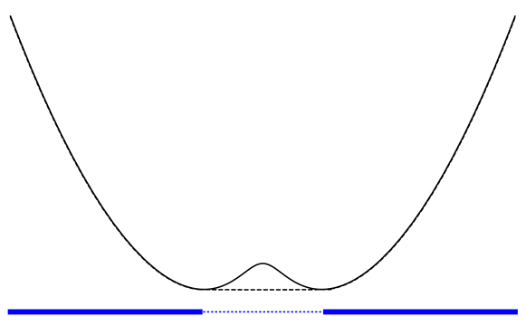
Figure 1.1. Illustration of the spectral droplet corresponding to the potential $Q(z)=\lvert z\rvert^{2}-\log(a+\lvert z\rvert^{2})$, with $a=0.04$. The spectrum is illustrated with a thick line, and appears as the contact set between $Q$ (solid) and the solution $\hat{Q}$ to the obstacle function (dashed).

1.4. Off-spectral and off-diagonal asymptotics of coherent states

The main contribution of the present work, put in the planar context, is a non-local asymptotic expansion of coherent states centered at an off-spectral point. For ease of exposition, we begin with a version that requires as few prerequisites as possible for the formulation. We denote by $Q(z)$ an admissible potential, by which we mean the following:

1. $Q:{\mathbb{C}}\to{\mathbb{R}}$ is $C^{2}$-smooth, and has sufficient growth at infinity:

   $$\tau_{Q}:=\liminf_{\lvert z\rvert\to+\infty}\frac{Q(z)}{\log\lvert z\rvert}>0.$$

2. $Q$ is real-analytically smooth and strictly subharmonic in a neighborhood of $\partial\mathcal{S}$, where $\mathcal{S}$ is the contact set of (1.2.2),

3. there exists a bounded component $\Omega$ of the complement $\mathcal{S}^{c}={\mathbb{C}}\setminus\mathcal{S}$ which is simply connected, and has real-analytically smooth Jordan curve boundary.

We consider the case when there exists a non-trivial off-spectral component $\Omega$ which is bounded and simply connected, with real-analytic boundary, and pick a “root point” $w_{0}\in\Omega$. To be precise, by an off-spectral component we mean a connectivity component of the complement $\mathcal{S}^{c}$. This situation occurs, e.g., if the potential is strictly superharmonic in a portion of the plane, as is illustrated in Figure 1.1. In terms of the metric, this means that there is a region where the curvature is negative.

A word on notation. To formulate our first main result, we need the function ${\mathcal{Q}}_{w_{0}}$, which is bounded and holomorphic in the off-spectral component $\Omega$ and whose real part equals $Q$ along the boundary $\partial\Omega$. To fix the imaginary part, we require that ${\mathcal{Q}}_{w_{0}}(w_{0})\in{\mathbb{R}}$. In addition, we need the conformal mapping $\varphi_{w_{0}}$ which takes $\Omega$ onto the unit disk ${\mathbb{D}}$ with $\varphi_{w_{0}}(w_{0})=0$ and $\varphi_{w_{0}}^{\prime}(w_{0})>0$. Since the boundary $\partial\Omega$ is assumed to be a real-analytically smooth Jordan curve, both the function ${\mathcal{Q}}_{w_{0}}$ and the conformal mapping $\varphi_{w_{0}}$ extend analytically across $\partial\Omega$ to a fixed larger domain. By possibly considering a smaller fixed larger domain, we may assume that the extended function $\varphi_{w_{0}}$ is conformal on the larger region. These observations are essential for our first main result, since we want the asymptotics to hold across the interface $\partial\Omega$.

Theorem 1.4.1.

Assuming that $Q$ is an admissible potential, we have the following. Given a positive integer $\kappa$ and a positive real $A$, there exist a neighborhood $\Omega^{\circledast}$ of the closure of $\Omega$ and bounded holomorphic functions ${\mathcal{B}}_{j,w_{0}}$ on $\Omega^{\circledast}$ for $j=0,\ldots,\kappa$, as well as domains $\Omega_{m}=\Omega_{m,A}$ with $\Omega\subset\Omega_{m}\subset\Omega^{\circledast}$ which meet

$$\mathrm{dist}_{{\mathbb{C}}}(\partial\Omega_{m},\partial\Omega)\geq A\,m^{-\frac{1}{2}}(\log m)^{\frac{1}{2}},$$

such that the normalized Bergman kernel at the point $w_{0}$ enjoys the asymptotic expansion

$$\mathrm{k}_{m}(z,w_{0})=\frac{K_{m}(z,w_{0})}{K_{m}(w_{0},w_{0})^{1/2}}\\ =m^{\frac{1}{4}}(\varphi_{w_{0}}^{\prime}(z))^{\frac{1}{2}}\mathrm{e}^{m{\mathcal{Q}}_{w_{0}}(z)}\bigg{\{}\sum_{j=0}^{\kappa}m^{-j}{\mathcal{B}}_{j,w_{0}}(z)+\mathrm{O}\big{(}m^{-\kappa-1}\big{)}\bigg{\}},$$

as $m\to+\infty$, where the error term is uniform on $\Omega_{m}$. Here, the main term ${\mathcal{B}}_{0,w_{0}}$ is obtained as the unique zero-free holomorphic function on $\Omega$ which is smooth up to the boundary with ${\mathcal{B}}_{0,w_{0}}(w_{0})>0$, and with prescribed boundary modulus

$$\lvert{\mathcal{B}}_{0,w_{0}}(z)\rvert=\pi^{-\frac{1}{4}}[\varDelta Q(z)]^{\frac{1}{4}},\qquad z\in\partial\Omega.$$

Moreover, if $A$ is big enough, then

$$\int_{\Omega_{m}}|\mathrm{k}_{m,w_{0}}(z)|^{2}\mathrm{e}^{-2mQ(z)}\mathrm{dA}(z)=1+\mathrm{O}(m^{-\kappa}).$$

As an illustration of this result, we show the Gaussian wave character of the Berezin density $\mathrm{k}_{m}(w_{0},w_{0})^{-1}|\mathrm{k}_{m}(z,w_{0})|^{2}\mathrm{e}^{-2mQ(z)}$ in Figure 1.2.

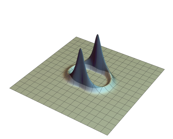
Figure 1.2. Illustration of the the Gaussian wave asymptotics of the probability density associated to the coherent state $\mathrm{k}_{m,0,0}(z)$, where $Q(z)=\frac{1}{2}|z|^{-2}-\frac{1}{8}\operatorname{Re}(z^{-2})+\log|z|$. The root point is at the origin, and the asymptotics of Theorem 1.4.1 are valid in the domain $\Omega$ (inside the ridge) including a neighborhood of the boundary $\partial\Omega$ of width proportional to $(m^{-1}\log m)^{\frac{1}{2}}$.

Remark 1.4.2.

Using an approach based on Laplace’s method, the functions ${\mathcal{B}}_{j,w_{0}}$ may be obtained algorithmically, for $j=1,2,3,\ldots$, see Theorem 3.2.2 below. The details of the algorithm are analogous with the case of the orthogonal polynomials presented in [13].

Commentary to the theorem. The point $w_{0}$ may be chosen as any fixed point in $\Omega$, while the point $z$ is allowed to vary anywhere inside the set $\Omega_{m}$, which contains the entire off-spectral component $\Omega$ as well as a shrinking neighborhood of the boundary $\partial\Omega$. Hence, we obtain macroscopically off-diagonal asymptotics, where the points $z$ and $w_{0}$ are either both off-spectral, or where $z$ is spectral near-boundary and $w_{0}$ off-spectral, respectively. To our knowledge, this is the first instance of such asymptotics. Indeed, earlier work covers either diagonal or near-diagonal asymptotics inside the bulk of the spectrum. The analysis of Bergman kernel asymptotics for two macroscopically separated points in the bulk $\mathcal{S}^{\circ}$ appears difficult if we ask for high precision, and the same can be said for the case when $w_{0}\in\Omega$ is off-spectral and $z\in\mathcal{S}^{\circ}$ is a bulk point. To address the latter issue, we may ask what happens in Theorem 1.4.1 if $z$ is not in the set $\Omega_{m}$. Since $\Omega_{m}$ captures most of the $L^{2}$-mass of the root function in view of Theorem 1.4.1, we see that the coherent state is minuscule outside $\Omega_{m}$ in the $L^{2}$-sense. If we want corresponding pointwise control, we may appeal to e.g. the subharmonicity estimate of Lemma  3.2 of [1].

1.5. Expansion of partial Bergman kernels in terms of root functions

For a $(\tau,w_{0})$-admissible potential, the partial Bergman kernel $K_{m,n,w_{0}}$ with the root point $w_{0}$ is well-defined and nontrivial. In analogy with Taylor’s formula, it enjoys an expansion in terms of the root functions $\mathrm{k}_{m,n^{\prime},w_{0}}$ for $n^{\prime}\geq n$.

Theorem 1.5.1.

Under the above assumption of $(\tau,w_{0})$-admissibility of $Q$, we have that

$$K_{m,n,w_{0}}(z,w)=\sum_{n^{\prime}=n}^{+\infty}\mathrm{k}_{m,n^{\prime},w_{0}}(z)\overline{\mathrm{k}_{m,n^{\prime},w_{0}}(w)},\qquad(z,w)\in{\mathbb{C}}\times{\mathbb{C}}.$$

Proof.

For $n^{\prime},n^{\prime\prime}\geq n$ with $n^{\prime\prime}<n^{\prime}$, the functions $\mathrm{k}_{m,n^{\prime},w_{0}}$ and $\mathrm{k}_{m,n^{\prime\prime},w_{0}}$ are orthogonal in $A^{2}_{mQ}$. If one of them is trivial, orthogonality is immediate, while if both are nontrivial, we argue as follows. Let $\zeta^{\prime},\zeta^{\prime\prime}\in{\mathbb{C}}$ be close to $w_{0}$, and calculate that

$$K_{m,n^{\prime},w_{0}}(\zeta^{\prime},\zeta^{\prime})^{-\frac{1}{2}}K_{m,n^{\prime\prime},w_{0}}(\zeta^{\prime\prime},\zeta^{\prime\prime})^{-\frac{1}{2}}\big{\langle}K_{m,n^{\prime},w_{0}}(\cdot,\zeta^{\prime}),K_{m,n^{\prime\prime},w_{0}}(\cdot,\zeta^{\prime\prime})\big{\rangle}_{mQ}\\ =K_{m,n^{\prime},w_{0}}(\zeta^{\prime},\zeta^{\prime})^{-\frac{1}{2}}K_{m,n^{\prime\prime},w_{0}}(\zeta^{\prime\prime},\zeta^{\prime\prime})^{-\frac{1}{2}}K_{m,n^{\prime},w_{0}}(\zeta^{\prime\prime},\zeta^{\prime})=\mathrm{O}(|\zeta^{\prime\prime}-w_{0}|^{n^{\prime}-n^{\prime\prime}}),$$

which tends to $0$ as $\zeta^{\prime\prime}\to w_{0}$. The claimed orthogonality follows. Moreover, since the root functions $\mathrm{k}_{m,n^{\prime},w_{0}}$ have unit norm when nontrivial, the expression

$$\sum_{n^{\prime}=n}^{+\infty}\mathrm{k}_{m,n^{\prime},w_{0}}(z)\overline{\mathrm{k}_{m,n^{\prime},w_{0}}(w)}$$

equals the reproducing kernel function for the Hilbert space with the norm of $A^{2}_{mQ}$ spanned by the vectors $\mathrm{k}_{m,n^{\prime},w_{0}}$ with $n^{\prime}\geq n$. It remains to check that this is the whole partial Bergman space $A^{2}_{mQ,n,w_{0}}$. To this end, let $f\in A^{2}_{mQ,n,w_{0}}$ be orthogonal to all the the vectors $\mathrm{k}_{m,n^{\prime},w_{0}}$ with $n^{\prime}\geq n$. By the definition of the space $A^{2}_{mQ,n,w_{0}}$, this means that $f(z)=\mathrm{O}(|z-w_{0}|^{n})$ near $w_{0}$. If $f$ is nontrivial, there exists an integer $N\geq n$ such that $f(z)=c\,(z-w_{0})^{N}+\mathrm{O}(|z-w_{0}|^{N+1})$ near $w_{0}$, where $c\neq 0$ is complex. At the same time, the existence of such nontrivial $f$ entails that the corresponding root functions $\mathrm{k}_{m,N,w_{0}}$ is nontrivial as well, and that $K_{m,N,w_{0}}(\zeta,\zeta)\asymp|\zeta-w_{0}|^{2N}$ for $\zeta$ near $w_{0}$. On the other hand, the orthogonality between $f$ and $\mathrm{k}_{m,N,w_{0}}$ gives us that

$$0=\langle f,\mathrm{k}_{m,N,w_{0}}\rangle_{mQ}=\lim_{\zeta\to w_{0}}K_{m,N,w_{0}}(\zeta,\zeta)^{-\frac{1}{2}}\big{\langle}f,K_{m,N,w_{0}}(\cdot,\zeta)\big{\rangle}_{mQ}\\ =\lim_{\zeta\to w_{0}}K_{m,N,w_{0}}(\zeta,\zeta)^{-\frac{1}{2}}f(\zeta)$$

where we approach $w_{0}$ only in an appropriate direction so that the limit exists. But this contradicts the given asymptotic behavior of $f(\zeta)$ near $w_{0}$, since $c\neq 0$ tells us that any limit of the right-hand side would be nonzero. ∎

1.6. Off-spectral asymptotics of partial Bergman kernels

Given a point $w_{0}\in{\mathbb{C}}$ we recall the partial Bergman spaces $A^{2}_{mQ,n,w_{0}}$, and the associated spectral droplets $\mathcal{S}_{\tau,w_{0}}$ (see (1.2.5)), where we keep $n=\tau m$. Before we proceed with the formulation of the second result, let us fix some terminology.

Definition 1.6.1.

A real-valued potential $Q$ is said to be $(\tau,w_{0})$-admissible if the following conditions hold:

1. $Q:{\mathbb{C}}\to{\mathbb{R}}$ is $C^{2}$-smooth and has sufficient growth at infinity:

   $$\tau_{Q}:=\liminf_{\lvert z\rvert\to+\infty}\frac{Q(z)}{\log\lvert z\rvert}>0.$$

2. $Q$ is real-analytically smooth and strictly subharmonic in a neighborhood of $\partial\mathcal{S}_{\tau,w_{0}}$.

3. The point $w_{0}$ is an off-spectral point, i.e., $w_{0}\notin\mathcal{S}_{\tau,w_{0}}$, and the component $\Omega_{\tau,w_{0}}$ of the complement $\mathcal{S}_{\tau,w_{0}}^{c}$ containing the point $w_{0}$ is bounded and simply connected, with real-analytically smooth Jordan curve boundary.

If for an interval $I\subset[0,+\infty[$, the potential $Q$ is $(\tau,w_{0})$-admissible for each $\tau\in I$ and $\{\Omega_{\tau,w_{0}}\}_{\tau\in I}$ is a smooth flow of domains, then $Q$ is said to be $(I,w_{0})$-admissible.

Generally speaking, off-spectral components may be unbounded. It is for reasons of simplicity that we focus on bounded off-spectral components in the above definition.

A word on notation. We will assume in the sequel that $Q$ is $(I,w_{0})$-admissible for some non-trivial compact interval $I=I_{0}$. For an illustration of the situation, see Figure 1.3.

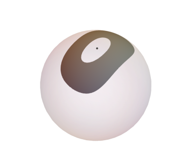
Figure 1.3. Illustration of a spectral droplet (shaded) in the Riemann sphere with two off-spectral components of the complement. The point $w_{0}$ is indicated by the dot near the north pole, and the connectivity component of the off-spectral set containing $w_{0}$ is denoted by $\Omega_{w_{0}}$.

We let $\varphi_{\tau,w_{0}}$ denote the surjective Riemann mapping

(1.6.1) $$\varphi_{\tau,w_{0}}\colon\Omega_{\tau,w_{0}}\to{\mathbb{D}},\quad\varphi_{\tau,w_{0}}(0)=0,\quad\varphi_{\tau,w_{0}}^{\prime}(0)>0,$$

which by our smoothness assumption on the boundary $\partial\Omega_{\tau,w_{0}}$ extends conformally across $\partial\Omega_{\tau,w_{0}}$. We denote by $\mathcal{Q}_{\tau,w_{0}}$ the bounded holomorphic function in $\Omega_{\tau,w_{0}}$ whose real part equals $Q$ on $\partial\Omega_{\tau,w_{0}}$ and is real-valued at $w_{0}$. It is tacitly assumed to extend holomorphically across the boundary $\partial\Omega_{\tau,w_{0}}$. We now turn to our second main result.

Theorem 1.6.2.

Assume that the potential $Q$ is $(I_{0},w_{0})$-admissible, where the interval $I_{0}$ is compact. Given a positive integer $\kappa$ and a positive real $A$, there exists a neighborhood $\Omega^{\circledast}_{\tau,w_{0}}$ of the closure of $\Omega_{\tau,w_{0}}$ and bounded holomorphic functions ${\mathcal{B}}_{j,\tau,w_{0}}$ on $\Omega^{\circledast}_{\tau,w_{0}}$, as well as domains $\Omega_{\tau,w_{0},m}=\Omega_{\tau,w_{0},m,A}$ with $\Omega_{\tau,w_{0}}\subset\Omega_{\tau,w_{0},m}\subset\Omega^{\circledast}_{\tau,w_{0}}$ which meet

$$\mathrm{dist}_{{\mathbb{C}}}(\Omega_{\tau,w_{0},m}^{c},\Omega_{\tau,w_{0}})\geq Am^{-\frac{1}{2}}(\log m)^{\frac{1}{2}},$$

such that the root function of order $n$ at $w_{0}$ enjoys the expansion

$$\mathrm{k}_{m,n,w_{0}}(z)=m^{\frac{1}{4}}(\varphi_{\tau,w_{0}}^{\prime}(z))^{\frac{1}{2}}(\varphi_{\tau,w_{0}}(z))^{n}\mathrm{e}^{m{\mathcal{Q}}_{\tau,w_{0}}(z)}\bigg{\{}\sum_{j=0}^{\kappa}m^{-j}{\mathcal{B}}_{j,\tau,w_{0}}(z)+\mathrm{O}(m^{-\kappa-1})\bigg{\}}$$

on $\Omega_{\tau,w_{0},m}$ as $n=\tau m\to+\infty$ while $\tau\in I_{0}$, where the error term is uniform. Here, the main term ${\mathcal{B}}_{0,\tau,w_{0}}$ is zero-free and smooth up to the boundary on $\Omega_{\tau,w_{0}}$ with ${\mathcal{B}}_{0,\tau,w_{0}}(w_{0})>0$, and with prescribed boundary modulus

$$\lvert{\mathcal{B}}_{0,\tau,w_{0}}(\zeta)\rvert=\pi^{-\frac{1}{4}}[\varDelta Q(\zeta)]^{\frac{1}{4}},\qquad\zeta\in\partial\Omega_{\tau,w_{0}}.$$

Moreover, for $A$ big enough, we have

$$\int_{\Omega_{\tau,w_{0},m}}|\mathrm{k}_{m,n,w_{0}}(z)|^{2}\mathrm{e}^{-2mQ(z)}\mathrm{dA}(z)=1+\mathrm{O}(m^{-\kappa})$$

as $n=\tau m\to+\infty$.

Remark 1.6.3.

As in the case of the normalized Bergman kernels, the expressions ${\mathcal{B}}_{j,\tau,w_{0}}$ may be obtained algorithmically, for $j=1,2,3,\ldots$ (see Theorem 3.2.2 below).

Commentary to the theorem. (a) As in Theorem 1.4.1, the point $w_{0}$ may be chosen as any fixed point in $\Omega$, while the point $z$ is allowed to vary anywhere inside the set $\Omega_{\tau,w_{0},m}$. Arguing in a fashion analogous to what we did in the commentary following Theorem 1.4.1, we may conclude that $\mathrm{k}_{m,n,w_{0}}$ is small, both pointwise and in the $L^{2}$-sense, away from the set $\Omega_{\tau,w_{0},m}$.

(b) Our Theorems 1.4.1 and 1.6.2 seemingly cover different instances of the root function asymptotics. In fact, in a certain sense, they are equivalent. Indeed, modulo technicalities we may obtain Theorem 1.6.2 from Theorem 1.4.1 by replacing the potential $Q(z)$ with $\tilde{Q}_{\tau,w_{0}}(z)=Q(z)-\tau\log|z-w_{0}|$. On the other hand, the former theorem is the limit case $\tau\to 0$ of the latter.

(c) Theorem 1.6.2 should be compared with Theorem 4.1 in the work of Shiffman and Zelditch [19]. There, an asymptotic expansion of the diagonal restriction $K_{NP}(z,z)$ of the Bergman kernel associated to a family of scaled Newton polytopes $NP$ is obtained, as $N\to+\infty$. This expansion is valid deep inside the corresponding forbidden region. In one complex dimension, this is equivalent to studying a certain weighted partial Bergman density for a polynomial Bergman space. Hence there is some overlap with the present work as well as with [13].

(d) The genuinely off-diagonal and off-spectral asymptotic expansion of the coherent states obtained here seem not to have any analogue elsewhere. Although we restrict ourselves to the setting of one complex variable, we compensate for this by making minimal geometric assumptions.

1.7. Interface transition of the density of states

As a consequence of Theorem 1.6.2, we obtain the transition behavior of the (partial) Bergman densities at emergent interfaces. To explain how this works, we fix a bounded simply connected off-spectral component $\Omega$ with real-analytic Jordan curve boundary, associated to either a sequence of partial Bergman kernels $K_{m,n,w_{0}}$ of the space $A^{2}_{mQ,n,w_{0}}$ with the ratio $\tau=\frac{n}{m}$ fixed, or, alternatively, a sequence $K_{m}$ of full Bergman kernels. We think of the latter as the parameter choice $\tau=0$. We assume that the potential $Q$ is real-analytically smooth and strictly subharmonic near $\partial\Omega$. Let $z_{0}\in\partial\Omega$, and denote by $\nu\in{\mathbb{T}}$ the inward unit normal to $\partial\Omega$ at $z_{0}$. We define the rescaled density $\varrho_{m}=\varrho_{m,\tau,w_{0},z_{0}}$ by

(1.7.1) $$\varrho_{m}(\xi)=\frac{1}{2m\varDelta Q(z_{0})}K_{m,\tau m,w_{0}}\big{(}z_{m}(\xi),z_{m}(\xi)\big{)}\mathrm{e}^{-2mQ(z_{m}(\xi))},$$

where the rescaled variable is defined implicitly by

$$z_{m}(\xi)=z_{0}+\nu\frac{\xi}{\sqrt{2m\varDelta Q(z_{0})}}.$$

Corollary 1.7.1.

The rescaled density $\varrho_{m}$ in (1.7.1) has the limit

$$\lim_{m\to+\infty}\varrho_{m}(\xi)=\mathrm{erf}\,(2\operatorname{Re}\xi)=\frac{1}{\sqrt{2\pi}}\int_{2\operatorname{Re}\xi}^{\infty}\mathrm{e}^{-t^{2}/2}{\mathrm{d}}t,$$

where the convergence is uniform on compact subsets.

1.8. Comments on the exposition and a guide to the proofs

In Section 2, we explain the proofs of the main results, which are Theorems 1.4.1 and 1.6.2 together with Corollary 1.7.1. Our approach is analogous to that of [13], and we make an effort to explain exactly what needs to be modified for the techniques to apply in the present context. As in [13], the proofs involve the construction of a flow of loops near the spectral boundary, called the orthogonal foliation flow. The flow is constructed in an iterative procedure, which produces both the terms in the asymptotic expansion of the coherent state as well as the successive terms in the expansion of the flow. The flow $\{\gamma_{t}\}_{t}$ is constructed to have the following property. If the normal velocity is denoted by $\nu$, we want the Szegő kernel for the point $w_{0}$ with respect to the interior of the curve $\gamma_{t}$ and the induced weighted arc-length measure $\mathrm{e}^{-2mQ}\nu{\mathrm{d}}\sigma$ on $\gamma_{t}$ to be stationary in $t$. In turn, this allows us to glue together the Szegő kernels to form the Bergman kernel. In order to obtain the coefficient functions of the expansions in a more straightforward fashion, we apply the method developed in [13] which is based on Laplace’s method. Another important ingredient, which allows localization to a neighborhood of each off-spectral component, is Hörmander’s $\bar{\partial}$-estimate, suitably modified to the given needs. Since this is the method which allows us to change the geometry drastically, we sometimes refer to it as $\bar{\partial}$-surgery.

In Section 3, we develop a more general version of the foliation flow lemma, which allows us to introduce a conformal factor in the area form. To avoid unnecessary repetition, both the orthogonal foliation flow and the algorithm for computing the coefficient functions in the asymptotic expansions are explained only in this more general setting. We supply a couple of applications of this extension, including a stability result for the root functions and the orthogonal polynomials under a $\frac{1}{m}$-perturbation of the potential $Q$ (Theorems 3.2.1 and 3.4.2).

1.9. Acknowledgements

We wish to thank Steve Zelditch, Bo Berndtsson, and Robert Berman for their interest in this work. In addition we should thank the anonymous referee for his or her helpful efforts.

2. Off-spectral expansions of normalized kernels

2.1. A family of obstacle problems and evolution of the spectrum

The spectral droplets (1.2.2) and the partial analogues (1.2.5) were defined earlier. From that point of view, the spectral droplet $\mathcal{S}$ is the instance $\tau=0$ of the partial spectral droplets $\mathcal{S}_{\tau,w_{0}}$. We should like to point out here that the partial spectral droplet $\mathcal{S}_{\tau,w_{0}}$ emerges as the full spectrum under a perturbation of the potential $Q$. To see this, we consider the perturbed potential

$$\tilde{Q}(z)=\tilde{Q}_{\tau,w_{0}}(z):=Q(z)-\tau\log|z-w_{0}|,$$

and observe that the coincidence set $\tilde{\mathcal{S}}$ for $\tilde{Q}$ equals the partial spectral droplet $\mathcal{S}_{\tau,w_{0}}$.

The following proposition summarizes some basic properties of the function $\hat{Q}_{\tau,w_{0}}$ given by (1.2.4). We refer to [10] for the necessary details.

Proposition 2.1.1.

Assume that $Q\in C^{2}({\mathbb{C}})$ is real-valued with the logarithmic growth of condition (i) of Definition 1.6.1. Then for each $\tau$ with $0\leq\tau<\tau_{Q}$ and for each point $w_{0}\in{\mathbb{C}}$, the function $\hat{Q}_{\tau,w_{0}}$ is a subharmonic function in the plane ${\mathbb{C}}$ which is $C^{1,1}$-smooth off $w_{0}$, and harmonic on ${\mathbb{C}}\setminus(\mathcal{S}_{\tau,w_{0}}\cup\{w_{0}\})$. Near the point $w_{0}$ we have

$$\hat{Q}_{\tau,w_{0}}(z)=\tau\log\lvert z-w_{0}\rvert+\mathrm{O}(1).$$

The evolution of the free boundaries $\partial\mathcal{S}_{\tau,w_{0}}$, which is of fundamental importance for our understanding of the properties of the normalized reproducing kernels, is summarized in the following.

Proposition 2.1.2.

The continuous chain of off-spectral components $\Omega_{\tau,w_{0}}$ for $\tau\in I_{0}$ deform according to weighted Laplacian growth with weight $2\varDelta Q$, that is, for $\tau,\tau^{\prime}\in I_{0}$ with $\tau^{\prime}<\tau$, and for any bounded harmonic function $h$ on $\Omega_{\tau,w_{0}}$, we have that

$$\int_{\Omega_{\tau,w_{0}}\setminus\Omega_{\tau^{\prime},w_{0}}}h\,2\varDelta Q\mathrm{dA}=(\tau-\tau^{\prime})h(w_{0}).$$

Fix a point $\zeta\in\partial\Omega_{\tau,w_{0}}$, and denote for real $\varepsilon$ by $\zeta_{\varepsilon,w_{0}}$ the point closest to $\zeta$ in the intersection

$$(\zeta+\nu_{\tau}(\zeta){\mathbb{R}}_{+})\cap\partial\Omega_{\tau-\varepsilon,w_{0}},$$

where $\nu_{\tau}(\zeta)\in{\mathbb{T}}$ points in the inward normal direction at $\zeta$ with respect to $\Omega_{\tau,w_{0}}$. Then we have that

$$\zeta_{\varepsilon}=\zeta+\varepsilon\,\nu_{\tau}(\zeta)\frac{\lvert\varphi^{\prime}_{\tau,w_{0}}(\zeta)\rvert}{4\varDelta Q(\zeta)}+\mathrm{O}(\varepsilon^{2}),\quad\varepsilon\to 0,$$

and the outer normal ${\rm n}_{\tau-\varepsilon,w_{0}}(\zeta_{\varepsilon})$ satisfies

$${\rm n}_{\tau-\varepsilon,w_{0}}(\zeta_{\varepsilon})={\rm n}_{\tau,w_{0}}(\zeta)+\mathrm{O}(\varepsilon).$$

Proof.

That the domains deform according to Hele-Shaw flow is a direct consequence of the relation of $\Omega_{\tau,w_{0}}$ to the obstacle problem. To see how it follows, assume that $h$ is harmonic on $\Omega_{\tau,w_{0}}$ and $C^{2}$-smooth up to the boundary, and apply Green’s formula to obtain

$$\int_{\Omega_{\tau,w_{0}}}h(z)\varDelta Q(z)\mathrm{dA}(z)=\frac{1}{4\pi}\int_{\partial\Omega_{\tau,w_{0}}}\Big{(}h(z)\partial_{\rm n}Q(z)-Q(z)\partial_{\rm n}h(z)\Big{)}\lvert{\mathrm{d}}z\rvert\\ =\frac{1}{4\pi}\int_{\partial\Omega_{\tau,w_{0}}}\Big{(}h(z)\partial_{\rm n}\hat{Q}_{\tau,w_{0}}(z)-\hat{Q}_{\tau,w_{0}}(z)\partial_{\rm n}h(z)\Big{)}\lvert{\mathrm{d}}z\rvert\\ =\int_{\Omega_{\tau,w_{0}}}h(z)\varDelta\hat{Q}_{\tau,w_{0}}\mathrm{dA}(z),$$

where the latter integral is understood in the sense of distribution theory. As $\hat{Q}_{\tau,w_{0}}$ is a harmonic perturbation of $\tau$ times the Green function for $\Omega_{\tau,w_{0}}$, the result follows by writing $\int_{\Omega_{\tau,w_{0}}\setminus\Omega_{\tau^{\prime},w_{0}}}h\varDelta Q\mathrm{dA}$ as the difference of two integrals of the above form, and by approximation of bounded harmonic functions by harmonic functions $C^{2}$-smooth up to the boundary.

The second part follows along the lines of [13, Lemma 2.3.1]. ∎

We turn next to an off-spectral growth bound for weighted holomorphic functions.

Proposition 2.1.3.

Assume that $Q$ is admissible and denote by ${\mathcal{K}}_{\tau,w_{0}}$ a closed subset of the interior of $\mathcal{S}_{\tau,w_{0}}$. Then there exist constants $c_{0}$ and $C_{0}$ such that for any $f\in A^{2}_{mQ,n,w_{0}}({\mathbb{C}})$ it holds that

$$\lvert f(z)\rvert\leq C_{0}\,m^{\frac{1}{2}}\mathrm{e}^{m\hat{Q}_{\tau,w_{0}}}\big{\lVert}1_{{\mathcal{K}}_{\tau,w_{0}}^{\mathrm{c}}}\,f\big{\rVert}_{mQ},\qquad\mathrm{dist}(z,{\mathcal{K}}_{\tau,w_{0}})\geq c_{0}m^{-\frac{1}{2}}.$$

In case ${\mathcal{K}}_{\tau,w_{0}}=\emptyset$, the estimate holds globally.

Proof.

This follows immediately by an application of the maximum principle, together with the result of Lemma 2.2.1 in [13], originating from [1]. ∎

2.2. Some auxilliary functions

There are a number of functions related to the potential $Q$ that will be useful in the sequel. We denote by ${\mathcal{Q}}_{\tau,w_{0}}$ the bounded holomorphic function on $\Omega_{\tau,w_{0}}$ whose real part on the boundary curve $\partial\Omega_{\tau,w_{0}}$ equals $Q$, uniquely determined by the requirement that $\operatorname{Im}{\mathcal{Q}}_{\tau,w_{0}}(w_{0})=0$. We also need the function $\breve{Q}_{\tau,w_{0}}$, which denotes the harmonic extension of $\hat{Q}_{\tau,w_{0}}$ across the boundary of the off-spectral component $\Omega_{\tau,w_{0}}$. These two functions are connected via

(2.2.1) $$\breve{Q}_{\tau,w_{0}}(z)=\tau\log\lvert\varphi_{\tau,w_{0}}(z)\rvert+\operatorname{Re}{\mathcal{Q}}_{\tau,w_{0}}(z).$$

Since we work with $(\tau,w_{0})$-admissible potentials $Q$, the off-spectral component $\Omega_{\tau,w_{0}}$ is a bounded simply connected domain with real-analytically smooth Jordan curve boundary. Without loss of generality, we may hence assume that ${\mathcal{Q}}_{\tau,w_{0}}$, $\breve{Q}_{\tau,w_{0}}$ as well as the conformal mapping $\varphi_{\tau,w_{0}}$ extend to a common domain $\Omega_{0}$, containing the closure $\bar{\Omega}_{\tau,w_{0}}$. By possibly shrinking the interval $I_{0}$, we may moreover choose the set $\Omega_{0}$ to be independent of the parameter $\tau\in I_{0}$.

2.3. Canonical positioning

An elementary but important observation for the main result of [13] is that we may ignore a compact subset of the interior of the compact spectral droplet $\mathcal{S}_{\tau}$ associated to polynomial Bergman kernels when we study the asymptotic expansions of the orthogonal polynomials $P_{m,n}$ (with $\tau=\frac{n}{m}$). Indeed, only the behavior in a small neighborhood of the complement $\mathcal{S}_{\tau}^{\mathrm{c}}$ is of interest, and the $\bar{\partial}$-surgery methods allow us to disregard the rest. The physical intuition behind this is the interpretation of the probability density $|P_{m,n}|^{2}\mathrm{e}^{-2mQ}$ as the net effect of adding one more particle to the system, and since the positions in the interior of the droplet are already occupied we would expect the net effect to occur near the boundary. The fact that we may restrict our attention to a simply connected proper subset of the Riemann sphere $\hat{\mathbb{C}}$ breaks up the rigidity and allows us to apply a conformal mapping to place ourselves in an appropriate model situation.

In the present context, we consider the Riemann mapping $\varphi_{\tau,w_{0}}$ which maps the off-spectral region $\Omega_{\tau,w_{0}}$ onto the unit disk ${\mathbb{D}}$, and has a conformal extension to a neighborhood of $\overline{\Omega}_{\tau,w_{0}}$. We let the canonical positioning operator for the point $w_{0}$ with respect to the off-spectral component $\Omega_{\tau,w_{0}}$ be given by

(2.3.1) $$\mathbf{\Lambda}_{m,n,w_{0}}[v]=\varphi_{\tau,w_{0}}^{\prime}(z)(\varphi_{\tau,w_{0}})^{n}\mathrm{e}^{m{\mathcal{Q}}_{\tau,w_{0}}}v\circ\varphi_{\tau,w_{0}},$$

and put

(2.3.2) $$R_{\tau,w_{0}}:=(Q-\breve{Q}_{\tau})\circ\varphi_{\tau,w_{0}}^{-1}.$$

An essential property of this operator is that $\mathbf{\Lambda}_{m,n,w_{0}}$ acts isometrically from $L^{2}(\mathrm{e}^{-2mR_{\tau,w_{0}}})$ to $L^{2}(\mathrm{e}^{-2mQ})$, wherever it is well-defined.

As for the coherent states, we will analyze them in terms of the canonical positioning operator $\mathbf{\Lambda}_{m,n,w_{0}}$. This simplifies the geometry of $\Omega_{\tau,w_{0}}$ by mapping it to the unit disk ${\mathbb{D}}$, and simplifies the weight. Indeed, the function $R_{\tau,w_{0}}$ is flat to order $2$ at the unit circle, and consequently the weight $\mathrm{e}^{-2mR_{\tau,w_{0}}}$ behaves like a Gaussian ridge.

We summarize the properties of the operator $\mathbf{\Lambda}_{m,n,w_{0}}$ in the following proposition. For a potential $V$ and a domain $\Omega$ with $w_{0}\in\Omega$, we denote by $A^{2}_{mV,n,w_{0}}(\Omega)$ the space of holomorphic functions on $\Omega$ which vanish to order $n$ at $w_{0}\in\Omega$, endowed with the topology of $L^{2}(\mathrm{e}^{-2mV},\Omega)$. In case $n=0$ we simply denote the space by $A^{2}_{mV}(\Omega)$.

Proposition 2.3.1.

Let $Q$ be a $(\tau,w_{0})$-admissible potential, and let $\Omega_{\tau,w_{0}}$ denote the corresponding off-spectral component. Moreover, let $R_{\tau,w_{0}}$ be given by (2.3.2). Then, for $\eta>1$ sufficiently close to $1$, the operator $\mathbf{\Lambda}_{m,n,w_{0}}$ defines an invertible isometry

$$\mathbf{\Lambda}_{m,n,w_{0}}:A^{2}_{mR_{\tau,w_{0}}}\big{(}{\mathbb{D}}(0,\eta)\big{)}\to A^{2}_{mQ,n,w_{0}}(\Omega_{0}),$$

if $\Omega_{0}=\varphi_{\tau,w_{0}}^{-1}({\mathbb{D}}(0,\eta))$. The isometry property remains valid in the context of weighted $L^{2}$-spaces as well.

Proof.

The conclusion is immediate by the defining normalizations of the conformal mapping $\varphi_{\tau,w_{0}}$. ∎

The following definition is an analogue of Definition 3.1.2 in [13]. We denote by $\Omega_{1}$ a domain containing the closure of the off-spectral component $\Omega_{\tau,w_{0}}$, and let $\chi_{0,\tau}$ denote a $C^{\infty}$-smooth cut-off function which vanishes off $\Omega_{1}$, and equals $1$ in a neighborhood of the closure of $\Omega_{\tau,w_{0}}$.

Definition 2.3.2.

Let $\kappa$ be a positive integer. A sequence $\{F_{m,n,w_{0}}\}_{m,n}$ of holomorphic functions on $\Omega_{0}$ is called a sequence of approximate root functions of order $n$ at $w_{0}$ of accuracy $\kappa$ for the space $A^{2}_{mQ,n,w_{0}}$ if the following conditions are met as $m\to+\infty$ while $\tau=\frac{n}{m}\in{I}_{w_{0}}$:

(i) For all $f\in A^{2}_{mQ,n+1,w_{0}}$, we have the approximate orthogonality

$$\int_{{\mathbb{C}}}\chi_{0,\tau}F_{m,n,w_{0}}\bar{f}\,\mathrm{e}^{-2mQ}\mathrm{dA}=\mathrm{O}(m^{-\kappa-\frac{1}{3}}\lVert p\rVert_{mQ}).$$

(ii) The approximate root functions have norm approximately equal to $1$,

$$\int_{{\mathbb{C}}}\chi_{0,\tau}^{2}\lvert F_{m,n,w_{0}}(z)\rvert^{2}\mathrm{e}^{-2mQ}(z)\mathrm{dA}(z)=1+\mathrm{O}(m^{-\kappa-\frac{1}{3}}).$$

(iii) The functions $F_{m,n,w_{0}}$ are approximately real and positive at $w_{0}$, in the sense that the leading coefficient $a_{m,n,w_{0}}=\lim_{z\to w_{0}}(z-w_{0})^{-n}F_{m,n,w_{0}}(z)$ satisfies $\operatorname{Re}a_{m,n,w_{0}}>0$ and

$$\frac{\operatorname{Im}a_{m,n,w_{0}}}{\operatorname{Re}a_{m,n,w_{0}}}=\mathrm{O}(m^{-\kappa-\frac{1}{12}}).$$

We remark that the exponents in the above error terms are chosen for reasons of convenience, related to the correction scheme of Subsection 2.5.

2.4. The orthogonal foliation flow

The orthogonal foliation flow $\{\gamma_{m,n,t}\}_{t}$ is a smooth flow of closed curves near the unit circle ${\mathbb{T}}$, originally formulated in [13] in the context of orthogonal polynomials. The defining property is that $P_{m,n}$ should be approximately orthogonal to the lower degree polynomials along the curves $\Gamma_{m,n,t}=\phi_{\tau}^{-1}(\gamma_{m,n,t})$ with respect to the induced measure $\mathrm{e}^{-2mQ}\nu_{\mathrm{n}}\mathrm{ds}$, where $\nu_{\mathrm{n}}$ denotes the normal velocity of the flow $\{\Gamma_{m,n,t}\}_{t}$ and $\mathrm{ds}$ denotes normalized arc length measure.

Smoothness classes and polarization of smooth functions. We fix the smoothness class of the weights under consideration, and adapt Definition 4.2.1 in [13] to the the present setting. First, we need the notion of polarization, which applies to real-analytically smooth functions. If $R(z)$ is real-analytic, there exists a function of two complex variables, denoted by $R(z,w)$, which is holomorphic in $(z,\bar{w})$ in a neighborhood of the diagonal, with diagonal restriction $R(z,z)=R(z)$. The function $R(z,w)$ is referred to as the polarization of $R(z)$, and it is uniquely determined by its diagonal restriction $R(z)$. If $R(z,w)$ is such a polarization of a function $R(z)$ which is real-analytically smooth near the circle ${\mathbb{T}}$ and quadratically flat there, then $R(z)=(1-|z|^{2})^{2}R_{0}(z)$ and in polarized form $R(z,w)=(1-z\bar{w})^{2}R_{0}(z,w)$, where $R_{0}(z,w)$ is holomorphic in $(z,\bar{w})$ in a neighborhood of the diagonal where both variables are near ${\mathbb{T}}$. The function $R_{0}(z,w)$ is then the polarization of $R_{0}(z)$.

Definition 2.4.1.

For real numbers $\eta,\sigma$ with $\eta>1$ and $\sigma>0$, we denote by $\mathfrak{W}(\eta,\sigma)$ the class of non-negative $C^{2}$-smooth functions $R$ on ${\mathbb{D}}(0,\eta)$ such that $R$ is quadratically flat on ${\mathbb{T}}$ with $\varDelta R|_{\mathbb{T}}>0$ and satisfies

$$\inf_{z\in{\mathbb{D}}(0,\eta)}R_{0}(z)=\frac{R(z)}{(1-|z|^{2})^{2}}=\alpha(R)>0,$$

while on the annulus

$$\mathbb{A}(\eta^{-1},\eta):=\{z\in{\mathbb{C}}:\,\eta^{-1}<|z|<\eta\}$$

$R$ is real-analytically smooth and has a polarization $R(z,w)$ which is holomorphic in $(z,\bar{w})$ on the $2\sigma$-fattened diagonal annulus

$$\hat{\mathbb{A}}(\eta,\sigma)=\big{\{}(z,w)\in\mathbb{A}(\eta^{-1},\eta)\times\mathbb{A}(\eta^{-1},\eta)\;:\;\lvert z-w\rvert\leq 2\sigma\big{\}},$$

and factors as $R(z,w)=(1-z\bar{w})^{2}R_{0}(z,w)$, where $R_{0}(z,w)$ is holomorphic $(z,\bar{w})$ on the set $\hat{\mathbb{A}}(\eta,\sigma)$, and bounded and bounded away from zero there. We say that a subset $S\subset\mathfrak{W}(\eta,\sigma)$ is a uniform family, provided that for each $R\in S$, the corresponding $R_{0}(z,w)$ is uniformly bounded and bounded away from $0$ on $\hat{\mathbb{A}}(\eta,\sigma)$ while the constant $\alpha(R)$ is uniformly bounded away from $0$.

The point with above definition is that it lets us encode uniformity properties of the potentials $R_{\tau,w_{0}}$ with respect to the parameter $\tau$ and the point $w_{0}$.

For a polarized function $f(z,w)$, we let $f_{\mathbb{T}}(z)$ denote the restriction of $f(z,z)$ for $z\in{\mathbb{T}}$, wherever it is well-defined. We recall from Proposition 4.2.2 of [13] that if $f(z,{w})$ is holomorphic in $(z,\bar{w})$ on the $2\sigma$-fattened diagonal annulus $\hat{\mathbb{A}}(\eta,\sigma)$ and if the parameters meet $1<\eta\leq\sqrt{1+\sigma^{2}}+\sigma$, then it follows that the function $f_{{\mathbb{T}}}$ extends holomorphically to the annulus $\mathbb{A}(\eta^{-1},\eta)$. We may need to restrict the numbers $\eta,\sigma$ further. Indeed, it turns out that we need that the functions $\log\varDelta R$, $\hat{R}=\sqrt{R}$ (chosen to be positive inside the unit circle and negative outside) as well as $\log(-z\partial_{z}\hat{R})$ have polarizations which are holomorphic in $(z,\bar{w})$ for $(z,w)\in\hat{\mathbb{A}}(\eta,\sigma)$ and uniformly bounded there as well. If $R$ belongs to a uniform family of $\mathfrak{W}(\eta_{0},\sigma_{0})$, then there exist $(\eta_{1},\sigma_{1})$ such that these properties hold for the polarizations with $\eta=\eta_{1}$ and $\sigma=\sigma_{1}$ (See Proposition 4.2.3 of [13]), where we moreover require that $1<\eta_{1}\leq\sqrt{1+\sigma_{1}^{2}}+\sigma_{1}$.

Lemma 2.4.2.

Let ${\mathcal{K}}$ be a compact subset of each of the domains $\Omega_{\tau,w_{0}}$, where $\tau\in I_{0}$. Then there exist constants $\eta,\sigma$ with $\eta>1$ and $\sigma>0$, such that the collection of weights $R_{\tau,w_{0}}$ with $w_{0}\subset{\mathcal{K}}$ and $\tau\in I_{0}$ is a uniform family in $\mathfrak{W}(\eta,\sigma)$.

This is completely analogous to the corresponding claim in of [13], which was expressed in the context of an exterior conformal mapping.

The orthogonal foliation flow near the unit circle. The existence of the orthogonal foliation flow around the circle ${\mathbb{T}}$ and the asymptotic expansion of the root functions after canonical positioning are stated in the following lemma (compare with Lemma 4.1.2 in [13]). For the proof, we refer to the sketched proof of Lemma 3.3.2 below, as well as the complete proof of Lemma 4.1.2 in [13], for the case of orthogonal polynomials.

Lemma 2.4.3.

Fix an accuracy parameter $\kappa$ and let $R\in\mathfrak{W}(\eta_{0},\sigma_{0})$. Then, if $\eta_{1}$ is as above, there exist a radius $\eta_{2}$ with $1<\eta_{2}<\eta_{1}$, bounded holomorphic functions $f_{s}$ on ${\mathbb{D}}(0,\eta_{1})$ of the form

$$f_{s}(z)=\sum_{0\leq j\leq\kappa}s^{j}B_{j}(z),\qquad z\in{\mathbb{D}}(0,\eta^{\prime}),$$

and conformal mappings $\psi_{s,t}$ from ${\mathbb{D}}(0,\rho_{2})$ into the plane given by

$$\psi_{s,t}=\psi_{0,t}+\sum_{\begin{subarray}{c}(j,l)\in{}_{2\kappa+1}\\ j\geq 1\end{subarray}}s^{j}t^{l}\hat{\psi}_{j,l}$$

such that for $s,t$ small enough, the domains $\psi_{s,t}\big{(}{\mathbb{D}}\big{)}$ grow with $t$, while they remain contained in ${\mathbb{D}}(0,\eta_{1})$. Moreover, for $\zeta\in{\mathbb{T}}$ we have that

(2.4.1) $$\lvert f_{s}\circ\psi_{s,t}(\zeta)\rvert^{2}\,\mathrm{e}^{-2s^{-1}R\circ\psi_{s,t}}\operatorname{Re}\big{(}\bar{\zeta}\partial_{t}\psi_{s,t}(\zeta)\overline{\psi_{s,t}^{\prime}(\zeta)}\big{)}\\ =\mathrm{e}^{-s^{-1}t^{2}}\Big{\{}(4\pi)^{-\frac{1}{2}}+\mathrm{O}\big{(}\lvert s\rvert^{\kappa+\frac{1}{2}}+\lvert t\rvert^{2\kappa+1}\big{)}\Big{\}}.$$

For small positive $s$, when $t$ varies in the interval $[-\beta_{s},\beta_{s}]$ with $\beta_{s}:=s^{1/2}\log\frac{1}{s}$, the flow of loops $\{\psi_{s,t}({\mathbb{T}})\}_{t}$ cover a neighborhood of the circle ${\mathbb{T}}$ of width proportional to $\beta_{s}$ smoothly. In addition, the first term $B_{0}$ is zero-free, positive at the origin, and has modulus $|B_{0}|=\pi^{-\frac{1}{4}}(\varDelta R)^{\frac{1}{4}}$ on ${\mathbb{T}}$. The other terms $B_{j}$ are all real-valued at the origin. The implied constant in (2.4.1) is uniformly bounded, provided that $R$ is confined to a uniform family of $\mathfrak{W}(\eta_{0},\sigma_{0})$.

2.5. $\bar{\partial}$-corrections and asymptotic expansions of root functions

In this section, we supply a proof of the main result, Theorem 1.6.2. The proof consists of two parts. First, we construct a family of approximate root function of a given order and accuracy, after which we apply Hörmander-type $\bar{\partial}$-estimates to correct these approximate kernels to entire functions. The precise result needed for the correction scheme runs as follows.

Proposition 2.5.1.

Let $f\in L^{\infty}(\mathcal{S}_{\tau,w_{0}})$, where $\tau=\frac{n}{m}$, and denote by $u=u_{m,n,w_{0}}$ the norm-minimal solution in $L^{2}_{m\hat{Q}_{\tau,w_{0}}}$ to the problem

$$\bar{\partial}u=f,$$

among the functions which vanish at $w_{0}$ to order $n$: $|u(z)|=\mathrm{O}(|z-w_{0}|^{n})$ around $w_{0}$. Then $u$ meets the bound

$$\int_{{\mathbb{C}}}\lvert u\rvert^{2}\mathrm{e}^{-2m\hat{Q}_{\tau,w_{0}}}\mathrm{dA}\leq\frac{1}{2m}\int_{\mathcal{S}_{\tau,w_{0}}}\lvert f\rvert^{2}\frac{\mathrm{e}^{-2mQ}}{\varDelta Q}\mathrm{dA}.$$

This is an immediate consequence of Corollary 2.4.2 in [13], and essentially amounts to Hörmander’s classical bound for the $\bar{\partial}$-equation in the given setting.

We turn to the proof of Theorem 1.6.2.

Sketch of proof of Theorem 1.6.2.

As the proof is analogous to that of Theorems 1.3.3 and 1.3.4 in [13], we supply only an outline of the proof.

The construction of approximate root functions. We apply Lemma 2.4.3 with $s=m^{-1}$ and $R=R_{\tau,w_{0}}$ to obtain a smooth flow $\gamma_{s,t}=\gamma_{m,n,t,w_{0}}$ of curves, as well as bounded holomorphic functions $f_{s}=f_{m,n,w_{0}}^{\langle\kappa\rangle}$ such that the flow equation (2.4.1) is met. The sequence $\{B_{j}\}_{j}$ of bounded holomorphic functions produced by the lemma actually depend (smoothly) on the parameter $\tau$ and the root point $w_{0}$, so we put $B_{j}=B_{j,\tau,w_{0}}$ and define

(2.5.1) $$f_{m,n,w_{0}}^{\langle\kappa\rangle}=\sum_{j=0}^{\kappa}m^{-j}B_{j,\tau,w_{0}}.$$

If we write

$${\mathcal{B}}_{j,\tau,w_{0}}:=(\varphi_{\tau,w_{0}}^{\prime})^{\frac{1}{2}}B_{j,\tau,w_{0}}\circ\varphi_{\tau,w_{0}},$$

it follows that

$$\mathrm{k}_{m,n,w_{0}}^{\langle\kappa\rangle}:=m^{\frac{1}{4}}\mathbf{\Lambda}_{m,n,w_{0}}[f_{m,n,w_{0}}^{\langle\kappa\rangle}]$$

has the claimed form. It remains to show that $\mathrm{k}_{m,n,w_{0}}^{\langle\kappa\rangle}$ is a family of approximate root functions of order $n$ at $w_{0}$ with the stated uniformity property, and to show that it is close to the true normalizing reproducing kernel.

We denote by ${\mathcal{D}}_{m,n,w_{0}}$ the domain covered by the foliation flow, over the parameter range $-\delta_{m}\leq t\leq\delta_{m}$, where $\delta_{m}:=m^{-\frac{1}{2}}\log m$. Moreover, we define the domain ${\mathcal{E}}_{\tau,w_{0}}$ as the image of ${\mathbb{D}}(0,\eta^{\prime\prime})$ under $\varphi_{\tau,w_{0}}^{-1}$, and let $\chi_{0}=\chi_{0,\tau,w_{0}}$ denote an an appropriately chosen smooth cut-off function, which takes the value $1$ on a neighborhood of $\bar{\Omega}_{\tau,w_{0}}$ and vanishes off ${\mathcal{E}}_{\tau,w_{0}}$. If we let $\chi_{1}:=\chi_{0}\circ\varphi_{\tau,w_{0}}^{-1}$ denote the corresponding cut-off extended to vanish off ${\mathbb{D}}(0,\eta^{\prime\prime})$, we may show that

(2.5.2) $$\int_{{\mathcal{D}}_{m,n,w_{0}}}\lvert f_{m,n,w_{0}}^{\langle\kappa\rangle}\rvert^{2}\mathrm{e}^{-2mR_{\tau,w_{0}}}\mathrm{dA}(z)=m^{-\frac{1}{2}}+\mathrm{O}(m^{-\kappa-\frac{5}{6}}),$$

as follows immediately from integration of the flow equation of Lemma 2.4.3, as well as the estimate

(2.5.3) $$\int_{{\mathbb{C}}\setminus{\mathcal{D}}_{m,n,w_{0}}}\chi_{1}^{2}\lvert f_{m,n,w_{0}}^{\langle\kappa\rangle}\rvert^{2}\mathrm{e}^{-2mR_{\tau,w_{0}}}\mathrm{dA}(z)=\mathrm{O}(m^{-\alpha_{0}\log m}),$$

which holds for some $\alpha_{0}>0$ as a consequence of the Gaussian ridge behavior of the function $\mathrm{e}^{-2mR_{\tau,w_{0}}}$ around the unit circle. We now observe that in view of (2.5.2) and (2.5.3), the isometric property of $\mathbf{\Lambda}_{m,n,w_{0}}$ implies that $\chi_{0}\mathrm{k}_{m,n,w_{0}}^{\langle\kappa\rangle}$ has norm $1+\mathrm{O}(m^{-\kappa-\frac{1}{3}})$ in $L^{2}_{mQ}$.

Let $g\in A^{2}_{mQ,n,w_{0}}$ be given, and put $q=m^{-\frac{1}{4}}\mathbf{\Lambda}_{m,n,w_{0}}^{-1}[g]$. Then, by the isometric property of $\mathbf{\Lambda}_{m,n,w_{0}}$ and the estimate (2.5.3), it follows that

$$\int_{{\mathbb{C}}}\chi_{0}\,\mathrm{k}_{m,n,w_{0}}^{\langle\kappa\rangle}(z)\bar{g}(z)\,\mathrm{e}^{-2mQ}\mathrm{dA}(z)=m^{\frac{1}{2}}\int_{{\mathbb{C}}}\chi_{1}f_{m,n,w_{0}}^{\langle\kappa\rangle}(z)\bar{q}(z)\,\mathrm{e}^{-2mR_{\tau,w_{0}}}\mathrm{dA}(z)\\ =m^{\frac{1}{2}}\int_{{\mathcal{D}}_{m,n,w_{0}}}\chi_{1}f_{m,n,w_{0}}^{\langle\kappa\rangle}(z)\bar{q}(z)\,\mathrm{e}^{-2mR_{\tau,w_{0}}}\mathrm{dA}(z)+\mathrm{O}\big{(}m^{-\frac{\alpha_{0}}{2}\log m+\frac{1}{4}}\lVert g\rVert_{mQ}\big{)},$$

where we have applied the Cauchy-Schwarz inequality together with the estimate (2.5.3) to obtain the error term.

The function $f_{m,n,w_{0}}^{\langle\kappa\rangle}$ is zero-free up to the boundary in ${\mathcal{D}}_{m,n,w_{0}}$ provided that $m$ is large enough, as the main term is bounded away from $0$ in modulus, and consecutive terms are much smaller. Also, for large enough $m$, it holds that $\chi_{1}=1$ on ${\mathcal{D}}_{m,n,w_{0}}$. We now introduce the function

$$q_{m,n}:=\frac{q}{f_{m,n}^{\langle\kappa\rangle}}$$

and integrate along the flow:

(2.5.4) $$m^{\frac{1}{2}}\int_{{\mathcal{D}}_{m,n,w_{0}}}\chi_{1}f_{m,n,w_{0}}^{\langle\kappa\rangle}(z)\bar{q}(z)\,\mathrm{e}^{-2mR_{\tau,w_{0}}}\mathrm{dA}(z)\\ =m^{\frac{1}{2}}\int_{{\mathcal{D}}_{m,n,w_{0}}}q_{m,n}(z)\lvert f_{m,n,w_{0}}^{\langle\kappa\rangle}(z)\rvert^{2}\mathrm{e}^{-2mR_{\tau,w_{0}}(z)}\mathrm{dA}(z)\\ =2m^{\frac{1}{2}}\int_{-\delta_{m}}^{\delta_{m}}\int_{{\mathbb{T}}}q_{m,n}\circ\psi_{m,n,t}(\zeta)\big{\lvert}f_{m,n,w_{0}}^{\langle\kappa\rangle}\circ\psi_{m,n,t}(\zeta)\big{\rvert}^{2}\mathrm{e}^{-2m\,R_{\tau,w_{0}}\circ\psi_{m,n,t}(\zeta)}\\ \times\operatorname{Re}\big{\{}\bar{\zeta}\partial_{t}\psi_{m,n,t}(\zeta)\overline{\psi_{m,n,t}^{\prime}(\zeta)}\big{\}}\mathrm{ds}(\zeta){\mathrm{d}}t\\ =2m^{\frac{1}{2}}\int_{-\delta_{m}}^{\delta_{m}}\int_{{\mathbb{T}}}q_{m,n}\circ\psi_{m,n,t}(\zeta)\Big{\{}(4\pi)^{-\frac{1}{2}}\mathrm{e}^{-mt^{2}}+\mathrm{O}\big{(}m^{-\kappa-\frac{1}{3}}\mathrm{e}^{-mt^{2}}\big{)}\Big{\}}\mathrm{ds}(\zeta){\mathrm{d}}t,$$

where the last step uses the flow equation of Lemma 2.4.3. We now make the crucial observation is that for fixed $t$, the composition $q_{m,n}\circ\psi_{m,n,t}$ is holomorphic, so that we may apply the mean value property:

$$\int_{{\mathbb{T}}}q_{m,n}\circ\psi_{m,n,t}\mathrm{ds}=q_{m,n}\circ\psi_{m,n,t}(0)=q_{m,n}(0)=\frac{q(0)}{m^{\frac{1}{4}}f_{m,n}^{\langle\kappa\rangle}(0)}.$$

Consequently, it follows that

(2.5.5) $$2m^{\frac{1}{2}}\int_{-\delta_{m}}^{\delta_{m}}\int_{{\mathbb{T}}}q_{m,n}\circ\psi_{m,n,t}(\zeta)\Big{\{}(4\pi)^{-\frac{1}{2}}\mathrm{e}^{-mt^{2}}+\mathrm{O}\big{(}m^{-\kappa-\frac{1}{3}}\mathrm{e}^{-mt^{2}}\big{)}\Big{\}}\mathrm{ds}(\zeta){\mathrm{d}}t\\ =q_{m,n}(0)\big{(}1+\mathrm{O}(m^{-\log m})\big{)}\\ +\mathrm{O}\bigg{(}m^{-\kappa+\frac{1}{6}}\int_{-\delta_{m}}^{\delta_{m}}\int_{{\mathbb{T}}}\lvert q_{m,n}\circ\psi_{m,n,t}(\zeta)\rvert\mathrm{ds}(\zeta)\,\mathrm{e}^{-mt^{2}}{\mathrm{d}}t\bigg{)}\\ =q_{m,n}(0)+\mathrm{O}\big{(}m^{-\kappa-\frac{1}{3}}\|g\|_{mQ}\big{)}=\frac{q(0)}{f_{m,n}^{\langle\kappa\rangle}(0)}+\mathrm{O}\big{(}m^{-\kappa-\frac{1}{3}}\|g\|_{mQ}\big{)}.$$

Here, in order to obtain the last estimate, we have used (2.5.4) backwards with $q_{m,n}$ replaced by $|q_{m,n}|$, and the estimate (2.5.2) to obtain

$$\pi^{-\frac{1}{2}}\int_{-\delta_{m}}^{\delta_{m}}\int_{{\mathbb{T}}}\lvert q_{m,n}\circ\psi_{m,n,t}(\zeta)\rvert\mathrm{ds}(\zeta)\,\mathrm{e}^{-mt^{2}}{\mathrm{d}}t\\ =\big{(}1+\mathrm{O}(m^{-\kappa-\frac{1}{3}})\big{)}\int_{{\mathcal{D}}_{m,n,w_{0}}}\chi_{1}|f_{m,n,w_{0}}^{\langle\kappa\rangle}(z)q(z)|\,\mathrm{e}^{-2mR_{\tau,w_{0}}}\mathrm{dA}(z)\leq 2m^{-\frac{1}{2}}\lVert g\rVert_{mQ}.$$

Now if $q(0)=0$, that is, if $g$ vanishes to order $n+1$ or higher at $w_{0}$, then $\chi_{0}\mathrm{k}_{m,n,w_{0}}^{\langle\kappa\rangle}$ and $g$ are approximately orthogonal in $L^{2}_{mQ}$.

For further details regarding the above computations, we refer to Subsection 4.8 of [13].

The $\bar{\partial}$-correction scheme. The approximate normalized reproducing kernels are not globally defined, and are consequently not elements of our Bergman spaces of entire functions. However, by applying the Hörmander-type $\bar{\partial}$-estimate of Proposition 2.5.1, we obtain a solution $u=u_{m,n,w_{0}}$ to the equation

$$\bar{\partial}u=\mathrm{k}_{m,n,q_{0}}^{\langle\kappa\rangle}\bar{\partial}\chi_{0}$$

which exponential decay of the norm of $u_{m,n,w_{0}}$ in $L^{2}_{mQ}$. By the proposition, it vanishes to order $n$ at the root point $w_{0}$, and has exponentially small norm in $L^{2}_{mQ}=L^{2}({\mathbb{C}},\mathrm{e}^{-2mQ})$. The function

$$\mathrm{k}^{\star}_{m,n,w_{0}}:=\chi_{0}\mathrm{k}_{m,n,w_{0}}^{\langle\kappa\rangle}-u_{m,n,w_{0}}$$

is also an approximate normalized partial Bergman reproducing kernel of the correct accuracy, but this time it at least is an element of the right space,

$$\mathrm{k}^{\star}_{m,n,w_{0}}\in A^{2}_{mQ,n,w_{0}}.$$

We denote by ${\mathbf{P}}_{m,n+1,w_{0}}$ the orthogonal projection onto the subspace $A^{2}_{mQ,n+1,w_{0}}$ of functions vanishing to order at least $n+1$, and put

$$\tilde{\mathrm{k}}_{m,n,w_{0}}=\mathrm{k}^{\star}_{m,n,w_{0}}-{\mathbf{P}}_{m,n+1,w_{0}}\mathrm{k}^{\star}_{m,n,w_{0}}.$$

Here, we have the norm estimate

(2.5.6) $$\lVert{\mathbf{P}}_{m,n+1,w_{0}}\mathrm{k}^{\star}_{m,n,w_{0}}\rVert_{mQ}=\sup_{g\in A^{2}_{mQ,n+1,w_{0}}}\frac{|\langle g,\mathrm{k}^{\star}_{m,n,w_{0}}\rangle_{mQ}|}{\lVert g\rVert_{mQ}}=\mathrm{O}(m^{-\kappa-\frac{1}{3}})$$

which shows that the correction is very small. By construction, $\mathrm{k}_{m,n,w_{0}}^{\langle\kappa\rangle}$ vanishes precisely to the order $n$ at the root point $w_{0}$. Moreover, the small perturbations $u_{m,n,w_{0}}$ and ${\mathbf{P}}_{m,n+1,w_{0}}\mathrm{k}^{\star}_{m,n,w_{0}}$ vanish at least to order $n$ at $w_{0}$. It follows that $\tilde{\mathrm{k}}_{m,n,w_{0}}$ vanishes precisely to the correct order, that is to say,

$$\tilde{\mathrm{k}}_{m,n,w_{0}}(z)=C(z-w_{0})^{n}+\mathrm{O}(\lvert z-w_{0}\rvert^{n+1}),$$

holds near $w_{0}$ for some complex constant $C\neq 0$. The constant $C$ is close to being positive real, since the $\bar{\partial}$-correction $u_{m,n,w_{0}}$ is small. Indeed, we have $C=(1+\mathrm{O}(\mathrm{e}^{-\alpha_{1}m}))\,C_{1}$ where the constant $C_{1}>0$ may depend on all the parameters but the parameter $\alpha_{1}>0$ is a uniform constant. Since the function $\tilde{\mathrm{k}}_{m,n,w_{0}}$ is automatically orthogonal to $A^{2}_{mQ,n+1,w_{0}}$, it follows that $\tilde{\mathrm{k}}_{m,n,w_{0}}$ equals a scalar multiple of the true root function $\mathrm{k}_{m,n,w_{0}}$:

$$\tilde{\mathrm{k}}_{m,n,w_{0}}=c\,\mathrm{k}_{m,n,w_{0}},$$

for some complex constant $c\neq 0$. In view of the above, we conclude that $c=(1+\mathrm{O}(\mathrm{e}^{-\alpha_{1}m}))\,c_{1}$, where $c_{1}>0$ may depend on all the parameters. As $\tilde{\mathrm{k}}_{m,n,w_{0}}(w_{0})$ is approximately real, it follows that $c=c^{\prime}\gamma$, where $c^{\prime}$ is real and positive, while $\gamma=1+\mathrm{O}(m^{-\kappa-\frac{1}{2}})$. It follows from (2.5.6) that we have the estimate

$$\big{\lVert}\tilde{\mathrm{k}}_{m,n,w_{0}}-\chi_{0}\mathrm{k}_{m,n,w_{0}}^{\langle\kappa\rangle}\big{\rVert}_{mQ}=\mathrm{O}(m^{-\kappa-\frac{1}{3}})$$

and since

(2.5.7) $$\|\chi_{0}\mathrm{k}_{m,n,w_{0}}^{\langle\kappa\rangle}\|_{mQ}=1+\mathrm{O}(m^{-\kappa-\frac{1}{3}})$$

we obtain that positive constant $c_{1}$ has the asymptotics $c_{1}=1+\mathrm{O}(m^{-\kappa-\frac{1}{3}})$, which allows to say that $\tilde{\mathrm{k}}_{m,n,w_{0}}$ and the true root function $\mathrm{k}_{m,n,w_{0}}$, which differ by a multiplicative constant, are very close. It now follows that

$$\big{\lVert}\mathrm{k}_{m,n,w_{0}}-\chi_{0}\mathrm{k}_{m,n,w_{0}}^{\langle\kappa\rangle}\big{\rVert}_{mQ}=\mathrm{O}(m^{-\kappa-\frac{1}{3}}),$$

so that $\mathrm{k}_{m,n,w_{0}}$ has the desired asymptotic expansion in norm. In view of Proposition 2.1.3, the pointwise expansion is essentially immediate from the $L^{2}$-estimate, at least in the region $\Omega_{\tau,w_{0},m}$ where

$$\mathrm{dist}_{{\mathbb{C}}}(z,\Omega_{\tau,w_{0}})\leq A\,m^{-\frac{1}{2}}(\log m)^{\frac{1}{2}},$$

which is where the functions $\breve{Q}_{\tau,w_{0}}$ and $\hat{Q}_{\tau,w_{0}}$ are comparable in the sense that

$$0\leq m(\hat{Q}_{\tau,w_{0}}-\breve{Q}_{\tau,w_{0}})\leq A^{2}D\log m$$

for some fixed positive constant $D$ depending only on $Q$. The only remaining issue is that the error terms are slightly worse than claimed. However, by replacing $\kappa$ with an integer larger than $\kappa+2+A^{2}D$ and by deriving the expansion with the indicated higher accuracy, we conclude that the desired error terms may be obtained as well.

Turning to the norm control on the set $\Omega_{\tau,w_{0},m}$, we note that by elementary Hilbert space methods, we have that

$$\int_{\Omega_{\tau,w_{0},m}}|\mathrm{k}_{m,n,w_{0}}|^{2}\mathrm{e}^{-2mQ}\mathrm{dA}=\int_{\Omega_{\tau,w_{0},m}}|\mathrm{k}_{m,n,w_{0}}^{\langle\kappa\rangle}|^{2}\mathrm{e}^{-2mQ}\mathrm{dA}\\ +\mathrm{O}\Big{(}\lVert\mathrm{k}_{m,n,w_{0}}-\chi_{0}\mathrm{k}_{m,n,w_{0}}^{\langle\kappa\rangle}\rVert_{2mQ}\Big{)}.$$

We need to calculate the integral on the right-hand side:

$$\int_{\Omega_{\tau,w_{0},m}}|\mathrm{k}_{m,n,w_{0}}^{\langle\kappa\rangle}|^{2}\mathrm{e}^{-2mQ}\mathrm{dA}=\\ \int_{{\mathbb{C}}}|\chi_{0}\,\mathrm{k}_{m,n,w_{0}}^{\langle\kappa\rangle}|^{2}\mathrm{e}^{-2mQ}\mathrm{dA}-\int_{\mathrm{supp}(\chi_{0})\setminus\Omega_{\tau,m,w_{0}}}|\chi_{0}\mathrm{k}_{m,n,w_{0}}^{\langle\kappa\rangle}|^{2}\mathrm{e}^{-2mQ}\mathrm{dA},$$

where we use that $\chi_{0}=1$ on $\Omega_{m,\tau,w_{0}}$ provided that $m$ is big enough. In view of (2.5.7) the first integral on the right-hand side equals $1+\mathrm{O}(m^{-\kappa-\frac{1}{3}})$. For any $z\in\mathrm{supp}(\chi_{0})\setminus\Omega_{\tau,w_{0},m}$ we have the bound $2m(Q-\breve{Q}_{\tau,w_{0}})(z)\geq A^{2}D\log m$ where $D$ is the positive constant encountered previously. Consequently, we have the estimate

(2.5.8) $$\int_{\mathrm{supp}(\chi_{0})\setminus\Omega_{m}}|\chi_{0}\mathrm{k}_{m,n,w_{0}}^{\langle\kappa\rangle}|^{2}\mathrm{e}^{-2mQ}\mathrm{dA}\\ \leq C_{0}m^{\frac{1}{2}}|\mathrm{supp}(\chi_{0})\setminus\Omega_{m}|_{\mathrm{A}}\mathrm{e}^{-A^{2}D\log m}=\mathrm{O}(m^{-A^{2}D+\frac{1}{2}}).$$

If $A$ is chosen large enough, it follows that

$$\int_{\Omega_{\tau,w_{0},m}}|\mathrm{k}_{m,n,w_{0}}|^{2}\mathrm{e}^{-2mQ}\mathrm{dA}=1+\mathrm{O}(m^{-\kappa-\frac{1}{3}}).$$

This completes the outline of the proof. ∎

Proof sketch of Theorem 1.4.1.

The proof of Theorem 1.4.1 is entirely analogous to the above proof of Theorem 1.6.2, essentially amounting to putting $\tau=0$ in the latter context. In the setting of Theorem 1.4.1, there exists already a forbidden region around the point $w_{0}$, and hence permits us to consider $\tau=0$. Indeed, the reason why we required that $\tau>0$ in the context of Theorem 1.6.2 was to allow for the instance when the off-spectral component $\Omega_{\tau,w_{0}}$ shrinks down to the point $\{w_{0}\}$ as $\tau\to 0$. ∎

2.6. Interface asymptotics of the Bergman density

In this section we show how to obtain the error function transition behavior of Bergman densities at interfaces, where the interface may occurs as a result of a region of negative curvature (understood as where $\varDelta Q<0$ holds in terms of the potential $Q$) or as a consequence of dealing with partial Bergman kernels. Here, we focus on the the partial Bergman kernel analysis. In fact, we may think of the first instance of the full Bergman kernel as a special case and maintain that it is covered by the presented material.

The following Corollary of the main theorem summarizes the asymptotics of normalized off-spectral partial Bergman kernels in a suitable form. The domains $\Omega_{\tau,w_{0},m}$ are as in Theorem 1.6.2, for a given positive parameter $A$ chosen suitably large.

Corollary 2.6.1.

Under the assumptions of Theorem 1.6.2, we have the asymptotics

$$\lvert\mathrm{k}_{m,n,w_{0}}(z)\rvert^{2}\mathrm{e}^{-2mQ(z)}\\ =\pi^{-\frac{1}{2}}m^{\frac{1}{2}}\lvert\varphi^{\prime}_{\tau,w_{0}}(z)\rvert\,\mathrm{e}^{-2m(Q-\breve{Q}_{\tau,w_{0}})(z)}\big{\{}\mathrm{e}^{2\mathrm{Re}\,{\mathcal{H}}_{Q,\tau,w_{0}}(z)}+\mathrm{O}(m^{-1})\big{\}},$$

on the domain $\Omega_{\tau,w_{0},m}$, as $n=\tau m\to+\infty$ while $\tau\in I_{0}$, where $\mathcal{H}_{Q,\tau,w_{0}}$ is the bounded holomorphic function on $\Omega_{\tau,w_{0}}$ whose real part equals $\frac{1}{4}\log(2\varDelta Q)$ on the boundary, and is real-valued at the root point $w_{0}$.

Proof.

In view of the decomposition (2.2.1), this is just the assertion of Theorem 1.6.2 with accuracy $\kappa=1$. ∎

We proceed with a sketch of the error function asymptotics at interfaces, in particular we point out why we may proceed exactly as is done in the proof of Theorem 1.4.1 of [13].

Proof sketch of Corollary 1.7.1.

We expand the partial Bergman kernel $K_{m,n,w_{0}}$ along the diagonal in terms of the root functions $\mathrm{k}_{m,n^{\prime},w_{0}}$, for $n^{\prime}\geq n$. We keep $\tau=\frac{n}{m}$ throughout. In view of Theorem 1.5.1, we have

(2.6.1) $$K_{m,n,w_{0}}(z_{m}(\xi),z_{m}(\xi))\,\mathrm{e}^{-2mQ(z_{m}(\xi))}=\sum_{n^{\prime}=n}^{+\infty}\lvert\mathrm{k}_{m,n^{\prime},w_{0}}(z_{m}(\xi))\rvert^{2}\mathrm{e}^{-2mQ(z_{m}(\xi))},$$

where $z_{0}\in\partial\Omega_{\tau,w_{0}}$ and where $z_{m}(\xi)$ gives the rescaled coordinate implicitly by

$$z_{m}(\xi)=z_{0}+\nu\frac{\xi}{\sqrt{2m\varDelta Q(z_{0})}}.$$

The rescaled Bergman density is then obtained by

$$\varrho_{m}(\xi)=\frac{1}{2m\varDelta Q(z_{0})}\sum_{n\geq\epsilon m}\lvert\mathrm{k}_{m,n,w_{0}}(z_{m}(\xi))\rvert^{2}\mathrm{e}^{-2mQ(z_{m}(\xi))}.$$

In view of the assumed $(I_{0},w_{0})$-admissibility, we may apply the asymptotic expansion in the main result, specifically in the form of Corollary 2.6.1. Since Proposition 2.1.2 tells us how the smooth Jordan curves $\partial\Omega_{\tau,w_{0}}$ propagate, a Taylor series expansion of the function $Q-\breve{Q}_{\tau,w_{0}}$ allows us to write the partial Bergman density approximately as a sum of translated Gaussians

(2.6.2) $$\varrho_{m}(\xi)=\frac{1}{\sqrt{2\pi}}\sum_{j\geq 0}\frac{\gamma_{0}}{\sqrt{m}}\mathrm{e}^{-\frac{1}{2}(2\operatorname{Re}\xi+j\frac{\gamma_{0}}{\sqrt{m}})^{2}}+\mathrm{O}\big{(}m^{-\frac{1}{2}}(\log m)^{3}\big{)},$$

where $\gamma_{0}=\gamma_{z_{0},w_{0},Q}$ is a positive constant. As in the proof of Theorem 1.4.1 of [13], we proceed to interpret the above sum (2.6.2) as a Riemann sum for the integral formula for the error function:

$$\mathrm{erf}(2\mathrm{Re}\,\xi)=\frac{1}{\sqrt{2\pi}}\int_{0}^{\infty}\mathrm{e}^{-\frac{1}{2}(2\mathrm{Re}\,(\xi)+t)^{2}}{\mathrm{d}}t.$$

This proof is complete. ∎

3. The foliation flow for more general area forms

3.1. More general area forms

It will be desirable to obtain some flexibility on the part of the weight $\mathrm{e}^{-2mQ}$ in the expansion of Theorem 1.6.2. In particular, in the following subsections we will discuss various situations in which one needs asymptotics for root functions and orthogonal polynomials with respect to measures

$$\mathrm{e}^{-2mQ}V\,\mathrm{dA},$$

where $V$ is a positive $C^{2}$-smooth function which is real-analytic in a neighborhood of the fixed smooth spectral interface of interest, which meet the polynomial growth bound

(3.1.1) $$C_{1}(1+|z|^{2})^{-N}\leq V(z)\leq C_{2}(1+|z|^{2})^{N},$$

for some positive constants $C_{1}$ and $C_{2}$ and some fixed integer $N<+\infty$. We also require that for some positive constant $C_{3}$, it holds that

(3.1.2) $$\varDelta\log V(z)\leq C_{3}\varDelta Q(z),\qquad z\in{\mathbb{C}}.$$

In particular, this covers working with the spherical area measure

$$\mathrm{dA}_{\mathbb{S}}(z):=(1+|z|^{2})^{-2}\mathrm{dA}(z)$$

in place of planar area measure simply by considering $V(z)=(1+|z|^{2})^{-2}$. Working with the spherical area measure has the advantage of invariance with respect to rotations and inversion. For a more general conformal factor $V$, we factor $V\mathrm{dA}=V_{\mathbb{S}}\mathrm{dA}_{\mathbb{S}}$, where $V_{\mathbb{S}}(z)=(1+|z|^{2})^{2}V(z)$, and see that our weighted measure is

$$\mathrm{e}^{-2mQ}V_{\mathbb{S}}\,\mathrm{dA}_{\mathbb{S}},$$

which has a more invariant appearance. If we write $\nu(z)=z^{-1}$, the spaces of polynomials of degree at most $n$ with respect to the $L^{2}$-space with measure $\mathrm{e}^{-2mQ}V_{\mathbb{S}}\,\mathrm{dA}_{\mathbb{S}}$ becomes isometrically isomorphic to the $L^{2}$-space of rational functions on the sphere $\mathbb{S}$ with a pole of order at most $n$ at the origin, with respect to the $L^{2}$-space with measure $\mathrm{e}^{-2mQ\circ\nu}V_{\mathbb{S}}\circ\nu\,\mathrm{dA}_{\mathbb{S}}$. This provides an extension of the scale of root functions to zeros of negative order (i.e. poles), and the apparent similarities between orthogonal polynomials and root functions may be viewed in this light. This analogy goes even deeper than that. Assuming that $0$ is an off-spectral point for the weighted $L^{2}$-space with measure $\mathrm{e}^{-2mQ\circ\nu}V_{\mathbb{S}}\circ\nu\,\mathrm{dA}_{\mathbb{S}}$, we may multiply by a suitable power of the conformal mapping from the off-spectral region to the unit disk ${\mathbb{D}}$, which preserves the origin, to obtain a space of functions holomorphic in a neighborhood of the off-spectral region. Hörmander-type estimates for the $\bar{\partial}$-equation then permit us to correct the functions so that they are entire, with small cost in norm.

We note that more general area forms appear naturally from working with perturbations of the potential $Q$. Indeed, if we consider $\tilde{Q}=Q-m^{-1}h$ for some smooth function $h$ of modest growth, we have that

$$\mathrm{e}^{-2m\tilde{Q}}\mathrm{dA}=\mathrm{e}^{-2mQ}\mathrm{e}^{2h}\mathrm{dA},$$

which corresponds precisely to the conformal factor $V=\mathrm{e}^{2h}$.

3.2. The asymptotics of root functions and orthogonal polynomials for more general area forms

Our analysis will show that the root function asymptotics of Theorem 1.6.2 holds also in the context of a general area form, with only a slight change in the structure of the coefficients ${\mathcal{B}}_{j,\tau,w_{0}}$. Let $A^{2}_{mQ,V}$ denote the weighted Bergman space of entire functions with respect to the Hilbert space norm

$$\|f\|_{mQ,V}^{2}:=\int_{\mathbb{C}}|f|^{2}\mathrm{e}^{-2mQ}V\mathrm{dA}<+\infty.$$

The corresponding Bergman kernel is denoted by $K_{m,V}$. We also need the partial Bergman spaces $A^{2}_{mQ,V,n,w_{0}}$, consisting of the functions in $A^{2}_{mQ,V}$ that vanish at $w_{0}$ to order $n$ or higher. These are closed subspaces of $A^{2}_{mQ,V}$ which get smaller as $n$ increases: $A^{2}_{mQ,V,n+1,w_{0}}\subset A^{2}_{mQ,V,n,w_{0}}$. The successive difference spaces $A^{2}_{mQ,V,n,w_{0}}\ominus A^{2}_{mQ,V,n+1,w_{0}}$ have dimension at most $1$. If the dimension equals $1$, we single out an element $\mathrm{k}_{m,n,w_{0},V}\in A^{2}_{mQ,V,n,w_{0}}\ominus A^{2}_{mQ,V,n+1,w_{0}}$ of norm $1$, which has positive derivative of order $n$ at $w_{0}$. In the remaining case when the dimension equals $0$ we put $\mathrm{k}_{m,n,w_{0},V}=0$. As before, we call $\mathrm{k}_{m,n,w_{0},V}$ root functions, and observe that these are the same objects we defined earlier for $V=1$ in terms of an extremal problem.

Theorem 3.2.1.

Under the assumptions of Theorem 1.6.2 and the above-mentioned assumptions on $V$, with respect to the interface $\partial\Omega_{\tau,w_{0}}$, we have, using the notation of the same theorem, for fixed accuracy and a given positive real $A$, the asymptotic expansion of the root function

$$\mathrm{k}_{m,n,w_{0},V}(z)\\ =m^{\frac{1}{4}}(\varphi_{\tau,w_{0}}^{\prime}(z))^{\frac{1}{2}}(\varphi_{\tau,w_{0}}(z))^{n}\mathrm{e}^{m{\mathcal{Q}}_{\tau,w_{0}}}\Big{\{}\sum_{j=0}^{\kappa}m^{-j}{\mathcal{B}}_{j,\tau,w_{0},V}(z)+\mathrm{O}\big{(}m^{-\kappa-1}\big{)}\Big{\}},$$

on the domain $\Omega_{\tau,w_{0},m}$ which depends on $A$, where $\tau=\frac{n}{m}$, and the implied constant is uniform. Here, the main term ${\mathcal{B}}_{0,\tau,w_{0}}$ is zero-free and smooth up to the boundary on $\Omega_{\tau,w_{0}}$, positive at $w_{0}$, with prescribed modulus

$$[{\mathcal{B}}_{0,\tau,w_{0},V}(z)|=\pi^{-\frac{1}{4}}(\varDelta Q(z))^{\frac{1}{4}}V(z)^{-\frac{1}{2}},\qquad z\in\partial\Omega_{\tau,w_{0}}.$$

The proof of this theorem is analogous to that of Theorem 1.6.2, given that we have explained how to modify the orthogonal foliation flow with respect to the general area form in Lemma 3.3.2. The lemma is applied with $s=m^{-1}$. We omit the necessary details.

We turn next to the computation of the coefficients ${\mathcal{B}}_{j,\tau,w_{0},W}$ in the above expansion. We recall that $R_{\tau,w_{0}}$ is the potential induced by $Q$ in the canonical positioning procedure, and we put analogously

$$W_{\tau,w_{0}}(z)=V\circ\varphi_{\tau,w_{0}}^{-1}(z),\qquad z\in{\mathbb{D}}(0,\eta).$$

For the formulation, we need the orthogonal projection ${\mathbf{P}}_{H^{2}_{0}}$ of $L^{2}({\mathbb{T}})$ onto the Hardy space $H^{2}_{0}$ of functions $f$ in the Hardy space $H^{2}$ that vanish at the origin.

Theorem 3.2.2.

In the asymptotic expansion of root functions in Theorem 3.2.1, the coefficient functions ${\mathcal{B}}_{j,\tau,w_{0},V}$ are obtained by

$${\mathcal{B}}_{j,\tau,w_{0},V}=(\varphi_{\tau,w_{0}}^{\prime})^{\frac{1}{2}}B_{j,\tau,w_{0},V}\circ\varphi_{\tau,w_{0}},\qquad j=1,2,3,\ldots.$$

If $H_{\tau,w_{0},V}$ denotes the unique bounded holomorphic function on ${\mathbb{D}}$, whose real part meets

$$\operatorname{Re}H_{\tau,w_{0},V}=\frac{1}{4}\log(4\varDelta R_{\tau,w_{0}})+\frac{1}{2}\log(W_{\tau,w_{0}}),\qquad\text{on }{\mathbb{T}},$$

with $\operatorname{Im}H_{\tau,w_{0},V}(0)=0$, the functions $B_{j,\tau,w_{0},V}$ may be obtained algorithmically as

$$B_{j,\tau,w_{0},V}=c_{j}\mathrm{e}^{H_{\tau,w_{0},V}}-\mathrm{e}^{H_{\tau,w_{0},V}}{\mathbf{P}}_{H^{2}_{0}}\big{[}\mathrm{e}^{\bar{H}_{\tau,w_{0},V}}F_{j}\big{]}$$

for some real constants $c_{j}=c_{j,\tau,w_{0},V}$ and real-analytically smooth functions $F_{j}=F_{j,\tau,w_{0},V}$ on the unit circle ${\mathbb{T}}$. Here, both the constants $c_{j}$ and the functions $F_{j}$ may be computed iteratively in terms of $B_{0,\tau,w_{0},V},\ldots B_{j-1,\tau,w_{0},V}$.

One may further derive concrete expressions for the constants $c_{j}$ and the real-analytic functions $F_{j}$ in the above result, in terms of the rather complicated explicit differential operators ${\mathbf{L}}_{k}$ and $\mathbf{M}_{k}$ as defined in equation (1.3.4) and Lemma 3.2.1 in [13]. We should mention that the definition of the operator $\mathbf{M}_{k}$ contains a parameter $l$, which is allowed to assume only non-negative values. However, the same definition works also for $l<0$, which is necessary for the present application. In terms of the operators $\mathbf{M}_{k}$ and ${\mathbf{L}}_{k}$, we have

$$F_{j}(\theta)=\sum_{k=1}^{j}\mathbf{M}_{k}[B_{j-k,\tau,w_{0},V}W_{\tau,w_{0}}]$$

and

$$c_{j}=-\frac{(4\pi)^{-\frac{1}{4}}}{2}\!\!\!\sum_{(i,k,l)\in{}_{j}}\int_{{\mathbb{T}}}\frac{{\mathbf{L}}_{k}[rB_{i,\tau,w_{0},V}(r\mathrm{e}^{{\mathrm{i}}\theta})\bar{B}_{l,\tau,w_{0},V}(r\mathrm{e}^{{\mathrm{i}}\theta})W_{\tau,w_{0}}(r\mathrm{e}^{{\mathrm{i}}\theta})]}{(4\varDelta R_{\tau,w_{0}}(r\mathrm{e}^{{\mathrm{i}}\theta}))^{\frac{1}{2}}}\big{|}_{r=1}\mathrm{ds}(\mathrm{e}^{{\mathrm{i}}\theta}).$$

Here, the index set _j is defined as

$${}_{j}=\{(i,k,l)\in\mathbb{Z}_{+,0}^{3}:i,l<j,\,\,\,i+k+l=j\},$$

where we use the notation $\mathbb{Z}_{+,0}:=\{0,1,2,\ldots\}$. This theorem is obtained in the same fashion as Theorem 1.3.7 in [13] in the context of orthogonal polynomials, and we do not write down a proof here.

3.3. The flow modified by a conformal factor

We proceed first to modify the book-keeping slightly by formulating an analogue of Definition 2.4.1, which applies to weights after canonical positioning.

Definition 3.3.1.

Let $\eta$ and $\sigma$ be given positive numbers, with $\eta>1$. A pair $(R,W)$ of non-negative $C^{2}$-smooth weights defined on ${\mathbb{D}}(0,\eta)$ is said to belong to the class $\mathfrak{W}_{\circledast}(\eta,\sigma)$ if $R\in\mathfrak{W}(\eta,\sigma)$ and if the weight $W$ meets the following conditions:

1. $W$ is real-analytic and zero-free in the neighborhood $\mathbb{A}(\eta^{-1},\eta)$ of the unit circle ${\mathbb{T}}$,

2. The polarization $W(z,{w})$ of $W$ extends to a bounded holomorphic function of $(z,\bar{w})$ on the $2\sigma$-fattened diagonal annulus $\hat{\mathbb{A}}(\sigma,\eta)$, which is also bounded away from $0$.

A collection $S$ of pairs $(R,W)$ is said to be a uniform family in $\mathfrak{W}_{\circledast}(\eta,\sigma)$ if the weights $R$ with $(R,W)\in S$ are confined to a uniform family in $\mathfrak{W}(\eta,\sigma)$, while $W(z,{w})$ is uniformly bounded and bounded away from $0$ in $\hat{\mathbb{A}}(\eta,\sigma)$.

Fix a pair $(\eta_{0},\sigma_{0})$. Just as before, we let $(\eta_{1},\sigma_{1})$ denote a possibly more restrictive pair of positive reals with $\eta_{1}>1$ such that the relevant polarizations are hermitian-holomorphic and uniformly bounded on $\hat{\mathbb{A}}(\eta_{1},\sigma_{1})$. In connection with this definition, we recall the bound

$$\eta_{1}\leq\sqrt{1+\sigma_{1}^{2}}+\sigma_{1},$$

which guarantees that that if $f(z,{w})$ is holomorphic in $(z,\bar{w})$ on the set $\hat{\mathbb{A}}(\sigma_{1},\eta_{1})$, then the function $f_{{\mathbb{T}}}(z)=f(z,\bar{z}^{-1})$ may be continued holomorphically to the annulus $\mathbb{A}(\eta_{1}^{-1},\eta_{1})$.

We proceed with the main result of this section.

Lemma 3.3.2.

Fix an accuracy parameter $\kappa$ and let $(R,W)\in\mathfrak{W}_{\circledast}(\eta_{0},\sigma_{0})$. Then there exist a radius $\eta_{2}$ with $\eta_{1}>\eta_{2}>1$, bounded holomorphic functions $f_{s}$ on ${\mathbb{D}}(0,\eta_{1})$ of the form

$$f_{s}=\sum_{j=0}^{\kappa}s^{j}B_{j}+\mathrm{O}(s^{\kappa+1}),\qquad z\in{\mathbb{D}}(0,\eta^{\prime}),$$

and normalized conformal mappings $\psi_{s,t}$ on ${\mathbb{D}}(0,\eta_{2})$ given by

$$\psi_{s,t}=\psi_{0,t}+\sum_{\begin{subarray}{c}(j,l)\in{}_{2\kappa+1}\\ j\geq 1\end{subarray}}s^{j}t^{l}\hat{\psi}_{j,l}$$

such that for $s,t$ small enough it holds that the domains $\psi_{s,t}\big{(}{\mathbb{D}}\big{)}$ increase with $t$, while they remain contained in ${\mathbb{D}}(0,\eta_{1})$. Moreover, for $\zeta\in{\mathbb{T}}$, we have

(3.3.1) $$\lvert f_{s}\circ\psi_{s,t}(\zeta)\rvert^{2}\,\mathrm{e}^{-2s^{-1}R\circ\psi_{s,t}}\operatorname{Re}\big{(}\bar{\zeta}\partial_{t}\psi_{s,t}(\zeta)\overline{\psi_{s,t}^{\prime}(\zeta)}\big{)}W\circ\psi_{s,t}(\zeta)\\ =\mathrm{e}^{-s^{-1}t^{2}}\Big{\{}(4\pi)^{-\frac{1}{2}}+\mathrm{O}\big{(}\lvert s\rvert^{\kappa+\frac{1}{2}}+\lvert t\rvert^{2\kappa+1}\big{)}\Big{\}}.$$

For small positive $s$, when $t$ varies in the interval $[-\beta_{s},\beta_{s}]$ with $\beta_{s}:=s^{1/2}\log\frac{1}{s}$, the flow of loops $\{\psi_{s,t}({\mathbb{T}})\}_{t}$ cover a neighborhood of the circle ${\mathbb{T}}$ of width proportional to $\beta_{s}$ smoothly. In addition, the main term $B_{0}$ is zero-free, positive at the origin, and has modulus $|B_{0}|=\pi^{-\frac{1}{4}}(\varDelta R)^{\frac{1}{4}}W^{-\frac{1}{2}}$ on ${\mathbb{T}}$, and the other terms $B_{j}$ are all real-valued at the origin. The implied constant in (3.3.1) is uniformly bounded, provided that $(R,W)$ is confined to a uniform family of $\mathfrak{W}_{\circledast}(\eta_{0},\sigma_{0})$.

In order to obtain this lemma, we need to modify the algorithm which gives the original result. We proceed to sketch an outline of this modification. The omitted details are available in [13], and we try to guide the reader for easy reading.

We recall the following index sets from [13]. For an integer $n$, we introduce

(3.3.2) $${}_{n}=\big{\{}(j,l)\in\mathbb{Z}_{+,0}^{2}\,:\;2j+l\leq n\big{\}}.$$

We observe that if $(j,l)\in{}_{n}$, then $2j\leq n$, and that we have the equivalence

(3.3.3) $$(j,l)\in{}_{n+1}\,\,\,\,\text{and}\,\,\,\,j\geq 1\,\,\,\Longleftrightarrow\,\,\,(j-1,l+1)\in{}_{n}\,\,\,\,\text{and}\,\,\,l\geq 0.$$

We endow the set _n with the ordering $\prec$ induced by the lexicographic ordering, so we agree that $(j,l)\prec(a,b)$ if $j<a$ or if $j=a$ and $l<b$.

Proof of Lemma 3.3.2.

The conformal mappings $\psi_{s,t}$ are assumed to have the form

$$\psi_{s,t}=\psi_{0,t}+\sum_{\begin{subarray}{c}(j,l)\in{}_{2\kappa+1}\\ j\geq 1\end{subarray}}s^{j}t^{l}\hat{\psi}_{j,l}$$

for some bounded holomorphic coefficients $\hat{\psi}_{j,l}$ and a conformal mapping

$$\psi_{0,t}=\sum_{l=0}^{+\infty}t^{l}\hat{\psi}_{0,l}.$$

We make the following initial observation. In the limit case $s=0$, the flow equation (3.3.1) of the lemma forces $\psi_{0,t}$ to be a mapping from ${\mathbb{D}}$ onto the interior of suitably chosen level curves of $R$, and from this we may obtain the coefficients $\hat{\psi}_{0,l}$. Indeed, if we take logarithms of both sides of the equation and multiply by $s$ we obtain

(3.3.4) $$s\log\lvert f_{s}\circ\psi_{s,t}\rvert^{2}-2R\circ\psi_{s,t}+s\log(1-t)\log J_{\Psi}+s\log W\circ\psi_{s,t}=-t^{2}+\mathrm{O}(s),$$

where the $J_{\Psi}$ denotes the associated Jacobian

$$J_{\Psi_{s}}((1+t)\zeta):=\operatorname{Re}\big{(}\bar{\zeta}\partial_{t}\psi_{s,t}\overline{\psi_{s,t}^{\prime}(\zeta)}\big{)},\qquad\zeta\in{\mathbb{T}},$$

for $t$ in the interval $[-\beta_{s},\beta_{s}]$, so that $J_{\Psi_{s}}$ gets defined on the annulus $\mathbb{A}(1-\beta_{s},1+\beta_{s})$, provided that the coefficient functions which define $\psi_{s,t}$ can be found. Assuming some reasonable stability with respect to the variable $s$ as $s\to 0^{+}$ in (3.3.4), we obtain in the limit that

(3.3.5) $$2R\circ\psi_{0,t}(\zeta)=t^{2},\qquad\zeta\in{\mathbb{T}}.$$

In particular, the loop $\psi_{0,t}({\mathbb{T}})$ is a part of the level set where $R=\frac{1}{2}t^{2}$. This level set consists of two disjoint simple closed curves, one on either side of ${\mathbb{T}}$, at least for small enough $t$ and locally near ${\mathbb{T}}$. For $t>0$, we choose the curve outside the unit circle, while for $t<0$ we choose the other one. We normalize the mapping $\psi_{0,t}$ so that it preserves the origin and has positive derivative there. In this fashion, the coefficients $\hat{\psi}_{0,l}$ get determined uniquely by the level set condition. We note that the smoothness of the level curves was worked out in some detail in Proposition 4.2.5 in [13]. Moreover, the coefficient functions $\hat{\psi}_{0,l}$ are given in terms of Herglotz integrals as in Proposition 4.6.1 of [13], with the obvious modifications.

Our next task is to obtain iteratively the coefficients $B_{j}$ for $j=0,1,2,\ldots$ and the higher order corrections to the conformal mapping, given in terms of the coefficients $\hat{\psi}_{j,l}$ for $j=1,\ldots,\kappa$. It turns out to be advantegeous to work instead with $h_{s}=\log f_{s}$ as the basic object of study, and make the ansatz

(3.3.6) $$h_{s}(z)=\sum_{j=0}^{\kappa}s^{j}b_{j}(z),\qquad z\in{\mathbb{D}}(0,\eta_{1}),$$

where $b_{j}$ are bounded holomorphic functions on ${\mathbb{D}}(0,\eta_{1})$ with $\operatorname{Im}b_{j}(0)=0$. It follows that the coefficient function $B_{j}$ may be expressed as a multivariate polynomial in the coefficients $b_{0},\ldots,b_{j}$, for each $j=0,\ldots,\kappa$. The coefficient functions $b_{j}$ are obtained by differentiating the logarithm of the flow equation (3.3.1). To set things up correctly, we write

$$\omega_{s,t}(\zeta)=\lvert f_{s}\circ\psi_{s,t}\rvert^{2}\mathrm{e}^{-2s^{-1}(R\circ\psi_{s,t}-\frac{1}{2}t^{2})}(W\circ\psi_{s,t})\operatorname{Re}\big{(}\bar{\zeta}\partial_{t}\psi_{s,t}\overline{\psi_{s,t}^{\prime}}\big{)}$$

for $\zeta\in{\mathbb{T}}$, where we recall that $R\circ\psi_{0,t}=\frac{1}{2}t^{2}$, and put

(3.3.7) $$\varpi_{s,t}=\log\omega_{s,t}=2\operatorname{Re}h_{s}\circ\psi_{s,t}-\frac{2}{s}\big{(}R\circ\psi_{s,t}-\tfrac{1}{2}t^{2}\big{)}\\ +\log\operatorname{Re}(\bar{\zeta}\partial_{t}\psi_{s,t}\overline{\psi_{s,t}^{\prime}})+\log W\circ\psi_{s,t}.$$

We need to show that

(3.3.8) $$\varpi_{s,t}(\zeta)=-\frac{1}{2}\log(4\pi)+\mathrm{O}(\lvert s\rvert^{\kappa+\frac{1}{2}}+\lvert t\rvert^{2\kappa+1}),\qquad\zeta\in{\mathbb{T}}$$

when $s\to 0$ while $|t|\leq s^{\frac{1}{2}}\log\frac{1}{s}$. Since $\varpi_{s,t}$ should be smooth in the parameters $s$ and $t$, by the multivariate Taylor formula, this is equivalent to having the system of equations

(3.3.9) $$\hat{\varpi}_{j,l}(\zeta)=\frac{\partial_{s}^{j}\partial_{t}^{l}\varpi_{s,t}(\zeta)}{j!l!}\Big{|}_{s=t=0}\\ =\begin{cases}-\frac{1}{2}\log(4\pi)&\text{ for }\zeta\in{\mathbb{T}}\text{ and }(j,l)=(0,0),\\ 0&\text{ for }\zeta\in{\mathbb{T}}\text{ and }(j,l)\in{}_{2\kappa}\setminus(0,0),\end{cases}$$

fulfilled. If, in addition, we can show that the functions $b_{j}$ and $\hat{\psi}_{j,l}$ remain holomorphic and uniformly bounded in the appropriate domains provided that $(R,W)$ remains confined to a uniform family of $\mathfrak{W}_{\circledast}(\eta_{0},\sigma_{0})$, the result follows.

How to solve for the unknown coefficient functions. We proceed to solve the system (3.3.9). The approach is to first express the Taylor coefficients $\hat{\varpi}_{j,l}$ in terms of our unknown coefficient functions $b_{0},\ldots,b_{\kappa}$ and $\hat{\psi}_{j,l}$ for $(j,l)\in{}_{2\kappa+1}$, and then, as a second step, to insert the system of equations (3.3.9). We determine the unknowns by an iterative procedure. At a given step in the iteration, some of the coefficient functions will be already found. We split the equation (3.3.9) into a term containing precicely one unknown coefficient function and a second term which contains only already determined coefficient functions. Here, we refrain from giving a complete account, which is available in [13] modulo minor modifications to fit the present setup. The higher order Taylor coefficients of the function $\varpi_{s,t}$ with respect of $s$ and $t$ are given as follows. When $j\geq 0$ and $l\geq 1$, we have

(3.3.10) $$0=\hat{\varpi}_{j,l}(\zeta)=-2(4\varDelta R(\zeta))^{\frac{1}{2}}\,\operatorname{Re}(\bar{\zeta}\hat{\psi}_{j+1,l-1}(\zeta))+\mathfrak{T}_{j,l,W}(\zeta),\qquad\zeta\in{\mathbb{T}},$$

while for $j\geq 1$ and $l=0$, we have

(3.3.11) $$0=\hat{\varpi}_{j,0}(\zeta)=2\operatorname{Re}b_{j}(\zeta)+\mathfrak{T}_{j,0,W}(\zeta),\qquad\zeta\in{\mathbb{T}}.$$

Here, we inserted the equation (3.3.9) for added convenience. The expressions $\mathfrak{T}_{j,l,W}$ are real-valued real-analytic functions which are uniformly bounded while $(R,W)$ remains in a uniform family in $\mathfrak{W}_{\circledast}(\eta_{0},\sigma_{0})$, and may be explicitly written down using the multivariate Faà di Bruno’s formula. The crucial point for us is the dependence structure of the functions $\mathfrak{T}_{j,l,W}$, which remains the same as in the algorithm for the orthogonal polynomials:

($\mathfrak{T}$-i) For $l\geq 1$, the function $\mathfrak{T}_{j,l,W}$ is an expression in terms of the functions $b_{0},\ldots,b_{j}$ as well $\hat{\psi}_{p,q}$ for indices $(p,q)\in{}_{2\kappa+1}$ with $(p,q)\prec(j+1,l-1)$, and also involves $R$ and $W$,

whereas

($\mathfrak{T}$-ii) For $l=0$, the function $\mathfrak{T}_{j,0,W}$ is an expression in terms of $b_{0},\ldots,b_{j-1}$ and $\hat{\psi}_{p,q}$ for indices $(p,q)\in{}_{2\kappa+1}$ with $(p,q)\prec(j+1,0)$, and also involves $R$ and $W$.

The dependence is basically multivariate polynomial dependence, with the need to allow also for partial derivatives of some of the given expressions. This aspect is described in great detail in terms of the polynomial complexity classes introduced in Section 4.8 of [13]. That ($\mathfrak{T}$-i)-($\mathfrak{T}$-ii) hold follows by noticing that Propositions 4.2.5, 4.4.1 and 4.6.1 in [13] remain basically unchanged, while Propositions 4.7.1, 4.9.1, 4.10.1 and 4.12.1 in [13] require the obvious modifications related to our replacing the weight $\mathrm{e}^{-2mR}$ on the exterior disk ${\mathbb{D}}_{\mathrm{e}}(0,\rho)$ by a weight $\mathrm{e}^{-2mR}W$ on the disk ${\mathbb{D}}(0,\rho)$. In particular, it is important that the real-analytic function $W$ is strictly positive in a fixed neighborhood of the unit circle ${\mathbb{T}}$, so that $\log W$ is a real-analytic function in the same region. A natural approach to the computations is to write

$$\varpi^{\mathrm{I}}_{s,t}=2\operatorname{Re}h_{s}\circ\psi_{s,t}-\frac{2}{s}\big{(}R\circ\psi_{s,t}-\tfrac{1}{2}t^{2}\big{)}+\log\big{(}\bar{\zeta}\partial_{t}\psi_{s,t}\overline{\psi_{s,t}^{\prime}(\zeta)}\big{)}$$

which is essentially the expression which gets expanded in [13], and introduce the modification $\varpi_{s,t}^{\mathrm{II}}=\log W\circ\psi_{s,t}$, since then $\varpi_{s,t}=\varpi_{s,t}^{\mathrm{I}}+\varpi_{s,t}^{\mathrm{II}}$. If we introduce the notation

$$\hat{\varpi}_{j,l}^{\mathrm{I}}=\frac{\partial_{s}^{j}\partial_{t}^{l}\hat{\varpi}_{j,l}^{\mathrm{I}}}{j!l!}\Big{|}_{s=t=0},\qquad\hat{\varpi}_{j,l}^{\mathrm{II}}=\frac{\partial_{s}^{j}\partial_{t}^{l}\hat{\varpi}_{j,l}^{\mathrm{II}}}{j!l!}\Big{|}_{s=t=0},$$

it follows immediately that $\hat{\varpi}_{j,l}^{\mathrm{I}}$ are as in Proposition 4.12.1 of [13], while the latter may be computed explicitly using the multivariate Faà di Bruno formula [7]. The leading behavior of $\hat{\varpi}_{j,l}$ comes from the contribution of $\hat{\varpi}_{j,l}^{\mathrm{I}}$, which is as in [13], while it is easily verified that $\hat{\varpi}_{j,l}^{\mathrm{II}}$ for $(j,l)\in{}_{2\kappa}$ is an expression in terms of the coefficient functions $\hat{\psi}_{p,q}$ with $p\leq j$ and $q\leq l$ and of some partial derivatives of $\log W$. But then in particular $(p,q)\in{}_{2\kappa}$ with $(p,q)\prec(j,l+1)$. It is now immediate that the remainders $\mathfrak{T}_{j,l,W}$ have the indicated properties.

Sketch of the algorithm. We sketch the solution algorithm below, and indicate where the necessary modifications to the corresponding steps in [13] are required. We need the notation $\Gamma_{t}$ for the loop with

$$R(z)=\tfrac{1}{2}t^{2},\qquad z\in\Gamma_{t}.$$

The loop is a perturbation of the unit circle ${\mathbb{T}}$ for $t$ close to $0$. However, for $t\neq 0$ there are two such loops, one which is inside the circle ${\mathbb{T}}$, and one which is outside. For $t>0$ we choose the outside loop, whereas for $t<0$ we instead choose the inside loop. This way, the domain enclosed by $\Gamma_{t}$ grows with $t$.

Step 1. Take as above $\psi_{0,t}$ to be the conformal mapping $\psi_{0,t}:{\mathbb{D}}\to D_{t}$, where $\psi_{0,t}(0)=0$ and $\psi_{0,t}^{\prime}(0)>0$, and $D_{t}$ denotes the bounded domain enclosed by the curve $\Gamma_{t}$. It follows from the smoothness of the flow of the level curves $\Gamma_{t}$ (for details see Proposition 4.2.5 in [13]) that we have an expansion

$$\psi_{0,t}=\sum_{l=0}^{+\infty}t^{l}\hat{\psi}_{0,l},$$

which determines the coefficient functions $\hat{\psi}_{0,l}$ for all $l=0,1,2,\ldots$ (see Proposition 4.6.1 [13]). In particular, we have

(3.3.12) $$\operatorname{Re}(\bar{\zeta}\hat{\psi}_{0,1}(\zeta))=(4\varDelta R(\zeta))^{-\frac{1}{2}},\qquad\zeta\in{\mathbb{T}}.$$

Step 2. The equation (3.3.9) for $(j,l)=(0,0)$ together with (3.3.12) gives that

$$2\operatorname{Re}b_{0}(\zeta)-\frac{1}{2}\log(4\varDelta R(\zeta))\,+\log W(\zeta)=-\frac{1}{2}\log(4\pi),\qquad\zeta\in{\mathbb{T}},$$

which in its turn determines $b_{0}$. Indeed, the only holomorphic function which is real-valued at the origin and meets this equation is

(3.3.13) $$b_{0}=-\frac{1}{4}\log(4\pi)+\frac{1}{4}{\mathbf{H}}_{{\mathbb{D}}}\big{[}\log(4\varDelta R)-2\log W\big{]}\quad\text{on }\,\,{\mathbb{T}},$$

where the Herglotz operator ${\mathbf{H}}_{{\mathbb{D}}}$ is given by

$${\mathbf{H}}_{\mathbb{D}}[f](z):=\int_{\mathbb{T}}\frac{1+\bar{w}z}{1-\bar{w}z}\,f(w)\,\mathrm{ds}(w),\qquad z\in{\mathbb{D}}.$$

The definition of the Herglotz operator is extended to the boundary ${\mathbb{T}}$ via nontangential boundary values, and, whenever possible, across the circle ${\mathbb{T}}$ by analytic continuation. As a consequence of the assumptions on the potential $Q$ and the conformal factor $V$ as well as the regularity of the conformal mapping $\varphi_{\tau,w_{0}}$, the function $W$ is real-analytic and positive in a neighborhood of ${\mathbb{T}}$, and moreover the pair $(R,W)$ meets the regularity requirements of Definition 3.3.1. This means that essentially we are in the same setting as explained in [13]. For instance, we may conclude that the function $b_{0}$ given by (3.3.13) extends as a bounded holomorphic function on a disk ${\mathbb{D}}(0,\eta_{1})$ with radius $\eta_{1}>1$.

We proceed to Step 3 with $j_{0}=1$. We note that $(j,l)\in{}_{2\kappa+1}$ entails that $0\leq j\leq\kappa$.

Step 3. To begin with, we have an integer $1\leq j_{0}\leq\kappa$ for which we have already successfully determined the coefficient functions $b_{j}$ for $0\leq j\leq j_{0}-1$ as well as $\hat{\psi}_{j,l}$ for all $(j,l)\in{}_{2\kappa+1}$ with $(j,l)\prec(j_{0},0)$. Note that is known to be so for $j_{0}=1$, by Steps 1 and 2. In this step, we intend to determine all the coefficient functions $\hat{\psi}_{j,l}$ with $(j,l)\in{}_{2\kappa+1}$ and $(j,l)\prec(j_{0}+1,0)$, and keep track of the equations (3.3.9) with $(j,l)\in{}_{2\kappa}$ that get solved along the way. The induction hypothesis includes the assumption that the system of equations (3.3.9) holds for all $(j,l)\in{}_{2\kappa}$ with $l\geq 1$ and $(j,l)\prec(j_{0}-1,1)$ (this is vacuous for $j_{0}=1$), as well as for $(j,l)$ with $0<j<j_{0}$ and $l=0$.

We need only find $\hat{\psi}_{j,l}$ for $(j,l)\in{}_{2\kappa+1}$ with $j=j_{0}$. We do this by induction in the parameter $l$, starting with $l=0$. Assume for the moment that it has been carried out for all $l=0,\ldots,l_{0}-1$. The coefficient $\hat{\psi}_{j_{0},l_{0}}$ which we are looking for appears as the leading term in the equation (3.3.10) corresponding to $(j,l)=(j_{0}-1,l_{0}+1)$, which reads

$$-2(4\varDelta R)^{\frac{1}{2}}\operatorname{Re}(\bar{\zeta}\hat{\psi}_{j_{0},l_{0}})+\mathfrak{T}_{j_{0}-1,l_{0}+1}=0\quad\text{on }\,{\mathbb{T}},$$

where $\mathfrak{T}_{j_{0}-1,l_{0}+1}$ is an expression in the already determined coefficient functions, by property ($\mathfrak{T}$-i). We solve for the coefficient function $\hat{\psi}_{j_{0},l_{0}}$ in terms of the Herglotz operator:

$$\hat{\psi}_{j_{0},l_{0}}=\tfrac{1}{2}\zeta{\mathbf{H}}_{{\mathbb{D}}}\bigg{[}\frac{\mathfrak{T}_{j_{0}-1,l_{0}+1,W}}{(4\varDelta R)^{\frac{1}{2}}}\bigg{]}.$$

As for the first step $l_{0}=0$, the above formula applies in that case as well. What is important is that then, the function $\mathfrak{T}_{j_{0}-1,1,W}$ only depends data known at the beginning of Step 3, in view of ($\mathfrak{T}$-i). By the correspondence (3.3.3) and the induction hypothesis, we have made sure that the system of equations (3.3.9) holds for all pairs $(j,l)\in{}_{2\kappa}$ with $l\geq 1$ and $(j,l)\prec(j_{0},1)$ as well as for $(j,l)$ with $0<j<j_{0}$ and $l=0$. This completes Step 3.

Step 4. After having completed Step 3, we find ourselves in the following situation: the coefficient functions $b_{j}$ are known for $j<j_{0}$, while $\hat{\psi}_{j,l}$ are all known for $(j,l)\in{}_{2\kappa+1}$ with $(j,l)\prec(j_{0}+1,0)$. We proceed to determine $b_{j_{0}}$ using the equation (3.3.11) with index $(j,l)=(j_{0},0)$. That equation asserts that

$$2\operatorname{Re}b_{j_{0}}+\mathfrak{T}_{j_{0},0,W}=0\quad\text{on }\,\,\,{\mathbb{T}},$$

where $\mathfrak{T}_{j_{0},0,W}$ depends on the known data, by property ($\mathfrak{T}$-ii). We solve for $b_{j_{0}}$ using the formula

$$b_{j_{0}}=-\tfrac{1}{2}{\mathbf{H}}_{{\mathbb{D}}_{\mathrm{e}}}[\mathfrak{T}_{j_{0},0}],$$

and we get a function $b_{j_{0}}$ with $b_{j_{0}}(0)\in{\mathbb{R}}$. In view of Step 3, this choice makes sure that (3.3.9) holds for all pairs $(j,l)$ with $l=0$ and $0<j\leq j_{0}$, as well as for all $(j,l)\in{}_{2\kappa}$ with $l\geq 1$ and $(j,l)\prec(j_{0},1)$. This completes Step 4, and we have extended the set of known data so that we may proceed to Step 3 with $j_{0}$ replaced with $j_{0}+1$. Here, we should insert a word on smoothness. If $f$ is real-analytically smooth along ${\mathbb{T}}$, then ${\mathbf{H}}_{\mathbb{D}}[f]$ gets to be holomorphic in a larger disk ${\mathbb{D}}(0,\eta)$ for some $\eta>1$. Hence real-analytic smoothness carries over to the next step in the iterative procedure.

The above algorithm continues until all the unknowns have been determined, up to the point where the whole index set _2κ+1 has been exhausted. In the process, we have in fact solved the system of equations (3.3.9) for all indices $(j,l)\in{}_{2\kappa}$. This means that if we form $h_{s}$ and $\psi_{s,t}$ in terms of the functions $b_{j}$ and $\hat{\psi}_{j,l}$ obtained with the above algorithm, and put $f_{s}=\exp(h_{s})$, we find by exponentiating the Taylor series expansion of $\varpi_{s,t}$ in the parameters $s$ and $t$ that the flow equation (3.3.1) holds. This completes the sketch of the proof of the lemma. ∎

3.4. Orthogonal polynomial asymptotics for a general area form

The results concerning root functions for more general area forms apply also to the setting of orthogonal polynomials. Although many things are pretty much the same, we make an effort to explain what the precise result is in this context.

We need an appropriate notion of admissibility of the potential $Q$ which applies to the setting of orthogonal polynomials. We recall that the spectral droplet $\mathcal{S}_{\tau}$ is the contact set

$$\mathcal{S}_{\tau}=\{z\in{\mathbb{C}}:\,\hat{Q}_{\tau}(z)=Q(z)\},$$

which is typically compact, where $\hat{Q}_{\tau}$ is the function

$$\hat{Q}_{\tau}(z):=\sup\big{\{}q(z):\,q\in\mathrm{SH}({\mathbb{C}}),\,\,q\leq Q\,\,\,\text{on}\,\,\,{\mathbb{C}},\,\,\,q(z)\leq\tau\log(|z|+1)+\mathrm{O}(1)\big{\}}.$$

Definition 3.4.1.

We say that the potential $Q$ is $\tau$-admissible if the following conditions are met:

1. $Q:{\mathbb{C}}\to{\mathbb{R}}$ is $C^{2}$-smooth,

2. $Q$ meets the growth bound

   $$\tau_{Q}:=\liminf_{|z|\to+\infty}\frac{Q(z)}{\log|z|}>\tau>0,$$

3. The unbounded component $\Omega_{\tau}$ of the complement of the spectral droplet $\mathcal{S}_{\tau}$ is simply connected on the Riemann sphere $\hat{{\mathbb{C}}}$, with real-analytic Jordan curve boundary,

4. $Q$ is strictly subharmonic and real-analytically smooth in a neighborhood of the boundary $\partial\Omega_{\tau}$.

As before, we consider measures $\mathrm{e}^{-2mQ}V\mathrm{dA}$, where the conformal factor $V$ is assumed to be nonnegative, positive near the curve $\partial\Omega_{\tau}$, and real-analytically smooth in a neighborhood of $\partial\Omega_{\tau}$ with at most polynomial growth or decay at infinity (3.1.1). We denote by $\phi_{\tau}$ the surjective conformal mapping

$$\phi_{\tau}:\Omega_{\tau}\to{\mathbb{D}}_{\mathrm{e}},$$

which preserves the point at infinity and has $\phi_{\tau}^{\prime}(\infty)>0$. The function ${\mathcal{Q}}_{\tau}$ is defined as the bounded holomorphic function on $\Omega_{\tau}$ whose real part equals $Q$ on the boundary $\partial\Omega_{\tau}$, and whose imaginary part vanishes at infinity.

The orthogonal polynomials $P_{m,n,V}$ have degree $n$, positive leading coefficient, and unit norm in $A^{2}_{mQ,V}$. They have the additional property that

$$\langle P_{m,n,V},P_{m,n^{\prime},V}\rangle_{mQ,V}=0,\qquad n\neq n^{\prime}.$$

We will work with $\tau=\frac{n}{m}$.

Theorem 3.4.2.

Suppose $Q$ is $\tau$-admissible for $\tau\in I_{0}$, where $I_{0}$ is a compact interval of the positive half-axis. Suppose in addition that $V$ meets the above regularity requirements. Given a positive integer $\kappa$ and a positive real $A$, there exists a neighborhood $\Omega^{\circledast}_{\tau}$ of the closure of $\Omega_{\tau}$ and bounded holomorphic functions ${\mathcal{B}}_{j,\tau,V}$ on $\Omega^{\circledast}_{\tau}$, as well as domains $\Omega_{\tau,m}=\Omega_{\tau,m,\kappa,A}$ with $\Omega_{\tau}\subset\Omega_{\tau,m}\subset\Omega^{\circledast}_{\tau}$ which meet

$$\mathrm{dist}_{{\mathbb{C}}}(\Omega_{\tau,m}^{c},\Omega_{\tau})\geq Am^{-\frac{1}{2}}(\log m)^{\frac{1}{2}},$$

such that the orthogonal polynomials enjoy the expansion

$$P_{m,n,V}(z)=m^{\frac{1}{4}}(\phi_{\tau}^{\prime}(z))^{\frac{1}{2}}(\phi_{\tau}(z))^{n}\mathrm{e}^{m{\mathcal{Q}}_{\tau}}\Big{\{}\sum_{j=0}^{\kappa}m^{-j}{\mathcal{B}}_{j,\tau,V}(z)+\mathrm{O}\big{(}m^{-\kappa-1}\big{)}\Big{\}},$$

on $\Omega_{\tau,m}$ as $n=\tau m\to+\infty$ while $\tau\in I_{0}$, where the error term is uniform. Here, the main term ${\mathcal{B}}_{0,\tau,V}$ is zero-free and smooth up to the boundary on $\Omega_{\tau}$, positive at infinity, with prescribed modulus

$$\lvert{\mathcal{B}}_{0,\tau,V}(\zeta)\rvert=\pi^{-\frac{1}{4}}[\varDelta Q(\zeta)]^{\frac{1}{4}}V(\zeta)^{-\frac{1}{2}},\qquad\zeta\in\partial\Omega_{\tau}.$$

In view of Lemma 3.3.2, the construction of approximately orthogonal quasi-polynomials may be carried out in the same way as in the case when $V=1$.

3.5. $\bar{\partial}$-surgery in the context of more general area forms

As for the $\bar{\partial}$-surgery technique in the presence of a conformal factor $V$, we need to mention some modifications that are required. We recall that $V$ meets the conditions (3.1.1) and (3.1.2) and put

$$Q_{m}=Q-\frac{1}{2m}\log V.$$

We note that by (3.1.2), the modified potential $Q_{m}$ is subharmonic and that $Q_{m}$ is strictly subharmonic uniformly in a neighborhood of $\partial\Omega_{\tau}$, provided that $m$ is large enough. Here, $\Omega_{\tau}$ is the unbounded component of the off-spectral set $\mathcal{S}_{\tau}^{c}$. Moreover, it follows from the growth and decay bounds (3.1.1) that $Q_{m}$ meets the required growth bound for large enough $m$. We consider the solution $\hat{Q}_{\tau,m}$ to the obstacle problem

$$\hat{Q}_{\tau,m}(z)=\sup\big{\{}u(z):u\in\mathrm{SH}_{\tau}({\mathbb{C}}),\,u(z)\leq Q_{m}(z)\text{ on }{\mathbb{C}}\big{\}}.$$

The standard regularity theory applies, and implies that $\hat{Q}_{\tau,m}$ is $C^{1,1}$-smooth. By our smoothness assumptions on $\mathcal{S}_{\tau}$, as well as the assumed regularity of the potential $Q$ and the conformal factor $V$, the coincidence set

$$\mathcal{S}_{\tau,m}:=\big{\{}z\in{\mathbb{C}}:\hat{Q}_{\tau,m}(z)=Q(z)\big{\}}$$

moves only very little away from $\mathcal{S}_{\tau}$ for large $m$. Indeed, by the main theorem of [18], the free boundary moves with a smooth normal velocity under a smooth perturbation, and it follows that $\partial\mathcal{S}_{\tau,m}$ is contained in a $\mathrm{O}(m^{-1})$-neighborhood of $\partial\mathcal{S}_{\tau}$. We note that $\hat{Q}_{\tau,m}$ is automatically harmonic off $\mathcal{S}_{\tau,m}$ and that $\varDelta\hat{Q}_{\tau,m}\geq 0$ holds generally.

We now apply Hörmander’s classical $\bar{\partial}$-estimate with the obstacle solution $\hat{Q}_{\tau,m}$ as potential. Let $f\in L^{\infty}(\mathcal{S}_{\tau,m})$, which vanishes whenever $\varDelta\hat{Q}_{\tau,m}=\varDelta Q_{m}=0$ on $\mathcal{S}_{\tau,m}$. Then there exists a solution $u$ to the problem

$$\bar{\partial}u=f$$

which meets the $L^{2}$-bound

$$\int_{\mathbb{C}}|u|^{2}\mathrm{e}^{-2m\hat{Q}_{\tau,m}}\mathrm{dA}\leq\frac{1}{2m}\int_{\mathcal{S}_{\tau,m}}|f|^{2}\frac{\mathrm{e}^{-2mQ}V}{\varDelta Q-\frac{1}{2m}\varDelta\log V}\mathrm{dA},$$

provided that the right-hand side is finite. Moreover, since $u$ is holomorphic off the compact set $\mathcal{S}_{\tau,m}$, this estimate implies a polynomial growth bound $u(z)=\mathrm{O}(|z|^{n-1})$ as $|z|\to+\infty$.

After these modifications, the $\bar{\partial}$-surgery may be performed as in the earlier context of the planar area measure $\mathrm{dA}$. For the details, we refer to Section 4.9 in [13] and the comments in Section 2.5 above.

References

• [1] Ameur, Y., Hedenmalm, H., Makarov, N., Berezin transform in polynomial Bergman spaces. Comm. Pure Appl. Math. 63 (2010), no. 12, 1533-1584.
• [2] Ameur, Y., Hedenmalm, H., Makarov, N., Fluctuations of random normal matrices. Duke Math. J. 159 (2011), 31-81.
• [3] Balogh, F., Bertola, M., Lee., S-Y., McLaughlin, K. D., Strong asymptotics of orthogonal polynomials with respect to a measure supported on the plane. Comm. Pure Appl. Math. 68 (2015), no. 1, 112-172.
• [4] Berman, R., Berndtsson, B. Sjöstrand, J., A direct approach to Bergman kernel asymptotics for positive line bundles. Ark. Mat. 46 (2008), 197-217.
• [5] Boutet de Monvel, L., Sjöstrand, J., Sur la singularité des noyaux de Bergman et de Szegő. Journées: Équations aux Dérivées Partielles de Rennes (1975), pp. 123-164. Astérisque, No. 34-35, Soc. Math. France, Paris, 1976.
• [6] Catlin, D., The Bergman kernel and a theorem of Tian. In Analysis and Geometry in Several Complex Variables (Katata, 1997), Trends Math., pp. 1-23.
• [7] Constantine, G. M., Savits, T. H., A multivariate Faà di Bruno formula with applications. Trans. Amer. Math. Soc. 348 (1996), no. 2, 503-520.
• [8] Fefferman, C., The Bergman kernel and biholomorphic mappings of pseudoconvex domains. Invent. Math. 26 (1974), 1-65.
• [9] Gustafsson, B., Vasil’ev, A., Teodorescu, R., Classical and Stochastic Laplacian Growth. Advances in Mathematical Fluid Mechanics, Birkhäuser, Springer International Publishing, 2014.
• [10] Hedenmalm, H., Makarov, N., Coulomb gas ensembles and Laplacian growth. Proc. London Math. Soc. (3) 106 (2013), 859-907.
• [11] Hedenmalm, H., Olofsson, A., Hele-Shaw flow on weakly hyperbolic surfaces. Indiana Univ. Math. J. 54 (2005), no. 4, 1161-1180.
• [12] Hedenmalm, H., Shimorin, S., Hele-Shaw flow on hyperbolic surfaces. J. Math. Pures Appl. 81 (2002), 187-222.
• [13] Hedenmalm, H., Wennman, A. Planar orthogonal polynomials and boundary universality in the random normal matrix model. arXiv:1710.06493 (2017).
• [14] Hörmander, L., $L^{2}$-estimates and existence theorems for the $\bar{\partial}$-operator. Acta Math. 113 (1965), 89-152.
• [15] Pokorny, F., and Singer, M., Toric partial density functions and stability of toric varieties. Math. Ann. 358 (2014), no.3-4, 879-923.
• [16] Ross, J., Singer, M., Asymptotics of partial density functions for divisors. J. Geom. Anal. 27 (2017) 1803-1854.
• [17] Ross, J., Witt Nyström, D., The Hele-Shaw flow and moduli of holomorphic discs. Compos. Math. 151, (2015) 2301-2328.
• [18] Serfaty, S., Serra, J., Quantitative stability of the free boundary in the obstacle problem. Anal. PDE 11 (2018), no. 7, 1803-1839.
• [19] Shiffman, B., and Zelditch, S., Random polynomials with prescribed Newton polytope. J. Amer. Math. Soc. 17, (2004), 49-108.
• [20] Tian, G., On a set of polarized Kähler metrics on algebraic manifolds. J. Differential Geometry 32 (1990), 99-130.
• [21] Zelditch, S., Szegő kernels and a theorem of Tian. Int. Math. Res. Notices 1998 (1998), 317-331.
• [22] Zelditch, S., Zhou, P., Interface asymptotics of Partial Bergman kernels around a critical level. J. Symplectic Geom., to appear.
• [23] Zelditch, S., Zhou, P., Central limit theorem for spectral partial Bergman kernels. Geom. Topol. 23 (2019) 1961–2004.