Fast and accurate simulation of particle detectors using generative adversarial networks

Abstract

Deep generative models parametrised by neural networks have recently started to provide accurate results in modeling natural images. In particular, generative adversarial networks provide an unsupervised solution to this problem. In this work we apply this kind of technique to the simulation of particle-detector response to hadronic jets. We show that deep neural networks can achieve high-fidelity in this task, while attaining a speed increase of several orders of magnitude with respect to traditional algorithms.

1 Introduction

The extraction of results from high energy physics data crucially relies on accurate models of particle detectors, and on complex algorithms that infer the properties of incoming particles from signals recorded in electronic sensors. Numerical models, based on Monte Carlo methods, are used to simulate the interaction between elementary particles and matter.
In particular, the Geant4 toolkit geant4_2003 features state-of-the art models and is employed to simulate particle detectors at the CERN LHC. Reconstruction algorithms routinely used at collider experiments (see e.g. ATLAS_exp and CMS_exp ) are based on estimators of particle trajectories and energy deposits. This information is subsequently aggregated in order to reconstruct energy, type and direction of final state particles produced by the collision of the primary beams.

The CERN LHC complex will undergo a series of upgrades HL_LHC over the next ten years that will allow collecting a dataset roughly 30 times larger than the one currently available. The number of simultaneous interactions per bunch crossing in such a future dataset will increase by a factor of about 4, compared to the present levels. It is estimated HSF_whitepaper that, because of the larger volume and complexity of the data the shortfall between needs and bare technology gains is about 4-fold in computing power, if one assumes constant funding. This gap should therefore be bridged with faster, more efficient algorithms for particle detector simulation and data reconstruction.

In this work, we develop a generative model parametrised by a deep neural network, that is capable of predicting the combined effect of particle detector simulation models and reconstuction algorithms to hadronic jets. The results are based on samples of simulated hadronic jets produced in proton-proton collisions at $\sqrt{s}=7$ TeV that was published by the CMS collaboration on the CERN open data portal. The dataset qcd30 ; qcd50 ; qcd80 ; qcd120 ; qcd170 ; qcd300 ; qcd470 ; qcd600 ; qcd800 ; qcd1000 ; qcd1400 ; qcd1800 is part of the “level 3” category in the the High Energy Physics (HEP) data preservation classification DPHEP and it contains the result of the Geant4 simulation of the CMS detector and of the subsequent data reconstruction algorithms used by the CMS collaboration.

Generative adversarial networks (GANs) goodfellow_generative_2014 are pairs of neural networks, a generative model and a discriminative one, that are trained concurrently as players of a minimax game. The task of the generative network is to produce, starting from a latent space with a fixed distribution, samples that the discriminative model tries to separate from samples drawn from a target dataset. It can be shown goodfellow_generative_2014 that with this kind of setup the generator is able to learn the distribution of the target dataset, provided that the generative and discriminative models have enough capacity (it should be noted that this condition has actually been proven to hold for mixtures of neural networks gan_mix , not for single ones; the interested reader may find additional information about GANs convergence in gan_mix ; f_gan ; w_gan1 ; w_gan2 and references therein.

Since they were first proposed, GANs have been applied to an increasingly large number of problems in machine learning, mostly dealing with natural-image data, but not only. Applications of adversarial networks were also proposed in the context of HEP, mainly with two purposes: training of robust discriminators that are insensitive to systematic effects, or uncorrelated from observables used for signal extraction Louppe:2016ylz ; Shimmin:2017mfk ; nips17_systs , and for event generation and detector simulation deOliveira:2017pjk ; Paganini:2017hrr ; nips17_calo . Similar applications were proposed in the context of cosmic ray experiments Erdmann:2018kuh .

We use GANs to train a generative model that generates the reconstruction-level detector response to a hadronic jet, conditionally on its particle level content. We represent hadronic jets as “gray-scale” images of fixed size centred on the jet axis, where the pixel intensity reflects the fraction of jet energy deposited in the corresponding geometrical cell. The architecture of the networks and the problem formulation, that can be classified as a domain mapping one, are based on the image-to-image translation work described in pix2pix . We introduce a few differences to tailor the approach to the generation of jet images: we explicitly model the set of non-empty pixels in the generated images, which are much sparser than in natural images; we enforce a good modelling of the total pixel intensity, though the combined use of feature matching improved_gans and of a dedicated adversarial classifier; and we condition the generator on a number of auxiliary features. The use of feature matching on physics-inspired features was already introduced in the HEP context in Paganini:2017hrr , while conditional GANs are common in image generation problems (see, e.g. cgan and references in pix2pix ). Previous work on the handling of sparsity in hadronic jet images was proposed in Paganini:2017hrr and deOliveira:2017rwa , and it was based on the engineering of high level auxiliary features.

Related work has recently been presented in Paganini:2017hrr and Erdmann:2018kuh . The authors of Paganini:2017hrr proposed to use a deep convolutional neural network to simulate calorimeter showers, thus aiming at modelling the particle interaction with the detector medium. The solution that we explore here allows the largest reduction in computation time, by predicting directly the objects used at analysis level, and thus reproducing the output of both detector simulation and reconstruction algorithms. This philosophy is similar to that of the parametrised detectors simulations delphes that are often used in HEP for phenomenological studies, and that are very limited in accuracy. We show that using a deep neural network model allows attaining accuracies that are comparable to that of the full simulation and reconstruction chain. The approach of Erdmann:2018kuh , that studied the application of GANs to the generation of air-showers, is more similar to ours, as it aims at predicting the patterns reconstructed by the detectors, conditionally on the energy and type of the primary particles.

2 Inputs and problem formulation

For this study we use simulated samples of hadronic jets produced by the CMS collaboration and published on the CERN open data portal. In particular we take hadronic jets produced in proton-proton collisions at $\sqrt{s}=7$ TeV. These events feature state-of-the-art characteristics in terms of simulation and reconstruction algorithms in HEP. The events were generated with the PYTHIA6 event generator pythia6 , the CMS detector response was simulated using Geant4 geant4_2003 . Concurrent proton-proton interactions (“pile-up”) were simulated, roughly reproducing the LHC running conditions of 2011. The samples contain the results of the full CMS reconstruction chain CMS_exp .

In the input dataset, hadronic jets were clustered with the anti-kt algorithm antikt , using the FastJet library fastjet and a distance parameter of 0.5. We used two sets of hadronic jets: those clustered from the list of stable particles produced by PYTHIA6, and those clustered from the list of reconstructed particle candidates. In the following we term “particle-level jets” the former, and “reconstructed jets” the latter.

Following standard practices in collider experiments, we employ a cylindrical system of coordinates. The origin of the coordinate system is set to the centre of the CMS detector, the z axis is chosen to be parallel to the beam line, and the x axis is chosen to point towards the centre of the LHC ring. We indicate as $\phi$ and $\theta$ the azimuthal and polar angles, respectively, and we define the pseudorapidity $\eta$ as $\log(\cot(\theta/2))$.

In each event, we select particle-level jets with a transverse component of the momentum above 20 GeV and with an absolute value of the pseudorapidity below 2.5. A search is then performed in the reconstructed jet collection to find reconstructed jets satisfying
$\sqrt{\Delta\eta^{2}+\Delta\phi^{2}}<0.3$, where $\Delta\eta$ and $\Delta\phi$ are, respectively, the difference between pseudo-rapidity and azimuth of the particle-level and reconstructed jets. Pairs of reconstructed and particle-level jets satisfying these conditions are considered in this study. As we are interested in the particle content of jets, no jet energy calibrations are applied to the reconstructed jets.

Jet images are constructed by opening a window of size $\Delta\eta\times\Delta\phi=0.3\times 0.3$ around the particle-level jet axis. The window is split into $32\times 32$ identical square pixels and the intensity associated to each pixel is proportional to the total transverse momentum of the jet components contained in it, divided by the transverse momentum of the particle-level jet. Roughly 80-90% of the jet energy is contained in the jet window that we considered, and the jet components not contained in the window are used to fill the closest pixel of the image border. The choice of studying the central part of the jet was aimed at limiting the data size, while keeping sufficiently high spacial resolution. Increasing the window to the $0.5\times 0.5$ region would have in fact almost doubled the image size and thus considerably increased the training time. This technical limitation will have to be addressed by future work, but is not expected to significantly change the conclusion of this work.

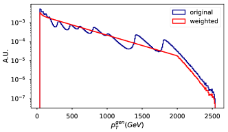
Figure 1: Distribution of the jet transverse momentum at particle level for the hadronic jets in the input dataset. The blue histogram shows the distribution as coming from the dataset, while the red one shows the distribution obtained after applying the weights used for training.

Each pair of jet images is further associated to four auxiliary features: the transverse momentum ($p^{gen}_{T}$), pseudo-rapidity ($\eta^{gen}$) and azimuthal angle ($\phi^{gen}$) of the particle-level jet, and the number of pile-up interactions ($n_{PU}$) that were simulated in the event under consideration. No further preprocessing or standardisation was performed on the input data, which is available on the Zenodo information server data .

The distribution of $p^{gen}_{T}$ for the selected hadronic jets is shown by the blue histogram in figure 1. The shape of the distributions is multi-modal because the original dataset was split in several bins in the scale of the parton-parton interaction. A set of weighting factors, as a function of $p^{gen}_{T}$ was applied to obtain a falling distribution. The distribution obtained after applying such weighting factors is shown by the red histogram.

2.1 Notation and learning setup

We adopt the following notation: we denote by $\mathbf{x}$ and $\mathbf{y}$ the jet image at particle and reconstruction level, respectively, we indicate with $\mathbf{c}$ the set of auxiliary features, and we use $\mathbf{z}$ to denote a latent space of uniformly distributed noise. With this notation, our problem can be formulated as follows.

• Given:

  • $(\mathbf{c},\mathbf{x})\sim p_{cx}(\mathbf{c},\mathbf{x})$

  • $\mathbf{y}\sim p_{y}(\mathbf{y}|\mathbf{x},\mathbf{c})$

  • $\mathbf{z}\sim p_{z}(\mathbf{z})=U(\mathbf{z})$;

  where $p_{cx}$ and $p_{y}$ are the input-data distributions, and $U$ indicates the uniform distribution.

• We want to construct a function $G$, such that

  • $\mathbf{y^{\prime}}=G(\mathbf{z},\mathbf{x},\mathbf{c})\sim p_{y}(\mathbf{y^{\prime}}|\mathbf{x},\mathbf{c})$.

We note that the $\mathbf{c}$ and $\mathbf{x}$ variables sets play, from a mathematical point of view, an identical role in the problem, as we want to condition the output of $G$ is conditional on the union of the two. The reason to separate them is mostly conceptual, as $\mathbf{x}$ represents the image data associated with a jet, while $\mathbf{c}$ parametrises information about jet kinematics and the environment. Furthermore, the two sets of variables are treated differently by the neural network architecture, as detailed in the following.

The function $G$ is a generative model that approximates the combined response of particle detector simulation and reconstruction algorithms to hadronic jets. Following the GAN paradigm, we look for a solution to this problem by introducing a discriminative model $D$ and setting-up a minimax game between the two models, with value function $V(G,D)$ defined as:

$$\begin{array}[]{ll}V(G,D)~{}=&\min_{G}\max_{D}\{\mathbb{E}_{(\mathbf{c},\mathbf{x},\mathbf{y})}\left[\log(D(\mathbf{y},\mathbf{x},\mathbf{c}))\right]\\[4.30554pt] &~{}~{}+~{}\mathbb{E}_{(\mathbf{c},\mathbf{x},\mathbf{z})}\left[\log(1-D(G(\mathbf{z},\mathbf{x},\mathbf{c}),\mathbf{x},\mathbf{c}))\right]\large\}\end{array}$$ (1)

While the problem could in principle be solved using the GAN setup alone, we inject additional information in order to stabilise and speed-up the convergence. In particular, we take into account two facts:

1. $G$ and $\mathbf{y}$ should match on average;

2. $\mathbf{y}$ is very sparse (on average, roughly 3% of the pixels have non-zero values).

The authors of pix2pix show that the first requirement can be efficiently satisfied by adding an $L_{2}$- or $L_{1}$-norm term to the loss function. We adopt this approach, using in particular an $L_{2}$-norm term.

To explicitly take into account the second requirement, we modify the structure of the generator, by increasing the depth of its output: one channel is used to model the pixel intensity, while a second channel, to which we refer as a “soft-mask”, models the probability of a pixel to be non-zero. We denote the two channels as $G_{0}$ and $G_{1}$, and we modify the generative model loss function by adding a term of this form:

$$\begin{array}[]{ll}\lambda&{\rm{\cal L}_{P}}(G)~{}=\lambda~{}\mathbb{E}_{\mathbf{y}=0}\left[-\log(G_{0}(\mathbf{z},\mathbf{x},\mathbf{c}))\right]\\ &+~{}\lambda~{}\mathbb{E}_{\mathbf{y}>0}\left[-\log(1-G_{0}(\mathbf{z},\mathbf{x},\mathbf{c}))+\left(G_{1}(\mathbf{z},\mathbf{x},\mathbf{c})-\mathbf{y}\right)^{2}/2\right]\\ \end{array}$$ (2)

where $\lambda$ is the associated hyperparameter.

To generate images, we sample the soft-mask probabilities to create a “hard-mask” binary stochastic layer $G_{1}^{\prime}(\mathbf{z})=\mathbf{1}_{\mathbf{z}<G_{1}}$, where $\mathbf{1}$ is the so-called indicator function. The GAN value function in eq. 4 becomes $V(G_{2},D)$, where $G_{2}$ is defined as $G_{0}\cdot G_{1}^{\prime}$, and the differentiability is preserved by replacing $G_{1}^{\prime}$ with $G_{1}$ during back-propagation hinton_bsn .

Finally, we enforce a good modelling of the total image intensity, which is proportional to the reconstructed jet energy, with two additions:

• we add an extra term to the generative model loss function, proportional to the mean squared error of the total image intensities:

  $$\tau{\rm{\cal L}_{T}}(G_{2})~{}=\tau~{}\mathbb{E}\left[\left(I(G_{2}(\mathbf{z},\mathbf{x},\mathbf{c}))-I(\mathbf{y})\right)^{2}\right]$$ (3)

  where the operator $I$ computes the total intensity of the jet images and $\mu$ is the associated hyperparameter.

• We introduce a second discriminative model $D_{T}$ that receives as input the total reconstructed jet image intensities, and the auxiliary features $\mathbf{c}$, and we set-up an additional minimax game, whose importance is controlled by the $\mu$ hyperparameter, with value function $V_{T}(G_{2},D_{T})$, defined as below:

  $$\begin{array}[]{ll}\mu&V_{T}(G_{2},D_{T})=\\[4.30554pt] &\mu\min_{G_{2}}\max_{D_{T}}\{\mathbb{E}\left[\log(D_{T}(I(\mathbf{y}),I(\mathbf{x}),\mathbf{c}))\right]\\[4.30554pt] &~{}~{}+~{}\mathbb{E}\left[\log(1-D_{T}(I(G_{2}(\mathbf{z},\mathbf{x},\mathbf{c})),I(\mathbf{x}),\mathbf{c}))\right]\large\}\end{array}$$ (4)

2.2 Model architecture

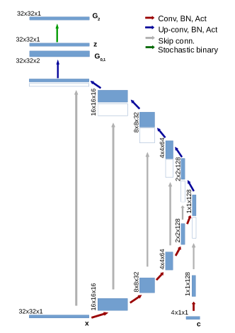
Figure 2: Graphical summary of the generator network. Boxes shows the data representation, while arrows represent operations. Input and output nodes annotated with bold-text labels. On the right side of the diagram, white and blue boxes are concatenated before applying up-convolution operations. Convolutions applied to the $\mathbf{x}$ node and its daughters have a filter size of 3x3, while a 1x1 convolution is applied to the $\mathbf{c}$ node. All up-convolutions use 3x3 filters.

The generative model and the discriminative model $D$ are implemented as convolutional neural networks lecun-98 . For the generator we adopt the so called “U-net” architecture Unet , that consists of an encoding section followed by a decoding one, with additional skip connections linking encoding and decoding layers with the same spatial dimension. The input images are first fed into a batch normalisation layer BN , which allows running the network on non-standardised inputs. Afterwards, we use 5 encoding layers and 5 decoding ones. Each encoding layer consists of a convolutional unit, followed by a batch-normalisation one and by a leaky ReLU activation LReLU , with a slope of 0.2 in the negative domain. The encoding filters size is chosen to be of 3$\times$3, with a stride of 2 in order to reduce the representation width. The number of filters is set to 16 for the first layer and it is doubled at each step. The decoding layers comprise a concatenation unit to implement the skip connections, followed by up-convolutional units, batch normalisation and leaky ReLU activation ones. Drop-out units are also employed in the first two layers of the decoding section. At each step in the decoding section, the depth of the representation is halved, while its width is doubled. This is achieved by decreasing the number of convolutional filters, while appropriately choosing the stride and padding parameters. Auxiliary conditional features are injected in the architecture as follows: they are first passed through a batch normalisation unit and then into a 1$\times$1 convolution unit whose output matches the depth of the last encoding layer; the 1$\times$1 convolutional unit output is subsequently concatenated with that of the last encoding convolution. Noise can be injected into the architecture at the same level. However, we obtained better results by feeding noise only in the form of a stochastic sampling of the output soft-mask. Figure 2 shows a graphical summary of the generator architecture.

The discriminative model $D$ uses 4 layers, comprising 3$\times$3 convolutional filter units, batch normalisation units and leaky ReLU activation ones. Stride and padding are tuned in such a way that the largest field of view of the convolution layers is of 13$\times$13 pixels. The model acts as a “patch-GAN” pix2pix , i.e. it is only sensitive to the local structure of the jet images. The convolutional layers are followed by a fully-connected layer with a sigmoid activation function. The auxiliary variables are treated similarly to what is done in the generative model and are injected at the input of the fully connected layer.

The model $D_{T}$ takes as input the total intensities for $\mathbf{y}$ (or $G_{2}$) as well as $\mathbf{c}$, and is parametrised as a feed-forward fully connected neural network with 4 layers, using dense units, batch normalisation and leaky ReLU activations. The fully connected layers have widths of 64-64-32-16 and are followed by an output layer with a sigmoid activation function.

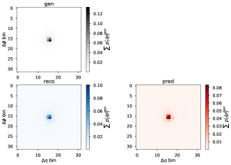
Figure 3: Average jet images obtained at the particle-level (“gen”), after detector simulation and reconstruction (“reco”), and those predicted by the generative model (“pred”).

We did not perform a formal optimisation of the neural networks architecture, but we picked a particular set of values after exploring the parameter space in terms of width and depth of the networks, based on two factors: the performance of the model and the computational times required.

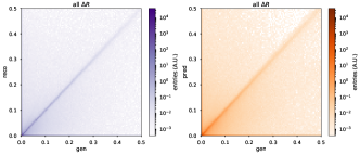
Figure 4: Joint distribution of the particle-level (“gen”) and reconstruction level pixel intensities. The left plot shows the distribution of the input data, while the right plot is obtained using the generative model.

A software package implementing the neural networks’ instantiation and training is openly available in code .

3 Results

The models were trained on two million jet images extracted from the dataset described in section 2. The TensorFlow tf framework, and the Keras keras high level interface were used to implement and train the models. Computing resources from the Piz Daint Cray supercomputer located at the Swiss Centre for Supercomputing were used to obtain the results that we present here. Two independent Adam adam optimisers were employed for parameter sets of the generative and discriminative models. NVIDIA Pascal P100 GPUs were used to accelerate the computations and the models were trained for 10-20 epochs, which were sufficient to achieve convergence. The training time for these models was around 1 hour per epoch. Inference ran at roughly 100Hz on Intel Xeon CPUs and at roughly 10kHz on NVIDIA Pascal P100 GPUs, which are to be compared to the typical time scale for event simulation and reconstruction, i.e. $10^{-1}$–$10^{-2}$ Hz.

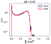
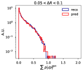
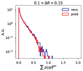
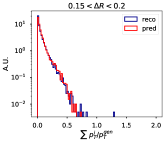
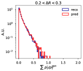
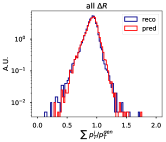
Figure 5: Aggregated pixel intensities for different rings in $\Delta\eta$–$\Delta\phi$. Blue histograms are obtained from the input data, while red ones are obtained using the generative model.

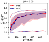
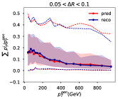
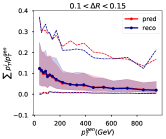
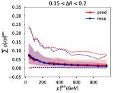
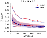
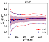
Figure 6: Evolution of the aggregated pixel intensities for different rings in $\Delta\eta$–$\Delta\phi$ as a function of the particle level jet transverse momentum. Solid lines represent the median of the distribution, filled regions show the inter-quartile range, while dashed lines mark the 10% and 90% quantiles. Blue lines are obtained from the input data, while red ones are obtained using the generative model.

Figure 3 shows the average jet image obtained at particle-level by aggregating the $\mathbf{y}$ values, as well as those obtained at reconstruction-level by aggregating either the $\mathbf{x}$ values or the $G_{2}$ ones. One can observe that the average effect of the detector simulation and reconstruction algorithms is to generally spread the jet energy away from the core. We see that this general trend is correctly reproduced by our set-up.

Figure 4 shows the correlation between the particles and detector-level pixel intensities for the input dataset and for the predicted images, obtained from a test sample of 100000 images. Three sub-populations can be observed in the distributions:

• well measured jet components populate the diagonal;

• errors in the position reconstruction of the jet components lead to energy migration between close-by pixels and thus contribute to the sub-populations located close to the horizontal and vertical axes;

• non-reconstructed jet components manifest as empty reconstruction-level pixels that correspond to non-empty ones at particle level and therefore to the sub-population located along the horizontal axis

• pile-up effects lead to non-empty pixels in the reconstruction level image in correspondence to empty particle-level pixels and so contribute to the sub-population close to the vertical axis.

As can be seen from the figure, our set-up (right panel) achieves a good modelling of the relative weight of the three sub-populations, which result from a non-trivial set of effects. The sub-populations located along the diagonal, the horizontal axis and the vertical one account for about 40%, 25% and 25% of the non-empty pixels, respectively and our algorithm is able to reproduce such numbers with a relative accuracy of roughly 30%.

In figure 5 we show the distributions of the total pixel intensities obtained integrating over rings in $\Delta R$ centred on the particle-level jets axis. Blue histograms are obtained from the input dataset, while red ones show the results of the generative model. Figure 6 shows the evolution of the aggregated pixel intensities distribution as a function of the particle-level jet transverse momentum. These results show that our set-up allows good modelling of hadronic jet structure over more than two orders of magnitude in jet transverse momentum.

We further investigate the goodness of the learned model by evaluating its ability to reproduce high level jet features that are typically used in physics analyses. We concentrate, in particular on two sets of variables:

1. variables used in the context of quark/gluon discrimination;

2. jet substructure variables used in the context of merged jets discrimination.

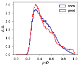
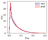
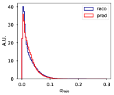
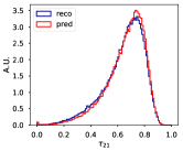
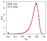
Figure 7: Distribution of high level variables used for quark/gluon discrimination (first two rows) and merged jets tagging (last row). Blue histograms are obtained from the input data, while red ones are obtained using the generative model.

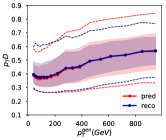
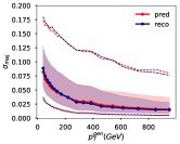
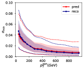
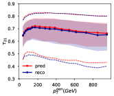
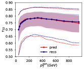
Figure 8: Evolution of the quark/gluon (first two rows) discrimination and merged jet tagging (last row) variables as a function of the particle level jet transverse momentum. Solid lines represent the median of the distribution, filled regions show the inter-quartile range, while dashed lines mark the 10% and 90% quantiles. Blue lines are obtained from the input data, while red ones are obtained using the generative model.

From the first set, we choose the so-called major and minor axes, i.e. the square root of the eigenvalues of the $\eta$-$\phi$ covariance matrix of the jet image, and the $p_{T}D$ variable, i.e. the ratio between the square root of the second and first non-central moment of the pixel intensities Pandolfi2013 . From the second set, we choose the ratio between the 2- and 1-subjettines subjett and that between the 2- and 3-subjettiness. The subjettiness variables were computed using the FastJet package fastjet1 ; fastjet2 , approximating each jet as a set of mass-less particles with energies and directions obtained from the pixel intensities and positions.

Figure 7 shows the distribution of the quark/gluon and merged jets discrimination variables that we considered aggregated over the test dataset, while figure 8 shows the evolution of the distributions as a function of the transverse momentum of the jet at particle level. The level at which these variables are predicted by our set-up is good (in general, the marginal densities and the value of the distributions quantiles are predicted with an accuracy of 5-10%), even though some mismodelling can be observed for the quark-gluon discriminating variables. In particular, mismodelling at the 10-20% level in the marginal density, and in the $p^{gen}_{T}$ dependence of the 75% and 90% quantiles can be observed for the $p_{T}D$ and the major and minor axes. These kind of disagreements point to the fact that the correlation between the number of non-empty pixels and their energy sharing is not perfectly modelled.

3.1 Discussion

The results that we discussed above represent a step forward in terms of accuracy of fast simulation systems proposed in the context of collider detector physics. We believe that three main aspects contributed to this:

• the use of a generative model that is designed to handle spatial correlations well, and the use of a conditioning space (i.e. that of particle-level images) that encodes large amounts of spatial information;

• the explicit handling of the sparsity through the soft-mask layer;

• the use of physics-driven constraints on the total intensity of the jet images.

The method that we outline here has potential application in conjunction with fast detector simulation models, or parametrised ones delphes ; cms_fast_sim . In this context, being able to accurately predict the output of simulation and reconstruction algorithms for objects like hadronic jets, which are ubiquitous at the LHC, would allow to save large amounts of the computing power, by reducing the cost of producing simulated events samples.

While a relatively stable set-up was established by tuning the model hyper-parameters, this aspect of the work is not yet completely satisfactory, as the region of hyper-parameters space that lead to satisfactory results was found to be relatively narrow. A review of the loss function structure, possibly incorporating the use of alternative formulations of the GAN game f_gan ; w_gan1 ; w_gan2 , and of the model training strategy in general, will be important to allow streamlining the method, and will the subject of future work.

Furthermore, the current approach introduces noise only through the stochastic generation of the set of active pixels. Our attempts at injecting noise at a more fundamental level in the generative model structure have been unsuccessful so far. Similar problems have been reported by researchers working on natural image generation (see e.g. pix2pix ). A more extensive investigation of the handling of noise will also be subject of subsequent work.

4 Conclusions

We have reported on a method that uses deep neural networks to learn the response of particle detectors simulation and reconstruction algorithms. The method is based on generative adversarial networks and it was applied to the generation of hadronic jet images at the CERN LHC.

We trained a generative model to reproduce the combined response of state-of-the-art simulation and reconstruction algorithms. This was possible thanks to the exploitation of the open datasets published by the CMS collaboration under the HEP data preservation initiative.

Starting from proposals made for natural image processing, we devised a hybrid set-up based on the combined use of generative adversarial networks and analytic loss functions that is able to take into account the conditioning on auxiliary variables and physics-driven constraints on the generation process.

Our method allows reducing the computation time required to obtain reconstruction-level hadronic jets from particle-level jets by several orders of magnitude, while achieving a very good accuracy in reproducing the simulation and reconstruction algorithms response. The model is in particular capable of reproducing the evolution of the reconstructed jet shapes as a function of several conditional variables. Physics-driven high level features commonly used for merged jets tagging and quark/gluon discrimination, and their evolution, are also generally well modelled.

The results obtained with this work represent a promising step forward towards the development of fast and accurate simulation systems that will be crucial for the future of collider experiments in high energy physics.

Conflicts of interest

On behalf of all authors, the corresponding author states that there is no conflict of interest.

Appendix A Comparison with traditional fast simulation methods

In this appendix we compare the results obtained using our generative neural networks with methods for fast simulation traditionally used for phenomenological studies in high energy physics. These packages parametrise particle detectors responses, on a particle by particle basis, in terms of gaussian energy and momentum resolutions and binomial reconstruction probabilities. In particular, we compared the results obtained with our GAN with the output of the DELPHES delphes package. In order to do that, we used version 3.4.1 of the program and the standard CMS datacard included in the package.

In figures 9 and 10 we show the same quantities as shown in figures 5 and 6, respectively, but with the addition of the results obtained with the DELPHES gaussian-smearing model (shown in gray). As can be seen the simple gaussian-smearing approach fails to describe the fine structure of particle jets, and shows that our neural network based approach provides results of superior quality, compared to traditional fast simulation methods.

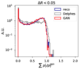
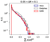
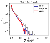
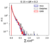
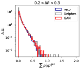
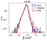
Figure 9: Aggregated pixel intensities for different rings in $\Delta\eta$–$\Delta\phi$. Blue histograms are obtained from the input data; red ones are obtained using the generative model; gray histograms are obtained with a gaussian-smearing model.

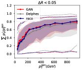
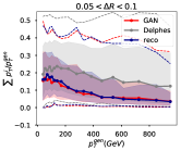
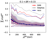
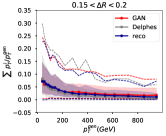
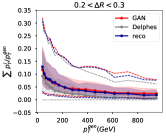
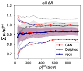
Figure 10: Evolution of the aggregated pixel intensities for different rings in $\Delta\eta$–$\Delta\phi$ as a function of the particle level jet transverse momentum. Solid lines represent the median of the distribution, filled regions show the inter-quartile range, while dashed lines mark the 10% and 90% quantiles. Blue lines are obtained from the input data; red ones are obtained using the generative model; gray ones using the gaussian-smearing model.

Appendix B Differential characterisation of the image translation

In this appendix we report a differential comparison of the jet images obtained at particle level, reconstruction level, and through our generative model. In figures 11 and 12 we show the same quantities as shown in figures 5 and 6, respectively, but with the addition of results obtained using particle level jets.

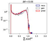
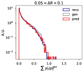
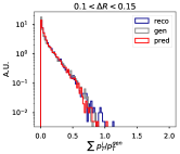
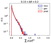
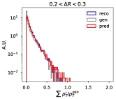
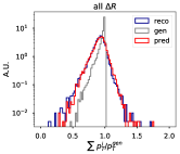
Figure 11: Aggregated pixel intensities for different rings in $\Delta\eta$–$\Delta\phi$. Blue histograms are obtained from the full simulation and reconstruction chain; red ones are obtained using the generative model; gray histograms show the quantities obtained before detector simulation.

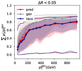
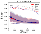
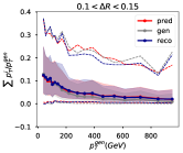
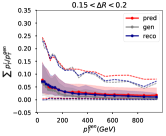
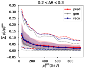
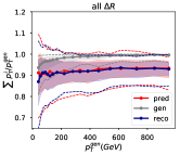
Figure 12: Evolution of the aggregated pixel intensities for different rings in $\Delta\eta$–$\Delta\phi$ as a function of the particle level jet transverse momentum. Solid lines represent the median of the distribution, filled regions show the inter-quartile range, while dashed lines mark the 10% and 90% quantiles. Blue histograms are obtained from the full simulation and reconstruction chain; red ones are obtained using the generative model; gray histograms show the quantities obtained before detector simulation.

References

- (1) S. Agostinelli, et al., Geant4-a simulation toolkit, Nuclear Instruments and Methods in Physics Research Section A 506(3), 250 (2003). DOI 10.1016/S0168-9002(03)01368-8
- (2) G. Aad, et al., The ATLAS Experiment at the CERN Large Hadron Collider, JINST 3, S08003 (2008). DOI 10.1088/1748-0221/3/08/S08003
- (3) S. Chatrchyan, et al., The CMS Experiment at the CERN LHC, JINST 3, S08004 (2008). DOI 10.1088/1748-0221/3/08/S08004
- (4) G. Apollinari, et al., High-Luminosity Large Hadron Collider (HL-LHC) (2017). DOI 10.23731/CYRM-2017-004
- (5) A.A. Alves, Jr, et al., A Roadmap for HEP Software and Computing R&D for the 2020s. Tech. rep. (2017). URL https://arxiv.org/abs/1712.06982
- (6) /QCD_Pt-30to50_TuneZ2_7TeV_pythia6/Summer11LegDRPU_S13_START53_LV6-v1/AODSIM. DOI 10.7483\/OPENDATA.CMS.Q3BX.69VQ
- (7) /QCD_Pt-50to80_TuneZ2_7TeV_pythia6/Summer11LegDRPU_S13_START53_LV6-v1/AODSIM. DOI 10.7483\/OPENDATA.CMS.84VC.RU8W
- (8) /QCD_Pt-80to120_TuneZ2_7TeV_pythia6/Summer11LegDRPU_S13_START53_LV6-v1/AODSIM. DOI 10.7483\/OPENDATA.CMS.PUTE.7H2H
- (9) /QCD_Pt-120to170_TuneZ2_7TeV_pythia6/Summer11LegDRPU_S13_START53_LV6-v1/AODSIM. DOI 10.7483\/OPENDATA.CMS.QJND.HA88
- (10) /QCD_Pt-170to300_TuneZ2_7TeV_pythia6/Summer11LegDRPU_S13_START53_LV6-v1/AODSIM. DOI 10.7483\/OPENDATA.CMS.WKRR.DCJP
- (11) /QCD_Pt-300to470_TuneZ2_7TeV_pythia6/Summer11LegDRPU_S13_START53_LV6-v1/AODSIM. DOI 10.7483\/OPENDATA.CMS.X3XQ.USQR
- (12) /QCD_Pt-470to600_TuneZ2_7TeV_pythia6/Summer11LegDRPU_S13_START53_LV6-v1/AODSIM. DOI 10.7483\/OPENDATA.CMS.BKTD.SGJX
- (13) /QCD_Pt-600to800_TuneZ2_7TeV_pythia6/Summer11LegDRPU_S13_START53_LV6-v1/AODSIM. DOI 10.7483\/OPENDATA.CMS.EJT7.KSAY
- (14) /QCD_Pt-800to1000_TuneZ2_7TeV_pythia6/Summer11LegDRPU_S13_START53_LV6-v1/AODSIM. DOI 10.7483\/OPENDATA.CMS.S3D5.KF2C
- (15) /QCD_Pt-1000to1400_TuneZ2_7TeV_pythia6/Summer11LegDRPU_S13_START53_LV6-v1/AODSIM. DOI 10.7483\/OPENDATA.CMS.96U2.3YAH
- (16) /QCD_Pt-1400to1800_TuneZ2_7TeV_pythia6/Summer11LegDRPU_S13_START53_LV6-v1/AODSIM. DOI 10.7483\/OPENDATA.CMS.RC9V.B5KX
- (17) /QCD_Pt-1800_TuneZ2_7TeV_pythia6/Summer11LegDRPU_S13_START53_LV6-v1/AODSIM. DOI 10.7483\/OPENDATA.CMS.CX2X.J3KW
- (18) R. Mount, et al., Data Preservation in High Energy Physics, Intermediate report of the ICFA-DPHEP Study Group (2009). URL https://arxiv.org/abs/0912.0255
- (19) I.J. Goodfellow, J. Pouget-Abadie, M. Mirza, B. Xu, D. Warde-Farley, S. Ozair, A. Courville, Y. Bengio, Generative Adversarial Networks (2014). URL https://arxiv.org/abs/1406.2661
- (20) S. Arora, R. Ge, Y. Liang, T. Ma, Y. Zhang, in Proceedings of the 34th International Conference on Machine Learning, Proceedings of Machine Learning Research, vol. 70, ed. by D. Precup, Y.W. Teh (PMLR, International Convention Centre, Sydney, Australia, 2017), Proceedings of Machine Learning Research, vol. 70, pp. 224–232. URL http://proceedings.mlr.press/v70/arora17a.html
- (21) S. Nowozin, B. Cseke, R. Tomioka, f-GAN: Training Generative Neural Samplers using Variational Divergence Minimization (2016). URL https://arxiv.org/abs/1606.00709
- (22) I. Gulrajani, F. Ahmed, M. Arjovsky, V. Dumoulin, A.C. Courville, Improved training of wasserstein gans, CoRR abs/1704.00028 (2017). URL http://arxiv.org/abs/1704.00028
- (23) M. Arjovsky, S. Chintala, L. Bottou, Wasserstein GAN (2017). URL https://arxiv.org/abs/1701.07875
- (24) G. Louppe, M. Kagan, K. Cranmer, Learning to pivot with adversarial networks (2016). URL https://arxiv.org/abs/1611.01046
- (25) C. Shimmin, P. Sadowski, P. Baldi, E. Weik, D. Whiteson, E. Goul, A. Søgaard, Decorrelated Jet Substructure Tagging using Adversarial Neural Networks, Phys. Rev. D96(7), 074034 (2017). DOI 10.1103/PhysRevD.96.074034
- (26) V. Estrade, et al., in NIPS 2017 - workshop Deep Learning for Physical Sciences (Long Beach, United States, 2017), pp. 1–5
- (27) L. de Oliveira, M. Paganini, B. Nachman, Learning Particle Physics by Example: Location-Aware Generative Adversarial Networks for Physics Synthesis, Comput. Softw. Big Sci. 1(1), 4 (2017). DOI 10.1007/s41781-017-0004-6
- (28) M. Paganini, L. de Oliveira, B. Nachman, Accelerating Science with Generative Adversarial Networks: An Application to 3D Particle Showers in Multilayer Calorimeters, Phys. Rev. Lett. 120(4), 042003 (2018). DOI 10.1103/PhysRevLett.120.042003
- (29) F. Carminati, et al., in NIPS 2017 - workshop Deep Learning for Physical Sciences (Long Beach, United States, 2017), pp. 1–5
- (30) M. Erdmann, L. Geiger, J. Glombitza, D. Schmidt, Generating and refining particle detector simulations using the Wasserstein distance in adversarial networks (2018). URL https://arxiv.org/abs/1802.03325
- (31) P. Isola, J. Zhu, T. Zhou, A.A. Efros, Image-to-image translation with conditional adversarial networks, CoRR abs/1611.07004 (2016). URL http://arxiv.org/abs/1611.07004
- (32) T. Salimans, I.J. Goodfellow, W. Zaremba, V. Cheung, A. Radford, X. Chen, Improved techniques for training gans, CoRR abs/1606.03498 (2016). URL http://arxiv.org/abs/1606.03498
- (33) M. Mirza, S. Osindero, Conditional generative adversarial nets, CoRR abs/1411.1784 (2014). URL http://arxiv.org/abs/1411.1784
- (34) L. de Oliveira, M. Paganini, B. Nachman, in 18th International Workshop on Advanced Computing and Analysis Techniques in Physics Research (ACAT 2017) Seattle, WA, USA, August 21-25, 2017 (2017)
- (35) J. de Favereau, C. Delaere, P. Demin, A. Giammanco, V. Lemaître, A. Mertens, M. Selvaggi, DELPHES 3, A modular framework for fast simulation of a generic collider experiment, JHEP 02, 057 (2014). DOI 10.1007/JHEP02(2014)057
- (36) T. Sjostrand, S. Mrenna, P.Z. Skands, PYTHIA 6.4 Physics and Manual, JHEP 05, 026 (2006). DOI 10.1088/1126-6708/2006/05/026
- (37) M. Cacciari, G.P. Salam, G. Soyez, The anti- k t jet clustering algorithm, Journal of High Energy Physics 2008(04), 063 (2008). URL http://stacks.iop.org/1126-6708/2008/i=04/a=063
- (38) M. Cacciari, G.P. Salam, G. Soyez, FastJet User Manual, Eur. Phys. J. C72, 1896 (2012). DOI 10.1140/epjc/s10052-012-1896-2
- (39) The data used in this work is available through the following electronic reference. DOI 10.5281/zenodo.1467678. URL http://doi.org/10.5281/zenodo.1467678
- (40) H. Geoffry, et al. Neural networks for machine learning. www.coursera.org
- (41) Y. LeCun, L. Bottou, Y. Bengio, P. Haffner, Gradient-based learning applied to document recognition, Proceedings of the IEEE 86(11), 2278 (1998)
- (42) O. Ronneberger, P. Fischer, T. Brox, U-net: Convolutional networks for biomedical image segmentation, CoRR abs/1505.04597 (2015). URL http://arxiv.org/abs/1505.04597
- (43) S. Ioffe, C. Szegedy, Batch normalization: Accelerating deep network training by reducing internal covariate shift, CoRR abs/1502.03167 (2015). URL http://arxiv.org/abs/1502.03167
- (44) A.L. Maas, A.Y. Hannun, A.Y. Ng, in Proc. icml, vol. 30 (2013), vol. 30, p. 3
- (45) A software package related to this work is available through the following electronic reference. DOI 10.5281/zenodo.1467665. URL http://doi.org/10.5281/zenodo.1467665
- (46) M. Abadi, P. Barham, J. Chen, Z. Chen, A. Davis, J. Dean, M. Devin, S. Ghemawat, G. Irving, M. Isard, M. Kudlur, J. Levenberg, R. Monga, S. Moore, D.G. Murray, B. Steiner, P.A. Tucker, V. Vasudevan, P. Warden, M. Wicke, Y. Yu, X. Zhang, Tensorflow: A system for large-scale machine learning, CoRR abs/1605.08695 (2016). URL http://arxiv.org/abs/1605.08695
- (47) F. Chollet, et al. Keras. https://keras.io (2015)
- (48) D.P. Kingma, J. Ba, Adam: A method for stochastic optimization, CoRR abs/1412.6980 (2014). URL http://arxiv.org/abs/1412.6980
- (49) F. Pandolfi, Search for the Standard Model Higgs boson in the H ZZ decay channel at CMS on 4.6 fb-1 of 7 TeV proton-proton collision data, The European Physical Journal Plus 128(10), 117 (2013). DOI 10.1140/epjp/i2013-13117-x
- (50) J. Thaler, K. Van Tilburg, Identifying boosted objects with n-subjettiness, Journal of High Energy Physics 2011(3), 15 (2011). DOI 10.1007/JHEP03(2011)015
- (51) M. Cacciari, G.P. Salam, G. Soyez, FastJet User Manual, Eur. Phys. J. C72, 1896 (2012). DOI 10.1140/epjc/s10052-012-1896-2
- (52) M. Cacciari, G.P. Salam, Dispelling the myth for the jet-finder, Phys. Lett. B641, 57 (2006). DOI 10.1016/j.physletb.2006.08.037
- (53) R. Rahmat, R. Kroeger, A. Giammanco, The fast simulation of the cms experiment, Journal of Physics: Conference Series 396(6), 062016. DOI 10.1088/1742-6596/396/6/062016