Optimal and Robust Controller Synthesis

Abstract

In this paper, we propose a novel framework for the synthesis of robust and optimal energy-aware controllers. The framework is based on energy timed automata, allowing for easy expression of timing constraints and variable energy rates. We prove decidability of the energy-constrained infinite-run problem in settings with both certainty and uncertainty of the energy rates. We also consider the optimization problem of identifying the minimal upper bound that will permit existence of energy-constrained infinite runs. Our algorithms are based on quantifier elimination for linear real arithmetic. Using Mathematica and Mjollnir, we illustrate our framework through a real industrial example of a hydraulic oil pump. Compared with previous approaches our method is completely automated and provides improved results.

1 Introduction

Design of controllers for embedded systems is a difficult engineering task. Controllers must ensure a variety of safety properties as well as optimality with respect to given performance properties. Also, for several systems, e.g. [8, 27, 25], the properties involve non-functional aspects such as time and energy.

We provide a novel framework for automatic synthesis of safe and optimal controllers for resource-aware systems based on energy timed automata. Synthesis of controllers is obtained by solving time- and energy-constrained infinite run problems. Energy timed automata [12] extend timed automata [2] with a continuous energy variable that evolves with varying rates and discrete updates during the behaviour of the model. Closing an open problem from [12], we prove decidability of the infinite run problem in settings, where rates and updates may be both positive and negative and possibly subject to uncertainty. Additionally, the accumulated energy may be subject to lower and upper bounds reflecting constraints on capacity. Also we consider the optimization problems of identifying minimal upper bounds that will permit the existence of infinite energy-constrained runs. Our decision and optimization algorithms for the energy-constrained infinite run problems are based on reductions to quantifier elimination (QE) for linear real arithmetic, for which we combine Mathematica [28] and Mjollnir [24] into a tool chain.

(a) System Components

(b) Cycle of the Machine

Figure 1: Overview of the HYDAC system

To demonstrate the applicability of our framework, we revisit an industrial case study provided by the HYDAC company in the context of the European project Quasimodo [26]. It consists in an on/off control system (see Fig. 1(a)) composed of (i) a machine that consumes oil according to a cyclic pattern of 20 s (see Fig. 1(b)), (ii) an accumulator containing oil and a fixed amount of gas in order to put the oil under pressure, and (iii) a controllable pump which can pump oil into the accumulator with rate 2.2 l/s. The control objective for switching the pump on and off is twofold: first the level of oil in the accumulator (and so the gas pressure) shall be maintained within a safe interval; second, the controller should try to minimize the (maximum and average) level of oil such that the pressure in the system is kept minimal. We show how to model this system, with varying constraints on pump operation, as energy timed automata. Thus our tool chain may automatically synthesize guaranteed safe and optimal control strategies.

The HYDAC case was first considered in [16] as a timed game using the tool Uppaal-Tiga [15, 5] for synthesis. Discretization of oil-level (and time) was used to make synthesis feasible. Besides limiting the opportunity of optimality, the discretization also necessitated posterior verification using PHAVER [20] to rule out possible resulting incorrectness. Also, identification of safety and minimal oil levels were done by manual and laborious search. In [23] the timed game models of [16] (rephrased as Timed Discrete Event Systems) are reused, but BDDs are applied for compact representation of the discrete oil-levels and time-points encountered during synthesis. [21] provides a framework for learning optimal switching strategies by a combination of off-the-shelf numerical optimization and generalization by learning. The HYDAC case is one of the considered cases. The method offers no absolute guarantees of hard constraints on energy-level, but rather attempts to enforce these through the use of high penalties. [29] focuses exclusively on the HYDAC case using a direct encoding of the safety- and optimality-constraints as QE problems. This gives—like in our case—absolute guarantees. However, we are additionally offering a complete and decidable framework based on energy timed automata, which extends to several other systems. Moreover, the controllers we obtain perform significantly better than those of [16] and [29] (respectively up to 22% and 16% better) and are obtained automatically by our tool chain combining Mjollnir and Mathematica. This combination permits quantifier elimination and formula simplification to be done in a compositional manner, resulting in performance surpassing each tool individually. We believe that this shows that our framework has a level of maturity that meets the complexity of several relevant industrial control problems.

Our work is related to controllability of (constrained) piecewise affine (PWA) [7] and hybrid systems [1]. In particular, the energy-constrained infinite-run problem is related to the so called stability problem for PWAs. Blondel and Tsitsiklis [10] have shown that verifying stability of autonomous piecewise-linear (PWL) systems is -hard, even in the simple case of two-component subsystems; several global properties (e.g. global convergence, asymptotic stability and mortality) of PWA systems have been shown undecidable in [9].

2 Energy Timed Automata

2.0.1 Definitions.

Given a finite set $X$ of clocks, the set of closed clock constraints over $X$, denoted $C(X)$, is the set of formulas built using $g\coloncolonequals x\sim n\mid g\wedge g$, where $x$ ranges over $X$, $\mathord{\sim}$ ranges over $\{\mathord{\leq},\mathord{\geq}\}$ and $n$ ranges over $+$. That a clock valuation $v\colon X\to+$ satisfies a clock constraint $g$, denoted $v\models g$, is defined in the natural way. For a clock valuation $v$, a real $t\in+$, and a subset $R\subseteq X$, we write $v+t$ for the valuation mapping each clock $x\in X$ to $v(x)+t$, and $v[R\to 0]$ for the valuation mapping clocks in $R$ to zero and clocks not in $R$ to their value in $v$. Finally we write $\mathbf{0}_{X}$ (or simply $\mathbf{0}$) for the clock valuation assigning $0$ to every $x\in X$.

For $E\subseteq$, we let $(E)$ be the set of closed intervals of  with bounds in $E\cap$. Notice that any interval in $(E)$ is bounded, for any $E\subseteq$.

Definition 1

An energy timed automaton (ETA for short; a.k.a. priced or weighted timed automaton [3, 6]) is a tuple $=(\penalty 10000S,S_{0},\penalty-1000X,\penalty-1000I,\penalty-1000r,T\penalty 10000)$ where $S$ is a finite set of states, $S_{0}\subseteq S$ is the set of initial states, $X$ is a finite set of clocks, $I\colon S\to C(X)$ assigns invariants to states, $r\colon S\to$ assigns rates to states, and $T\subseteq S\times C(X)\times\times 2^{X}\times S$ is a finite set of transitions.

An energy timed path (ETP, a.k.a. linear energy timed automaton) is an energy timed automaton for which $S$ can be written as $\{s_{i}\mid 0\leq i\leq n\}$ in such a way that $S_{0}=\{s_{0}\}$, and $T=\{(s_{i},g_{i},u_{i},z_{i},s_{i+1})\mid 0\leq i<n\}$. We additionally require that all clocks are reset on the last transition, i.e., $z_{n-1}=X$.

Let $=(\penalty 10000S,S_{0},\penalty-1000X,\penalty-1000I,\penalty-1000r,T\penalty 10000)$ be an ETA. A configuration of is a triple $(\ell,v,w)\in S\times(+)^{X}\times$, where $v$ is a clock valuation, and $w$ is the energy level. Let $\tau=(t_{i})_{0\leq i<n}$ be a finite sequence of transitions, with $t_{i}=(s_{i},g_{i},u_{i},z_{i},s_{i+1})$ for every $i$. A finite run in on $\tau$ is a sequence of configurations $\rho=(\ell_{j},v_{j},w_{j})_{0\leq j\leq 2n}$ such that there exists a sequence of delays $(d_{i})_{0\leq i<n}$ for which the following requirements hold:

• for all $0\leq j<n$, $\ell_{2j}=\ell_{2j+1}=s_{j}$, and $\ell_{2n}=s_{n}$;

• for all $0\leq j<n$, $v_{2j+1}=v_{2j}+d_{j}$ and $v_{2j+2}=v_{2j+1}[z_{j}\to 0]$;

• for all $0\leq j<n$, $v_{2j}\models I(s_{j})$ and $v_{2j+1}\models I(s_{j})\wedge g_{j}$;

• for all $0\leq j<n$, $w_{2j+1}=w_{2j}+d_{j}\cdot r(s_{j})$ and $w_{2j+2}=w_{2j+1}+u_{j}$.

We will by extension speak of runs read on ETPs (those runs will then end with clock valuation $\mathbf{0}$). The notion of infinite run is defined similarly. Given $E\in()$, such a run is said to satisfy energy constraint $E$ if $w_{j}\in E$ for all $j$.

Example 1

Fig. 2 displays an example of an ETP  and one of its runs $\rho$. Since no time will be spent in $s_{2}$, we did not indicate the invariant and rate of that state. The sequence $\rho$ is a run of . Spending $0.6$ time units in $s_{0}$, the value of clock $x$ reaches $0.6$, and the energy level grows to ${3+0.6\times 2=4.2}$; it equals ${4.2-3=1.2}$ when entering $s_{1}$. Then $\rho$ satisfies energy constraint $[0;5]$.

Figure 2: An energy timed path , and a run $\rho$ of  with initial energy level $3$.

Definition 2

A segmented energy timed automaton (SETA for short) is a tuple $=(\penalty 10000S,T,P\penalty 10000)$ where $(\penalty 10000S,T\penalty 10000)$ is a finite graph (whose states and transitions are called macro-states and macro-transitions), $S_{0}$ is a set of initial macro-states, and $P$ associates with each macro-transition $t=(s,s^{\prime})$ of  an ETP with initial state $s$ and final state $s^{\prime}$. We require that for any two different transitions $t$ and $t^{\prime}$ of , the state spaces of $P(t)$ and $P(t^{\prime})$ are disjoint and contain no macro-states, except (for both conditions) for their first and last states.

A SETA is flat if the underlying graph $(\penalty 10000S,T\penalty 10000)$ is (i.e., for any $s\in S$, there is at most one non-empty path in the graph $(\penalty 10000S,T\penalty 10000)$ from $s$ to itself [17, 14]). It is called depth-1 whenever the graph $(\penalty 10000S,T\penalty 10000)$ is tree-like, with only loops at leaves.

A (finite or infinite) execution of a SETA is a (finite or infinite) sequence of runs $\rho=(\rho^{i})_{i}$ such that for all $i$, writing $\rho^{i}=(\ell^{i}_{j},v^{i}_{j},w^{i}_{j})_{0\leq j\leq 2n_{i}}$, it holds:

• $\ell^{i}_{0}$ and $\ell^{i}_{2n_{i}}$ are macro-states of , and $\rho^{i}$ is a run of the ETP $P(\ell^{i}_{0},\ell^{i}_{2n_{i}})$;

• $\ell^{i+1}_{0}=\ell^{i}_{2n_{i}}$ and $w^{i+1}_{0}=w^{i}_{2n_{i}}$.

Hence a run in a SETA should be seen as the concatenation of paths $\rho^{i}$ between macro-states. Notice also that each $\rho^{i}$ starts and ends with all clock values zero, since all clocks are reset at the end of each ETP, when a main state is entered. Finally, given an interval $E\in()$, an execution $(\rho^{i})_{i}$ satisfies energy constraint $E$ whenever all individual runs $\rho^{i}$ do.

Remark 1

In contrast with ETAs, the class of SETAs is not closed under parallel composition. Intuitively, the ETA resulting from the parallel composition of two SETAs may not be “segmented” into a graph of energy timed-paths because the requirement that all clocks are reset on the last transition may not be satisfied. Furthermore, parallel composition does not preserve flatness because it may introduce nested loops.

Example 2

Figure 3 displays a SETA  with two macro-states $s_{0}$ and $s_{2}$, and two macro-transitions. The macro-self-loop on $s_{2}$ is associated with the energy timed path of Fig. 2. The execution $\rho=\rho^{1}\cdot(\rho^{2}\cdot\rho^{3})^{\omega}$ is an ultimately-periodic execution of . This infinite execution satisfies the energy constraint $E=[0;5]$ (as well as the (tight) energy constraint $[1;4.6]$).

Figure 3: A SETA $=(\penalty 10000S,T,P\penalty 10000)$ with implicit global invariant $y\leq 1$; omitted discrete updates are assumed to be zero. The map $P$ associates with each $(s_{i},s_{j})\in T$ the ETP $P_{i,j}$. The infinite sequence $\rho^{1}\cdot(\rho^{2}\cdot\rho^{3})^{\omega}$ is an infinite execution of  with initial energy level $3$ satisfying the energy constraint $E=[0;5]$.

In this paper, we consider the following energy-constrained infinite-run problem [12]: given an energy timed automaton  and a designated state $s_{0}$, an energy constraint $E\in()$ and an initial energy level $w_{0}\in E$, does there exist an infinite execution in  starting from $(s_{0},\mathbf{0},w_{0})$ that satisfies $E$?

In the general case, the energy-constrained infinite-run problem is undecidable, even when considering ETA with only two clocks [22]. In this paper, we prove:

Theorem 2.3 ()

The energy-constrained infinite-run problem is decidable for flat SETA.

Theorem 2.4 ()

Given a fixed lower bound $L$, the existence of an upper bound $U$, such that there is a solution to the energy-constrained infinite-run problem for energy constraint $E=[L;U]$, is decidable for flat SETA. If such a $U$ exists, then for depth-1 flat SETA, we can compute the least one.

We only sketch a proof of the former result, and refer to [4] for the full proof.

2.0.2 Binary energy relations.

Let $=(\penalty 10000\{s_{i}\mid 0\leq i\leq n\},\{s_{0}\},\penalty-1000X,\penalty-1000I,\penalty-1000r,T\penalty 10000)$ be an ETP from $s_{0}$ to $s_{n}$. Let $E\subseteq()$ be an energy constraint. The binary energy relation ${}_{{}^{E}}\subseteq E\times E$ for  under energy constraint $E$ relates all pairs $(w_{0},w_{1})$ for which there is a finite run of  from $(s_{0},\mathbf{0},w_{0})$ to $(s_{n},\mathbf{0},w_{1})$ satisfying energy constraint $E$. This relation is characterized by the following first-order formula:

$${}_{{}^{E}}(w_{0},w_{1})\iff\exists(d_{i})_{0\leq i<n}.\ \Phi_{\text{timing}}\wedge\Phi_{\text{energy}}\wedge w_{1}=w_{0}+\sum_{k=0}^{n-1}(d_{k}\cdot r(s_{k})+u_{k})$$

where $\Phi_{\text{timing}}$ encodes all the timing constraints that the sequence $(d_{i})_{0\leq i<n}$ has to fulfill (derived from guards and invariants, by expressing the values of the clocks in terms of $(d_{i})_{0\leq i<n}$), while $\Phi_{\text{energy}}$ encodes the energy constraints (in each state, the accumulated energy must be in $E$).

It is easily shown that ${}_{P}^{E}$ is a closed, convex subset of $E\times E$ (remember that we consider closed clock constraints); thus it can be described as a conjunction of a finite set of linear constraints over $w_{0}$ and $w_{1}$ (with non-strict inequalities), using quantifier elimination of variables $(d_{i})_{0\leq i<n}$.

Example 3

We illustrate this computation on the ETP of Fig. 2. For energy constraint $[0;5]$, the energy relation (after removing redundant constraints) reads as

$${}_{{}^{E}}(w_{0},w_{1})\iff\exists d_{0},d_{1}.\ d_{0}\in[0.25;1]\wedge d_{1}\in[0;1]\wedge d_{0}+d_{1}=1\wedge{}$$

$$w_{0}\in[0;5]\wedge w_{0}+2d_{0}\in[0;5]\wedge w_{0}+2d_{0}-3\in[0;5]\wedge{}$$

$$w_{1}=w_{0}+2d_{0}+4d_{1}-3\wedge w_{1}\in[0;5].$$

This simplifies to $(w_{1}+2\leq 2w_{0}\leq w_{1}+4)\wedge(w_{1}-0.5\leq w_{0}\leq w_{1}+1)$. The corresponding polyhedron is depicted above.

2.0.3 Energy functions.

We now focus on properties of energy relations. First notice that for any interval $E\in()$, the partially-ordered set $((E),\supseteq)$ is $\omega$-complete, meaning that for any chain $(I_{j})_{j\in}$, with $I_{j}\supseteq I_{j+1}$ for all $j$, the limit $\bigcap_{j\in}I_{j}$ also belongs to $(E)$. By Cantor’s Intersection Theorem, if additionally each interval $I_{j}$ is non-empty, then so is the limit $\bigcap_{j\in}I_{j}$.

With an energy relation ${}_{{}^{E}}$, we associate an energy function (also denoted with ${}_{{}^{E}}$, or simply , as long as no ambiguity may arise), defined for any closed sub-interval $I\in(E)$ as $(I)=\{w_{1}\in E\mid\exists w_{0}\in I.\ (w_{0},w_{1})\}$. Symmetrically:

$${}^{-1}(I)=\{w_{0}\in E\mid\exists w_{1}\in I.\ (w_{0},w_{1})\}.$$

Observe that $(I)$ and ${}^{-1}(I)$ also belong to $(E)$ (because the relation  is closed and convex). Moreover, and ^-1 are non-decreasing: for any two intervals $I$ and $J$ in $(E)$ such that $I\subseteq J$, it holds $(I)\subseteq(J)$ and ${}^{-1}(I)\subseteq^{-1}(J)$. Energy function ^-1 also satisfies the following continuity property:

Lemma 5 ()

Let $(I_{j})_{j\in}$ be a chain of intervals of $(E)$, such that $I_{j}\supseteq I_{j+1}$ for all $j\in$. Then ${}^{-1}(\bigcap_{j\in}I_{j})=\bigcap_{j\in}^{-1}(I_{j})$.

2.0.4 Composition and fixpoints of energy functions.

Consider a finite sequence of paths $(_{i})_{1\leq i\leq k}$. Clearly, the energy relation for this sequence can be obtained as the composition of the individual energy relations ${}_{{}_{k}}^{E}\circ\cdots\circ_{{}_{1}}^{E}$; the resulting energy relation still is a closed convex subset of $E\times E$ that can be described as the conjunction of finitely many linear constraints over $w_{0}$ and $w_{1}$. As a special case, we write $(_{^{E}})^{k}$ for the composition of $k$ copies of the same relations ${}_{{}^{E}}$.

Now, using Lemma 5, we easily prove that the greatest fixpoint $\nu^{-1}$ of ^-1 in the complete lattice $((E),\supseteq)$ exists and equals:

$$\nu^{-1}=\bigcap_{i\in}(^{-1})^{i}(E).$$

Moreover $\nu^{-1}$ is a closed (possibly empty) interval. Note that $\nu^{-1}$ is the maximum subset $S$ of $E$ such that, starting with any $w_{0}\in S$, it is possible to iterate  infinitely many times (that is, for any $w_{0}\in S$, there exists $w_{1}\in S$ such that $(w_{0},w_{1})$—any such set $S$ is a post-fixpoint of ^-1, i.e. $S\subseteq^{-1}(S)$).

If is the energy relation of a cycle  in the flat SETA, then $\nu^{-1}$ precisely describes the set of initial energy levels allowing infinite runs through  satisfying the energy constraint $E$. If  is described as the conjunction $\phi$ of a finite set of linear constraints, then we can characterize those intervals $[a,b]\subseteq E$ that constitute a post-fixpoint for ^-1 by the following first-order formula:

$$a\leq b\wedge a\in E\wedge b\in E\wedge\forall w_{0}\in[a;b].\ \exists w_{1}\in[a;b].\ \phi_{(}w_{0},w_{1}).$$ (1)

Applying quantifier elimination (to $w_{0}$ and $w_{1}$), the above formula may be transformed into a direct constraint on $a$ and $b$, characterizing all post-fixpoints of ^-1. We get a characterization of $\nu^{-1}$ by computing the values of $a$ and $b$ that satisfy these constraint and maximize $b-a$.

Example 4

We again consider the flat SETA of Fig. 3, and consider the energy constraint $E=[0;5]$. We first focus on the cycle  on the macro-state $s_{2}$: using the energy relation computed in Example 3, our first-order formula for the fixpoint then reads as follows:

$$0\leq a\leq b\leq 5\wedge\forall w_{0}\in[a;b].\ \exists w_{1}\in[a;b].\\ \bigl{(}(w_{1}+2\leq 2w_{0}\leq w_{1}+4)\wedge(w_{1}-0.5\leq w_{0}\leq w_{1}+1)\bigr{)}.$$

Applying quantifier elimination, we end up with $2\leq a\leq b\leq 4$. The maximal fixpoint then is $[2;4]$. Similarly, for the path from $s_{0}$ to $s_{2}$:

$${}_{{}^{E}}(w_{0},w_{1})\iff\exists d_{0},d_{1}.\ 0\leq d_{0}\leq 1\wedge 0\leq d_{1}\leq 1\wedge d_{0}+d_{1}\geq 1\wedge{}\\ 0\leq w_{0}\leq 5\wedge 0\leq w_{0}+1\leq 5\wedge w_{1}=w_{1}+1-d_{1}\wedge 0\leq w_{1}\leq 5$$

which reduces to $0\leq w_{0}\leq 4\wedge w_{0}\leq w_{1}\leq w_{0}+1$. Finally, the initial energy levels $w_{0}$ for which there is an infinite-run in the whole SETA are characterized by $\exists w_{1}.\ (0\leq w_{0}\leq 4\wedge w_{0}\leq w_{1}\leq w_{0}+1)\wedge(2\leq w_{1}\leq 4)$, which reduces to $1\leq w_{0}\leq 4$.

2.0.5 Algorithm for flat segmented energy timed automata.

Following Example 4, we now prove that we can solve the energy-constrained infinite-run problem for any flat SETA. The next theorem is crucial for our algorithm:

Theorem 2.6 ()

Let be the energy relation of an ETP with energy constraint $E$, and let $I\in(E)$. Then either $I\cap\nu^{-1}\neq\emptyset$ or ${}^{n}(I)=\emptyset$ for some $n$.

It follows that the energy-constrained infinite-run problem is decidable for flat SETAs. The decision procedure traverses the underlying graph of , forward propagating an initial energy interval $I_{0}\subseteq E$ looking for a simple cycle $C$ such that $\nu_{C}^{-1}\cap I\neq\emptyset$, where $I\subseteq E$ is the energy interval forward-propagated until reaching the cycle.

0.  A flat SETA $=(\penalty 10000S,T,P\penalty 10000)$; initial state $m_{0}\in S$; energy interval $I_{0}$

1.  $W\leftarrow\{(m_{0},I_{0},c)\}$ $\triangleleft$ initialize the waiting list

2.  while $W\neq\emptyset$ do

3.     pick $(\penalty 10000m,I,\flag\penalty 10000)\in W$ $\triangleleft$ pick an element from the waiting list

4.     $W\leftarrow W\setminus(\penalty 10000m,I,\flag\penalty 10000)$ $\triangleleft$ remove the element from the waiting list

5.     if $\flag=\bar{c}$ then $\triangleleft$ the node $m$ shall be explored without following a cycle

6.        for each $(m,m^{\prime})\in T$ that is not part of a simple cycle of $(S,T)$ do

7.           $W\leftarrow W\cup\{(\penalty 10000m^{\prime},_{P(m,m^{\prime})}^{E}(I),c\penalty 10000)\}$ $\triangleleft$ add this new task to the waiting list

8.     else $\triangleleft$ the node $m$ shall be explored by following a cycle

9.        if $m$ belongs to a cycle of $(S,T)$ then

10.           let $=(m_{1},m_{2})\cdots(m_{k},m_{k+1})$ be the simple cycle s.t. $m=m_{1}=m_{k+1}$

11.           let ${}_{=}{}_{P(m_{k},m_{k+1})}\circ\cdots\circ_{P(m_{1},m_{2})}$ $\triangleleft$ energy relation of the cycle

12.           if $I\cap\nu_{^{-1}}\neq\emptyset$ then $\triangleleft$ check if there is an infinite run via the cycle $C$

13.              return  $\mathtt{tt}$

14.           else $\triangleleft$ the cycle can be executed only finitely many times

15.              $W\leftarrow W\cup\{(m,I,\bar{c})\}$ $\triangleleft$ add a new task to the waiting list

16.              $i\leftarrow 0$ $\triangleleft$ initialize the number of cycle executions

17.              while ${}_{{}^{i}}(I)\neq\emptyset$ do $\triangleleft$ while $i$-th energy relation is satisfied

18.                 for $1\leq j<k$ do

19.                    let ${}_{{}_{j}}=_{P(m_{j},m_{j+1})}\circ\cdots\circ_{P(m_{1},m_{2})}$ $\triangleleft$ unfold $C$ up to $m_{j+1}$

20.                    $W\leftarrow W\cup\{(\penalty 10000m_{j+1},_{{}_{j}}(_{C}^{i}(I)),\bar{c}\penalty 10000)\}$$\triangleleft$ add a task to the waiting list

21.                 $i\leftarrow i+1$ $\triangleleft$ increment the number of cycle executions

22.        else $\triangleleft$ $m$ doesn't belong to a cycle

23.           $W\leftarrow W\cup\{(m,I,\bar{c})\}$ $\triangleleft$ add a new task to the waiting list

24.  return  $\mathtt{ff}$ $\triangleleft$ no infinite run could be found

Algorithm 1 Existence of energy-constrained infinite runs in flat SETA

Algorithm 1 gives a detailed description of the decision procedure. It traverses the underlying graph $(S,T)$ of the flat SETA , using a waiting list $W$ to keep track of the macro-states that need to be further explored. The list $W$ contains tasks of the form $(\penalty 10000m,I,\flag\penalty 10000)$ where $m\in S$ is the current macro-state, ${I\in(E)}$ is the current energy interval, and $\flag\in\{c,\bar{c}\}$ is a flag indicating if $m$ shall be explored by following a cycle it belongs to ($\flag=c$), or proceed by exiting that cycle ($\flag=\bar{c}$). Theorem 2.6 ensures termination of the while loop of lines 17-21, whereas flatness ensures the correctness of Algorithm 1.

It is worth noting that the flatness assumption for the SETA  implies that the graph $(S,T)$ has finitely many cycles (each macro-state belongs to at most one simple cycle of $(S,T)$, therefore the number of cycles is bounded by the number of macro-states). As a consequence, Algorithm 1 performs in the worst case an exhaustive search of all cycles in . The technique does not trivially extend to SETAs with nested cycles, because they may have infinitely many cycles.

3 Energy Timed Automata with Uncertainties

The assumptions of perfect knowledge of energy-rates and energy-updates are often unrealistic, as is the case in the HYDAC oil-pump control problem (see Section 4). Rather, the knowledge of energy-rates and energy-updates comes with a certain imprecision, and the existence of energy-constrained infinite runs must take these into account in order to be robust. In this section, we revisit the energy-constrained infinite-run problem in the setting of imprecisions, by viewing it as a two-player game problem.

3.0.1 Adding uncertainty to ETA.

An energy timed automaton with uncertainty (ETAu for short) is a tuple $=(\penalty 10000S,S_{0},\penalty-1000X,\penalty-1000I,\penalty-1000r,\penalty-1000T,\penalty-1000\epsilon,\Delta\penalty 10000)$, where $(\penalty 10000S,S_{0},\penalty-1000X,\penalty-1000I,\penalty-1000r,T\penalty 10000)$ is an energy timed automaton, with $\epsilon\colon S\to_{>0}$ assigning imprecisions to rates of states and $\Delta\colon T\to_{>0}$ assigning imprecisions to updates of transitions. This notion of uncertainty extends to energy timed path with uncertainty (ETPu) and to segmented energy timed automaton with uncertainty (SETAu).

Let $=(\penalty 10000S,S_{0},\penalty-1000X,\penalty-1000I,\penalty-1000r,\penalty-1000T,\penalty-1000\epsilon,\Delta\penalty 10000)$ be an ETAu, and let $\tau=(t_{i})_{0\leq i<n}$ be a finite sequence of transitions, with $t_{i}=(s_{i},g_{i},u_{i},z_{i},s_{i+1})$ for every $i$. A finite run in on $\tau$ is a sequence of configurations $\rho=(\ell_{j},v_{j},w_{j})_{0\leq j\leq 2n}$ such that there exist a sequence of delays $d=(d_{i})_{0\leq i<n}$ for which the following requirements hold:

• for all $0\leq j<n$, $\ell_{2j}=\ell_{2j+1}=s_{j}$, and $\ell_{2n}=s_{n}$;

• for all $0\leq j<n$, $v_{2j+1}=v_{2j}+d_{j}$ and $v_{2j+2}=v_{2j+1}[z_{j}\to 0]$;

• for all $0\leq j<n$, $v_{2j}\models I(s_{j})$ and $v_{2j+1}\models I(s_{j})\wedge g_{j}$;

• for all $0\leq j<n$, it holds that $w_{2j+1}=w_{2j}+d_{j}\cdot\alpha_{j}$ and $w_{2j+2}=w_{2j+1}+\beta_{j}$, where $\alpha_{j}\in[r(s_{j})-\epsilon(s_{j}),r(s_{j})+\epsilon(s_{j})]$ and $\beta_{j}\in[u_{j}-\Delta(t_{j}),u_{j}+\Delta(t_{j})]$.

We say that $\rho$ is a possible outcome of $d$ along $\tau$, and that $w_{2n}$ is a possible final energy level for $d$ along $\tau$, given initial energy level $w_{0}$. Note that due to uncertainty, a given delay sequence $d$ may have several possible outcomes (and corresponding energy levels) along a given transition sequence $\tau$. In particular, we say that $\tau$ together with $d$ and initial energy level $w_{0}$ satisfy an energy constraint $E\in()$ if any possible outcome run $\rho$ for $t$ and $d$ starting with $w_{0}$ satisfies $E$. All these notions are formally extended to ETPu.

Given an ETPu , and a delay sequence $d$ for satisfying a given energy constraint $E$ from initial level $w_{0}$, we denote by ${}^{E}_{,d}(w_{0})$ the set of possible final energy levels. It may be seen that ${}^{E}_{,d}(w_{0})$ is a closed subset of $E$.

Example 5

Figure 4 is the energy timed path  of Fig. 2 extended with uncertainties of $\pm 0.1$ on all rates and updates. The runs associated with path , delay sequence $d=(\penalty 100000.6,0.4\penalty 10000)$ and initial energy level $w_{0}=3$ satisfy the energy constraint $E=[0;5]$. The set ${}^{E}_{,d}(w_{0})$ then is $[2.5;3.1]$.

Figure 4: An energy timed path  with uncertainty, and a representation of the runs corresponding to the delay sequence $(\penalty 100000.6,0.4\penalty 10000)$ with initial energy level $3$.

Now let $=(\penalty 10000S,T,P\penalty 10000)$ be an SETAu and let $E$ be an energy constraint. A (memoryless) strategy $\sigma$ returns for any macro-configuration $(s,w)$ ($s\in S$ and $w\in E$) a pair $(t,d)$, where $t=(s,s^{\prime})$ is a successor edge in $T$ and $d\in+^{n}$ is a delay sequence for the corresponding energy timed path, i.e. $n=|P(t)|$. A (finite or infinite) execution of $(\rho^{i})_{i}$ writing $\rho^{i}=(\ell^{i}_{j},x^{i}_{j},w^{i}_{j})_{0\leq j\leq 2n_{i}}$, is an outcome of $\sigma$ if the following conditions hold:

• $s^{i}_{0}$ and $s^{i}_{2n_{i}}$ are macro-states of , and $\rho^{i}$ is a possible outcome of $P(s^{i}_{0},s^{i}_{2n_{i}})$ for $d$ where $\sigma(s^{i}_{0},w^{i}_{0})=\big{(}(s^{i}_{0},s^{i}_{2n_{i}}),d\big{)}$;

• $s^{i+1}_{0}=s^{i}_{2n_{i}}$ and $w^{i+1}_{0}=w^{i}_{2n_{i}}$.

Now we may formulate the infinite-run problem in the setting of uncertainty: for a SETAu , an energy constraint $E\in()$, and a macro-state $s_{0}$ and an initial energy level $w_{0}$ the energy-constrained infinite-run problem is to decide the existence of a strategy $\sigma$ for such that all runs $(\rho^{i})_{i}$ that are outcome of $\sigma$ starting from configuration $(s_{0},w_{0})$ satisfy $E$?

3.0.2 Ternary energy relations.

Let $=(\{s_{i}\mid 0\leq i\leq n\},\{s_{0}\},X,I,r,T,\epsilon,\Delta)$ be an ETPu and let $E\in()$ be an energy constraint. The ternary energy relation ${}^{E}_{\subseteq}E\times E\times E$ relates all triples $(w_{0},a,b)$ for which there is a strategy $\sigma$ such that any outcome of $\rho$ from $(s_{0},\mathbf{0},w_{0})$ satisfies $E$ and ends in a configuration $(s_{n},\mathbf{0},w_{1})$ where $w_{1}\in[a;b]$. This relation can be characterized by the following first-order formula:

$${}_{{}^{E}}(w_{0},a,b)\iff\exists(d_{i})_{0\leq i<n}.\ \Phi_{\text{timing}}\wedge\Phi_{\text{energy}}^{i}\wedge{}\\ \qquad w_{0}+\sum_{k=0}^{n-1}(r(s_{k})\cdot d_{k}+u_{k})+\sum_{k=0}^{n-1}([-\epsilon(s_{k});\epsilon(s_{k})]\cdot d_{k}+[-\Delta(t_{k});\Delta(t_{k})])\subseteq[a;b]$$

where $\Phi_{\text{energy}}^{i}$ encodes the energy constraints as the inclusion of the interval of reachable energy levels in the energy constraint (in the same way as we do on the second line of the formula). Interval inclusion can then be expressed as constraints on the bounds of the intervals. It is clear that ^E is a closed, convex subset of $E\times E\times E$ and can be described as a finite conjunction of linear constraints over $w_{0},a$ and $b$ using quantifier elimination.

Example 6

We illustrate the above translation on the ETPu of Fig. 4. For energy constraint $[0;5]$, the energy relation can be written as:

$${}_{{}^{E}}(w_{0},a,b)\iff\exists d_{0},d_{1}.\ d_{0}\in[0.25;1]\wedge d_{1}\in[0;1]\wedge d_{0}+d_{1}=1\wedge w_{0}\in[0;5]\wedge{}$$

$$\qquad w_{0}+[1.9;2.1]\cdot d_{0}\subseteq[0;5]\wedge{}$$

$$\qquad w_{0}+[1.9;2.1]\cdot d_{0}+[-3.1;-2.9]\subseteq[0;5]\wedge{}$$

$$\qquad w_{0}+[1.9;2.1]\cdot d_{0}+[-3.1;-2.9]+[3.9;4.1]\cdot d_{1}\subseteq[0;5]\wedge{}$$

$$\qquad w_{0}+[1.9;2.1]\cdot d_{0}+[-3.1;-2.9]+[3.9;4.1]\cdot d_{1}+[-0.1;0.1]\subseteq[a;b]\subseteq[0;5]]$$

Applying quantifier elimination, we end up with:

$${}_{{}^{E}}(w_{0},a,b)\iff 0\leq a\leq b\leq 5\wedge b\geq a+0.6\wedge a-0.2\leq w_{0}\leq b+0.7\wedge{}$$

$$(4.87+1.9\cdot a)/3.9\leq w_{0}\leq(7.27+2.1\cdot b)/4.1$$

We can use this relation in order to compute the set of initial energy levels from which there is a strategy to end up in $[2.5;3.1]$ (which was the set of possible final energy levels in the example of Fig. 4). We get $w_{0}\in[37/15;689/205]$, which is (under-)approximately $w_{0}\in[2.467;3.360]$.

3.0.3 Algorithm for SETAu.

Let $=(S,T,P)$ be a SETAu and let $E\in()$ be an energy constraint. Let $\subseteq S\times E$ be the maximal set of configurations satisfying the following:

$$(s,w)\in\,\Rightarrow \,\exists t=(s,s^{\prime})\in T.\exists a,b\in E.$$

$$\,\,\,{}^{E}_{P(t)}(w,a,b)\wedge\forall w^{\prime}\in[a;b].(s^{\prime},w^{\prime})\in$$ (2)

Now is easily shown to characterize the set of configurations $(s,w)$ that satisfy the energy-constrained infinite-run problem. Unfortunately this characterization does not readily provide an algorithm. We thus make the following restriction and show that it leads to decidability of the energy-constrained infinite-run problem:

(R)

in any of the ETPu $P(t)$ of , on at least one of its transitions, some clock $x$ is compared with a positive lower bound. Thus, there is an (overall minimal) positive time-duration $D$ to complete any $P(t)$ of .

Theorem 3.1 ()

The energy-constrained infinite-run problem is decidable for SETAu satisfying (R).

It is worth noticing that we do not assume flatness of the model for proving the above theorem. Instead, the minimal-delay assumption (R) has to be made: it entails that any stable set is made of intervals whose size is bounded below, which provides an upper bound on the number of such intervals. We can then rewrite the right-hand-size expression of (2) as:

$$\bigwedge_{s\in S}\bigwedge_{1\leq j\leq N} [a_{s,j};b_{s,j}]\subseteq E\wedge w_{0}\in\bigvee_{1\leq j\leq N}[a_{s_{0},j};b_{s_{0},j}]\wedge\forall w\in[a_{s,j};b_{s,j}].$$

$$\bigvee_{(s,s^{\prime})\in T}\big{[}\exists a,b\in E.\,\,^{E}_{P(s,s^{\prime})}(w,a,b)\wedge\bigvee_{1\leq k\leq N}([a;b]\subseteq[a_{s^{\prime},k};b_{s^{\prime},k}])\big{]}$$ (3)

Example 7

We pursue on Example 6. If ETPu is iterated (as on the loop on state $s_{2}$ of Fig. 3, but now with uncertainty), the set (there is a single macro-state) can be captured with a single interval $[a,b]$. We characterize the set of energy levels from which the path can be iterated infinitely often while satisfying the energy constraint $E=[0;5]$ using equation (3), as follows:

$$0\leq a\leq b\leq 5\wedge\forall w_{0}\in[a;b].~{}_{^{E}}(w_{0},a,b).$$

We end up with $2.435\leq a\wedge b\leq 3.635\wedge b\geq a+0.6$, so that the largest interval is $[2.435;3.635]$ (which can be compared to the maximal fixpoint $[2;4]$ that we obtained in Example 4 for the same cycle without uncertainty).

As in the setting without uncertainties, we can also synthesize an (optimal) upper-bound for the energy constraint:

Theorem 3.2 ()

Let $=(S,T,P)$ be a depth-1 flat SETAu satisfying (R). Let $L\in$ be an energy lower bound, and let $(s_{0},w_{0})$ be an initial macro-configuration. Then the existence of an upper energy bound $U$, such that the energy-constrained infinite-run problem is satisfied for the energy constraint $[L;U]$ is decidable. Furthermore, one can compute the least upper bound, if there is one.

4 Case Study

4.0.1 Modelling the Oil Pump System.

In this section we describe the characteristics of each component of the HYDAC case, which we then model as a SETA.

• The Machine. The oil consumption of the machine is cyclic. One cycle of consumptions, as given by HYDAC, consists of $10$ periods of consumption, each having a duration of two seconds, as depicted in Figure 1(b). Each period is described by a rate of consumption $m_{r}$ (expressed in litres per second). The consumption rate is subject to noise: if the mean consumption for a period is $c\;$\mathrm{l}\mathrm{/}\mathrm{s}$$ (with $c\geq 0$) its actual value lies within $[\max(0,c-\epsilon);c+\epsilon]$, where $\epsilon$ is fixed to $0.1\;$\mathrm{l}\mathrm{/}\mathrm{s}$$.

• The Pump. The pump is either On or Off, and we assume it is initially Off at the beginning of a cycle. While it is On, it pumps oil into the accumulator with a rate $p_{r}=2.2\;$\mathrm{l}\mathrm{/}\mathrm{s}$$. The pump is also subject to timing constraints, which prevent switching it on and off too often.

• The Accumulator. The volume of oil within the accumulator will be modelled by means of an energy variable $v$. Its evolution is given by the differential inclusion $dv/dt-u\cdot p_{r}\in-[m_{r}+\epsilon;m_{r}-\epsilon]$ (or $-[m_{r}+\epsilon;0]$ if $m_{r}-\epsilon<0$), where $u\in\{0,1\}$ is the state of the pump.

The controller must operate the pump (switch it on and off) to ensure the following requirements: (R1) the level of oil in the accumulator must always stay within the safety bounds $E=[V_{\min};V_{\max}]=[4.9;25.1]\;$\mathrm{l}$$ (R2) the average level of oil in the accumulator is kept as low as possible.

By modelling the oil pump system as a SETA $\mathcal{H}$, the above control problem can be reduced to finding a deterministic schedule that results in a safe infinite run in $\mathcal{H}$. Furthermore, we are also interested in determining the minimal safety interval $E$, i.e., finding interval bounds that minimize $V_{\max}-V_{\min}$, while ensuring the existence of a valid controller for $\mathcal{H}$.

As a first step in the definition of , we build an ETP representing the behaviour of the machine, depicted on Fig. 6.

Figure 5: The ETP representing the oil consumption of the machine.

Figure 6: An ETP for modelling the pump

In order to fully model the behaviour of our oil-pump system, one would require the parallel composition of this ETP with another ETP representing the pump. The resulting ETA would not be a flat SETA, and is too large to be handled by our algorithm with uncertainty. Since it still provides interesting results, we develop this (incomplete) approach in Appendix 0.E.

Instead, we consider an alternative model of the pump, which only allows to switch it on and off once during each 2-second slot. This is modelled by inserting, between any two states of the model of Fig. 6, a copy of the ETP depicted on Fig. 6. In that ETP, the state with rate $p-m$ models the situation when the pump is on. Keeping the pump off for the whole slot can be achieved by spending delay zero in that state. We name ${}_{1}=(\penalty 10000M,T,P_{1}\penalty 10000)$ the SETA made of a single macro-state equipped with a self-loop labelled with the ETP above.

In order to represent the timing constraints of the pump switches, we also consider a second SETA model ${}_{2}=(\penalty 10000M,T,P_{2}\penalty 10000)$ where the pump can be operated only during every other time slot. This amounts to inserting the ETP of Fig. 6 only after the first, third, fifth, seventh and ninth states of the ETP of Fig. 6.

We also consider extensions of both models with uncertainty $\epsilon=0.1\;$\mathrm{l}\mathrm{/}\mathrm{s}$$ (changing any negative rate $-m$ into rate interval $[-m-\epsilon;-m+\epsilon]$, but changing rate $0$ into $[-\epsilon;0]$). We write ${}_{1}(\epsilon)$ and ${}_{2}(\epsilon)$ for the corresponding models.

4.0.2 Synthesizing controllers.

For each model, we synthesize minimal upper bounds $U$ (within the interval $[V_{\min};V_{\max}]$) that admit a solution to the energy-constrained infinite-run problem for the energy constraint $E=[V_{\min};U]$. Then, we compute the greatest stable interval $[a;b]\subseteq[L;U]$ of the cycle witnessing the existence of an $E$-constrained infinite-run. This is done by following the methods described in Sections 2 and 3 where quantifier elimination is performed using Mjollnir [24].

Finally for each model we synthesise optimal strategies that, given an initial volume $w_{0}\in[a,b]$ of the accumulator, return a sequence of pump activation times $t_{i}^{\text{on}}$ and $t_{i}^{\text{off}}$ to be performed during the cycle. This is performed in two steps: first we encode the set of safe permissive strategies as a quantifier-free first-order linear formula having as free variables $w_{0}$, and the times $t_{i}^{\text{on}}$ and $t_{i}^{\text{off}}$. The formula is obtained by relating $w_{0}$, and the times $t_{i}^{\text{on}}$ and $t_{i}^{\text{off}}$ with the intervals $[L;U]$ and $[a;b]$ and delays $d_{i}$ as prescribed by the energy relations presented in Sections 2 and 3. We use Mjollnir [24] to eliminate the existential quantifiers on the delays $d_{i}$. Then, given an energy value $w_{0}$ we determine an optimal safe strategy for it (i.e., some timing values when the pump is turned on and off) as the solution of the optimization problem that minimizes the average oil volume in the tank during one consumption cycle subject to the permissive strategies constraints. To this end, we use the function FindMinimum of Mathematica [28] to minimize the non-linear cost function expressing the average oil volume subject to the linear constraints obtained above. Fig. 7 shows the resulting strategies: there, each horizontal line at a given initial oil level indicates the delays (green intervals) where the pump will be running.

Figure 7: Local strategies for ${}_{1}(\epsilon)$ (left) and ${}_{2}(\epsilon)$ (right) for a single cycle of the HYDAC system.

Controller	$[L;U]$	$[a;b]$	Mean vol. ($\mathrm{l}$)
$\mathcal{H}_{1}$	$[4.9;5.84]$	$[4.9;5.84]$	5.43
$\mathcal{H}_{1}(\epsilon)$	$[4.9;7.16]$	$[5.1;7.16]$	6.15
$\mathcal{H}_{2}$	$[4.9;7.9]$	$[4.9;7.9]$	6.12
$\mathcal{H}_{2}(\epsilon)$	$[4.9;9.1]$	$[5.1;9.1]$	7.24
G1M1 [16]	$[4.9;25.1]^{(*)}$	$[5.1;9.4]$	8.2
G2M1 [16]	$[4.9;25.1]^{(*)}$	$[5.1;8.3]$	7.95
[29]	$[4.9;25.1]^{(*)}$	$[5.2;8.1]$	7.35

^(∗) Safety interval given by the HYDAC company.

Table 1: Characteristics of the synthesized strategies, compared with the strategies proposed in [16, 29].

Table 1 summarizes the results obtained for our models. It gives the optimal volume constraints, the greatest stable intervals, and the values of the worst-case (over all initial oil levels in $[a;b]$) mean volume. It is worth noting that the models without uncertainty outperform the respective version with uncertainty. Moreover, the worst-case mean volume obtained both for $\mathcal{H}_{1}(\epsilon)$ and $\mathcal{H}_{2}(\epsilon)$ are significantly better than the optimal strategies synthesized both in [16] and [29].

The reason for this may be that (i) our models relax the latency requirement for the pump, (ii) the strategies of [16] are obtained using a discretization of the dynamics within the system, and (iii) the strategies of [16] and [29] were allowed to activate the pump respectively two and three times during each cycle.

Figure 8: Simulations of 5 consecutive machine cycles for ${}_{1}(\epsilon)$ and ${}_{2}(\epsilon)$.

We proceed by comparing the performances of our strategies in terms of accumulated oil volume. Fig. 8 shows the result of simulating our strategies for a duration of $100\;$\mathrm{s}$$. The plots illustrate in blue (resp. red) the dynamics of the mean (resp. min/max) oil level in the accumulator as well as the state of the pump. The initial volume used for the simulations is $8.3\;$\mathrm{l}$$, as done in [16] for evaluating respectively the Bang-Bang controller, the Smart Controller developed by HYDAC, and the controllers G1M1 and G2M1 synthesized with uppaal-tiga.

Controller	Acc. vol. ($\mathrm{l}$)	Mean vol. ($\mathrm{l}$)
$\mathcal{H}_{1}$	1081.77	5.41
$\mathcal{H}_{2}$	1158.90	5.79
$\mathcal{H}_{1}(\epsilon)$	1200.21	6.00
$\mathcal{H}_{2}(\epsilon)$	1323.42	6.62

Controller	Acc. vol. ($\mathrm{l}$)	Mean vol. ($\mathrm{l}$)
Bang-Bang	2689	13.45
hydac	2232	11.60
G1M1	1518	7.59
G2M1	1489	7.44

Table 2: Performance based on simulations of $200\;$\mathrm{s}$$ starting with $8.3\;$\mathrm{l}$$.

Table 2 presents, for each of the strategies, the resulting accumulated volume of oil, and the corresponding mean volume. There is a clear evidence that the strategies for $\mathcal{H}_{1}$ and $\mathcal{H}_{2}$ outperform all the other strategies. Clearly, this is due to the fact that they assume full precision in the rates, and allow for more switches of the pump. However, these results shall be read as what one could achieve by investing in more precise equipment. The results also confirm that both our strategies outperform those presented in [16]. In particular the strategy for $\mathcal{H}_{1}(\epsilon)$ provides an improvement of $55\%$, $46\%$, $20\%$, and $19\%$ respectively for the Bang-Bang controller, the Smart Controller of HYDAC, and the two strategies synthesized with uppaal-tiga.

4.0.3 Tool chain.

Our results have been obtained using Mathematica and Mjollnir. Specifically, Mathematica was used to construct the formulas modelling the post-fixpoint of the energy functions, calling Mjollnir for performing quantifier elimination on them. The combination of both tools allowed us to solve one of our formulas with 27 variables in a compositional manner in ca. $20\;$\mathrm{ms}$$, while Mjollnir alone would take more than 20 minutes. Mjollnir was preferred to Mathematica's built-in support for quantifier elimination because the latter does not scale.

5 Conclusion

We developed a novel framework allowing for the synthesis of safe and optimal controllers, based on energy timed automata. Our approach consists in a translation to first-order linear arithmetic expressions representing our control problem, and solving these using quantifier elimination and simplification. We demonstrated the applicability and performance of our approach by revisiting the HYDAC case study and improving its best-known solutions.

Future works include extending our results to non-flat and non-segmented energy timed automata. However, existing results [22] indicate that we are close to the boundary of decidability. Another interesting continuation of this work would be to add Uppaal Stratego [18, 19] to our tool chain. This would allow to optimize the permissive strategies that we compute with quantifier elimination in the setting of probabilistic uncertainty, thus obtaining controllers that are optimal with respect to expected accumulated oil volume.

Appendix 0.A Proof of Theorem 2.3

0.A.0.1 Binary energy relations.

Let $=(\penalty 10000\{s_{i}\mid 0\leq i\leq n\},\{s_{0}\},\penalty-1000X,\penalty-1000I,\penalty-1000r,T\penalty 10000)$ be an ETP from $s_{0}$ to $s_{n}$. Let $E\subseteq()$ be an energy constraint. The binary energy relation ${}_{{}^{E}}\subseteq E\times E$ for  under energy constraint $E$ relates all pairs $(w_{0},w_{1})$ for which there is a finite run of  from $(s_{0},\mathbf{0},w_{0})$ to $(s_{n},\mathbf{0},w_{1})$ satisfying energy constraint $E$. This relation is characterized by the following first-order formula:

$${}_{{}^{E}}(w_{0},w_{1})\iff\exists(d_{i})_{0\leq i<n}.\ \Phi_{\text{timing}}\wedge\Phi_{\text{energy}}\wedge w_{1}=w_{0}+\sum_{k=0}^{n-1}(d_{k}\cdot r(s_{k})+u_{k})$$

where $\Phi_{\text{timing}}$ encodes all the timing constraints that the sequence $(d_{i})_{0\leq i<n}$ has to fulfill, while $\Phi_{\text{energy}}$ encodes the energy constraints. More precisely:

• timing constraints are obtained by computing the clock valuations in each state of the execution, and expressing that those values must satisfy the corresponding invariants and guards. The value of a clock in a state is the sum of the delays $d_{j}$ since the last reset of that clock along the ETP.

• energy constraints are obtained by expressing the value of the energy level in each state as the sum of the initial energy level, the energy $r(s_{i})\cdot d_{i}$ gained or consumed in each intermediary state, and the updates $u_{i}$ of the transitions that have been traversed. All those values are constrained to lie in $E$.

It is easily shown that ${}_{P}^{E}$ is a closed, convex subset of $E\times E$ (remember that we consider closed clock constraints); thus it can be described as a conjunction of a finite set of linear constraints over $w_{0}$ and $w_{1}$ (with non-strict inequalities), using quantifier elimination of variables $(d_{i})_{0\leq i<n}$.

0.A.0.2 Energy functions.

We now focus on properties of energy relations. First notice that for any interval $E\in()$, the partially-ordered set $((E),\supseteq)$ is $\omega$-complete, meaning that for any chain $(I_{j})_{j\in}$, with $I_{j}\supseteq I_{j+1}$ for all $j$, the limit $\bigcap_{j\in}I_{j}$ also belongs to $(E)$. By Cantor's Intersection Theorem, if additionally each interval $I_{j}$ is non-empty, then so is the limit $\bigcap_{j\in}I_{j}$.

With an energy relation ${}_{{}^{E}}$, we associate an energy function (also denoted with ${}_{{}^{E}}$, or simply , as long as no ambiguity may arise), defined for any closed subinterval $I\in(E)$ as

$$(I)=\{w_{1}\in E\mid\exists w_{0}\in I.\ (w_{0},w_{1})\}.$$

Symmetrically, we let

$${}^{-1}(I)=\{w_{0}\in E\mid\exists w_{1}\in I.\ (w_{0},w_{1})\}.$$

Observe that $(I)$ and ${}^{-1}(I)$ also belong to $(E)$ (because relation  is closed and convex). Moreover, and ^-1 are monotonic: for any two intervals $I$ and $J$ in $(E)$ such that $I\subseteq J$, it holds $(I)\subseteq(J)$ and ${}^{-1}(I)\subseteq^{-1}(J)$.

Energy functions  and ^-1 also satisfy the following continuity properties:See 5

Proof

For any $i\in$, we have $I_{i}\supseteq\bigcap_{j\in}I_{j}$. By monotonicity of ^-1, we get ${}^{-1}(I_{i})\supseteq^{-1}(\bigcap_{j\in}I_{j})$. It follows $\bigcap_{i\in}^{-1}(I_{i})\supseteq^{-1}(\bigcap_{j\in}I_{j})$.

Now, let $w_{0}\in\bigcap_{j\in}^{-1}(I_{j})$. Then for all $i\in$, there exists $w_{1}^{i}$ such that $(w_{0},w_{1}^{i})$. It follows that for any $i\in$, $(\{w_{0}\})\cap I_{i}$ is a non-empty interval of $(E)$. Applying Cantor's Intersection Theorem, we get that $\bigcap_{i\in}(\{w_{0}\})\cap I_{i}$ is a non-empty interval of $(E)$. This intersection can be rewritten as $(\{w_{0}\})\cap\bigcap_{i\in}I_{i}$; hence there exists $w_{1}\in\bigcap_{i\in}I_{i}$ such that $(w_{0},w_{1})$, which proves that $w_{0}\in^{-1}(\bigcap_{i\in}I_{i})$.        $\square$

0.A.0.3 Composition and fixpoints of energy functions.

Consider a finite sequence of paths $(_{i})_{1\leq i\leq k}$. Clearly, the energy relation for this sequence can be obtained as the composition of the individual energy relations ${}_{{}_{k}}^{E}\circ\cdots\circ_{{}_{1}}^{E}$; the resulting energy relation still is a closed convex subset of $E\times E$ that can be described as the conjunction of finitely many linear constraints over $w_{0}$ and $w_{1}$. As a special case, we write $(_{^{E}})^{k}$ for the composition of $k$ copies of the same relations ${}_{{}^{E}}$.

Now, using Lemma 5, we easily prove that the greatest fixpoint $\nu^{-1}$ of ^-1 in the complete lattice $((E),\supseteq)$ exists and equals:

$$\nu^{-1}=\bigcap_{i\in}(^{-1})^{i}(E).$$

Moreover $\nu^{-1}$ is a closed (possibly empty) interval. Note that $\nu^{-1}$ is the maximum subset $S$ of $E$ such that, starting with any $w_{0}\in S$, it is possible to iterate  infinitely many times (that is, for any $w_{0}\in S$, there exists $w_{1}\in S$ such that $(w_{0},w_{1})$—any such set $S$ is a post-fixpoint of ^-1 in the sense that $S\subseteq^{-1}(S)$).

In the end, if is the energy relation of a cycle  in the SETA, then $\nu^{-1}$ precisely describes the set of initial energy levels allowing infinite runs through  satisfying the energy constraint $E$.

Now if is the energy relation for a cycle , described as the conjunction $\phi$ of a finite set of linear constraints, we can characterize those intervals $[a,b]\subseteq E$ that constitute a post-fixpoint for ^-1 by the following first-order formula:

$$a\leq b\wedge a\in E\wedge b\in E\wedge\forall w_{0}\in[a;b].\ \exists w_{1}\in[a;b].\ \phi_{(}w_{0},w_{1}).$$

Applying quantifier eliminination (to $w_{0}$ and $w_{1}$), the above formula may be transformed into a direct constraint on $a$ and $b$, characterizing all post-fixpoints of ^-1. We get a characterization of $\nu^{-1}$ by computing the values of $a$ and $b$ that satisfy these constraint and maximize $b-a$.

0.A.0.4 Algorithm for flat segmented energy timed automata.

Following Example 4, we now prove that we can solve the energy-constrained infinite-run problem for any flat SETA. The next theorem is crucial for our algorithm:

See 2.6

Proof

Assume that $I\cap\nu^{-1}=\emptyset$. Then:

$$\emptyset =I\cap\nu^{-1}$$

$$=\textstyle I\cap\bigcap_{n\in}\bigl{(}^{-1}\bigr{)}^{n}(E)$$

$$=\textstyle I\cap\bigcap_{n\in}\bigl{(}^{n}\bigr{)}^{-1}(E) {}^{-1}\circ^{-1}=(\circ)^{-1}$$ (by )

$$=\textstyle\bigcap_{n\in}\bigl{(}I\cap\bigl{(}^{n}\bigr{)}^{-1}(E)\bigr{)}$$

Note that $\big{(}I\cap(^{n})^{-1}(E)\big{)}_{n\in}$ is a decreasing sequence because $\big{(}(^{-1})^{n}(E)\big{)}_{n\in}$ is. Therefore, by Cantor's intersection theorem $I\cap\big{(}^{n}\big{)}^{-1}(E)=\emptyset$ for some $n\in$. But only elements $w_{0}\in\big{(}^{n}\big{)}^{-1}(E)$ admit some $w_{1}\in E$ such that ${}^{n}(w_{0},w_{1})$. Therefore ${}^{n}(I)=\emptyset$.        $\square$

We will show that the energy-constrained infinite run problem is decidable for flat SETAs. The decision procedure traverses the underlying graph of , forward propagating an initial energy interval $I_{0}\subseteq E$ looking for a simple cycle $C$ such that $\nu_{C}^{-1}\cap I\neq\emptyset$, where $I\subseteq E$ is the energy interval forward-propagated until reaching the cycle.

Algorithm 2 Infinite Run

0.  A flat SETA $=(\penalty 10000S,T,P\penalty 10000)$; initial state $m_{0}\in S$; energy interval $I_{0}$

1.  $W\leftarrow\{(m_{0},I_{0},c)\}$ $\triangleleft$ initialise the waiting list

2.  while $W\neq\emptyset$ do

3.     pick $(\penalty 10000m,I,\flag\penalty 10000)\in W$ $\triangleleft$ pick an element from the waiting list

4.     $W\leftarrow W\setminus(\penalty 10000m,I,\flag\penalty 10000)$ $\triangleleft$ remove the element from the waiting list

5.     if $\flag=\bar{c}$ then $\triangleleft$ the node $m$ shall be explored without following a cycle

6.        for each $(m,m^{\prime})\in T$ that is not part of a simple cycle of $(S,T)$ do

7.           $W\leftarrow W\cup\{(\penalty 10000m^{\prime},_{P(m,m^{\prime})}^{E}(I),c\penalty 10000)\}$ $\triangleleft$ add this new task to the waiting list

8.     else $\triangleleft$ the node $m$ shall be explored by following a cycle

9.        if $m$ belongs to a cycle of $(S,T)$ then

10.           let $=(m_{1},m_{2})\cdots(m_{k},m_{k+1})$ be the simple cycle s.t. $m=m_{1}=m_{k+1}$

11.           let ${}_{=}{}_{P(m_{k},m_{k+1})}\circ\cdots\circ_{P(m_{1},m_{2})}$ $\triangleleft$ energy relation of the cycle

12.           if $I\cap\nu_{^{-1}}\neq\emptyset$ then $\triangleleft$ check if there is an infinite run via the cycle $C$

13.              return  $\mathtt{tt}$

14.           else $\triangleleft$ the cycle can be executed only finitely many times

15.              $W\leftarrow W\cup\{(m,I,\bar{c})\}$ $\triangleleft$ add a new task to the waiting list

16.              $i\leftarrow 0$ $\triangleleft$ initialise the number of cycle executions

17.              while ${}_{{}^{i}}(I)\neq\emptyset$ do $\triangleleft$ while $i$-th energy relation is satified

18.                 for $1\leq j<k$ do

19.                    let ${}_{{}_{j}}=_{P(m_{j},m_{j+1})}\circ\cdots\circ_{P(m_{1},m_{2})}$ $\triangleleft$ unfold $C$ up to $m_{j+1}$

20.                    $W\leftarrow W\cup\{(\penalty 10000m_{j+1},_{{}_{j}}(_{C}^{i}(I)),\bar{c}\penalty 10000)\}$ $\triangleleft$ add a task to the waiting list

21.                 $i\leftarrow i+1$ $\triangleleft$ increment the number of cycle executions

22.        else $\triangleleft$ $m$ doesn't belong to a cycle

23.           $W\leftarrow W\cup\{(m,I,\bar{c})\}$ $\triangleleft$ add a new task to the waiting list

24.  return  $\mathtt{ff}$ $\triangleleft$ no infinite run could be found

Algorithm 2 gives a detailed description of the decision procedure. The procedure traverses the underlying graph of the flat SETA , namely $G=(S,T)$, using a waiting list $W$ to keep track of the macro-states that need to be further explored. The list $W$ contains tasks of the form $(\penalty 10000m,I,\flag\penalty 10000)$ where $m\in S$ is the current macro-state, ${I\in(E)}$ is the current energy interval, and $\flag\in\{c,\bar{c}\}$ is a flag indicating if $m$ shall be explored by following a cycle it belongs to ($\flag=c$), or by skipping that cycle ($\flag=\bar{c}$). The algorithm first initialises the waiting list with the initial task (cf. line 1).

The main while loop processes each task in the waiting list, as long as the list is not empty. It picks a task $(\penalty 10000m,I,\flag\penalty 10000)$ from $W$ (line 3). If $\flag=\bar{c}$, the exploration will continue from macro-states $m^{\prime}$ adjacent to $m$ by forward propagating the current energy interval $I$ following the timed path $P(m,m^{\prime})$ (cf. lines 6-7). Note that the choice of the arcs $(m,m^{\prime})$ ensures that $m^{\prime}$ does not belong to the same cycle as $m$, thus skipping the cycle with $m$.

Otherwise, if $\flag=c$, the exploration tries to follow the simple cycle that contains $m$. If $m$ does not belong to any cycle the current task will be simply put back in the waiting list with the opposite flag (cf. line 23). In case $m$ belongs to the simple cycle $=(m_{1},m_{2})\cdots(m_{k},m_{k+1})$, the energy relation ${}_{{}^{E}}$ is used to check if for the current energy interval there exists an infinite run along the cycle . If such is not the case, the cycle will be iterated only finitely many times (cf. lines 15-21). This is done by adding in $W$ the current task with the flag set to $\bar{c}$—corresponding to zero executions of the cycle—then for each execution $i$ of , the cycle is unfolded up its $j$-th transition and the task $(\penalty 10000m_{j+1},_{{}_{j}}^{E}((_{C}^{E})^{i}(I)),\bar{c}\penalty 10000)$ is added to the waiting list—corresponding to $i$ executions of  followed by a tail $(m_{1},m_{2})\cdots(m_{j},m_{j+1})$. Termination of the while loop in lines 17-21 is ensured by Theorem 2.6, and by the flatness assumption on , which ensures that each node $m\in S$ belongs to at most one (simple) cycle, so that once the execution has left the cycle where $m$ belongs to, the exploration won't visit $m$ again.

See 2.3

Figure 9: An example of SETA $=(\penalty 10000S,T,P\penalty 10000)$ with implicit global variant $x\leq 1$. The map $P$ associates with each $(s_{i},s_{j})\in T$ the ETP $P_{i,j}$.

Example 8

Consider the SETA $=(\penalty 10000S,T,P\penalty 10000)$ depicted in Fig. 9 and the energy constraint $E=[0;6]$. We describe a step-by-step execution of Algorithm 2 starting with $s_{0}\in S$ and initial energy interval $I_{0}=[0;0]$.

The waiting list is initialised as $W_{0}=\{(s_{0},I_{0},c)\}$. After the first execution of the main while loop, $W_{1}=\{(s_{0},I_{0},\bar{c})\}$ because $s_{0}$ does not belong to any simple cycle of $(S,T)$. In the second iteration, we pick the task $(s_{0},I_{0},\bar{c})$ and we update the waiting list as $W_{2}=\{(s_{1},[0;0],c),(s_{1},[4;4],c),(s_{2},[0;1],c)\}$. In the third iteration, we pick the task $(s_{2},[0;1],c)$ from $W_{2}$. Since $s_{2}$ belongs to the self-cycle $=(s_{2},s_{2})$, we compute $[0;1]\cap\nu^{-1}=[0;1]\cap[\frac{5}{3};6]=\emptyset$. Thus, we proceed by computing ${}^{0}([0;1])=[0;1]$, ${}^{1}([0;1])=[0;0]$ and ${}^{2}([0;1])=\emptyset$, and update the waiting list as $W_{3}=\big{(}W_{2}\setminus(s_{2},[0;1],c)\big{)}\cup\{(s_{2},[0;1],\bar{c}),(s_{2},[0;0],\bar{c})\}$. In the fourth and fifth iterations, we pick the tasks $(s_{2},[0;1],\bar{c})$ and $(s_{2},[0;0],\bar{c})$, respectively. Since $s_{2}$ cannot escape from the the self-cycle, we will not insert any tasks in the waiting list, thus having $W_{5}=\{(s_{1},[0;0],c),(s_{1},[4;4],c)\}$. During the sixth iteration, we pick the task $(s_{1},[4;4],c)$. Since $s_{1}$ belongs to the self-cycle ${}^{\prime}=(s_{1},s_{1})$, we compute $[4;4]\cap\nu^{-1}_{{}^{\prime}}=[4;4]\cap\emptyset=\emptyset$. Thus we proceed by computing ${}^{0}([4;4])=[4;4]$, ${}^{1}([4;4])=[0;3]$, ${}^{2}([4;4])=[2;2]$, and ${}^{3}([4;4])=\emptyset$ and obtaining $W_{6}=\bigl{(}W_{5}\setminus(s_{1},[4;4],c)\bigr{)}\cup\{(s_{1},[4;4],\bar{c}),(s_{1},[4;4],\bar{c}),(s_{1},[2;2],\bar{c})\}$. In the seventh iteration, we pick the task $(s_{1},[4;4],\bar{c})$. The only transition that escapes from the self-cycle of $s_{1}$ is $(s_{1},s_{2})$, thus we get $W_{7}=\bigl{(}W_{6}\setminus(s_{1},[4;4],\bar{c})\bigr{)}\cap\{(s_{2},[5;5],c)\}$. Finally, we pick the task $(s_{2},[5;5],c)$ and since $[5;5]\cap\nu^{-1}_{{}^{\prime\prime}}=[5;5]\cap[\frac{5}{3};6]\neq\emptyset$ where ${}^{\prime\prime}=(s_{2},s_{2})$, we stop the computation and return $\mathtt{tt}$.

Appendix 0.B Proof of Theorem 2.4

See 2.4

Proof

Let be a flat SETA and $L\in$ be the fixed lower bound.

Let be a simple cycle of (which may formally be the concatenation of several energy timed paths but w.l.o.g. we can assume it is a single energy timed path). We analyze when this cycle can be iterated, and for which upper bound $U$. Adding $U$ as a parameter, we can refine the approach of Section 2, and safely define the ternary energy relation ${}_{(}w_{0},w_{1},U)$ as ${}_{{}^{[L;U]}}(w_{0},w_{1})$. It is a convex subset of ³, described as a conjunction of a finite set of linear constraints over $w_{0}$, $w_{1}$ and $U$ (with non-strict inequalities and rational coefficients). We can then define the predicate ${}_{{}^{\infty}}(a,b,U)$ as:

$${}_{{}^{\infty}}(a,b,U)\iff L\leq a\leq b\leq U\wedge\forall w_{0}\in[a;b],\ \exists w_{1}\in[a;b].\ _{(}w_{0},w_{1},U)$$

characterizing the intervals $[a;b]$ and upper-bounds $U$ such that  can be iterated infinitely many times from any initial value in $[a;b]$ with energy constraint $[L;U]$. This relation is again a convex subset of ³, described as a conjunction of a finite set of linear constraints over $a$, $b$ and $U$ (with non-strict inequalities and rational coefficients).

For a fixed $U\in$, this predicate coincides with the greatest fixpoint $\nu(^{[L;U]})^{-1}$ that was discussed on page 2.0.4. Hence ${}_{{}^{\infty}}(a,b,U)$ holds if and only if for every $w_{0}\in[a;b]$, there is an infinite run starting at $(s_{0},\mathbf{0},w_{0})$ (where $s_{0}$ is the first state of ) satisfying the energy constraint $[L;U]$. Furthermore, since $a\geq L$ and $L$ is fixed, and because we only have non-strict constraints, there is a least value $a^{_{\min}}\in$ such that the set $\{(b,U)\mid_{^{\infty}}(a^{_{\min}},b,U)\}$ is non-empty. In particular:

Lemma 1

• For any energy level $w<a^{_{\min}}$, and for any $U$, there are no infinite run from $(s_{0},\mathbf{0},w)$ cycling around  and satisfying energy constraint $[L;U]$;

• For every $w\geq a^{_{\min}}$, there exist $U$ and an infinite run from $(s_{0},\mathbf{0},w)$ cycling around  and satisfying energy constraint $[L;U]$.

Proof

The first part of the lemma is a direct consequence of the analysis of the fixpoint $\nu\Big{(}^{[L;U]}\Big{)}^{-1}$ made in Sec. 2.

For the second property, we first realize that there is $(b,U)\in^{2}$ such that ${}^{\infty}_{(}a_{\min}^{,}b,U)$, which means in particular that there is an infinite run from $(s_{0},\mathbf{0},a_{\min}^{)}$ cycling around and satisfying the energy constraint $[L;U]$. Now, by mimicking the same delays, it is easy to get that for every $w\geq a_{\min}$, there is an infinite run from $(s_{0},\mathbf{0},w)$ satisfying the energy constraint $[L;U+w-a_{\min}^{]}$.        $\square$

Coming back to our automaton : if there is a solution to the energy-constrained infinite-run problem in for some upper bound $U$, the witness infinite run must end up cycling in one of the cycles of . Let be a cycle. We know from the lemma above that, to be able to generate a witness infinite run cycling around , one needs to be able to reach the start of that cycle with at least energy level $a_{\min}$. Note that if we find a finite run reaching the start of cycle  with energy level $w\geq a_{\min}$ and satisfying the energy constraint $[L;+\infty)$ (only a lower bound constraint) along the way, then for some $U^{\prime}$ this finite path satisfies the energy constaint $[L;U^{\prime}]$; the concatenation of that finite run with a witness infinite run cycling along while satisfying some $[L;U]$-energy constraint gives a witness infinite run for the existence of an upper bound (with upper bound $\max(U;U^{\prime})$).

We therefore study finite runs leading to the start of cycle , with only the lower bound $L$ on the energy level. Recall that this problem is in general not easy to solve [13], and only single-clock automata can be handled in general [11]. However in the special setting of flat SETA, we are able to decide the existence of a well-adapted finite run reaching the start of cycle . Let  be an energy timed path. Following a similar approach to the approach developed on page 2.0.2, one can easily define a predicate ${}_{(}w_{0},w_{1})$ that is true whenever there is a run satisfying the energy constraint $[L;+\infty)$, starting with energy level $w_{0}$ and ending with energy level $w_{1}$. From that predicate, one can derive the predicates ${}_{{}^{\uparrow}}(w_{0})$ (resp. ${}_{{}^{=}}(w_{0})$, ${}_{{}^{\times}}(w_{0})$) such that:

• ${}_{{}^{\uparrow}}(w_{0})\iff\exists w_{1}>w_{0}\ \text{s.t.}\ _{(}w_{0},w_{1})$;

• ${}_{{}^{=}}(w_{0})\iff_{(}w_{0},w_{0})\ \text{and}\ \neg_{^{\uparrow}}(w_{0})$;

• ${}_{{}^{\times}}(w_{0})\iff\forall w_{1}\geq w_{0},\ \neg_{(}w_{0},w_{1})$.

In the two first cases, and only in these cases, the path can be iterated while satisfying the energy constraint $[L;+\infty)$. In the first case, by iterating the path, one can increase the energy level up to an arbitrarily high value. In the second case, only energy level $w_{0}$ can be reached. These properties are very easy to prove (since there is no upper bound), and are therefore omitted.

Let be a SETA with initial energy level $w_{0}$. We perform the following (partial) labelling $\lambda$ of the graph in a forward manner:

• we label the initial macro-state $m_{0}$ with $\lambda(m_{0})=\top$ if there is a path from $m_{0}$ to itself, where ${}_{{}^{\uparrow}}(e_{0})$ holds; Otherwise we set $\lambda(m_{0})=w_{0}$.

• let $m$ be a macro-state which does not belong to a cycle, and such that all its predecessors have been already labelled with $\lambda$. Write $(m_{i})_{1\leq i\leq p}$ for a non-empty list of its predecessors, with redundancies if there are multiple transitions between macro-states. For each $1\leq i\leq p$, write _i for the ETP labelling the edge $(m_{i},m)$. If there is some $i$ such that $\lambda(m_{i})=\top$, then set $\lambda(m)=\top$. Otherwise, define $w^{\prime}_{i}$ for the largest energy level such that ${}_{{}_{i}}(w_{i},w^{\prime}_{i})$ holds ($w^{\prime}_{i}$ can be equal to $+\infty$ whenever $w^{\prime}_{i}$ can be made arbitrarily large). If there is a cycle  starting at $m_{i}$ such that ${}_{{}^{\uparrow}}(w^{\prime}_{i})$, then set $\lambda(m)=\top$. If $w^{\prime}_{i}=+\infty$ for some $i$, then set $\lambda(m)=\top$, otherwise set $\lambda(m)=\max_{1\leq i\leq p}w^{\prime}_{i}$.

The following lemma concludes the decidability proof for the existence of an upper bound.

Lemma 2

There is a solution to the upper-bound existence problem if, and only if, there is a cycle starting at some macro-state $m$ in such that $a_{\min}$ is well-defined, and such that $\lambda(m)=\top$ or $\lambda(m)\geq a_{\min}$.

Proof

We can prove the following invariant to the labelling algorithm:

• $\lambda(m)=\top$ if and only if for every $\alpha\in$ there is $w\geq\alpha$ such that energy level $w$ can be achieved when reaching $m$;

• $\lambda(m)=\alpha$ if, and only if, $\alpha$ is the maximal energy level that can be reached at $m$.        $\square$

It remains to discuss the synthesis of the least upper bound for which there is a solution to the upper bound synthesis problem. In this case, we will restrict to depth-1 flat SETA, that is the graph underlying the SETA is a tree, with self-loops at leaves. The general case of flat SETA might be solvable, but we do not have a complete proof yet of that general case. We assume we have found a bound $U$ such that satisfies the infinite path problem with energy constraint $[L;U]$.

Since is depth-1, it can be decomposed as a union of timed paths followed by a cycle. Let  be such a path, followed by cycle . We assume w.l.o.g. that there is an infinite run satisfying the energy constraint $[L;U]$ following  and cycling along . We define the predicate ${}_{\cdot^{\omega}}(U^{\prime})$ by

$$U^{\prime}\leq U\ \wedge\ \exists L\leq a\leq w_{1}\leq b\leq U^{\prime}\ \text{s.t.}\ _{(}w_{0},w_{1},U^{\prime})\text{ and }_{^{\infty}}(a,b,U^{\prime})$$

It is easy to check that ${}_{\cdot^{\omega}}(U^{\prime})$ holds if and only if $U^{\prime}\leq U$ is a correct upper bound for a witness along $\cdot^{\omega}$. We can simplify the predicate ${}_{\cdot^{\omega}}(U^{\prime})$, and obtain the least upper bound as the smallest $U^{\prime}$ such that ${}_{\cdot^{\omega}}(U^{\prime})$ holds for some  and  in .        $\square$

Appendix 0.C Proof of Theorem 3.1

The assumptions of perfect knowledge of energy-rates and energy-updates are often unrealistic, as is the case in the HYDAC oil-pump control problem (see Section 4). Rather, the knowledge of energy-rates and energy-updates comes with a certain imprecision, and the existence of energy-constrained infinite runs must take these into account in order to be robust. In this section, we revisit the energy-constrained infinite-run problem in the setting of imprecisions, by viewing it as a two-player game problem.

0.C.0.1 Adding uncertainty to ETA.

Definition 1

An energy timed automaton with uncertainty (ETAu for short) is a tuple $=(\penalty 10000S,S_{0},\penalty-1000X,\penalty-1000I,\penalty-1000r,\penalty-1000T,\penalty-1000\epsilon,\Delta\penalty 10000)$, where $(\penalty 10000S,S_{0},\penalty-1000X,\penalty-1000I,\penalty-1000r,T\penalty 10000)$ is an energy timed automaton, with $\epsilon\colon S\to_{>0}$ assigning imprecisions to rates of states and $\Delta\colon T\to_{>0}$ assigning imprecisions to updates of transitions.

In the obvious manner, this notion of uncertainty extends to energy timed path with uncertainty (ETPu) as well as to segmented energy timed automaton with uncertainty (SETAu).

Let $=(\penalty 10000S,S_{0},\penalty-1000X,\penalty-1000I,\penalty-1000r,\penalty-1000T,\penalty-1000\epsilon,\Delta\penalty 10000)$ be an ETAu, and let $\tau=(t_{i})_{0\leq i<n}$ be a finite sequence of transitions, with $t_{i}=(s_{i},g_{i},u_{i},z_{i},s_{i+1})$ for every $i$. A finite run in on $\tau$ is a sequence of configurations $\rho=(\ell_{j},v_{j},w_{j})_{0\leq j\leq 2n}$ such that there exist a sequence of delays $d=(d_{i})_{0\leq i<n}$ for which the following requirements hold:

• for all $0\leq j<n$, $\ell_{2j}=\ell_{2j+1}=s_{j}$, and $\ell_{2n}=s_{n}$;

• for all $0\leq j<n$, $v_{2j+1}=v_{2j}+d_{j}$ and $v_{2j+2}=v_{2j+1}[z_{j}\to 0]$;

• for all $0\leq j<n$, $v_{2j}\models I(s_{j})$ and $v_{2j+1}\models I(s_{j})\wedge g_{j}$;

• for all $0\leq j<n$, it holds that $w_{2j+1}=w_{2j}+d_{j}\cdot\alpha_{j}$ and $w_{2j+2}=w_{2j+1}+\beta_{j}$, where $\alpha_{j}\in[r(s_{j})-\epsilon(s_{j}),r(s_{j})+\epsilon(s_{j})]$ and $\beta_{j}\in[u_{j}-\Delta(t_{j}),u_{j}+\Delta(t_{j}]$.

We say that $\rho$ is a possible outcome of $d$ along $\tau$, and that $w_{2n}$ is a possible final energy level for $d$ along $\tau$, given initial energy level $w_{0}$. Note that in the case of uncertainty, a given delay sequence $d$ may have several possible outcomes (and corresponding energy levels) along a given transition sequence $\tau$ due to the uncertainty in rates and updates. In particular, we say that $\tau$ together with $d$ with initial energy level $w_{0}$ satisfy an energy constraint $E\in()$ if any possible outcome run $\rho$ for $t$ and $d$ starting with $w_{0}$ satisfies $E$. All these notions are formally extended to ETPu.

Given an ETPu , and a delay sequence $d$ for satisfying a given energy constraint $E$ from initial level $w_{0}$, we denote by ${}^{E}_{,d}(w_{0})$ the set of possible final energy levels. It may be seen that ${}^{E}_{,d}(w_{0})$ is a closed subset of $E$.

Now let $=(\penalty 10000S,T,P\penalty 10000)$ be an SETAu and let $E$ be an energy constraint. A (memoryless) strategy $\sigma$ returns for any macro-configuration $(s,w)$ ($s\in S$ and $w\in E$) a pair $(t,d)$, where $t=(s,s^{\prime})$ is a successor edge in $T$ and $d\in+^{n}$ is a delay sequence for the corresponding energy timed path, i.e. $n=|P(t)|$. A (finite or infinite) execution of $(\rho^{i})_{i}$ writing $\rho^{i}=(\ell^{i}_{j},x^{i}_{j},w^{i}_{j})_{0\leq j\leq 2n_{i}}$, is an outcome of $\sigma$ if the following conditions hold:

• $s^{i}_{0}$ and $s^{i}_{2n_{i}}$ are macro-states of , and $\rho^{i}$ is a possible outcome of $P(s^{i}_{0},s^{i}_{2n_{i}})$ for $d$ where $\sigma(s^{i}_{0},w^{i}_{0})=\big{(}(s^{i}_{0},s^{i}_{2n_{i}}),d\big{)}$;

• $s^{i+1}_{0}=s^{i}_{2n_{i}}$ and $w^{i+1}_{0}=w^{i}_{2n_{i}}$.

Now we may formulate the infinite-run problem in the setting of uncertainty:

Definition 2

Let be a SETAu, $E\in()$ be an energy constraint, and $(s_{0},w_{0})$ an initial macro-configuration ($s_{0}$ macro-state of and $w_{0}\in E$ energy level). The energy-constrained infinite-run problem is as follows: does there exist a strategy $\sigma$ for such that all runs $(\rho^{i})_{i}$ that are outcome of $\sigma$ starting from configuration $(s_{0},w_{0})$ satisfy $E$?

0.C.1 Ternary energy relations

Let $=(\{s_{i}\mid 0\leq i\leq n\},\{s_{0}\},X,I,r,T,\epsilon,\Delta)$ be an ETPu and let $E\in()$ be an energy constraint. The ternary energy relation ${}^{E}_{\subseteq}E\times E\times E$ relates all triples $(w_{0},a,b)$ for which there is a strategy $\sigma$ such that any outcome of $\rho$ from $(s_{0},\mathbf{0},w_{0})$ satisfies $E$ and ends in a configuration $(s_{n},\mathbf{0},w_{1})$ where $w_{1}\in[a;b]$. This relation can be characterized by the following first-order formula:

$${}_{{}^{E}}(w_{0},a,b)\iff \exists(d_{i})_{0\leq i<n}.\forall(\alpha_{i}\in[r(s_{i})-\epsilon(s_{i});r(s_{i})+\epsilon(s_{i})])_{0\leq i<n}.$$

$$\forall(\beta_{i}\in[u_{j}-\Delta(t_{j});u_{j}+\Delta(t_{j})])_{0\leq i<n}.$$

$$\Phi_{\text{timing}}\wedge\Phi_{\text{energy}}^{u}\wedge a\leq w_{0}+\sum_{k=0}^{n-1}(d_{k}\cdot\alpha_{k}+\beta_{k})\leq b$$

where $\Phi_{\text{timing}}$ encodes all the timing constraints that the sequence $(d_{i})_{0\leq i<n}$ has to fulfill and is identical to that used in the case of full precision. Also $\Phi_{\text{energy}}^{u}$ encodes the energy constraints relative to $E$. Formula $\Phi_{\text{energy}}^{u}$ is similar to $\Phi_{\text{energy}}$ from Sec. 2, but refers to $\alpha_{i}$ and $\beta_{i}$ rather than to the nominal rates $r(s_{j})$ and updates $u_{i}$.

The expression above has two drawbacks: it mixes existential and universal quantifiers (which may severely impact efficiency), and the arithmetic expression is quadratic (for which no efficient tools provide quantifier elimination). A better way to characterize the ternary relation is by expressing inclusion of the set of reachable energy levels in the energy constraint:

$${}_{{}^{E}}(w_{0},a,b)\iff\exists(d_{i})_{0\leq i<n}.\ \Phi_{\text{timing}}\wedge\Phi_{\text{energy}}^{i}\wedge{}\\ \qquad w_{0}+\sum_{k=0}^{n-1}(r(s_{k})\cdot d_{k}+u_{k})+\sum_{k=0}^{n-1}([-\epsilon(s_{k});\epsilon(s_{k})]\cdot d_{k}+[-\Delta(t_{k});\Delta(t_{k})])\subseteq[a;b]$$

where $\Phi_{\text{energy}}^{i}$ encodes the energy constraints as the inclusion of the interval of reachable energy levels in the energy constraint (in the same way as we do on the second line of the formula). Interval inclusion can then be expressed as constraints on the bounds of the intervals. This way, we get linear arithmetic expressions and no quantifier alternations. It is clear that ^E is a closed, convex subset of $E\times E\times E$ and can be described as a finite conjunction of linear constraints over $w_{0},a$ and $b$ using quantifier elimination.

0.C.2 Algorithm for SETAu

Let $=(S,T,P)$ be a SETAu and let $E\in()$ be an energy constraint. Let $\subseteq S\times E$ be the maximal set of configurations satisfying the following:

$$(s,w)\in\,\Rightarrow \,\exists t=(s,s^{\prime})\in T.\exists a,b\in E.$$

$$\,\,\,{}^{E}_{P(t)}(w,a,b)\wedge\forall w^{\prime}\in[a;b].(s^{\prime},w^{\prime})\in$$ (4)

Now is easily shown to characterize the set of configurations $(s,w)$ that satisfy the energy-constained infinite-run problem. Unfortunately this characterization does not readily provide an algorithm. For this, we make the following restriction and show that it leads to decidability of the energy-constrained infinite-run problem.

(R)

in any of the ETPu $P(t)$ of , on at least one of its transitions, some clock $x$ is compared with a postive lower bound. Thus, there is an (overall minimal) positive time-duration $D$ to complete any $P(t)$ of .

See 3.1

Proof

Under hypothesis (R), there is a minimum level of imprecision for any transition $t=(s,s^{\prime})$: whenever ${}^{E}_{P(t)}(w,a,b)$ then $|b-a|\geq D\cdot\Delta_{\text{min}}$, where $\Delta_{\text{min}}$ is the minimal imprecision within all ETPu $P(t)$ of . Thus if $(s,w)\in$ ``due to'' some transition $t=(s,s^{\prime})$, then for some interval $[a,b]$ with $|b-a|\geq D\cdot\Delta_{\text{min}}$ all configurations $(s^{\prime},w^{\prime})$ with $w^{\prime}\in[a,b]$ must be in . Now let $N=\left\lceil\frac{|E|}{D\cdot\Delta_{\text{min}}}\right\rceil$. It follows that the subset of $E$ given by ${}_{s}=\{w^{\prime}\mid(s^{\prime},w^{\prime})\in\}$ may be divided into at most $N$ intervals $[a_{s^{\prime},j},b_{s^{\prime},j}]$ ($1\leq j\leq N$), each of size at least $D\cdot\Delta_{\text{min}}$. We may therefore rewrite equation (4) as the first-order formula:

$$\bigwedge_{s\in S}\bigwedge_{1\leq j\leq N} [a_{s,j};b_{s,j}]\subseteq E\wedge w_{0}\in\bigvee_{1\leq j\leq N}[a_{s_{0},j};b_{s_{0},j}]\wedge\forall w\in[a_{s,j};b_{s,j}].$$

$$\bigvee_{(s,s^{\prime})\in T}\big{[}\exists a,b\in E.\,\,^{E}_{P(s,s^{\prime})}(w,a,b)\wedge\bigvee_{1\leq k\leq N}([a;b]\subseteq[a_{s^{\prime},k};b_{s^{\prime},k}])\big{]}$$ (5)

By quantifier elimination, the above may be rewritten as a boolean combination of linear constraints over the variables $a_{s,j},b_{s,j}$, and determining the satisfiability of the formula is decidable.        $\square$

It is worth noticing that we do not assume flatness of the model for proving the above theorem. Instead, the minimal-delay assumption (R) has to be made.

0.C.3 Synthesis of optimal upper bound

For the (optimal) upper-bound synthesis problem, we have the following results in the setting of uncertainty.

See 3.2

Proof

First, for a cycle ETPu and a lower energy bound $L$, we may define a quaternary relation ^L on $E$ such that ${}^{L}(w,a,b,U)$ holds if and only if ${}^{[L;U]}(w,a,b)$. Clearly ^L can be described as a first-order formula over linear arithmetic, and by quantifier elimination as a finite conjunction of linear constraints over $w,a,b$ and $U$.

Now, since is a depth-1 flat SETAu, we can assume w.l.o.g. that consists in a path followed by a cycle that one tries to iterate. This is w.l.o.g. since a depth-1 flat SETAu can be seen as a finite union of such simple automata. Hence we assume $=(S,T,P)$ has two macro states $S=\{s,s^{\prime}\}$, and two macro-transitions $T=\{(s,s^{\prime}),(s^{\prime},s^{\prime})\}$. We let be the path $T(s,s^{\prime})$ and be $T(s^{\prime},s^{\prime})$. For any given $U$ it suffices to capture the set ${}_{s^{\prime}}$ with a single interval $[a_{s^{\prime}};b_{s^{\prime}}]$ (as in the proof of Thm. 3.1). We may now rewrite the equation (5) as the first-order formula:

$$w_{0}\in[L;U]\wedge\exists a,b\geq L.\ ^{L}(w_{0},a,b,U)\wedge[a;b]\subseteq[a_{s^{\prime}};b_{s^{\prime}}]\subseteq[L;U]\wedge$$

$$\forall w\in[a_{s^{\prime}};b_{s^{\prime}}].\ \exists a^{\prime},b^{\prime}\geq L^{\prime}.\ ^{L}(w,a^{\prime},b^{\prime},U)\wedge[a^{\prime};b^{\prime}]\subseteq[a_{s^{\prime}};b_{s^{\prime}}]$$

By quantifier elimination the above may be rewritten as a boolean combination of linear constraints over the variables $a_{s^{\prime}},b_{s^{\prime}}$ and $U$, and determining the satisfiability of the formula is decidable. In addition, using linear programming, we may find the minimal value of $U$.        $\square$

Appendix 0.D Details on the HYDAC case study

In this section we present an industrial case study that was provided by the HYDAC company in the context of a European research project Quasimodo [26]. The case study consists in an on-off control system where the system to be controlled, depicted in Fig 1(a), is composed of (i) a machine that consumes oil, (ii) an accumulator containing oil and a fixed amount of gas in order to put the oil under pressure, and (iii) a controllable pump which can pump oil in the accumulator. When the system is operating, the machine consumes oil under pressure out of the accumulator. The level of the oil, and so the pressure within the accumulator, can be controlled by pumping additional oil in the accumulator (thereby increasing the gas pressure). The control objective is twofold: first the level of oil into the accumulator (and so the gas pressure) shall be maintained within a safe interval; second, at the end of each operating cycle, the accumulator shall be in a state that ensures the controllability of the following cycle. Besides these safety requirements, the controller should also try to minimize the oil level in the tank, so as to not damage the system.

0.D.1 Modelling the oil pump system.

In this section we describe the characteristics of each component of the HYDAC case. Then we model the system as a SETA.

• The Machine. The oil consumption of the machine is cyclic. One cycle of consumptions, as given by HYDAC, consists of $10$ periods of consumption, each having a duration of two seconds, as depicted in Figure 1(b). Each period is described by a rate of consumption $m_{r}$ (expressed in litres per second). The consumption rate is subject to noise: if the mean consumption for a period is $c\;$\mathrm{l}\mathrm{/}\mathrm{s}$$ (with $c\geq 0$) its actual value lies within $[\max(0,c-\epsilon);c+\epsilon]$, where $\epsilon$ is fixed to $0.1\;$\mathrm{l}\mathrm{/}\mathrm{s}$$.

• The Pump. The pump is either On or Off, and we assume it is initially Off at the beginning of a cycle. While it is On, it pumps oil into the accumulator with a rate $p_{r}=2.2\;$\mathrm{l}\mathrm{/}\mathrm{s}$$. The pump is also subject to timing constraints, which prevent switching it on and off too often.

• The Accumulator. The volume of oil within the accumulator will be modelled by means of an energy variable $v$. Its evolution is given by the differential inclusion $dv/dt-u\cdot p_{r}\in-[m_{r}+\epsilon;m_{r}-\epsilon]$ (or $-[m_{r}+\epsilon;0]$ if $m_{r}-\epsilon<0$), where $u\in\{0,1\}$ is the state of the pump.

The controller must operate the pump (switch it on and off) to ensure the following requirements: (R1) the level of oil in the accumulator must always stay within the safety bounds $E=[V_{\min};V_{\max}]$ (R2) at the end of each machine cycle, the level of oil in the accumulator must ensure the controllability of the following cycle.

By modelling the oil pump system as a SETA $\mathcal{H}$, the above control problem can be reduced to finding a deterministic schedule that results in a safe infinite run in $\mathcal{H}$. Furthermore, we are also interested in determining the minimal safety interval $E$, i.e., finding interval bounds that minimise $V_{\max}-V_{\min}$, while ensuring the existence of a valid controller for $\mathcal{H}$.

As a first step in the definition of , we build an ETP representing the behaviour of the machine, depicted on Fig. 11.

Figure 10: The ETP representing the oil consumption of the machine.

Figure 11: An ETP for modelling the pump

In order to fully model the behaviour of our oil-pump system, one would require the parallel composition of this ETP with another ETP representing the pump. The resulting ETA would not be a flat SETA, and would not fit in our setting. Since it still provides interesting result, we develop this approach in Appendix 0.E).

Instead, we consider a simplified model of the pump, which only allows to switch it on and off once during each 2-second slot. This is modelled by inserting, between any two states of the model of Fig. 11, a copy of the ETP depicted on Fig. 11. In that ETP, the state with rate $p-m$ models the situation when the pump is on. Keeping the pump off for the whole slot can be achieved by spending delay zero in that state. We name ${}_{1}=(\penalty 10000M,T,P_{1}\penalty 10000)$ the SETA made of a single macro-state equiped with a self-loop labelled with the ETP above.

In order to take into account the timing constraints of the pump switches, we also consider a second SETA model ${}_{2}=(\penalty 10000M,T,P_{2}\penalty 10000)$ where the pump can be operated only during every other time slot. This amount to inserting the ETP of Fig. 11 only after the first, third, fifth, seventh and ninth states of the ETP of Fig. 11.

We also consider extensions of both models with uncertainty $\epsilon=0.1\;$\mathrm{L}\mathrm{/}\mathrm{s}$$ (changing any negative rate $-m$ into rate interval $[-m-\epsilon;-m+\epsilon]$, but changing rate $0$ into $[-\epsilon;0]$). We write ${}_{1}(\epsilon)$ and ${}_{2}(\epsilon)$ for the corresponding models.

For each model, we synthesise minimal upper bounds $U$ (within the interval $[V_{\min};V_{\max}]$) that admit a solution to the energy-constrained infinite-run problem for energy constraint $E=[V_{\min};U]$. Then, we compute the greatest stable interval $[a;b]\subseteq[L;U]$ of the cycle witnessing the existence of an $E$-constrained infinite-run. This is done by closely following the methods described in Sections 2 and 3.

Finally for each model we synthesise optimal strategies that, given an initial volume $w_{0}\in[a,b]$ of the accumulator, return a sequence of pump activation times $t_{i}^{\text{on}}$ and $t_{i}^{\text{off}}$ to be performed during the cycle. This is performed in two steps: first, using Mjollnir, we get a safe permissive strategy as a linear constraint linking $w_{0}$, the intevals $[L;U]$ and $[a;b]$, and the times $t_{i}^{\text{on}}$ and $t_{i}^{\text{off}}$. We then pick those safe delays that minimize the average oil volume in the tank during one consumption cycle (we use the function FindMinimum of Mathematica to minimize this non-linear function). The resulting strategies are displayed on Fig. 12: there, each horizontal line at a given initial oil level indicates the delays (green intervals) where the pump will be running.

Figure 12: Local strategies for a single cycle of the HYDAC system. (top-left) $\mathcal{H}_{1}$; (top-right) $\mathcal{H}_{2}$; (bottom-left) $\mathcal{H}_{1}(\epsilon)$; (bottom-right) $\mathcal{H}_{2}(\epsilon)$ ($\epsilon=0.1\;$\mathrm{l}\mathrm{/}\mathrm{s}$$).

Controller	$[L;U]$	$[a;b]$	Mean vol. ($\mathrm{l}$)
$\mathcal{H}_{1}$	$[4.9;5.84]$	$[4.9;5.84]$	5.43
$\mathcal{H}_{1}(\epsilon)$	$[4.9;7.16]$	$[5.1;7.16]$	6.15
$\mathcal{H}_{2}$	$[4.9;7.9]$	$[4.9;7.9]$	6.12
$\mathcal{H}_{2}(\epsilon)$	$[4.9;9.1]$	$[5.1;9.1]$	7.24
G1M1 [16]	$[4.9;25.1]^{(*)}$	$[5.1;9.4]$	8.2
G2M1 [16]	$[4.9;25.1]^{(*)}$	$[5.1;8.3]$	7.95
[29]	$[4.9;25.1]^{(*)}$	$[5.2;8.1]$	7.35

Table 3: Characteristics of the synthesised strategies, compared with the strategies proposed in [16, 29] $(*)$ Safety interval given by the HYDAC company.

The first part of Table 3 summarises the results obtained for our models. It gives the optimal volume constraints, the greatest stable intervals, and the values of the worst-case (over all initial oil levels in $[a;b]$) mean volume. It is worth noting that the models without uncertainty outperform the respective version with uncertainty. Moreover, the worst-case mean volume obtained both for $\mathcal{H}_{1}(\epsilon)$ and $\mathcal{H}_{2}(\epsilon)$ are significantly better than the optimal strategies synthesised both in [16] and [29].

The reason for this may be that (i) our models relax the latency requirement for the pump, (ii) the strategies of [16] are obtained using a discretisation of the dynamics within the system, and (iii) the strategies of [16] and [29] where allowed to activate the pump respectively two and three times during each cycle.

Figure 13: Simulations of 10 consecutive machine cycles performed resp. with the strategies for (top-left) $\mathcal{H}_{1}$; (top-right) $\mathcal{H}_{2}$; (bottom-left) $\mathcal{H}_{1}(\epsilon)$; and (bottom-right) $\mathcal{H}_{2}(\epsilon)$.

We proceed by comparing the performances of our strategies in terms of accumulated oil volume. Figure 13 shows the result of simulating our strategies for a duration of $200\;$\mathrm{s}$$, i.e., $10$ machine cycles. The plots illustrate the dynamics of the oil level in the accumulator as well as the state of the pump. The initial volume used for evaluating the strategies is $8.3\;$\mathrm{l}$$, as done in [16] for evaluating respectively the Bang-Bang controller, the Smart Controller developed by HYDAC, and the controllers G1M1 and G2M1 synthesised with uppaal-tiga.

Controller	Acc. vol. ($\mathrm{l}$)	Mean vol. ($\mathrm{l}$)
$\mathcal{H}_{1}$	1081.77	5.41
$\mathcal{H}_{2}$	1158.9	5.79
$\mathcal{H}_{1}(\epsilon)$	1200.21	6.00
$\mathcal{H}_{2}(\epsilon)$	1323.42	6.62

Controller	Acc. vol. ($\mathrm{l}$)	Mean vol. ($\mathrm{l}$)
Bang-Bang	2689	13.45
hydac	2232	11.6
G1M1	1518	7.59
G2M1	1489	7.44

Table 4: Performance based on simulations of $200\;$\mathrm{s}$$ starting with $8.3\;$\mathrm{l}$$.

Table 4 presents, for each of the strategies, the resulting accumulated volume of oil, and the corresponding mean volume. There is a clear evidence that the strategies for $\mathcal{H}_{1}$ and $\mathcal{H}_{2}$ outperform all the other strategies. Clearly, this is due to the fact that they assume full precision in the rates, and allow for more switches of the pump. However, these results shall be read as what one could achieve by investing in more precise equipment. The results also confirm that both our strategies outperform those presented in [16]. In particular the strategy for $\mathcal{H}_{1}(\epsilon)$ provides an improvement of $55\%$, $46\%$, $20\%$, and $19\%$ respectively for the Bang-Bang controller, the Smart Controller of HYDAC, and the two strategies synthesised with uppaal-tiga.

Tool Chain.

Our results have been obtained using Mathematica [28] and Mjollnir [24]. Specifically, Mathematica was used to construct the formulas modelling the post fixed-points of the energy functions while Mjollnir was used for performing quantifier elimination on them. The computation of the optimal upper bounds, and greatest stable intervals were then handled with Mathematica, as well as the computation of the optimal schedules and the respective simulations. It is worth mentioning that Mathematica provides the built-in function Resolve for preforming quantifier elimination, but Mjollnir was preferred to it both for its performances and its concise output. By calling Mjollnir from Mathematica while constructing our predicates, we were able to simplify formulas with more than $27$ quantifiers in approximately $0.023$ sec. In contrast, resolving the same formula directly in Mjollnir took us more that 20 minutes!

Appendix 0.E Non-flat model of the HYDAC case

We briefly present a more precise model of the HYDAC example, closer to what appeard in [16], using a non-flat SETA. The model is built by considering two flat ETPs running in parallel: one ETP models the consumption cycle of the machine (with fixed delays; see Fig. 6), and the second one models the state of the pump over a complete cycle of the machine, allowing for instance at most 4 switches during one cycle (see Fig. 14). This almost exactly corresponds to the model considered in [16].

Figure 14: An ETP modelling the pump

The resulting model is an ETA, which can actually be turned into a non-flat SETA. Hence it only fits in our framework with uncertainty. However, for fixed $L$ and $U$, it is still possible to write down the energy relation, with or without uncertainty: it results in a (large) list of cases, because of interleavings.

Following [16], we then compute $m$-stable intervals, i.e., intervals $[a;b]$ of oil levels for which there is a schedule to end up with final oil level in $[a+m;b-m]$. In the absence of uncertainties, fixing $L=4.9\;$\mathrm{l}$$ and $m=0.4\;$\mathrm{l}$$, we could then prove that there are $m$-stable intervals as soon as $U\geq 8.1\;$\mathrm{l}$$.

With uncertainties, we obtain an $m$-stable interval $[5.1;8.9]\;$\mathrm{l}$$ as soon as $U\geq 11.5\;$\mathrm{l}$$. This again significantly improves on [16] (which considered discrete time). Notice we did not apply our algorithm based on Formula (3) here (hence we may have missed better solutions): the formula would be very large, and would involve $(U-L)/0.2$ intervals $[a_{s,j};b_{s,j}]$.

For the $m$-stable interval $[5.1;8.9]\;$\mathrm{l}$$, we computed the constraints characterising all safe strategies. Figure 16 displays our strategies (notice the similarities with Fig. 5 of [16]). We were not able to select the optimal strategy for the mean volume because expressing the mean volume results in a piecewise-quadratic function. Instead we selected the strategy that fills in the tank as late as possible (which intuitively tends to reduce the mean volume over one cycle). A simulation over 10 cycles is displayed on Fig. 16.

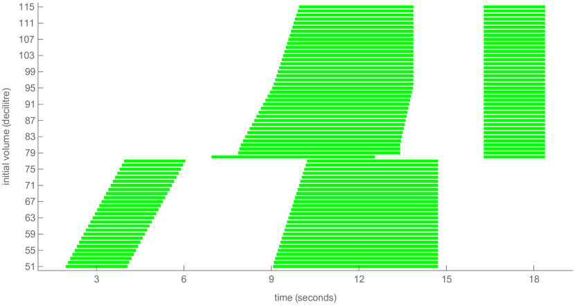
Figure 15: Strategies for the $m$-stable interval $[5.1;8.9]\;$\mathrm{l}$$ (for $U=11.5\;$\mathrm{l}$$)

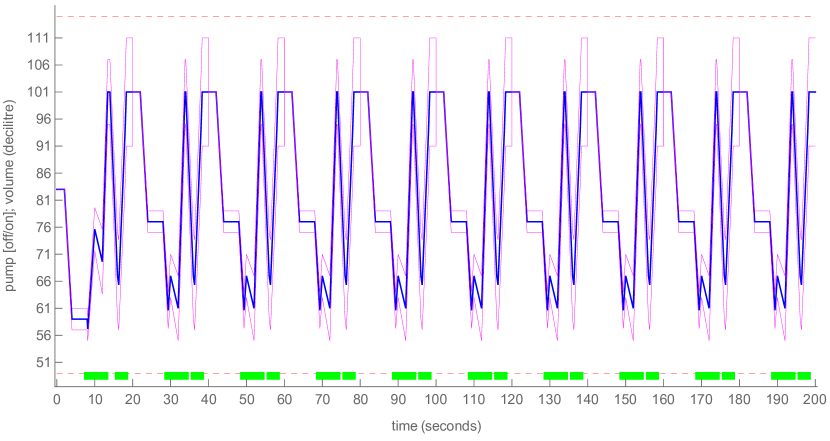
Figure 16: Simulation of 10 cycles

References

- [1] R. Alur, C. Courcoubetis, T. A. Henzinger, and P.-H. Ho. Hybrid automata: An algorithmic approach to the specification and verification of hybrid systems. In R. L. Grossman, A. Nerode, A. P. Ravn, and H. Rischel, editors, Hybrid Systems, pages 209–229, Berlin, Heidelberg, 1993. Springer Berlin Heidelberg.
- [2] R. Alur and D. L. Dill. A theory of timed automata. Theoretical Computer Science, 126(2):183–235, Apr. 1994.
- [3] R. Alur, S. La Torre, and G. J. Pappas. Optimal paths in weighted timed automata. In M. D. Di Benedetto and A. L. Sangiovani-Vincentelli, editors, Proceedings of the 4th International Workshop on Hybrid Systems: Computation and Control (HSCC'01), volume 2034 of Lecture Notes in Computer Science, pages 49–62. Springer-Verlag, Mar. 2001.
- [4] G. Bacci, P. Bouyer, U. Fahrenberg, K. G. Larsen, N. Markey, and P.-A. Reynier. Optimal and Robust Controller Synthesis: Using Energy Timed Automata with Uncertainty, 2018. arXiv:1805.00847 [cs.FL].
- [5] G. Behrmann, A. Cougnard, A. David, E. Fleury, K. G. Larsen, and D. Lime. UPPAAL-Tiga: Time for playing games! In W. Damm and H. Hermanns, editors, Computer Aided Verification, 19th International Conference, CAV 2007, Berlin, Germany, July 3-7, 2007, Proceedings, volume 4590 of Lecture Notes in Computer Science, pages 121–125. Springer, 2007.
- [6] G. Behrmann, A. Fehnker, T. Hune, K. G. Larsen, P. Pettersson, J. Romijn, and F. Vaandrager. Minimum-cost reachability for priced timed automata. In M. D. Di Benedetto and A. L. Sangiovani-Vincentelli, editors, Proceedings of the 4th International Workshop on Hybrid Systems: Computation and Control (HSCC'01), volume 2034 of Lecture Notes in Computer Science, pages 147–161. Springer-Verlag, Mar. 2001.
- [7] A. Bemporad, G. Ferrari-Trecate, and M. Morari. Observability and controllability of piecewise affine and hybrid systems. IEEE Transactions on Automatic Control, 45(10):1864–1876, 2000.
- [8] M. Bisgaard, D. Gerhardt, H. Hermanns, J. Krcál, G. Nies, and M. Stenger. Battery-aware scheduling in low orbit: The GomX-3 case. In J. S. Fitzgerald, C. L. Heitmeyer, S. Gnesi, and A. Philippou, editors, FM 2016: Formal Methods - 21st International Symposium, Limassol, Cyprus, November 9-11, 2016, Proceedings, volume 9995 of Lecture Notes in Computer Science, pages 559–576, 2016.
- [9] V. D. Blondel, O. Bournez, P. Koiran, and J. N. Tsitsiklis. The stability of saturated linear dynamical systems is undecidable. Journal of Computer and System Sciences, 62(3):442–462, 2001.
- [10] V. D. Blondel and J. N. Tsitsiklis. Complexity of stability and controllability of elementary hybrid systems. Automatica, 35(3):479–489, 1999.
- [11] P. Bouyer, U. Fahrenberg, K. G. Larsen, and N. Markey. Timed automata with observers under energy constraints. In K. H. Johansson and W. Yi, editors, Proceedings of the 13th International Workshop on Hybrid Systems: Computation and Control (HSCC'10), pages 61–70. ACM Press, Apr. 2010.
- [12] P. Bouyer, U. Fahrenberg, K. G. Larsen, N. Markey, and J. Srba. Infinite runs in weighted timed automata with energy constraints. In F. Cassez and C. Jard, editors, Proceedings of the 6th International Conferences on Formal Modelling and Analysis of Timed Systems (FORMATS'08), volume 5215 of Lecture Notes in Computer Science, pages 33–47. Springer-Verlag, Sept. 2008.
- [13] P. Bouyer, K. G. Larsen, and N. Markey. Lower-bound constrained runs in weighted timed automata. Performance Evaluation, 73:91–109, Mar. 2014.
- [14] M. Bozga, R. Iosif, and Y. Lakhnech. Flat parametric counter automata. In M. Bugliesi, B. Preneel, V. Sassone, and I. Wegener, editors, Proceedings of the 33rd International Colloquium on Automata, Languages and Programming (ICALP'06)) – Part II, volume 4052 of Lecture Notes in Computer Science, pages 577–588. Springer-Verlag, July 2006.
- [15] F. Cassez, A. David, E. Fleury, K. G. Larsen, and D. Lime. Efficient on-the-fly algorithms for the analysis of timed games. In M. Abadi and L. de Alfaro, editors, CONCUR 2005 - Concurrency Theory, 16th International Conference, CONCUR 2005, San Francisco, CA, USA, August 23-26, 2005, Proceedings, volume 3653 of Lecture Notes in Computer Science, pages 66–80. Springer, 2005.
- [16] F. Cassez, J. J. Jensen, K. G. Larsen, J.-F. Raskin, and P.-A. Reynier. Automatic synthesis of robust and optimal controllers – an industrial case study. In R. Majumdar and P. Tabuada, editors, Proceedings of the 12th International Workshop on Hybrid Systems: Computation and Control (HSCC'09), volume 5469 of Lecture Notes in Computer Science, pages 90–104. Springer-Verlag, Apr. 2009.
- [17] H. Comon and Y. Jurski. Multiple counters automata, safety analysis, and Presburger arithmetic. In A. J. Hu and M. Y. Vardi, editors, Proceedings of the 10th International Conference on Computer Aided Verification (CAV'98), volume 1427 of Lecture Notes in Computer Science, pages 268–279. Springer-Verlag, June-July 1998.
- [18] A. David, P. G. Jensen, K. G. Larsen, A. Legay, D. Lime, M. G. Sørensen, and J. H. Taankvist. On time with minimal expected cost! In F. Cassez and J. Raskin, editors, Automated Technology for Verification and Analysis - 12th International Symposium, ATVA 2014, Sydney, NSW, Australia, November 3-7, 2014, Proceedings, volume 8837 of Lecture Notes in Computer Science, pages 129–145. Springer, 2014.
- [19] A. David, P. G. Jensen, K. G. Larsen, M. Mikucionis, and J. H. Taankvist. Uppaal Stratego. In C. Baier and C. Tinelli, editors, Tools and Algorithms for the Construction and Analysis of Systems - 21st International Conference, TACAS 2015, Held as Part of the European Joint Conferences on Theory and Practice of Software, ETAPS 2015, London, UK, April 11-18, 2015. Proceedings, volume 9035 of Lecture Notes in Computer Science, pages 206–211. Springer, 2015.
- [20] G. Frehse. Phaver: algorithmic verification of hybrid systems past hytech. STTT, 10(3):263–279, 2008.
- [21] S. Jha, S. A. Seshia, and A. Tiwari. Synthesis of optimal switching logic for hybrid systems. In S. Chakraborty, A. Jerraya, S. K. Baruah, and S. Fischmeister, editors, Proceedings of the 11th International Conference on Embedded Software, EMSOFT 2011, part of the Seventh Embedded Systems Week, ESWeek 2011, Taipei, Taiwan, October 9-14, 2011, pages 107–116. ACM, 2011.
- [22] N. Markey. Verification of Embedded Systems – Algorithms and Complexity. Mémoire d'habilitation, École Normale Supérieure de Cachan, France, Apr. 2011.
- [23] S. Miremadi, Z. Fei, K. Åkesson, and B. Lennartson. Symbolic supervisory control of timed discrete event systems. IEEE Trans. Contr. Sys. Techn., 23(2):584–597, 2015.
- [24] D. Monniaux. Quantifier elimination by lazy model enumeration. In T. Touili, B. Cook, and P. B. Jackson, editors, Computer Aided Verification, 22nd International Conference, CAV 2010, Edinburgh, UK, July 15-19, 2010. Proceedings, volume 6174 of Lecture Notes in Computer Science, pages 585–599. Springer, 2010.
- [25] A. Phan, M. R. Hansen, and J. Madsen. EHRA: Specification and analysis of energy-harvesting wireless sensor networks. In S. Iida, J. Meseguer, and K. Ogata, editors, Specification, Algebra, and Software - Essays Dedicated to Kokichi Futatsugi, volume 8373 of Lecture Notes in Computer Science, pages 520–540. Springer, 2014.
- [26] Quasimodo. Quantitative system properties in model-driven design of embedded systems. http://www.quasimodo.aau.dk/.
- [27] G. von Bochmann, M. Hilscher, S. Linker, and E. Olderog. Synthesizing and verifying controllers for multi-lane traffic maneuvers. Formal Asp. Comput., 29(4):583–600, 2017.
- [28] Wolfram Research, Inc. Mathematica, Version 11.2. Champaign, IL, 2017.
- [29] H. Zhao, N. Zhan, D. Kapur, and K. G. Larsen. A ``hybrid'' approach for synthesizing optimal controllers of hybrid systems: A case study of the oil pump industrial example. In D. Giannakopoulou and D. Méry, editors, FM 2012: Formal Methods - 18th International Symposium, Paris, France, August 27-31, 2012. Proceedings, volume 7436 of Lecture Notes in Computer Science, pages 471–485. Springer, 2012.