Topological invariants for the Haldane phase of interacting SSH chains – a functional RG approach

Abstract

We present a functional renormalization group approach to interacting topological Green function invariants with a focus on the nature of transitions. The method is applied to chiral symmetric fermion chains in the Mott limit that can be driven into a Haldane phase. We explicitly show that the transition to this phase is accompanied by a zero of the fermion Green function. Our results for the phase boundary are quantitatively benchmarked against DMRG data.

I Introduction

The complete topological classification of non-interacting fermionic insulators and superconductors was a milestone achievement in condensed matter theory Kitaev (2009); Ryu et al. (2010); Qi and Zhang (2010); Hasan and Kane (2010). The result is conveniently summarized in the ten-fold way table which lists the equivalence classes of Hamiltonians depending on spatial dimension and the presence of time-reversal, particle-hole and chiral symmetries. In terms of Bloch Hamiltonians $\mathcal{H}(\mathbf{k})$, this amounts to investigating the topological properties of the map $\mathbf{k}\rightarrow\mathcal{H}(\mathbf{k})$. Two $\mathcal{H}(\mathbf{k})$ are equivalent if they can be deformed into each other without breaking the specified symmetries or closing the gap.

Soon after, efforts were directed to a generalization for interacting systems, leading to the concept of symmetry protected topological states (SPT) Pollmann et al. (2010); Fidkowski and Kitaev (2010, 2011); Turner and Vishwanath (2013); Wen (2017). The (non-degenerate) ground states of two many-body Hamiltonians are equivalent if they can be adiabatically connected without breaking the defining symmetries (which is possible if and only if the Hamiltonians can be deformed into each other without closing of the many-body gap). To date, the topological classification for fermionic interacting system is not known completely, except in one spatial dimension.

Given a certain microscopic model, one would like to know its ground state’s equivalence class, usually as a function of the model parameter. This is achieved in terms of topological invariants, which can be formulated in various equivalent ways. In the noninteracting case, the invariant can be based on the eigenstates of Bloch Hamiltonians $\mathcal{H}(\mathbf{k})$. Given a control parameter in $\mathcal{H}$, it can be shown that the (integer valued) topological invariant $\nu\left(\mathcal{H}\right)$ can only change at gapless points where $\mathcal{H}(\mathbf{k})$ has zero eigenvalues at some momentum $\mathbf{k}$ in the Brillouin zone: If two Bloch Hamiltonians feature different (the same) invariants, they cannot (can always) be deformed into each other without closing the gap.

In the interacting case, one can still consider the noninteracting expressions for the invariants if one replaces the Bloch Hamiltonian with the inverse single-particle retarded $T=0$ Green function at vanishing frequency, $\mathcal{H}(\mathbf{k})\rightarrow-G^{-1}(i\omega=0,\mathbf{k})$ Volovik (2003). In the mathematical formulation of $\nu\left(G\right)$ to be detailed below, $G$ and $G^{-1}$ are used on equal footing and correspondingly, $\nu$ can change at poles of $G$, where $G^{-1}=0$ for some momentum in the Brillouin zone, or at zeros with $G=0$ Gurarie (2011). A pole is interpreted as a closing of the single-particle excitation gap whereas a zero indicates a breakdown of the single-particle picture and is ruled out in the noninteracting case (for bounded Hamiltonians). As shown in Ref. Manmana et al. (2012), a zero can be both compatible with a many-body gap closing (e.g., the spin gap closes while the charge gap stays open) or with a unique, gapped ground state (no gap closing). It is therefore possible that two different noninteracting topological phases can be adiabatically deformed into each other when interactions are switched on but that the noninteracting invariant still changes, for a recent experimental proposal see Ref. Yoshida et al. (2018). Thus, a new classification becomes necessary in interacting systems. This is also reflected in the recently proposed many-body invariants of Refs. Shapourian et al. (2016); Shiozaki et al. (2017).

Figure 1: Model Hamiltonians used in this paper. The sublattices are denoted by A and B, straight lines denote single-particle hopping $t\pm\delta t$ and curved arrows denote Hubbard interactions $U$. Spin-Spin interactions $J$ are denoted by straight arrows.

In the following, we focus on the evaluation of the Green function invariant $\nu\left(G\right)$ with an emphasis on the nature of the transition points. Considerable effort has been directed to one-dimensional systems. In many cases of interest, the Green function can be calculated analytically. For example, You et al. used an unconventional perturbation theory in the non-interacting part of the Hamiltonian to demonstrate that when a topological phase transition between two noninteracting phases is gapped by interactions, the poles will be replaced by Green function zeros You et al. (2014). Moreover, in Ref. Manmana et al. (2012), Green functions at transition points were calculated analytically for several models at special points in parameter space. In the general case, however, a numerical evaluation of the Green function is required. Previous studies Manmana et al. (2012); Yoshida et al. (2014) employed the density matrix renormalization group (DMRG) White (1992) to compute the Green function winding number. Although the DMRG and its underlying matrix-product state formulation is very well suited to determine one-dimensional topological phases via entanglement properties Pollmann et al. (2010), it has severe shortcomings when it comes to calculating Green function winding numbers: In order to compute $\nu(G)$, the Green function is required at zero frequency $G(i\omega=0,\mathbf{k})$ in the thermodynamic limit, which is generally difficult for the DMRG Schollwöck (2005, 2011). One can, e.g., use a real-time algorithm to generate Green functions via a Fourier transform; the accessible timescales, however, are limited by the entanglement growth, and instead of $i\omega=0$, one can determine $G$ reliably only at finite frequencies. Since the invariant is quantized, this should not affect the results, except in the vicinity of points in parameter space where $\nu$ changes. However, as we discussed above, a precise assessment of the type of singularity occurring at these points (Green function zero or pole) is essential.

In this paper, we propose the fermionic functional renormalization group (fRG) Kopietz et al. (2010); Metzner et al. (2012) as an alternative method to numerically evaluate Green function invariants. We show that the fRG, set up in a Matsubara formulation and momentum space, is capable of evaluating Green functions at $i\omega=0$ and easily tells poles from zeros. We put an emphasis on transition points and show in detail how the zeros of $G$ are understood in the framework of the self-energy Honerkamp and Salmhofer (2003). Although bulk-boundary correspondence is often discussed in the context of topological systems, in the following we limit ourselves to the bulk perspective (though fRG can also be applied to finite systems). While the fRG can be set up in arbitrary dimension, for a concrete example, we focus on one-dimensional systems with both charge conservation and many-body chiral symmetry, i.e., interacting variants of the Su-Schrieffer-Heeger (SSH) chain Su et al. (1979). In this case, $\nu\left(G\right)$ takes the form of a winding number and the classification is $\mathbb{Z}$ for noninteracting and $\mathbb{Z}_{4}$ for interacting systems Fidkowski and Kitaev (2010, 2011); Turner et al. (2011). A common criticism of the fRG method is its perturbative character. Although the Green functions calculated within our fRG truncation scheme below are guaranteed to be correct to second order in the interaction only, the fRG results contain partial resummation of diagrams to infinite order. For our models, we show that we can capture Mott physics both qualitatively and quantitatively with reasonable accuracy.

The rest of the paper is structured as follows. In Sec. II we present the model Hamiltonian and discuss its topological phase diagram qualitatively. In Sec. III we define the appropriate Green function winding number and show how it is computed from the self-energy found by fRG. In Sec. IV we explain the fRG approach. The numerical results are presented in Sec. V along with a comparison to DMRG and we conclude in Sec. VI.

II Model Hamiltonian

We start by defining the Hamiltonian $H$ that we will employ in the following (see Fig. 1 for a sketch), closely following Refs. Manmana et al. (2012); Yoshida et al. (2014):

$$H_{\mathrm{SSH}} \!= \!-\!\!\sum_{j}[\left(t\!-\!\delta t\right)\!c_{j,A}^{\dagger}c_{j,B}$$

$$\!+\!\left(t\!+\!\delta t\right)\!c_{j,B}^{\dagger}c_{j+1,A}\!+\!h.c.]$$

$$H \!= \!H_{\mathrm{SSH},\uparrow}\!+H_{\mathrm{SSH},\downarrow}$$

$$+ U\!\!\sum_{j;s=A,B}\!\left(n_{j,s,\uparrow}\!-\!\frac{1}{2}\right)\!\left(n_{j,s,\downarrow}\!-\!\frac{1}{2}\right)$$

$$+ J\sum_{j}\mathbf{S}_{j,A}\cdot\mathbf{S}_{j,B}.$$

We denote fermion creators/annihilators on site $j$ of an infinite one-dimensional lattice by $c_{j,s}^{(\dagger)}$, with each unit cell split into sublattices $s=\{A,B\}$. The lattice constant is set to unity and we work at half-filling throughout. The Hamiltonian $H_{\mathrm{SSH}}$ is the SSH model which features a single spinless fermion per lattice site and hoppings alternating between $t+\delta t$ and $t-\delta t$. We then generalize to spinful fermions $c_{j,s,\sigma}^{(\dagger)}$ in $H$ and introduce on-site Hubbard interactions $U$ as well as an intra-unit cell spin-spin exchange interaction $J$. Here, $\mathbf{S}=(S^{x},S^{y},S^{z})^{\mathrm{T}}$ denotes the spin operator where $S^{i}=\frac{1}{2}\sum_{\sigma,\sigma^{\prime}}c_{\sigma}^{\text{$\dagger$}}\sigma_{\sigma\sigma^{\prime}}^{i}c_{\sigma^{\prime}}$ for $i=x,y,z$ (site/sublattice indices suppressed).

The model Hamiltonians $H_{\mathrm{SSH}}$ and $H$ are invariant under time-reversal, particle-hole, and chiral symmetry; the single-particle version of $H_{\mathrm{SSH}}$ falls into the class BDI of the noninteracting Altland-Zirnbauer classification Altland and Zirnbauer (1997). The formulation of the topological invariant rests on chiral symmetry, it takes the form Gurarie (2011)

$$H=U_{C}^{\dagger}H^{\star}U_{C},$$ (3)

where the star denotes complex conjugation not affecting fermionic operators. The action of $U_{C}$ on fermion creation and anihilation operators is defined as

$$U_{C}^{\dagger}c_{\alpha}U_{C} =\sum_{\beta}c_{\beta}^{\dagger}\left[\tau_{z}\right]_{\beta\alpha},$$ (4)

$$U_{C}^{\dagger}c_{\alpha}^{\dagger}U_{C} =\sum_{\beta}\left[\tau_{z}\right]_{\alpha\beta}c_{\beta},$$ (5)

where $\alpha,\beta$ contain the single-particle indices as appropriate for the different models discussed above and $\tau_{z}$ is the third Pauli matrix in sublattice space. Note that the site- and spin-labels (if present) are not modified. Before we investigate the restrictions on the single-particle ground state Green function arising from chiral symmetry and formulate the winding number, we qualitatively discuss the physics of $H_{\mathrm{SSH}}$ and $H$, following Ref. Manmana et al. (2012).

The SSH chain $H_{\mathrm{SSH}}$ is gapped for $\delta t\neq 0$. For the special point $\delta t=t$, there is no hopping between A and B sublattice sites of the same unit cell while there is dimerization between B and A sublattice site across the unit cell. If we would terminate the chain at an A site, we would have a single-particle edge state, thus $\delta t>0$ corresponds to the topological, $\delta t<0$ to the trivial phase. At the transition point $\delta t=0$, the Green function has a pole. Now consider $H$ with $J=0$, i.e., a spinful SSH chain featuring a Hubbard interaction $U>0$. At $\delta t=0$, the system is a Mott insulator at half filling with low energy spin-1/2 degrees of freedom coupled anti-ferromagnetically with strength $\sim t^{2}/U>0$ Lieb and Wu (1968); Manmana et al. (2012); Barbiero et al. (2018). This half-integer spin chain has a charge gap but gapless spin excitations. For $\delta t\neq 0$, these spin couplings alternate in strength, the spins pair up, form singlets, and we obtain a spin gap. In conclusion, the addition of the Hubbard term $U>0$ does not modify the topological phase diagram from the case $U=0$; however, the transition in $\nu(G)$ at $\delta t=0$ is now accompanied by a zero of the Green function reflective of the collective nature of the gapless spin excitation when expressed in terms of fermion operators. Since the non-interacting Hamiltonian $H_{\mathrm{SSH}}$ vanishes for $\delta t=0$ and $k=\pi$, the appearance of a Green function zero can also be derived using perturbation theory as in Ref. You et al. (2014).

We now consider $\delta t<0$ (which gaps $H_{\mathrm{SSH}}$) and switch on a finite spin-spin exchange interaction $J$ in $H$, which we choose to be negative (ferromagnetic). For $|J|\gg t^{2}/U$, it leads to the formation of effective spin-1 objects in each unit cell which are coupled anti-ferromagnetically. This state is known to be in the Haldane phaseManmana et al. (2012), which is gapped and topological with spin-1/2 edge excitations, again hinting towards a closing of a spin gap and corresponding Green function zero at the transition point. In the following, we keep $J<0$ constant but increase $U$ to tune the transition from a trivial phase at $|J|\ll t^{2}/U$ to the Haldane phase for $|J|\gg t^{2}/U$. It is the central goal of this paper to show that the fermionic fRG is capable of detecting the Haldane phase via the Green function winding number and unambiguously identifies the zero at the transition. We note that in Ref. Anfuso and Rosch (2007) it was demonstrated that the Haldane phase built from spin-1/2 fermions can be adiabatically connected to a trivial phase even without gap closing, but this required the breaking of chiral symmetry.

III Green function winding number

We start the discussion of topological invariants from the non-interacting SSH model $H_{\mathrm{SSH}}$, Eq. (II). After a spatial Fourier-transform, $c_{j,s}=\int_{-\pi}^{\pi}\frac{dk}{2\pi}c_{k,s}e^{ikj}$, we obtain

$$H_{\mathrm{SSH}}=\int_{-\pi}^{\pi}\frac{dk}{2\pi}\,c_{k}^{\dagger}\mathcal{H}_{\mathrm{SSH}}(k)c_{k},$$ (6)

where $c_{k}=(c_{k,A},\,c_{k,B})^{\mathrm{T}}$. The corresponding Bloch Hamiltonian reads

$$\mathcal{H}_{\mathrm{SSH}}(k)=\left(\begin{array}[]{cc}0&h_{\mathrm{SSH}}(k)\\ h_{\mathrm{SSH}}^{\dagger}(k)&0\end{array}\right),$$ (7)

with $h_{\mathrm{SSH}}(k)=-\left(t+\delta t\right)e^{-ik}-\left(t-\delta t\right)$. Topological invariants for non-interacting insulators with chiral symmetry in odd dimensions are winding numbers of $\mathbb{Z}$-type. In one dimension, the invariant can be expressed as Volovik (2003)

$$\nu_{\mathrm{SSH}} =\int_{-\pi}^{\pi}\frac{dk}{4\pi i}\,\mathrm{tr}\left[\tau_{z}\mathcal{H}_{\mathrm{SSH}}^{-1}(k)\partial_{k}\mathcal{H}_{\mathrm{SSH}}(k)\right]$$ (8)

$$=\int_{-\pi}^{\pi}\frac{dk}{2\pi i}\,\partial_{k}\mathrm{log}\,h_{\mathrm{SSH}}^{\dagger}(k),$$

counting how often $h_{\mathrm{SSH}}(k)$ winds around the origin of the complex plan, $\nu_{\mathrm{SSH}}\in\mathbb{Z}$. The winding is trivial (zero) for $\delta t<0$ and nontrivial for $\delta t>0$. The off-diagonal form of Eq. (7), and thus the existence of the winding number $\nu_{\mathrm{SSH}}$, is a consequence of the chiral symmetry, Eq. (3), which enforces

$$\mathcal{H}_{\mathrm{SSH}}(k)=-\tau_{z}\mathcal{H}_{\mathrm{SSH}}\left(k\right)\tau_{z}.$$ (9)

We now generalize the definition of the winding number to arbitrary chiral, translational invariant and possibly interacting systems featuring a a gap of single-particle excitations. The central object of the following discussion is the imaginary frequency Green function (at zero temperature). It is defined as a Fourier transform of the imaginary time Green function,

$$G(i\omega)=\int_{0}^{\infty}d\tau\,e^{i\omega\tau}G(\tau),\leavevmode\nobreak\ G_{\alpha\beta}(\tau)=-\left\langle T_{\tau}c_{\alpha}\left(\tau\right)c_{\beta}^{\dagger}\right\rangle,$$ (10)

where $c_{\alpha}\left(\tau\right)=e^{H\tau}c_{\alpha}\,e^{-H\tau}$, $T_{\tau}$ denotes time-ordering, and $\alpha,\beta$ are single-particle multiindices $\alpha,\beta$. After a spatial Fourier transform the Green function $G(i\omega,k)$ is diagonal in the crystal momentum $k$. It can be shown Gurarie (2011) that under a general chiral symmetry (which can always be represented by $\tau_{z}$ in some basis), $G$ transforms as

$$G^{-1}(i\omega,k)=-\tau_{z}G^{-1}\left(-i\omega,k\right)\tau_{z}.$$ (11)

Analogous statements are true for other symmetries Gurarie (2011). Based on Eq. (11), winding numbers were defined, first using integration both over $\omega$ and $k$ Volovik (2003); Gurarie (2011). However, it was shown in Ref. Wang and Zhang, 2012 that, given a non-singular $G(i\omega,k)$, all topological information is contained in the Green function at $i\omega=0$, which is a well-defined limit for a gapped system. In this case, Eq. (11) implies the form

$$-G^{-1}(i\omega=0,k)=\left(\begin{array}[]{cc}0&h\left(k\right)\\ h^{\dagger}\left(k\right)&0\end{array}\right),$$ (12)

with the depicted matrix structure in sublattice space and $h\left(k\right)$ a matrix in the remaining degrees of freedom. The Green function winding number then reads Manmana et al. (2012)

$$\nu =\int_{-\pi}^{\pi}\frac{dk}{4\pi i}\,\mathrm{tr}\left[\tau_{z}G(0,k)\partial_{k}G^{-1}(0,k)\right]$$ (13)

$$=\int_{-\pi}^{\pi}\frac{dk}{2\pi i}\,\mathrm{tr}\left[\partial_{k}\mathrm{log}\,h^{\dagger}(k)\right],$$

counting the complex plane winding of the eigenvalues of $h(k)$ around the origin. Mathematically, the robustness of $\nu$ can be formulated as follows: Assume that the system [and $h(k)$] depends on some external parameter $\xi$, then the winding number is invariant under small changes of $\xi$, as one can see from $\partial_{\xi}\nu=0$ Manmana et al. (2012). For noninteracting systems with Bloch Hamiltonian $\mathcal{H}(k)$, from the relation $G(i\omega,k)=1/\left[i\omega-\mathcal{H}(k)\right]$, we have $\,-G^{-1}(i\omega=0,k)=\mathcal{H}(k)$ so that Eq. (13) specializes to Eq. (8) with $h\rightarrow h_{\mathrm{SSH},\uparrow}+h_{\mathrm{SSH},\downarrow}$.

Based on Eq. (13), it is evident that besides poles [vanishing eigenvalues of $G^{-1}(0,k)$] also zeros [vanishing eigenvalues of $G(0,k)$] can cause a change of the winding number $\nu$ Gurarie (2011). Poles are familiar from the non-interacting case and indicate a zero-energy single-particle excitation. The presence of zeros indicates a complete loss of single particle coherence and is an inherent many-body phenomenon. By passing through zeros, the winding number can change without a gap closing. This is the mechanism that causes the collapse of free classification of topological fermion phases in the presence of interactions. Alternatively, the zero can occur along with a many-body gap closing; in this case, it signals a topological phase transition.

Given a generic interacting fermion system, it is thus desirable to devise a numerical method to (i) compute the winding number $\nu$ (or Chern-number, as appropriate) in the case that $G(0,k)$ is non-singular, and (ii) classify the nature of the points in parameter space where $\nu$ changes, i.e., tell poles from zeros. It is our goal to show how the fRG can be used for both purposes.

The central object obtained from the fRG is the single-particle self-energy $\Sigma(i\omega,k)$. The Green function is then given by

$$G\left(i\omega,k\right)=\frac{1}{i\omega-\mathcal{H}_{0}(k)-\Sigma\left(i\omega,k\right)},$$ (14)

where $\mathcal{H}_{0}(k)$ is the non-interacting Bloch Hamiltonian. The presence of a zero is tied to a vanishing quasiparticle weight for some $k$ in the Brillouin zone Honerkamp and Salmhofer (2003); Bruus and Flensberg (2004),

$$Z(k)\equiv\left(1-\partial_{\omega}\mathrm{Im}\Sigma(i\omega,k)|_{\omega=0}\right)^{-1}.$$ (15)

This becomes apparent if one rewrites

$$G\left(i\omega\simeq 0,k\right)=\frac{Z(k)}{i\omega-\mathcal{H}_{\mathrm{top}}(k)},$$ (16)

with

$$\mathcal{H}_{\mathrm{top}}(k) =Z(k)\left[\mathcal{H}_{0}(k)+\Sigma\left(i\omega=0,k\right)\right].$$ (17)

If $Z(k)$ is finite, the Green function winding number can be obtained from $\mathcal{H}_{\mathrm{top}}(k)$, which is off-diagonal as in Eq. (12). A vanishing eigenvalue of $\mathcal{H}_{\mathrm{top}}(k)$ at finite $Z(k)$ indicates the presence of a Green function pole.

IV Functional RG

The functional renormalization group method is an implementation of the RG idea on the basis of many-body vertex functions, see Refs. Kopietz et al. (2010); Metzner et al. (2012) for general introductions. The idea amounts to using an infrared cutoff $\Lambda$ in the bare Matsubara Green function $G_{0}\left(i\omega,k\right)=\left(i\omega-\mathcal{H}_{0}(k)\right)^{-1}$, here we choose a frequency cutoff $G_{0}^{\Lambda}\left(i\omega,k\right)=\Theta\left(|\omega|-\Lambda\right)G_{0}\left(i\omega,k\right).$ Then, the $\Lambda$-dependence carries over to all vertex functions, the simplest of which is the self energy $\Sigma^{\Lambda}\left(i\omega,k\right)$ appearing in the full Green function, see Eq. (14). In the limit $\Lambda=\infty$, the dynamics of the system is frozen and the vertex functions are trivial. The fRG flow equations are an infinite set of coupled differential equations that describe the change of the vertex functions with $\Lambda$. The solution of these flow equations at $\Lambda=0$ (where the cutoff vanishes) yields exact vertex functions of the physical problem. In practice, truncation of the infinite hierarchy of flow equations is required and the resulting vertex functions approximate the exact ones with an agreement of at least order $O(v^{n})$ where $v$ is a proxy for the interaction strength in the Hamiltonian (i.e., $U$ or $J$ in Eq. (II)), and $n=1,2,3,...$ depending on the level of the truncation. Note that unlike perturbation theory, the fRG contains an infinite re-summation of Feynman diagrams. We have recently developed a $k$-space fRG approach which is correct to order $O(v^{2})$ for one-dimensional, translationally invariant fermion systems in equilibrium, see Ref. Sbierski and Karrasch, 2017. There, we have applied the fRG to a Luttinger liquid with good agreement to alternative exact methods. We refer the reader to Ref. Sbierski and Karrasch, 2017 for further discussion of the method.

For the self-energy, the flow equation reads Sbierski and Karrasch (2017)

$$\partial_{\Lambda}\Sigma_{\alpha^{\prime}\alpha}^{\Lambda}\left(i\omega,k\right) \!= \!-\!\int_{-\pi}^{\pi}\!\frac{d\bar{k}}{2\pi}\!\int_{-\infty}^{+\infty}\!\frac{d\bar{\omega}}{2\pi}\sum_{\beta,\beta^{\prime}}S_{\beta\beta^{\prime}}^{\Lambda}\left(i\bar{\omega},\bar{k}\right)$$ (19)

$$\times V_{\beta^{\prime}\alpha^{\prime};\beta\alpha}^{\Lambda}\left(\begin{array}[]{ccc}i\bar{\omega},\bar{k};&i\omega,k;&i\bar{\omega},\bar{k}\end{array}\right),$$

where $S^{\Lambda}\left(i\omega,k\right)$ is the single-scale propagator, $S^{\Lambda}=G^{\Lambda}\left(\partial_{\Lambda}\left[G_{0}^{\Lambda}\right]^{-1}\right)G^{\Lambda}$, and $V^{\Lambda}$ the 2-particle vertex where frequency and momentum conservation has been used to eliminate the fourth argument. Initially, $V^{\Lambda}$ is frequency independent, $V^{\Lambda=\infty}\sim U+J$. In a first-order trunctation ($n=1$), the flow of $V^{\Lambda}$ (which is itself of order $v$) would be neglected by setting $V^{\Lambda}\rightarrow V^{\Lambda=\infty}$ in Eq. (19). Evidently, $\Sigma^{\Lambda}\left(i\omega,k\right)$ then turns out to be frequency independent, and consequently $Z(k)=1$ as is apparent from Eq. (15). Thus, the truncation to order $n=2$ with a flowing and frequency-dependent 2-particle vertex $V^{\Lambda}$ is mandatory for our purpose. The full flow equations, including a static but fully momentum dependent feedback for $V^{\Lambda}$ are lengthy and are given in Eqs. (34)-(36) of Ref. Sbierski and Karrasch, 2017.

V Results

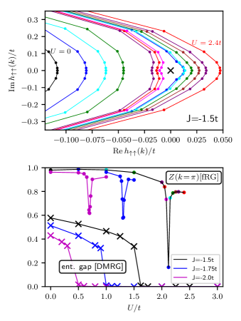
Figure 2: Top panel: fRG results for the Green function winding of the chiral fermion chain $H$ for fixed $\delta t=-t/4$, $J=-1.5t$ with increasing $U$, driving the transition from a trivial to the Haldane phase at $U_{c,\mathrm{fRG}}\simeq 2.1t$. The finite value of $|h_{\uparrow\uparrow}(k)|$ for all $k$ and $U$ reveals the presence of a gap of single-particle excitations across the transition. Bottom panel: The vanishing of the quasiparticle weight $Z(k\!=\!\pi)$ (colored points on black line) confirms the presence of a Green function zero at the transition. The comparison with the more precise DMRG result $U_{c,\mathrm{DMRG}}\simeq 1.6$ based on the entanglement gap indicates a slight overestimation of $U_{c}$ by the fRG. Qualitatively similar results hold for $J=-1.75$ (blue symbols) and $J=-2$ (magenta symbols) for which $U_{c}$ decreases.

We now proceed to present the fRG results for the winding number and the quasiparticle weight for the chiral fermion chain $H$ in Eq. (II). Except at the critical point mentioned at the following, the Green function $G(i\omega,k)$ is found to be regular for all $i\omega$ and $k$ and thus the simplified expression (13) can be applied. As a phase diagram (based on the DMRG entanglement spectrum) can be found in the appendix of Ref. Yoshida et al. (2014), we focus on a single line in parameter space. We let $\delta t=-t/4$, $J=-1.5t$ and increase the Hubbard interaction $U$ to drive the transition from a trivial to a Haldane insulator once $|J|\gg t^{2}/U$. Note that the non-interacting part of $H$ is gapped and convergence issues of the fRG as encountered for $\delta t=0$ in Ref. Sbierski and Karrasch, 2017 are absent. Due to $S_{z}$ conservation and rotation symmetry, the off-diagonal blocks of $-G^{-1}(i\omega=0,k)$ are of the form

$$h(k)=\left(\begin{array}[]{cc}h_{\uparrow\uparrow}(k)&0\\ 0&h_{\downarrow\downarrow}(k)\end{array}\right)$$ (20)

with $h_{\uparrow\uparrow}=h_{\downarrow\downarrow}$. In Fig. 2, the top panel depicts the complex value of $h_{\uparrow\uparrow}(k)$ for increasing $U$ in the vicinity of $k=\pi$ (identified by $\mathrm{Im}\left[h_{\uparrow\uparrow}(k=\pi)\right]=0$). The origin of the complex plane is denoted by a black cross. The phase winding of $h_{\uparrow\uparrow}(k)$ is trivial (leading to $\nu=0$) for $U<U_{c,\mathrm{fRG}}$ and non-trivial (winding once around the origin, $|\nu|=2$ due to spin) for $U>U_{c,\mathrm{fRG}}$ with $U_{c,\mathrm{fRG}}\simeq 2.1t$. For all $U$ and $k$, the magnitude of $|h_{\uparrow\uparrow}|$ is larger than a constant, signaling the presence of gapped single-particle excitations (no pole) throughout the transition.

The lower panel depicts the behavior of $Z(k\!=\!\pi)$ (thin black line) which sharply drops in the vicinity of the transition and confirms the presence of a Green function zero at the transition. The lowest value found is below 0.2 for $U=2.12t$. To gauge the quantitative reliability of the fRG results, we have calculated the phase boundary using the entanglement gap from DMRG [imaginary time evolution with a bond dimension of $\chi=320$, see Refs. Schollwöck, 2011 and Karrasch and Kennes, 2016]. The data is shown as black crosses and signals the transition at a critical value of $U_{c,\mathrm{DMRG}}\simeq 1.6$, slightly smaller than the fRG value. Qualitatively similar results hold for different values of $J$, see blue and magenta symbols for $J=-1.75$ and $J=-2$, respectively.

VI Conclusion

We presented the fermionic fRG method as a valuable tool to study SPT phases in terms of Green function winding numbers. Our emphasis was on the nature of the transition between different phases. We explicitly showed for a topological Mott insulator chain how zeros of the Green function can be unambiguously identified from the self-energy. Although the phase diagram itself can be determined using more accurate methods such as the DMRG, obtaining the Green function in the limit $i\omega\rightarrow 0$ is a difficult task, and the fRG offers complementary, qualitative information. It would be interesting to apply the fRG to higher dimensional SPTs where accurate reference methods are sparse and the nature of the transition is less obvious. We remark that similar applications have been put forward in the “Hierachy of correlations” approach of Ref. Gómez-León, 2016.

References

- Kitaev (2009) A. Kitaev, in AIP Conf. Proc. 1134 (2009).
- Ryu et al. (2010) S. Ryu, A. P. Schnyder, A. Furusaki, and A. W. W. Ludwig, New J. Phys. 12, 065010 (2010).
- Qi and Zhang (2010) X.-L. Qi and S.-C. Zhang, Rev. Mod. Phys. 83, 1057 (2010).
- Hasan and Kane (2010) M. Z. Hasan and C. L. Kane, Rev. Mod. Phys. 82, 3045 (2010).
- Pollmann et al. (2010) F. Pollmann, A. M. Turner, E. Berg, and M. Oshikawa, Phys. Rev. B 81, 064439 (2010).
- Fidkowski and Kitaev (2010) L. Fidkowski and A. Kitaev, Phys. Rev. B 81, 134509 (2010).
- Fidkowski and Kitaev (2011) L. Fidkowski and A. Kitaev, Phys. Rev. B 83, 075103 (2011).
- Turner and Vishwanath (2013) A. Turner and A. Vishwanath, arXiv 1301.0330 (2013).
- Wen (2017) X. G. Wen, Rev. Mod. Phys. 89 (2017).
- Volovik (2003) G. Volovik, The universe in a helium droplet (Oxford University Press, Oxford, 2003).
- Gurarie (2011) V. Gurarie, Phys. Rev. B 83, 085426 (2011).
- Manmana et al. (2012) S. R. Manmana, A. M. Essin, R. M. Noack, and V. Gurarie, Phys. Rev. B 86, 205119 (2012).
- Yoshida et al. (2018) T. Yoshida, I. Danshita, R. Peters, and N. Kawakami, Phys. Rev. Lett. 121, 025301 (2018).
- Shapourian et al. (2016) H. Shapourian, K. Shiozaki, and S. Ryu, Phys. Rev. Lett. 118, 216402 (2016).
- Shiozaki et al. (2017) K. Shiozaki, H. Shapourian, K. Gomi, and S. Ryu, (2017), arXiv:1710.01886 .
- You et al. (2014) Y. Z. You, Z. Wang, J. Oon, and C. Xu, Phys. Rev. B 90, 060502 (2014).
- Yoshida et al. (2014) T. Yoshida, R. Peters, S. Fujimoto, and N. Kawakami, Phys. Rev. Lett. 112, 196404 (2014).
- White (1992) S. R. White, Phys. Rev. Lett. 69, 2863 (1992).
- Schollwöck (2005) U. Schollwöck, Rev. Mod. Phys. 77, 259 (2005).
- Schollwöck (2011) U. Schollwöck, Annals of Physics 326, 96 (2011).
- Kopietz et al. (2010) P. Kopietz, L. Bartosch, and F. Schütz, Introduction to the Functional Renormalization Group (Springer, 2010).
- Metzner et al. (2012) W. Metzner, M. Salmhofer, C. Honerkamp, V. Meden, and K. Schönhammer, Rev. Mod. Phys. 84, 299 (2012).
- Honerkamp and Salmhofer (2003) C. Honerkamp and M. Salmhofer, Phys. Rev. B 67, 174504 (2003).
- Su et al. (1979) W. P. Su, J. R. Schrieffer, and A. J. Heeger, Phys. Rev. Lett. 42, 1698 (1979).
- Turner et al. (2011) A. M. Turner, F. Pollmann, and E. Berg, Phys. Rev. B 83, 075102 (2011).
- Altland and Zirnbauer (1997) A. Altland and M. R. Zirnbauer, Phys. Rev. B 55, 1142 (1997).
- Lieb and Wu (1968) E. H. Lieb and F. Y. Wu, Phys. Rev. Lett. 20, 1445 (1968).
- Barbiero et al. (2018) L. Barbiero, L. Santos, and N. Goldman, arXiv 1803.06957 (2018).
- Anfuso and Rosch (2007) F. Anfuso and A. Rosch, Phys. Rev. B 75, 144420 (2007).
- Wang and Zhang (2012) Z. Wang and S.-C. Zhang, Phys. Rev. X 2, 031008 (2012).
- Bruus and Flensberg (2004) H. Bruus and K. Flensberg, Many-Body Quantum Theory in Condensed Matter Physics (Oxford Graduate Texts, 2004).
- Sbierski and Karrasch (2017) B. Sbierski and C. Karrasch, Phys. Rev. B 96, 235122 (2017).
- Karrasch and Kennes (2016) C. Karrasch and D. M. Kennes, Comp. Phys. Comm. 200, 37 (2016).
- Gómez-León (2016) Á. Gómez-León, Phys. Rev. B 94, 035144 (2016).