The CARMENES search for exoplanets around M dwarfs:
A low-mass planet in the temperate zone of the nearby K2-18

Abstract

K2-18 is a nearby M2.5 dwarf, located at 34 pc and hosting a transiting planet which was first discovered by the K2 mission and later confirmed with Spitzer Space Telescope observations. With a radius of $\sim 2\,R_{\oplus}$ and an orbital period of $\sim 33$ days, the planet lies in the temperate zone of its host star and receives stellar irradiation similar to Earth. Here we perform radial velocity follow-up observations with the visual channel of CARMENES with the goal of determining the mass and density of the planet. We measure a planetary semi-amplitude of $K_{b}\sim 3.5$ $\mathrm{m\,s^{-1}}$ and a mass of $M_{b}\sim 9\,M_{\oplus}$, yielding a bulk density around $\rho_{b}\sim 4\,\mathrm{g\,cm^{-3}}$. This indicates a low-mass planet with a composition consistent with a solid core and a volatile-rich envelope. A signal at 9 days was recently reported using radial velocity measurements taken with the HARPS spectrograph. This was interpreted as being due to a second planet. We see a weaker, time and wavelength dependent signal in the CARMENES data set and thus favor stellar activity for its origin. K2-18 b joins the growing group of low-mass planets detected in the temperate zone of M dwarfs. The brightness of the host star in the near-infrared makes the system a good target for detailed atmospheric studies with the James Webb Space Telescope.

1 Introduction

The search for exoplanets around M dwarfs has expanded steadily over the last years because it allows the first detections of low-mass planets in their habitable zones. Because of their low masses and small radii, compared to Sun-like stars, relatively large radial velocity (RV) amplitudes and transit depths can occur. Moreover, the low luminosity of M dwarfs implies that the planets in the habitable zones of these stars are located closer to the star and at shorter orbital periods. Indeed, the recent discoveries of Earth-like low-mass planets orbiting in the habitable zones of M stars have demonstrated the importance of these targets (e.g., Crossfield et al., 2015; Gillon et al., 2017; Dittmann et al., 2017; Bonfils et al., 2017), with perhaps the most exciting discovery being the detection of a potentially habitable planet orbiting our stellar neighbor Proxima Centauri (Anglada-Escudé et al., 2016).

However, a major challenge in detecting low-mass planets around M dwarfs is the activity of their host stars. Common features of activity are dark starspots and bright plage regions, both of which can break the flux balance between the blueshifted approaching hemipshere and the redshifted receding hemisphere. As a result, active regions may produces distortions in the spectral lines that give rise to RV variations. Such activity signals could obscure or hinder the detection of low-mass planets or even mimic the presence of a false planetary signal. They often appear at the stellar rotation period and its harmonics (Boisse et al., 2011). For example, Robertson et al. (2014) and Hatzes (2016) showed that the RV variations associated to GJ 581d correlate with the H$\alpha$ index, which is a magnetic activity indicator. This is an indication that GJ 581d is most likely not a planet and its RV signal is a harmonic of the stellar rotation period (but see Anglada-Escudé & Tuomi (2015)).

There are several on-going and future precise RV surveys whose main goal is to search for terrestrial planets around M dwarfs, including CARMENES (Quirrenbach et al., 2014), HPF (Mahadevan et al., 2012), IRD (Tamura et al., 2012), NIRPS (Bouchy et al., 2017), and SPIRou (Artigau et al., 2014). Stellar activity poses a challenge in finding these planets. It is even more difficult to disentangle the planetary signal from the activity signal when the orbital period of the planet is close to that of the stellar activity. The stellar rotation periods of early M dwarfs often coincide with the orbital periods of planets in their habitable zones (Newton et al., 2016). Therefore, correcting for stellar activity requires the rotational period to be accurately known. Contemporaneous photometry is thus crucial to determine the rotational period and to differentiate between planetary and activity signals. Another powerful way is to obtain RV measurements at different wavelengths. This enables the comparison between the blue part and the red part of the spectrum, where, unlike a wavelength-independent Keplerian signal, RV signals due to activity are wavelength dependent (Reiners et al., 2010).

In this work, we aim to estimate the mass and hence the density of the transiting planet K2-18 b by analyzing the RV signals obtained with CARMENES. The host star is a nearby M2.5 V star. K2-18 b receives approximately the same level of stellar irradiation as Earth and orbits in the temperate zone, where water could exist in its liquid form. Two planetary transits were observed with Kepler as part of the K2 mission during Campaign 1 (Montet et al., 2015). Later, Benneke et al. (2017) confirmed the planetary nature of the transit signal by observing the same transit depth at a different wavelength, 4.5 $\mu$m, with the Spitzer Space Telescope. These observations validated the signal seen in the K2 photometry and ruled out the alternative scenario of two long-period planets with similar sizes, each transiting once during the K2 observations.

Cloutier et al. (2017) presented precise RV follow-up observations of K2-18 performed with the HARPS spectrograph (Mayor et al., 2003). They estimated the mass and density of K2-18 b, and additionally reported the discovery of a second non-transiting planet in the system. In this paper we first present the results of independent RV observations and analysis of the system. Second, we compare the results of both CARMENES and HARPS campaigns, and finally combine both data sets to refine the parameters of the system.

For this study, observations were carried out with the high-resolution spectrograph CARMENES (Quirrenbach et al., 2014), which is the first operational spectrograph that is designed to obtain precise RVs in the visible and in the near-infrared (NIR) simultaneously. Its design was motivated by the scientific goal of detecting low-mass planets in the habitable zone of 324 M dwarfs (Reiners et al., 2017). Trifonov et al. (2018) demonstrated that CARMENES is indeed capable of discovering rocky planets around low-mass stars. Reiners et al. (2018) reported the discovery of the first CARMENES exoplanet from the survey around HD147379 b, an M0.0V star. We also acquired simultaneous photometric observations in the Johnson B and Cousins R filters to estimate the stellar rotation period.

As the optimization of the NIR channel to the precision required to carry out such studies is still ongoing, we concentrate on the data taken in the visual channel (VIS), which contains several activity indicators and covers redder orders than HARPS. Where appropriate, we will address the data obtained by the visual channel as CARMENES-VIS and address the instrument as a whole as CARMENES.

The paper is structured as follows: In Section 2 we present the spectroscopic and photometric data sets. In Section 3 we estimate the stellar rotation period and analyse the stellar activity. Section 4 describes different tests that we performed to analyse the RV data set and compare our results with the results of Cloutier et al. (2017). In Section 5 we refine the planetary parameter by combining both CARMENES and HARPS data sets. In Section 6 we discuss our results, and give our conclusions in Section 7.

2 Data

2.1 Radial Velocities

CARMENES (Calar Alto high-Resolution search for M dwarfs with Exo-earths with Near-infrared and optical Echelle Spectrographs) is a pair of high-resolution echelle spectrographs (Quirrenbach et al., 2014) mounted on the 3.5 m telescope of the Calar Alto Observatory (CAHA) in Spain. The VIS channel covers the wavelength range from 0.52 to 0.96 $\mu$m and has a spectral resolution $R=94,600$ (Quirrenbach et al., 2016), with a demonstrated precision similar to HARPS and better than Keck/HIRES (Trifonov et al., 2018).

We monitored K2-18 between December 2016 and June 2017 with CARMENES. In total 58 spectra were obtained which were reduced and extracted using the CARACAL pipeline (Zechmeister et al., 2018; Caballero et al., 2016). The pipeline implements the standard method for reducing a spectrum, i.e. each spectrum was corrected for bias, flatfield, and cosmic rays, followed by a flat-relative optimal extraction of the 1D spectra (Zechmeister et al., 2014) and wavelength calibration. In order to get precise RVs, we use the data products from the SERVAL pipeline (Zechmeister et al., 2018), which uses a least-squares fitting algorithm. Following the approach by Anglada-Escudé & Butler (2012), a high signal-to-noise ratio spectrum is constructed by a suitable combination of the observed spectra and used as a template to measure the RVs. The SERVAL-estimated RVs were additionally corrected for small night-to-night systematic zero-point variations, as explained in Trifonov et al. (2018). The origin of the offsets is still unclear but they are probably due to systematics in the wavelength solution and a slow drift in the calibration source during the night. The time series is shown in the left panel of Figure 6. The optical differential RV measurements and the activity indicators (see Section 3) used in the analysis are reported in Table 6.

2.2 Photometry

We monitored the host star K2-18 for photometric variability with the robotic 1.2 m twin-telescope STELLA on Tenerife (Strassmeier et al., 2004) and its wide-field imager WiFSIP. From February 2017 until June 2017, we obtained blocks of four exposures in Johnson B and four exposures in Cousins R over 33 nights. The exposure time was 120 seconds in B and 60 seconds in R. The data reduction was performed identically to previous host star monitoring campaigns with STELLA (Mallonn et al., 2015; Mallonn & Strassmeier, 2016). The bias and flatfield correction was made with the STELLA data reduction pipeline. We performed aperture photometry with the software Source Extractor (Bertin & Arnouts, 1996). For differential photometry we divided the flux of the target by the combined flux of an ensemble of comparison stars. The flux of these stars was combined after giving them an optimal weight according to the scatter in their light curves (Broeg et al., 2005). We verified that the selection of comparison stars did not significantly affect the variability signal seen in the differential light curve of K2-18. The nightly observations were averaged and a few science frames were discarded due to technical problems. The final light curves contain 29 data points in B and 28 data points in R and are shown in Figure 1.

3 Rotation Period and Stellar Activity

The presence of active regions on the surface of a star can produce RV variations and hence mimic the presence of a planet (Robertson et al., 2014, 2015; Hatzes, 2016). A common way to distinguish whether the RV signal is due to a planet or due to activity is to check for periodicities in the activity indicators and for photometric variability. We present first the analysis of the stellar photometric variability (Section 3.1), then the analysis of the spectroscopic activity indicators (Section 3.2), and finally compare the chromospheric and photospheric variability (Section 3.3).

3.1 Photometric Variability

Active regions, in the form of dark spots and bright plages, rotate with the stellar surface and produce photometric as well as RV variability. The observed RV signal is often detected at the stellar rotation period ($P_{\mathrm{rot}}$) and its harmonics ($P_{\mathrm{rot}}$/2, $P_{\mathrm{rot}}$/3, …) (Boisse et al., 2011). Its amplitude and phase may also vary in time due to the evolution of the active regions. Therefore, contemporaneous photometry and RV observations are important to determine the stellar rotation period and to differentiate between a planetary and stellar activity signals.

The photometric and spectroscopic observations were performed during the same observational season in 2017. In order to estimate the stellar rotation period, we followed the classical approach by applying the Generalized Lomb-Scargle periodogram (GLS; Zechmeister & Kürster, 2009) to the photometric data sets. The GLS analysis showed a peak at $\sim$ 40 days in the B band and a peak at $\sim$ 39 days in the R band. To assess the false alarm probability (FAP) of the signals, we applied the bootstrap randomization technique (Bieber et al., 1990; Kuerster et al., 1997). This is done by computing the GLS of a set obtained by randomly shuffling the observed magnitudes with the times of observations. We repeated this 10,000 times and the FAP is defined as the number of times where the periodogram of the randomized data sets shows a GLS power as high as or higher than that of the original data set. We found that the FAP is $<10^{-4}$ in the B band and FAP = $2\times 10^{-4}$ in the R band. The upper panel in Figure 2 shows the periodogram of the data taken with the B filter and the lower panel of those taken with the R filter.

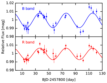
Figure 1: WiFSIP/STELLAR differential photometry of K2-18 taken in B (upper panel) and in R (lower panel). The solid curves show the best sine fit to the data. The star shows photometric variations with a semi-amplitude of 0.86% in the B band and 0.69% in the R band.

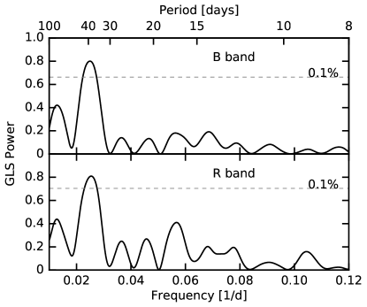
Figure 2: GLS periodogram of the B (upper panel) and R (lower panel) photometric data sets. The horizontal line indicates the 0.1% FAP level. Both data sets show a significant peak at $\sim 40$ days indicating the stellar rotation period.

To get a better estimate of the stellar rotation period, we fit both bands simultaneously with a sine wave function and forced both light curves to have the same frequency ($f_{BR}$) and phase ($\phi_{BR}$), but allowed the offsets ($\gamma_{B}$ and $\gamma_{R}$) and amplitudes ($A_{B}$ and $A_{R}$) to be different for each band. In total we fit for six parameters ($f_{BR}$, $\phi_{BR}$, $\gamma_{B}$, $\gamma_{R}$, $A_{B}$, and $A_{R}$) and performed a Markov Chain Monte Carlo (MCMC) using the emcee ensemble sampler (Foreman-Mackey et al., 2013). We adopted flat uniform priors for all parameters and estimate the rotation frequency to be $0.02524\pm 0.00032$ day^-1 ($39.63\pm 0.50$ days). This value is in agreement with the one estimated using the K2 photometry where Cloutier et al. (2017) derived a value of $38.6^{+0.6}_{-0.4}$ days using Gaussian processes and Stelzer et al. (2016) derived a value of 40.8 days using auto-correlation function (private comm.).

We estimated a photometric variability of $8.7\pm 0.5$ mmag in B and a smaller variability of $6.9\pm 0.5$ mmag in R. This difference is expected when the photometric variability is due to cool spots, since the contrast between the spots and the photosphere decreases at redder wavelengths. Figure 1 shows the photometric variations in the B filter (in blue) and the R filter (in red) and the best fit model. In Tables 4 and 5 we provide the differential photometry in B and R bands respectively.

3.2 Spectroscopic Indicators

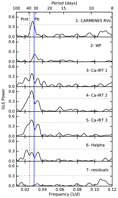
Figure 3: From top to bottom: GLS periodogram of the RVs, window function, the three Ca ii IRT lines, H$\alpha$ line, and the RV residuals. The blue solid line shows the orbital period of the planet, $P_{b}$, and the red dashed line indicates the stellar rotation period, $P_{\mathrm{rot}}$. The dashed horizontal lines show the 0.1% FAP. Excess power in the RVs close to the orbital period of the planet indicates the presence of the RV signal of the planet in the data. Prominent peaks in the Ca ii IRT and H$\alpha$ lines hint at the rotation period of the star.

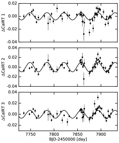
Figure 4: Time series of the three Ca ii IRT lines. The black curve shows the best fit to the data using a sinusoidal fit of which we estimate a period of $\sim$ 36 days.

The most common and widely used spectroscopic activity indicators can be divided into two different types: the chromospheric and the photospheric ones. The chromospheric activity indicators measure the excess of flux in the cores of e.g. Ca ii H&K, calcium infrared triplet (Ca ii IRT), Na i doublet, and H$\alpha$ lines. The core of these lines have their origin in the stellar chromosphere and hence they trace stellar magnetic activity. The photospheric activity indicators measure the degree of asymmetry in the line profile. The presence of spots on the photosphere distort the spectral lines and therefore periodic variability of the full width at half maximum (FWHM) and bisector span (BS) of the cross-correlation function (CCF) could indicate the presence of spots. Zechmeister et al. (2018) recently showed that the chromatic index is also an important photospheric indicator (see below).

The SERVAL pipeline provides the line indices of the Ca ii IRT, H$\alpha$, and Na i doublet. The three Ca ii IRT lines are centered at 8498.02 Å, 8542.09 Å, and 8662.14 Å, the H$\alpha$ line is centered at 6562.81 Å, and the Na i D lines are centered at 5889.95 Å and 5895.92 Å. The pipeline also computes the differential line width (dLW) and the chromatic RV index. The former is a measure of the relative change of the width of the average absorption line and the latter is a measure of the wavelength dependency on the RV. We refer the reader to Zechmeister et al. (2018) for a detailed description of how the various activity diagnostics are computed.

We performed a period search analysis using GLS to search for a significant periodicity that could be related to stellar activity. Figure 3 (panels 3 - 6) displays the periodograms of the indicators that show a significant peak. Although we inspected a wide range of frequencies, we only show the frequency range of interest that covers the stellar rotation frequency, the planetary frequency of the transiting planet, and the potential 9-day signal (see Section 4.3). All three Ca ii IRT indices show a clear dominant peak at $\sim 36$ days with FAP $=3\times 10^{-4}$, $<10^{-4}$, and $=10^{-4}$ for the Ca ii IRT 1, Ca ii IRT 2, and Ca ii IRT 3 lines respectively, which was determined via bootstrap. The H$\alpha$ periodogram shows three peaks at 29, 36, and 45 days with FAP $=3.7\times 10^{-3}$ at 36 days. The origin of the signal of both indicators is consistent, within the frequency resolution, with the rotational period of the star derived from photometry (Section 3.1). Similar to the photometric data, we fit the Ca ii IRT indices simultaneously with a sine wave function forcing them to have the same frequency and phase, but allowed the offsets and amplitudes to vary. Figure 4 shows the Ca ii IRT line indices along with the best fit sinusoidal model. The Na i doublet and dLW periodograms, however, are free from significant peaks even though the Na i lines were expected to be good activity indicators for early M-dwarfs (Gomes da Silva et al., 2011; Robertson et al., 2015). We report the data of the activity indicators in Table 6.

In addition to the indicators provided by SERVAL, we computed the CCF for each spectrum by cross-correlating the spectrum with a weighted binary mask that was built by co-adding all the observed spectra of the star itself. We selected around 4000 deep, narrow, and unblended lines, which were weighted according to their contrast and inverse FWHM. We computed one CCF for each spectral order and the final CCF was computed by combining all the individual CCFs according to signal-to-noise. A Gaussian function was fitted to the combined CCF. From this, the FWHM and bisector span were derived. A period analysis of the FWHM and bisector span does not show significant periods. The lines in a typical M dwarf spectrum are blended and, thus, may mask changes in the FWHM and bisector span, which could be the reason why these indicators do not show a variability. Another reason is probably the low projected rotational velocity of the star ($v\sin i$). Reiners et al. (2017) imposed an upper limit on $v\sin i$ at $2\,\mathrm{km\,s^{-1}}$. However, from the stellar radius and rotation period (Table 2), we estimate a true equatorial velocity $v$ of only $0.53\,\mathrm{km\,s^{-1}}$. The spot-BS relationship from Saar & Donahue (1997) predicts, for $v\sin i=0.53\,\mathrm{km\,s^{-1}}$, a bisector variability of 0.01 $\mathrm{m\,s^{-1}}$, which is too small to measure.

3.3 Photospheric vs Chromospheric Variations

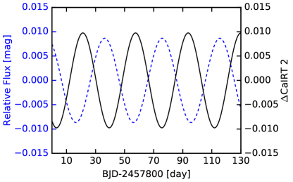
Figure 5: The blue dashed curve shows the photometric variability of K2-18 in the B band with a period of $\sim 40$ days. This is the same model shown in Figure 1. The solid black curve is the best sine fit of the Ca ii IRT 2 line with a period of $\sim 36$ days. During this time interval, the two curves are 180^∘ out-of-phase and show an anti-correlation between the photosphere and the chromosphere, especially in the second half of the data set.

The star shows photometric variability with a stellar rotation period of $39.63\pm 0.50$ days. The semi-amplitude is 0.87% in the B band and 0.69% in the R band. K2-18 also shows chromospheric variability in the Ca ii IRT and H$\alpha$ lines with a period consistent with the rotation period derived from photometry within the frequency resolution. Figure 5 shows the variations of the Ca ii IRT second index and the best fit model (solid black curve) and the photometric variability of K2-18 in the B band (dashed blue curve). There is an anti-correlation between the photometric and the chromospheric variability. The chromosphere shows variations which are 180^∘ out-of-phase with the photosphere. Similar trends are seen with the first and third Ca ii IRT indices and the H$\alpha$ line. This demonstrates that for high Ca ii emission values, a minimum in the photometric light curve is observed. This is expected if active chromospheric regions are present on top of a photospheric spot. This is not the first time that an anti-correlation between the chromosphere and photosphere of M dwarfs is observed. Bonfils et al. (2007) reported an anti-correlation for GJ 674, which is also an early M2.5 dwarf. It would be worth checking whether the anti-correlation will hold for late M dwarfs.

We conclude that K2-18 is a moderately active star and there is an anti-correlation between the photospheric and chromospheric variations, which is consistent with the previous results of Radick et al. (1998) for younger more active stars. Finally, although H$\alpha$ is a good activity indicator (Kürster et al., 2003; Hatzes et al., 2015; Robertson et al., 2015; Jeffers et al., 2018), the Ca ii IRT lines show a significantly stronger peak compared to H$\alpha$. Ca ii IRT are thus good chromospheric activity proxies (see discussion by Martin et al. (2017)) and provide a promising approach to detect stellar activity signals in M dwarfs, where the signal-to-noise is too low to measure Ca ii H&K lines, especially for mid and late M dwarfs. This is also in agreement with the findings of Robertson et al. (2016).

4 Radial Velocity Analysis

4.1 Periodogram Analysis of the RVs

Benneke et al. (2017) analysed the K2 and Spitzer light curves and derived an orbital period of $P=32.939614^{+0.000101}_{-0.000084}$ days. To ensure that we have detected the planet signal with high significance, we performed a periodogram analysis for the RVs obtained with CARMENES-VIS. The RV measurements show a peak at 34.97 days with a FAP $<10^{-4}$ (Figure 3, panel 1). This peak is approximately the mean of the planetary orbital frequency and the stellar rotation frequency (0.02524 day^-1), as measured in Section 3.1. The peak in the periodogram is therefore not centered at the orbital period of the planet but is shifted halfway between the stellar rotation frequency and the planetary orbital frequency. This shows that the RVs are contaminated by stellar activity, which is conceivable since the star is moderatively active (Section 3).

To assess the false alarm probability (FAP) of the planetary signal and, hence, to confirm the detection of the planet, we applied the bootstrap randomization technique. Unlike the previous analysis where we computed the GLS for the randomly shuffled data set (see Section 3.1), this time we fitted an adapted model to the randomized data points. The model employed the known ephemeris of the planet from Benneke et al. (2017), assumed zero eccentricity, and had only the RV semi-amplitude $K_{b}$ and the RV zero point (offset) as free parameters. We performed this 100,000 times and found that the FAP to infer a $K_{b}$ amplitude as large as (or larger than) the one estimated from the original data is $<10^{-5}$ and the FAP to get a $\chi^{2}$ as small as (or smaller than) the one from the original fit and finding at the same time that $K_{b}$ is positive is also $<10^{-5}$. This ensures that given the known ephemeris of the planet, we are confident that there is a signal at the known ephemeris, which can be a combination of the planet and activity signals. In Section 4.2 we address several tests that we performed to check whether the RVs and, therefore, the planetary amplitude is affected by activity.

Signals that are sampled at discrete times can produce fake signals in the periodogram that are due instead to observational patterns. In order to check for periodicities due to sampling, we applied the GLS on the window function (WF), which is a periodogram analysis of the observation times. The GLS shows a peak at 32.2 days (Figure 3, panel 2) which is very close to the orbital period of the planet. The reason for that peak is because we aimed to observe the star on a daily basis. However, some nights were lost due to bad weather and more importantly during dark nights, roughly for a couple of lunar cycles, another instrument was mounted on the telescope and no observations were carried out with CARMENES. This pattern could have caused the peak in the WF which is close to the lunar synodic cycle.

The presence of a peak in the WF would lead to the detection of the wrong frequency when there is a signal in the data. Dawson & Fabrycky (2010) showed that the reported periods of 55 Cnc e and HD 156668 b from their respective discovery papers were actually wrong and affected by daily aliases. In the case of K2-18 b, first we have evidence that the star is moderately active (Section 3) and, as a result, we anticipate the presence of a signal in the RVs close to the stellar rotation frequency. Second, the planet transits (Montet et al., 2015; Benneke et al., 2017) and, therefore, we expect another signal in the data close to the orbital period of the planet. However, the proximity of the stellar rotation frequency to the planetary orbital one makes separating them challenging, since the frequencies are not resolved given the time span of the data set.

Given the presence of the peak in the WF and assuming the presence of one signal in the data (either the planetary signal or the stellar rotational period), is it possible to retrieve the signal at the right frequency? To answer this question, we generated a single synthetic sinusoidal signal sampled at times identical to the real RVs. The uncertainty of every point corresponded to the uncertainties derived from the RVs. We generated two different sets, each with an amplitude of 3 $\mathrm{m\,s^{-1}}$, one set using the stellar rotation frequency and a second set using the planetary frequency. Finally, for the synthetic data generated using the rotational frequency, instead of fixing the phase, we covered a grid of phases $\left[-\pi,-0.9\pi,...,\pi\right]$. For the planetary signal we assumed that the phase is well constrained. We then did a periodogram analysis for each set and could recover a peak at the true frequency. This test shows that even though the WF shows a peak, we can still retrieve the signal at the right frequency (planet frequency or the stellar rotation frequency) given the data sampling. Hence, the data set is not affected by aliases

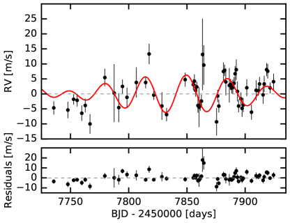
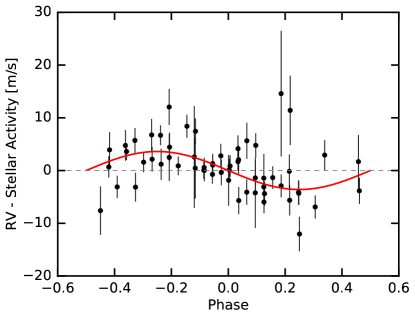
Figure 6: Left: CARMENES-VIS RVs modeled with a circular Keplerian signal of K2-18 b plus stellar activity modeled with a periodic sine function (red line), and the residuals to the best-fit model. Right: Phase-folded activity-corrected RVs along with the best-fit planetary model.

In short, the planet’s orbital period is 32.94 days (Benneke et al., 2017) and the stellar rotation period is $\sim 40$ days. The RVs are not only affected by activity but the WF also shows a peak close to 32.2 days, caused by observational patterns in the way the data was sampled. Previous studies (Robertson & Mahadevan, 2014; Vanderburg et al., 2016) showed the difficulty in detecting RV planets in orbits close to the stellar rotation period. Hatzes (2013) and Rajpaul et al. (2016) demonstrated that the WF can give rise to fake signals in the periodogram that mimicked the presence of a planet around $\alpha$ Cen B which was reported by Dumusque et al. (2012). In the case of K2-18 b, the planet transits and hence its existence is undeniable. However, a closer look at the WF is needed to check whether the RV signal of the planet is present in the data. This case demonstrates the difficulty in detecting non-transiting low-mass planets not only at orbits close to the stellar rotation period but also when observational patterns are present in the data.

4.2 Orbital Analysis of K2-18 b

We performed joint modeling of the photometric light curves obtained with STELLA and the RV measurements. Similar to Section 3.1, we modeled the photometric data of both bands with a sine wave function and fit for $f_{BR}$, $\phi_{BR}$, $\gamma_{B}$, $\gamma_{R}$, $A_{B}$, and $A_{R}$. We adopted uniform priors for the phase and offsets of the stellar photometric variability. For $f_{BR}$, $A_{B}$, and $A_{R}$ we adopted Gaussian priors centered at $0.02524$ day^-1, 8.7 mmag, and 6.9 mmag, respectively and with a standard deviation of 0.00032 day^-1 and 0.5 mmag for both amplitudes (see Section 3.1). We fit the RV measurements with a Keplerian model assuming a circular orbit ($e$ = 0) and using the combined K2 and Spitzer ephemeris, i.e. we fixed the mid-transit time $T_{0}$ and $P_{b}$ to the values derived photometrically by Benneke et al. (2017) since these parameters are tightly constrained. We accounted for stellar activity in the RV data by assuming that it has a sinusoidal function whose frequency is constrained from the photometric light curves. We let the phase of the stellar activity $\phi_{\mathrm{act}}$ free, and thus fit for the phase, amplitude $K_{\mathrm{act}}$, and frequency $f_{BR}$ of the stellar activity. We adopted non-informative priors for the offset, $\phi_{\mathrm{act}}$, $K_{\mathrm{act}}$, and $K_{b}$. The joint analysis was then performed using emcee (Foreman-Mackey et al., 2013) and in total we fit for 10 parameters: 6 parameters for the photometric data (mentioned above) and 5 parameters for the RV data ($\gamma$, $K_{b}$, $\phi_{\mathrm{act}}$, $K_{\mathrm{act}}$, and $f_{BR}$); the stellar rotation frequency is the same in both data sets.

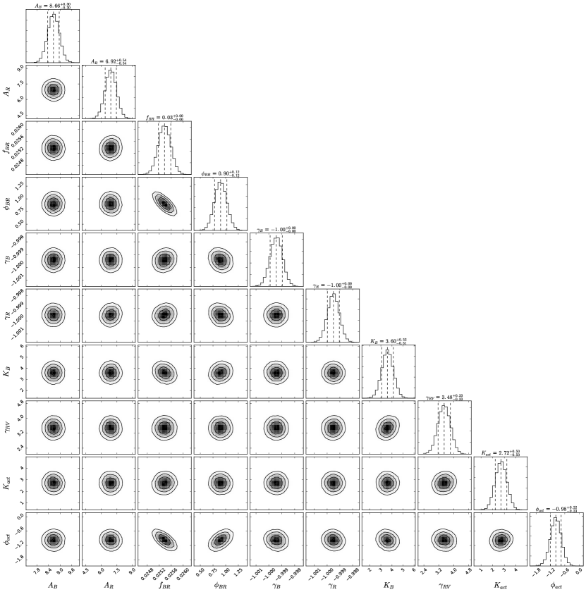
Figure 13: The marginalized posterior distributions on the model parameters from the joint analysis of the photometry and CARMENES RV measurements.

The best fit model gave a planetary semi-amplitude of $K_{b}=3.60^{+0.53}_{-0.51}$ $\mathrm{m\,s^{-1}}$ and a stellar activity semi-amplitude of $K_{\mathrm{act}}=2.72\pm 0.50$ $\mathrm{m\,s^{-1}}$, corresponding to a planetary mass of $M_{b}=9.07^{+1.58}_{-1.49}\,M_{\oplus}$, using $M_{*}=0.359\pm 0.047$ $M_{\odot}$. Figure 13 shows the joint and marginalized posterior constraints on the model parameters. Using the transit depth , $R_{\mathrm{b}}/R_{*}$, and stellar radius, $R_{*}$, as reported in Benneke et al. (2017) and provided in Table 2, we derive a planetary radius $R_{b}=2.37\pm 0.22\,R_{\oplus}$, this corresponds to a planetary density of $\rho_{b}=4.18^{+1.71}_{-1.17}$ g cm^-3. The $v\sin i$ and spot filling factor estimated from photometry yield an RV semi-amplitude of 2.7 $\mathrm{m\,s^{-1}}$ for spots using the relationship by Hatzes (2002), which is in excellent agreement with the one estimated using the RV data. The planetary semi-amplitude value is consistent with the one derived using HARPS RVs by Cloutier et al. (2017) at the 1-sigma level. The best fit model and the phased RVs are shown in Figure 6. We report the stellar and planetary parameters used in this study and the median values of all the parameters, along with the $16^{\mathrm{th}}$ and $84^{\mathrm{th}}$ percentiles of the marginalized posterior distributions in Table 2.

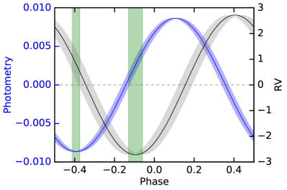
Figure 7: Phase-folded photometric light curve in the B band (blue) and RV signal due to activity (black), along with their 1$\sigma$ uncertainties. To aid the eye, the minima of both curves are shaded in green. Within the error bars the phase shift between the two curves is 90^∘, as expected if the photometric and RV signals are due to cool spots crossing the visible stellar surface as the star rotates.

To further test whether the activity signal is due to cool spots, we compared the phase shift between the photometric light curve and the RV signal due to activity. Figure 7 shows the phase folded photometric light curve in the B band in blue and the RV signal in black. When the spot is at the center of the stellar surface (minimum in the photometric light curve), the contribution of the spot to the RV signal is close to zero. As the spot moves along the stellar surface to the receding redshifted limb (zero in the photometric light curve), the star appears to be blueshifted (minimum in the RV curve). Therefore, the phase shift is $\sim 90^{\circ}$. This is expected if the variations are due to cool spots, which is also consistent with the multi-wavelength photometry analysis (Section 3.1). This is only considering the flux effect of dark spots. In general, the RV variations in active regions are induced by two different physical processes: first the asymmetry in the stellar line profiles created by star spots and second the suppression of the convective blueshift effect due to the presence of strong magnetic fields that inhibit convection inside active regions. The convective blueshift effect could explain why the RV curve appears shifted a bit vertically at the minimum phase of the photometric lightcurve.

Even though the star shows periodic photometric variability, there is evidence that the chromosphere does not show strict periodic sine-like variability (see Section 4.3 and Figure 4, where some points deviate from the best fit curve, especially Ca ii IRT 1 and Ca ii IRT 3). Therefore, modelling the RV signal of stellar activity by a periodic sinusoidal function might not be the best approach. However, we next argue that the derived planetary semi-amplitude is not dependent on our choice of the model used to account for stellar activity. We performed several tests to check this dependency. First, following Baluev (2009), we accounted for stellar activity by adding a constant white noise term often referred to as the RV jitter term, $\sigma_{\mathrm{jitter}}$. The jitter term is treated as an additional source of Gaussian noise with variance $\sigma^{2}_{\mathrm{jitter}}$ and is added in quadrature to the estimated RV uncertainties (Ford, 2006). We derived a planetary semi-amplitude $K_{b}=3.38^{+0.75}_{-0.76}$ $\mathrm{m\,s^{-1}}$ and an RV jitter $\sigma_{\mathrm{jitter}}=3.02^{+0.57}_{-0.53}$ $\mathrm{m\,s^{-1}}$. The planetary semi-amplitude derived using this model is in agreement with the one derived previously, within the 1-sigma error bars.

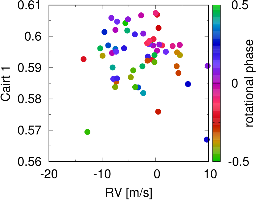
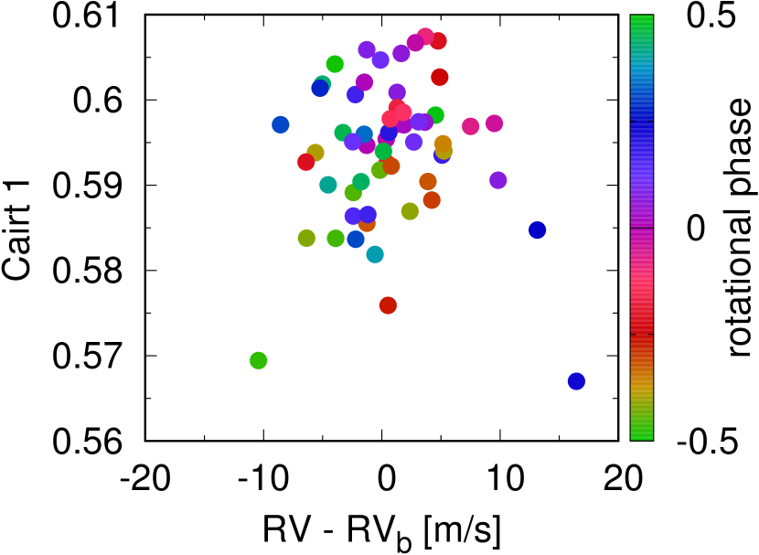
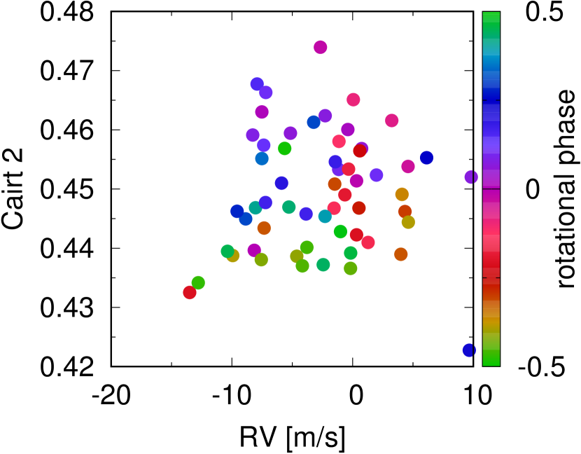
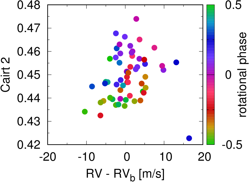
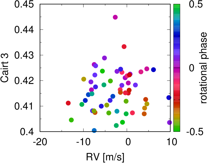
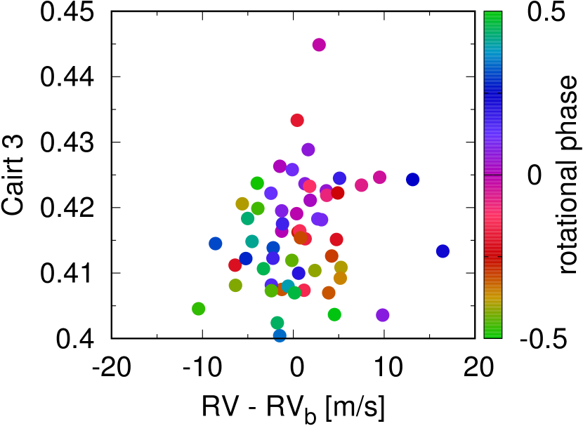
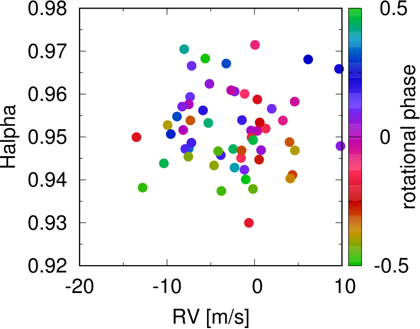
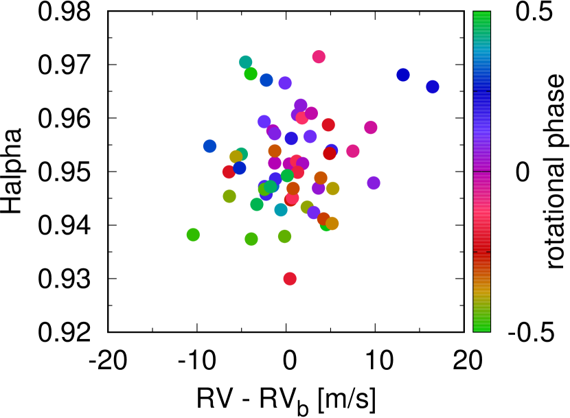
Figure 12: Upper panels: measured RVs plotted against various stellar activity indicators phase folded using the stellar rotation period of 39.63 days. Lower panels: same as the upper panels but after subtracting the planetary signal. None of the activity indicators show a statistically significant linear or circular correlation with the raw RVs or the residuals.

Second, to check whether the RVs are affected by stellar activity, we looked for correlations between the raw RVs and the various activity indicators mentioned in Section 3.2. The upper panels in Figure 12 in the Appendix A show the measured RVs plotted against the activity indicators and color coded according to the stellar rotational phase. We did not find a linear correlation between any of these quantities and the measured RVs. However, there is a slight indication that the color coded data points follow a circular path, especially for Ca ii IRT 2, but not with high significance. We further repeated the same analysis after the removal of the planetary signal and still did not find any significant correlations with the activity indicators. The results are shown in the lower panel of Figure 12. Despite detecting a signal close to the stellar rotational period in both the RVs and the Ca ii IRT lines, no evident linear or circular correlation is seen, indicating that the relation is quite complex.

Third, we ignored activity and fit the RVs with a single Keplerian signal and fixed $T_{0}$ and $P_{b}$ to the known photometric values. We estimated a planetary semi-amplitude $K_{b}=3.35\pm 0.47$ $\mathrm{m\,s^{-1}}$ which is also in agreement with the previous results. We further divided the data set into two, each containing 29 data points, and repeated the same analysis for the first and second half of the data. We found similar planetary semi-amplitudes in both cases and the values are given in Table 1.

As a final test, we looked at the RV measurements in the red and blue orders of CARMENES-VIS. If the RVs are dominated by activity due to active regions on the stellar surface, then the planetary semi-amplitude in the blue part of the spectrum should be more affected by activity whereas the red part should be less affected. As a result, if the star is active, a single Keplerian fit to the data should yield different planetary semi-amplitudes for different orders. The RV measurements for K2-18 are available at 42 orders. We calculated an RV weighted mean average for the first and second half of the orders, which we will refer to as the blue RVs and as the red RVs respectively and are reported in Table 6. The blue orders cover the wavelength range from 561 to 689 nm, whereas the red orders cover the range from 697 to 905 nm. We also ignored activity and fit separately the blue and red RVs with a Keplerian model with $T_{0}$ and $P_{b}$ fixed. We did this analysis for the full CARMENES-VIS data set, the first half, and the second half. So in total we repeated this analysis six times, all of which yielded similar planetary semi-amplitudes within the error bars. The values are reported in Table 1, where we denote the original full wavelength coverage RVs as full-$\lambda$ RVs. We conclude that the RVs are not dominated by stellar activity, and that the estimation of the planetary semi-amplitude is robust and does not depend on the choice of model used to account for stellar activity.

We also computed the results of Table 1 using a Keplerian model plus a sinusoidal model to account for activity, where we fit for the stellar rotation frequency. We find that the planetary semi-amplitude is consistent within 1-sigma when computed for the full data, first half, and second half for the full spectral coverage, the red, and blue orders with one exception, the planetary amplitude computed for the second half in the red order. However, the value is in agreement at the 2-sigma level. Even though we expect the activity semi-amplitudes to be different in different orders, the semi-amplitudes derived are consistent either at the 1-sigma or at the 2-sigma level. This could be explained by the low amplitude signals in both order ranges, which are on the order of $2.7\pm 0.73$ $\mathrm{m\,s^{-1}}$ i.e. a higher precision would be required to differentiate between the activity semi-amplitudes in different orders.

Table 1: The planetary semi-amplitudes $K_{b}$ derived for the full, first, and second half of the data set using the full-$\lambda$ RVs, the blue RVs, and the red RVs.

$K_{b}\,(\mathrm{m\,s^{-1}})$	Full Set	First Set	Second Set
Full-$\lambda$ RVs	3.35 $\pm$ 0.47	3.23 $\pm$ 0.66	3.10 $\pm$ 0.68
Blue RVs	3.46 $\pm$ 0.55	3.71 $\pm$ 0.79	$2.71^{+0.80}_{-0.77}$
Red RVs	3.29 $\pm$ 0.46	2.77 $\pm$ 0.65	3.44 $\pm$ 0.64

4.3 Search for a Second Planet

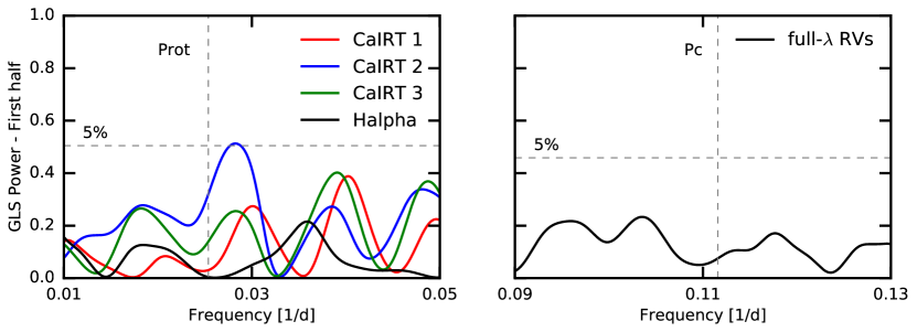
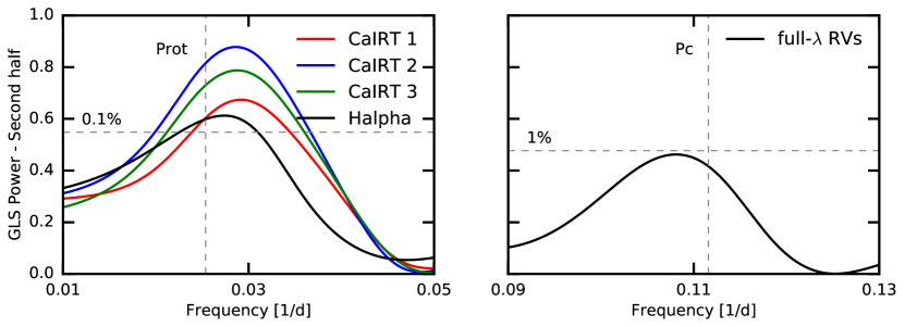
Figure 8: Periodograms of the first (top panels) and second (bottom panels) halves of the Ca ii IRT and H$\alpha$ lines (left panels) and CARMENES-VIS RVs (right panels). The dashed lines on the left and right show the stellar rotational period $P_{\mathrm{rot}}$ and the claimed period of the inner planet $P_{c}$ respectively. The signal of the inner planet is only present in the second half of the data set when all the spectroscopic indicators show a single significant signal at $P_{\mathrm{rot}}$.

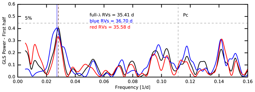
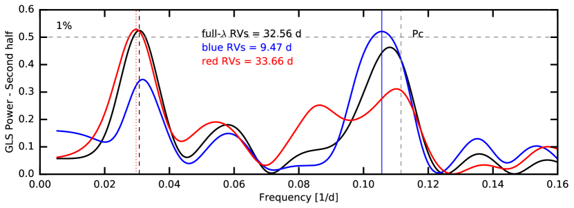
Figure 9: Periodograms of the first (top panel) and second (bottom panel) halves of the data set of the full-$\lambda$ RVs, blue RVs, and red RVs. The dashed, solid, and dotted lines indicate the peak with the highest GLS power for the full-$\lambda$ RVs, blue, and red RVs, respectively. The signal of the inner planet $P_{c}$ is only prominent in the second half of the data set when the star shows high level of activity.

Cloutier et al. (2017) used 75 HARPS RV measurements spanning approximately three seasons of observations to estimate the mass of K2-18 b and to search for additional planetary signals. They reported a non-transiting planet, K2-18 c, with a period of $8.962\pm 0.008$ days and a semi-amplitude of $4.63\pm 0.72$ $\mathrm{m\,s^{-1}}$. The signal of K2-18 c is stronger than K2-18 b (see Figure 2 in Cloutier et al. (2017)).

We searched for the signal of the second planet in the CARMENES-VIS data set. As mentioned in Section 4, the periodogram only shows one strong peak at 34.97 days, the combined signal of the $\sim 33$-day period planet and the stellar rotation period. The second strongest peak is around 9 days with a FAP $>$ 5% and significantly weaker than in the HARPS data. We then subtracted the signal of the 33-day period planet and stellar activity from the RVs and performed again a period analysis. We still did not find a strong signal at the period of the supposed second (inner) planet (Figure 3, panel 7).

In order to examine whether the absence of the 9-day signal in the CARMENES-VIS data set is due to bad sampling, we generated a synthetic RV data set assuming that there are two planets in the system and using the real observing times of CARMENES. We set the values of the orbital period, semi-amplitude, and time of inferior conjunction of both planets as derived by Cloutier et al. (2017): $P_{b}=32.93963$ days, $P_{c}=8.962$ days, $K_{b}=3.18$ $\mathrm{m\,s^{-1}}$, $K_{c}=4.63$ $\mathrm{m\,s^{-1}}$, $T_{0,b}=2457264.39157$ BJD, and $T_{0,c}=2457264.55$ BJD. We further assumed that the uncertainty is the sum of the observational error and a random noise (drawn from a normal distribution centered at 0 and a standard deviation of 0.25 $\mathrm{m\,s^{-1}}$) to attribute to the stellar jitter determined by Cloutier et al. (2017). We then did a periodogram analysis and could recover an extremely strong peak at 8.98 days with a FAP $<0.1\%$. This shows that our analysis is not affected by poor time sampling.

We also examined whether the 9-day signal could be caused by stellar activity, since the period is near the fourth harmonic of the stellar rotation period ($39.63$ days – Section 3; Cloutier et al., 2017). We divided the full CARMENES-VIS data set into two, each consisting of 29 data points, and did a periodogram analysis for each set of the RVs, Ca ii IRT, and H$\alpha$ lines. Figure 8 shows the periodograms for both data sets. The upper left and upper right panels show the periodograms of the activity indicators and RVs respectively for the first half of the CARMENES-VIS data set. Similarly, the lower panels show the periodograms for the second half of the data set. The dashed line in the periodograms of the activity indicators shows the stellar rotation period, $P_{\mathrm{rot}}$, while the dashed line in the RV periodograms indicates the period of the inner planet, $P_{c}$, as estimated by Cloutier et al. (2017). Note that for the activity indicators only the periodogram region near the rotation period is shown, whereas for the RVs only the region around the 9-day signal is displayed. The different levels of FAPs are indicated in the plot. The first half of the RV data set does not show a power at the orbital period of the supposed inner planet. That is also true when the Ca ii IRT and H$\alpha$ lines do not show a consistent peak. The second Ca ii IRT index is the only indicator that shows a somewhat stronger peak with a FAP $\sim 1$%. The other indicators do not show a prominent peak and notably H$\alpha$ shows no power at the stellar rotation period. The signal of the 9-day period appears only in the second half of the RV data set, which occurs at the same time when all the Ca ii IRT and H$\alpha$ lines show a prominent peak at the stellar rotation period with a FAP $<$ 0.1%, demonstrating that the level of activity increased in this set. This indicates that the signal of the 9-day planet is absent when the star is less active and is present only when the level of activity increases significantly. We thus conclude that the presence of the 9-day signal correlates with the Ca ii IRT and H$\alpha$ lines.

This is further illustrated in Figure 9, which shows the periodograms of the full-$\lambda$ RVs and the blue and red RVs of CARMENES-VIS, which are calculated as explained in Section 4.2. The periodogram for the blue RVs is shown in blue, for the red RVs in red, and for the full-$\lambda$ RVs in black. The legend indicates the period with the highest power for the different sets of RVs. The blue, red, and full-$\lambda$ RVs show a single peak in the first half of the data set (upper panel) close to 36 days. In the second half, interestingly the periodogram of the blue RVs shows the highest GLS power close to 9 days, while the red and full-$\lambda$ RVs show the highest power close to the orbital period of the 33-day period planet. This further demonstrates that when the level of stellar activity increased, the blue RVs show a period at the fourth harmonic of the stellar rotation period while the red RVs do not. This is in line with the notion that RV variations due to photometric star spots are wavelength dependent and more prominent in the blue part of the spectrum, while the variations get smaller at redder wavelengths (Reiners et al., 2010). On the other hand, the RV variation of a planetary signal is wavelength independent and should be constant at all wavelengths. This shows the importance of multi-wavelength RV measurements to differentiate planetary from stellar activity signals.

Table 2: Stellar and planetary parameters for the system K2-18.

Parameter		Value
Stellar parameters
$\qquad P_{\mathrm{rot}}$ [days]		39.63 $\pm 0.50$
$\qquad M_{*}$ [$M_{\odot}$]		0.359 $\pm 0.047$
$\qquad R_{*}$ [$R_{\odot}$]		0.411 $\pm 0.038$
$\qquad T_{*}$ [K]		3457 $\pm 39$
[Fe/H] [dex]		0.12 $\pm 0.16$
Transit parameters
$\qquad R_{\mathrm{b}}/R_{*}$ [%]		5.295${}^{+0.061}_{-0.059}$
$\qquad T_{0}$ [BJD]		2457264.39144${}^{+0.00059}_{-0.00066}$
$\qquad P_{b}$ [d]		32.939614${}^{+0.000101}_{-0.000084}$
$\qquad R_{\mathrm{b}}$ [$R_{\oplus}$]		2.37$\pm 0.22$
$\qquad i$ [deg]		89.5785${}^{+0.0079}_{-0.0088}$
		Models
	Planet only	Planet + sine	Planet + jitter
Radial Velocity parameters
$\qquad K_{b}$ $\left[\mathrm{m\,s^{-1}}\right]$	3.35 $\pm 0.47$	$3.60^{+0.53}_{-0.51}$	$3.38^{+0.75}_{-0.76}$
$\qquad K_{\mathrm{act}}$ $\left[\mathrm{m\,s^{-1}}\right]$	…	$2.72\pm 0.50$	…
$\qquad\sigma_{\mathrm{jitter}}$ $\left[\mathrm{m\,s^{-1}}\right]$	…	…	$3.02^{+0.57}_{-0.53}$
$\qquad e$	0 (fixed)	0 (fixed)	0 (fixed)
Planet parameters
$\qquad a$ [au]	0.1429${}^{+0.0060}_{-0.0065}$	0.1429${}^{+0.006}_{-0.0065}$	0.1429${}^{+0.006}_{-0.0065}$
$\qquad M_{\mathrm{b}}$ [$M_{\oplus}$]	8.43${}^{+1.44}_{-1.35}$	9.06${}^{+1.58}_{-1.49}$	8.49${}^{+2.08}_{-1.97}$
$\qquad T_{\mathrm{eq}}$ [K]	$283\pm 15$	$283\pm 15$	$283\pm 15$
$\qquad\rho_{\mathrm{b}}$ [g cm-3]	$3.89^{+1.58}_{-1.08}$	$4.18^{+1.71}_{-1.17}$	$3.90^{+1.77}_{-1.24}$

Notably, in the second half of the data set, when the star is relatively more active, the red and full-$\lambda$ RVs show peaks much closer to the the orbital period of the planet and are not shifted in value toward that of the stellar rotation. It seems the contribution of activity to the RVs appears near the fourth harmonic of the stellar rotation period and this set shows a clean planetary signal.

We conclude that, although we found evidence of the second planet signal announced recently by Cloutier et al. (2017), the peak is not significant in the CARMENES-VIS data set with a FAP $>$ 5%. The signal is also time and color variable and correlates with stellar activity. Given the sampling and the time baseline of our observations, we conclude we do not have enough evidence to confirm the presence of the second inner planet and there is a strong indication that the signal is intrinsic to the star. This also could explain why no transits were observed by K2 (Cloutier et al., 2017), although this can also be explained by misaligned orbits.

5 Joint HARPS and CARMENES Analysis

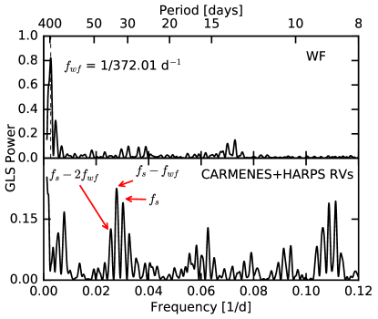
Figure 10: Periodogram of the WF (top) and RVs for the combined HARPS and CARMENES data set (bottom). The WF shows a significant peak at the sidereal year. The aliases of the planetary signal are indicated by the red arrows.

In this Section, we combine both the HARPS and CARMENES-VIS data sets to refine the parameters of the system, in particular to put constraints on the eccentricity. The joint HARPS (75 observations) and CARMENES-VIS (58 observations) data sets contain a total of 133 RV measurements with a time baseline of 807 days. A periodogram analysis for the WF of the combined set reveals a peak at $\sim$ 372 days (Figure 10, upper panel). This is expected since the data set spans three seasons with gaps in between. However, if there is a signal in the raw RVs at frequency $f_{s}$, then in the periodogram, aliases will likely appear at $f_{\mathrm{alias,n}}$ = $f_{s}+nf_{\mathrm{WF}}$, where $n$ is an integer and $f_{\mathrm{WF}}$ is the frequency at which the WF shows a peak (also known as the sampling frequency) (Dawson & Fabrycky, 2010). Considering that the RV signal due to the transiting planet is present in the data, then $f_{\mathrm{alias,1}}=1/32.9396-1/372.01=0.02767$ day^-1 ($\sim$ 36.14 days). For $n=2$, $f_{\mathrm{alias,2}}=0.02498$ day^-1 ($\sim$ 40.03 days). This means that an alias of the orbital frequency of the planet is right at the stellar rotation frequency. Similarly, the aliases of the stellar rotation frequency are also approximately at 33 and 36 days. It is a coincident that the alias of one signal is close to the real frequency of the other signal. It is also by chance that the aliases of both signals meet at 36 days. So these aliases interfere and give a higher GLS power at this frequency. The aliases are shown in the lower panel of Figure 10.

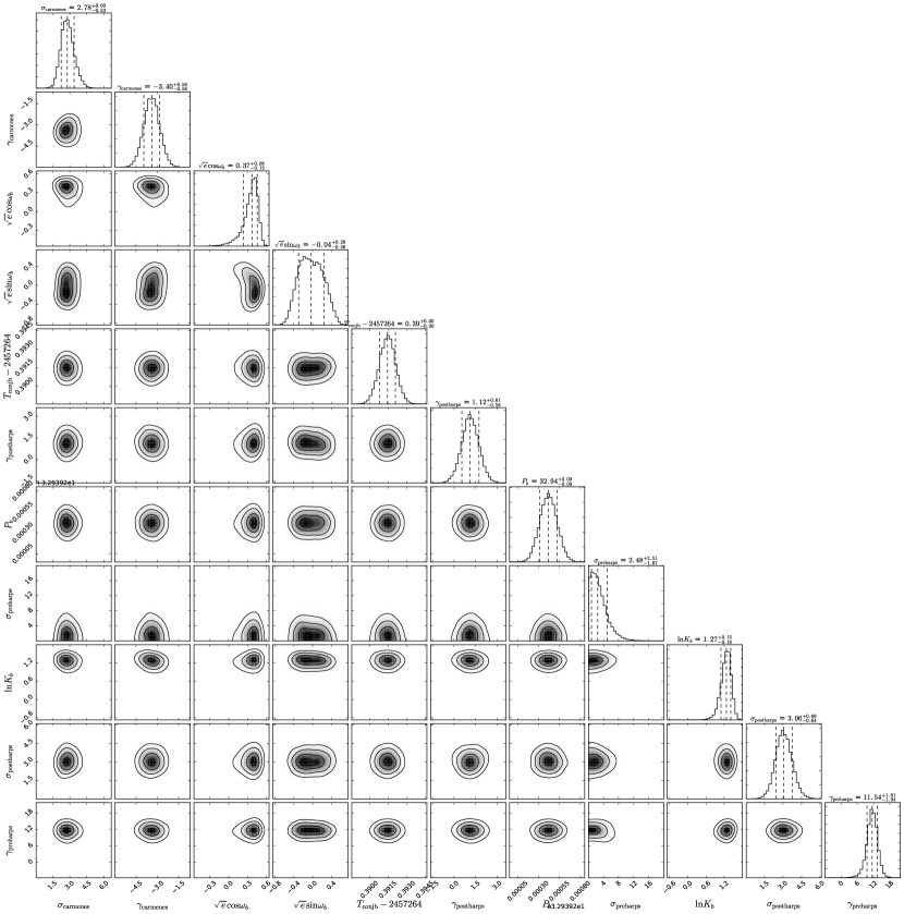
Figure 14: The marginalized posterior distributions on the model parameters of the RV measurements using CARMENES and HARPS data.

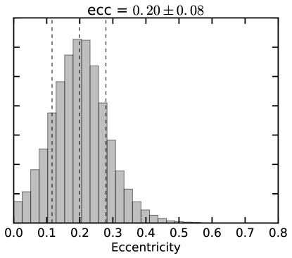
Figure 15: The posterior distribution of $e$ calculated from $\sqrt{e}\cos\omega_{b}$ and $\sqrt{e}\sin\omega_{b}$. The vertical lines show the 16^th, 50^th, and 84^th percentile.

We performed a Keplerian fit for the combined HARPS and CARMENES-VIS RVs using the publicly available python package RadVel (Fulton et al., 2018). RadVel is capable of modeling RV data taken with different instruments and uses a fast Keplerian equation solver written in C and the emcee ensemble sampler (Foreman-Mackey et al., 2013). The optical fibres of the HARPS spectrograph were upgraded in June 2015 (Lo Curto et al., 2015). Consequently, this affected the radial velocity offset and therefore we treated the data taken pre- and post-fibre upgrade separately by accounting a different velocity offset for each data set ($\gamma_{\mathrm{preHARPS}}$ and $\gamma_{\mathrm{postHARPS}}$). We account for stellar activity by adding an RV jitter term. Three independent jitter terms ($\sigma_{\mathrm{preHARPS}}$, $\sigma_{\mathrm{postHARPS}}$, $\sigma_{\mathrm{CARMENES}}$) were added in quadrature to the formal error bars of each instrument and were allowed to vary. We followed Ford (2005) and fit for $\sqrt{e}\cos\omega$ and $\sqrt{e}\sin\omega$ instead of the eccentricity $e$ and argument of periastron $\omega$ to increase the rate of convergence. We thus fit for eleven parameters: the planetary semi-amplitude $K_{b}$, $\sqrt{e}\cos\omega$, $\sqrt{e}\sin\omega$, planetary orbital period $P_{b}$, time of conjunction $T_{c}$, the velocity offsets for the CARMENES, HARPS pre-fibre, and HARPS post-fibre upgrade, $\gamma_{\mathrm{CARMENES}}$, $\gamma_{\mathrm{preHARPS}}$, and $\gamma_{\mathrm{postHARPS}}$, and for $\sigma_{\mathrm{preHARPS}}$, $\sigma_{\mathrm{postHARPS}}$, and $\sigma_{\mathrm{CARMENES}}$. We assign Gaussian priors on $P_{b}$ and $T_{c}$, adopt uniform uninformative priors on the jitter and offset terms and measure $e=0.20\pm 0.08$ and $K_{b}=3.55^{+0.57}_{-0.58}$ $\mathrm{m\,s^{-1}}$. This translates into a planetary mass $M_{\mathrm{b}}=8.92^{+1.70}_{-1.60}\,M_{\oplus}$, consistent with the previous analysis using only the CARMENES-VIS data set (Section 4.2). The median values and the 68% credible intervals are reported in Table 3. The joint and marginalized posterior constraints on the model parameters are shown in Figure 14 and Figure 15 shows the eccentricity distribution.

Table 3: Orbital and planetary parameters for the system K2-18 b for the combined HARPS and CARMENES-VIS data sets

Parameter	Value
Orbital Parameters
$\qquad T_{0}$ [BJD]	$2457264.39144\pm 0.00065$
$\qquad P_{b}$ [d]	$32.939623^{+0.000095}_{-0.000100}$
$\qquad K_{b}\left[\mathrm{m\,s^{-1}}\right]$	$3.55^{+0.57}_{-0.58}$
$\qquad e_{b}$	$0.20\pm 0.08$
$\qquad\omega_{b}$ [rad]	$-0.10^{+0.81}_{-0.59}$
Planetary Parameters
$\qquad R_{\mathrm{p}}$ [$R_{\oplus}$]	2.37$\pm 0.22$
$\qquad i$ [deg]	89.5785${}^{+0.0079}_{-0.0088}$
$\qquad a$ [au]	0.1429${}^{+0.006}_{-0.0065}$
$\qquad M_{\mathrm{b}}$ [$M_{\oplus}$]	$8.92^{+1.70}_{-1.60}$
$\qquad T_{\mathrm{eq,b}}$ [K]	$284\pm 15$
$\qquad\rho_{\mathrm{b}}$ [g cm-3]	$4.11^{+1.72}_{-1.18}$
Other Parameters
$\qquad\gamma_{\mathrm{CARMENES}}\left[\mathrm{m\,s^{-1}}\right]$	$-3.40\pm 0.56$
$\qquad\gamma_{\mathrm{preHARPS}}\left[\mathrm{m\,s^{-1}}\right]$	$656.4^{+1.8}_{-1.9}$
$\qquad\gamma_{\mathrm{postHARPS}}\left[\mathrm{m\,s^{-1}}\right]$	$653.86^{+0.61}_{-0.59}$
$\qquad\sigma_{\mathrm{CARMENES}}\left[\mathrm{m\,s^{-1}}\right]$	$2.78^{+0.61}_{-0.53}$
$\qquad\sigma_{\mathrm{preHARPS}}\left[\mathrm{m\,s^{-1}}\right]$	$2.5^{+2.5}_{-1.7}$
$\qquad\sigma_{\mathrm{postHARPS}}\left[\mathrm{m\,s^{-1}}\right]$	$3.06^{+0.69}_{-0.64}$

6 Discussion

Using the CARMENES-VIS data only, we detected K2-18 b with a semi-amplitude of $K=3.60_{-0.51}^{+0.53}$ $\mathrm{m\,s^{-1}}$, in agreement with the value estimated by Cloutier et al. (2017) using data taken with HARPS. We then combined the CARMENES-VIS and HARPS data sets to refine the planetary parameters, particularly to put constraints on the eccentricity. We derived a semi-amplitude of $K_{b}=3.55^{+0.57}_{-0.58}$ $\mathrm{m\,s^{-1}}$ and eccentricity $e=0.20\pm 0.08$ indicating that the planet is on a slightly eccentric orbit. This implies a mass $M_{\mathrm{b}}=8.92^{+1.70}_{-1.60}\,M_{\oplus}$ that, combined with the radius estimate we derived in Section 4.2 $R_{\mathrm{b}}=2.37\pm 0.22\,R_{\oplus}$, leads to a bulk density of $\rho_{b}=4.18^{+1.71}_{-1.17}\,\mathrm{g\,cm^{-3}}$. However, the radius estimate could be affected by systematic errors due to stellar contamination (Rackham et al., 2018). Consequently, this leads to systematic errors in the derived density.

We put the parameters of K2-18 b in the context of discovered exoplanets of similar sizes and masses. Figure 11 shows the position of K2-18 b on the mass-radius diagram in comparison with the other discovered exoplanets with radii less than $4R_{\oplus}$, masses smaller than 32 $M_{\oplus}$, and with masses and radii determined with a precision better than 30%. Theoretical two-layer models obtained from Zeng et al. (2016) are overplotted. It can be seen that K2-18 b can have a composition consistent with $\sim$ 100% water (H₂O) or $\sim$ 50% H₂O and $\sim$ 50% rock (MgSiO₃) indicating that this planet could be water rich. However, it is well known that there is a wide range of possible compositions for a given mass and radius, all of which include low density volatiles such as water and H/He (Lopez et al., 2012; Jin & Mordasini, 2018). The radius of K2-18 b can be thus explained by a silicate and iron core along with a H/He envelope or with a water envelope. This is in agreement with Rogers (2015) and Wolfgang & Lopez (2015), who showed that most planets with radii larger than 1.6 R_⊕ are not rocky.

Transiting low-mass planets in the temperate zone of M stars are potential prime targets for detailed atmospheric characterization. K2-18 b lies in the temperate zone of its host star (Kopparapu et al., 2013, 2014) and receives stellar irradiation similar to Earth. In addition to that, the brightness of the star in the NIR ($J=9.8$ mag and $K=8.9$ mag) and its close distance makes K2-18 b a good candidate for detailed atmospheric characterization with observations of secondary transits. The James Webb Space Telescope will be able to simultaneously observe from 0.6 to 2.8 $\mu$m and thus can provide robust detections of water absorption bands in the NIR (if any) for this bright target.

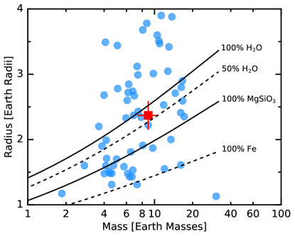
Figure 11: Mass-radius diagram for well characterized transiting exoplanets. K2-18 b (red square) and theroretical models (Zeng et al., 2016) are overplotted. The composition of the planet is consistent with 50% H₂0 and 50% MgSiO₃.

7 Conclusions

K2-18 b was first discovered as part of the K2 mission (Montet et al., 2015). Later, Benneke et al. (2017) confirmed the presence of the planet by detecting a third transit light curve of the same depth using Spitzer. We obtained contemporaneous photometric and spectroscopic observations to model jointly stellar activity and the Keplerian signal of K2-18 b. We found the stellar rotation period $P_{\mathrm{rot}}$ to be close to the planetary orbital period, in agreement with K2 photometry (Cloutier et al., 2017; Stelzer et al., 2016). The simultaneous photometric data along with the precise RV observations were a key to disentangle these two signals. Coincidentally, the window function also shows a peak close to the orbital period of the planet. We performed several tests to assess whether the RV signal due to the planet is detected in the RV data and to test whether stellar activity affects the determination of the planetary amplitude. Our analysis highlights the difficulty in detecting non-transiting low-mass planets in the presence of uneven sampling and, more importantly, when the planetary signal is close to the stellar rotation period.

Using data taken with HARPS, Cloutier et al. (2017) claimed that the system hosts two planets: ($i$) an outer planet, K2-18 b, with an amplitude of $K_{b}=3.18\pm 0.71$ $\mathrm{m\,s^{-1}}$, ($ii$) an inner non-transiting planet, K2-18 c, which has a higher signal compared to K2-18 b, and a period of $8.962\pm 0.008$ days. While the existence of K2-18 b is in agreement with results derived with the CARMENES-VIS data, the 9-day signal in our data set is not significant and only present in the blue part of the spectrum when the star is showing high activity levels. We thus believe that the signal is time and color variable, and is correlated with the chromospheric stellar activity. K2-18 c is mostly an artifact of stellar activity and not a bona fide planet. This analysis underscores the importance of multi-wavelength RV observations, in particular the value of comparing the blue and red orders of active stars to check the consistency of planetary signals across all orders of the Echelle spectrum.

Disentangling the signal of a low-mass planet from the stellar RV signal is still challenging. Following Vanderburg et al. (2016), we also encourage future studies to perform a combined analysis of simultaneous photometry, multi-wavelength RV observations, and analysis of the activity indicators to overcome these challenges and to test the reliability of signals present in the data.

Appendix A Additional Figures and Tables

Table 4: WiFSIP photometry in the Johnson B filter.

BJD $-2450000$	$\Delta B$	$\sigma_{B}$
(days)	(mag)	(mag)
7812.628906	0.9934	0.0023
7813.632812	0.9894	0.0020
7815.636719	0.9928	0.0022
7816.625000	0.9889	0.0028
7817.597656	0.9896	0.0062
7818.628906	0.9965	0.0024
7819.585938	0.9886	0.0052
7833.562500	1.0046	0.0022
7834.570312	1.0053	0.0027
7836.550781	1.0098	0.0022
7838.546875	1.0079	0.0019
7841.531250	1.0052	0.0023
7842.546875	1.0026	0.0021
7843.546875	1.0039	0.0023
7846.515625	1.0039	0.0045
7856.492188	0.9930	0.0032
7858.097656	0.9880	0.0044
7860.515625	0.9962	0.0024
7874.417969	1.0031	0.0020
7875.398438	1.0052	0.0021
7892.378906	0.9920	0.0022
7897.390625	0.9855	0.0036
7901.390625	0.9865	0.0022
7910.410156	1.0153	0.0027
7913.429688	1.0142	0.0032
7916.386719	1.0095	0.0028
7921.402344	1.0102	0.0033

Table 5: WiFSIP photometry in the Cousins R filter.

BJD $-2450000$	$\Delta R$	$\sigma_{R}$
(days)	(mag)	(mag)
7812.628906	0.9929	0.0018
7813.632812	0.9904	0.0018
7815.636719	0.9937	0.0019
7816.628906	0.9920	0.0049
7817.601562	0.9928	0.0026
7818.628906	0.9977	0.0023
7819.585938	0.9921	0.0027
7833.562500	1.0026	0.0021
7834.570312	1.0014	0.0023
7836.554688	1.0115	0.0023
7838.546875	1.0052	0.0020
7841.531250	1.0040	0.0021
7842.546875	1.0013	0.0024
7843.550781	1.0049	0.0054
7846.515625	1.0030	0.0030
7856.496094	1.0001	0.0057
7857.753906	0.9932	0.0045
7860.515625	0.9970	0.0036
7874.417969	1.0057	0.0021
7875.398438	1.0094	0.0020
7892.378906	0.9967	0.0034
7897.394531	0.9970	0.0036
7901.390625	0.9917	0.0021
7910.414062	1.0093	0.0025
7913.433594	1.0081	0.0020
7916.386719	1.0055	0.0028
7921.406250	1.0012	0.0021

Table 6: Radial Velocities obtained with CARMENES and the spectroscopic activity indicators

BJD $-2450000$	RV	$\sigma_{RV}$	blue RV	$\sigma_{\mathrm{blue}}$	red RV	$\sigma_{\mathrm{red}}$	Ca ii IRT 1	$\sigma_{\mathrm{{CaIRT1}}}$	Ca ii IRT 2	$\sigma_{\mathrm{{CaIRT2}}}$	Ca ii IRT 3	$\sigma_{\mathrm{{CaIRT3}}}$	H$\alpha$	$\sigma_{H_{\alpha}}$
(days)	($\mathrm{m\,s^{-1}}$)	($\mathrm{m\,s^{-1}}$)	($\mathrm{m\,s^{-1}}$)	($\mathrm{m\,s^{-1}}$)	($\mathrm{m\,s^{-1}}$)	($\mathrm{m\,s^{-1}}$)	(dex)	(dex)	(dex)	(dex)	(dex)	(dex)	(dex)	(dex)
7735.617860	-8.14	2.20	-5.15	2.95	-10.17	2.45	0.5947	0.0031	0.4396	0.0031	0.4164	0.0030	0.9516	0.0028
7747.734170	-8.86	2.74	-9.81	2.67	-8.15	2.27	0.5971	0.0026	0.4450	0.0027	0.4145	0.0025	0.9548	0.0026
7752.685530	-5.28	1.76	-7.02	2.14	-3.99	1.87	0.6018	0.0023	0.4470	0.0022	0.4183	0.0021	0.9533	0.0022
7755.711910	-5.63	2.05	-3.51	2.64	-7.15	2.24	0.6042	0.0027	0.4569	0.0027	0.4237	0.0025	0.9683	0.0026
7759.696560	-9.93	2.58	-8.25	3.36	-11.08	2.70	0.5938	0.0032	0.4388	0.0033	0.4206	0.0031	0.9528	0.0034
7762.686550	-7.33	2.28	-6.37	2.30	-8.08	1.98	0.5855	0.0024	0.4434	0.0023	0.4075	0.0022	0.9539	0.0023
7766.737730	-13.49	3.27	-12.96	3.95	-13.82	3.12	0.5927	0.0037	0.4325	0.0038	0.4112	0.0036	0.9500	0.0037
7779.501760	1.97	2.91	-1.12	4.15	3.97	3.34	0.5951	0.0043	0.4524	0.0044	0.4183	0.0041	0.9566	0.0041
7787.481300	-3.23	9.66	-30.21	12.65	9.81	8.79	0.5837	0.0105	0.4613	0.0127	0.4138	0.0114	0.9671	0.0116
7791.467500	-8.05	4.83	-15.53	6.46	-3.63	4.95	0.5900	0.0062	0.4468	0.0068	0.4148	0.0064	0.9705	0.0065
7794.611520	-1.00	2.32	-4.83	2.95	1.63	2.47	0.5982	0.0029	0.4428	0.0030	0.4037	0.0028	0.9401	0.0029
7798.500510	-4.63	3.19	-6.88	4.10	-3.19	3.28	0.5869	0.0039	0.4387	0.0042	0.4104	0.0039	0.9434	0.0040
7806.509160	0.33	5.05	-2.15	7.19	1.73	5.41	0.6069	0.0063	0.4423	0.0069	0.4151	0.0066	0.9587	0.0068
7814.550200	0.32	1.93	1.40	2.16	-0.47	1.89	0.5954	0.0023	0.4514	0.0022	0.4191	0.0021	0.9514	0.0021
7817.513200	9.82	3.43	10.42	5.75	9.50	4.36	0.5906	0.0051	0.4520	0.0056	0.4036	0.0053	0.9479	0.0054
7821.529830	-3.86	1.64	-5.67	2.08	-2.43	1.84	0.6006	0.0022	0.4458	0.0022	0.4123	0.0021	0.9458	0.0021
7828.484510	-7.52	4.59	-14.18	6.96	-3.86	5.16	0.5960	0.0061	0.4551	0.0068	0.4004	0.0063	0.9473	0.0066
7832.533410	-10.36	2.22	-12.34	2.23	-8.90	1.94	0.5962	0.0023	0.4395	0.0023	0.4107	0.0021	0.9439	0.0022
7848.477660	1.28	2.33	4.47	2.51	-0.88	2.08	0.5971	0.0024	0.4410	0.0025	0.4074	0.0023	0.9520	0.0024
7855.492080	-0.39	1.83	2.47	2.80	-2.28	2.27	0.5971	0.0027	0.4600	0.0028	0.4211	0.0026	0.9515	0.0026
7856.441020	0.75	2.28	-1.34	2.72	2.07	2.18	0.5974	0.0025	0.4568	0.0026	0.4226	0.0024	0.9469	0.0025
7857.414140	-2.27	2.10	-3.74	2.70	-1.26	2.22	0.6009	0.0026	0.4624	0.0027	0.4236	0.0025	0.9606	0.0025
7858.429730	-1.15	1.72	-2.99	2.94	-0.02	2.30	0.5974	0.0027	0.4533	0.0028	0.4181	0.0026	0.9424	0.0027
7859.444190	-7.37	2.41	-9.47	3.53	-6.08	2.77	0.5951	0.0032	0.4574	0.0034	0.4222	0.0032	0.9593	0.0032
7860.428910	-7.92	6.65	-25.00	10.06	0.76	7.17	0.5864	0.0075	0.4677	0.0090	0.4082	0.0083	0.9472	0.0080
7861.419190	-7.22	1.92	-8.54	2.31	-6.30	1.93	0.5866	0.0023	0.4477	0.0023	0.4175	0.0022	0.9486	0.0022
7862.453700	-5.89	2.14	-8.13	2.95	-4.41	2.40	0.5962	0.0027	0.4510	0.0028	0.4100	0.0026	0.9562	0.0028
7863.426410	9.66	11.91	4.14	15.66	12.35	10.86	0.5670	0.0103	0.4228	0.0132	0.4133	0.0123	0.9659	0.0121
7864.480200	6.13	6.58	16.88	9.80	1.15	6.66	0.5847	0.0070	0.4553	0.0082	0.4243	0.0076	0.9681	0.0079
7875.429690	-12.79	4.59	-10.20	6.83	-14.18	5.02	0.5694	0.0055	0.4342	0.0062	0.4046	0.0058	0.9382	0.0058
7876.398880	-4.16	2.00	-5.11	2.49	-3.47	2.04	0.5891	0.0024	0.4370	0.0024	0.4073	0.0023	0.9467	0.0023
7877.374190	-7.56	2.13	-8.94	2.81	-6.69	2.23	0.5838	0.0026	0.4381	0.0027	0.4081	0.0026	0.9454	0.0026
7881.362850	4.00	3.02	2.38	2.61	5.10	2.16	0.5904	0.0024	0.4390	0.0025	0.4070	0.0023	0.9488	0.0024
7882.390120	4.34	1.89	-0.42	2.80	7.28	2.21	0.5883	0.0026	0.4462	0.0027	0.4126	0.0025	0.9412	0.0026
7883.401660	0.53	4.48	-2.95	7.00	2.36	5.06	0.5759	0.0056	0.4468	0.0063	0.4162	0.0058	0.9447	0.0057
7886.415260	-0.65	5.74	-16.16	7.95	6.84	5.52	0.5926	0.0059	0.4490	0.0068	0.4333	0.0064	0.9300	0.0062
7887.447050	-0.34	1.85	-1.02	2.38	0.13	1.89	0.5991	0.0023	0.4534	0.0024	0.4152	0.0022	0.9499	0.0023
7888.414710	-1.54	1.76	-3.15	2.51	-0.51	2.00	0.5978	0.0024	0.4468	0.0025	0.4164	0.0023	0.9451	0.0024
7889.433290	-1.13	2.41	-2.06	3.27	-0.53	2.58	0.5985	0.0032	0.4580	0.0034	0.4233	0.0032	0.9600	0.0032
7890.451800	0.05	2.04	1.14	2.58	-0.62	2.05	0.6074	0.0026	0.4651	0.0027	0.4219	0.0025	0.9715	0.0026
7891.373770	3.25	2.53	4.26	2.48	2.98	1.99	0.5969	0.0025	0.4616	0.0026	0.4234	0.0024	0.9538	0.0024
7892.398400	4.59	3.42	-3.05	4.61	8.60	3.36	0.5972	0.0040	0.4538	0.0044	0.4246	0.0041	0.9582	0.0042
7893.377370	-2.67	3.33	-6.62	4.96	-0.59	3.59	0.6067	0.0044	0.4740	0.0049	0.4449	0.0047	0.9609	0.0049
7894.381700	-7.52	2.09	-9.92	2.42	-6.01	1.98	0.6021	0.0025	0.4630	0.0027	0.4263	0.0025	0.9576	0.0025
7896.370090	-5.15	2.17	-4.23	2.38	-5.61	1.93	0.6054	0.0025	0.4594	0.0026	0.4289	0.0024	0.9624	0.0024
7897.357930	-8.27	2.87	-7.76	2.58	-8.60	2.12	0.6059	0.0026	0.4591	0.0027	0.4195	0.0024	0.9571	0.0025
7898.391440	-7.20	2.30	-3.54	2.66	-9.76	2.24	0.6047	0.0027	0.4663	0.0028	0.4258	0.0026	0.9666	0.0027
7901.415500	-1.43	2.83	-1.90	3.36	-1.28	2.56	0.5935	0.0032	0.4546	0.0034	0.4245	0.0032	0.9539	0.0033
7905.431390	-9.57	2.48	-10.72	4.20	-8.89	3.28	0.6014	0.0041	0.4462	0.0044	0.4122	0.0042	0.9507	0.0041
7909.422030	-2.29	3.36	-0.58	3.85	-3.36	2.85	0.5819	0.0034	0.4454	0.0037	0.4080	0.0034	0.9429	0.0036
7911.388840	-2.44	1.61	-0.28	2.08	-3.84	1.69	0.5904	0.0021	0.4372	0.0022	0.4024	0.0020	0.9472	0.0021
7912.363270	-0.17	2.34	0.24	2.34	-0.40	1.86	0.5940	0.0023	0.4392	0.0023	0.4070	0.0022	0.9493	0.0022
7915.399610	-3.79	2.95	-2.82	4.28	-4.43	3.43	0.5838	0.0039	0.4401	0.0043	0.4199	0.0040	0.9374	0.0039
7916.378800	-0.18	2.74	-2.60	3.11	1.45	2.52	0.5918	0.0029	0.4366	0.0030	0.4119	0.0028	0.9379	0.0029
7918.393180	4.62	2.17	4.93	2.63	4.34	2.26	0.5940	0.0027	0.4444	0.0028	0.4109	0.0026	0.9468	0.0026
7919.379830	4.09	2.43	6.14	2.62	2.58	2.31	0.5949	0.0027	0.4491	0.0028	0.4092	0.0026	0.9403	0.0025
7921.378720	-1.47	1.82	-1.19	2.64	-1.70	2.23	0.5922	0.0028	0.4508	0.0029	0.4154	0.0027	0.9469	0.0026
7924.380800	0.59	2.67	0.00	2.67	0.90	2.25	0.6027	0.0026	0.4565	0.0027	0.4222	0.0025	0.9534	0.0026

References

- Anglada-Escudé & Butler (2012) Anglada-Escudé, G., & Butler, R. P. 2012, ApJS, 200, 15
- Anglada-Escudé & Tuomi (2015) Anglada-Escudé, G., & Tuomi, M. 2015, Science, 347, 1080
- Anglada-Escudé et al. (2016) Anglada-Escudé, G., Amado, P. J., Barnes, J., et al. 2016, Nature, 536, 437
- Artigau et al. (2014) Artigau, É., Kouach, D., Donati, J.-F., et al. 2014, in Proc. SPIE, Vol. 9147, Ground-based and Airborne Instrumentation for Astronomy V, 914715
- Astropy Collaboration et al. (2013) Astropy Collaboration, Robitaille, T. P., Tollerud, E. J., et al. 2013, A&A, 558, A33
- Baluev (2009) Baluev, R. V. 2009, MNRAS, 393, 969
- Benneke et al. (2017) Benneke, B., Werner, M., Petigura, E., et al. 2017, ApJ, 834, 187
- Bertin & Arnouts (1996) Bertin, E., & Arnouts, S. 1996, A&AS, 117, 393
- Bieber et al. (1990) Bieber, J. W., Seckel, D., Stanev, T., & Steigman, G. 1990, Nature, 348, 407
- Boisse et al. (2011) Boisse, I., Bouchy, F., Hébrard, G., et al. 2011, A&A, 528, A4
- Bonfils et al. (2007) Bonfils, X., Mayor, M., Delfosse, X., et al. 2007, A&A, 474, 293
- Bonfils et al. (2017) Bonfils, X., Astudillo-Defru, N., Díaz, R., et al. 2017, ArXiv e-prints, arXiv:1711.06177
- Bouchy et al. (2017) Bouchy, F., Doyon, R., Artigau, É., et al. 2017, The Messenger, 169, 21
- Broeg et al. (2005) Broeg, C., Fernández, M., & Neuhäuser, R. 2005, Astronomische Nachrichten, 326, 134
- Caballero et al. (2016) Caballero, J. A., Guàrdia, J., López del Fresno, M., et al. 2016, in Proc. SPIE, Vol. 9910, Observatory Operations: Strategies, Processes, and Systems VI, 99100E
- Cloutier et al. (2017) Cloutier, R., Astudillo-Defru, N., Doyon, R., et al. 2017, A&A, 608, A35
- Crossfield et al. (2015) Crossfield, I. J. M., Petigura, E., Schlieder, J. E., et al. 2015, ApJ, 804, 10
- Dawson & Fabrycky (2010) Dawson, R. I., & Fabrycky, D. C. 2010, ApJ, 722, 937
- Dittmann et al. (2017) Dittmann, J. A., Irwin, J. M., Charbonneau, D., et al. 2017, Nature, 544, 333
- Dumusque et al. (2012) Dumusque, X., Pepe, F., Lovis, C., et al. 2012, Nature, 491, 207
- Ford (2005) Ford, E. B. 2005, AJ, 129, 1706
- Ford (2006) —. 2006, ApJ, 642, 505
- Foreman-Mackey (2016) Foreman-Mackey, D. 2016, The Journal of Open Source Software, 1, doi:10.21105/joss.00024
- Foreman-Mackey et al. (2013) Foreman-Mackey, D., Hogg, D. W., Lang, D., & Goodman, J. 2013, PASP, 125, 306
- Fulton et al. (2018) Fulton, B. J., Petigura, E. A., Blunt, S., & Sinukoff, E. 2018, PASP, 130, 044504
- Gillon et al. (2017) Gillon, M., Triaud, A. H. M. J., Demory, B.-O., et al. 2017, Nature, 542, 456
- Gomes da Silva et al. (2011) Gomes da Silva, J., Santos, N. C., Bonfils, X., et al. 2011, A&A, 534, A30
- Hatzes (2002) Hatzes, A. P. 2002, Astronomische Nachrichten, 323, 392
- Hatzes (2013) —. 2013, ApJ, 770, 133
- Hatzes (2016) —. 2016, A&A, 585, A144
- Hatzes et al. (2015) Hatzes, A. P., Cochran, W. D., Endl, M., et al. 2015, A&A, 580, A31
- Hunter (2007) Hunter, J. D. 2007, Computing In Science & Engineering, 9, 90
- Jeffers et al. (2018) Jeffers, S. V., Schoefer, P., Lamert, A., et al. 2018, ArXiv e-prints, arXiv:1802.02102
- Jin & Mordasini (2018) Jin, S., & Mordasini, C. 2018, ApJ, 853, 163
- Kopparapu et al. (2014) Kopparapu, R. K., Ramirez, R. M., SchottelKotte, J., et al. 2014, ApJ, 787, L29
- Kopparapu et al. (2013) Kopparapu, R. K., Ramirez, R., Kasting, J. F., et al. 2013, ApJ, 765, 131
- Kuerster et al. (1997) Kuerster, M., Schmitt, J. H. M. M., Cutispoto, G., & Dennerl, K. 1997, A&A, 320, 831
- Kürster et al. (2003) Kürster, M., Endl, M., Rouesnel, F., et al. 2003, A&A, 403, 1077
- Lo Curto et al. (2015) Lo Curto, G., Pepe, F., Avila, G., et al. 2015, The Messenger, 162, 9
- Lopez et al. (2012) Lopez, E. D., Fortney, J. J., & Miller, N. 2012, ApJ, 761, 59
- Mahadevan et al. (2012) Mahadevan, S., Ramsey, L., Bender, C., et al. 2012, in Proc. SPIE, Vol. 8446, Ground-based and Airborne Instrumentation for Astronomy IV, 84461S
- Mallonn & Strassmeier (2016) Mallonn, M., & Strassmeier, K. G. 2016, A&A, 590, A100
- Mallonn et al. (2015) Mallonn, M., von Essen, C., Weingrill, J., et al. 2015, A&A, 580, A60
- Martin et al. (2017) Martin, J., Fuhrmeister, B., Mittag, M., et al. 2017, A&A, 605, A113
- Mayor et al. (2003) Mayor, M., Pepe, F., Queloz, D., et al. 2003, The Messenger, 114, 20
- Montet et al. (2015) Montet, B. T., Morton, T. D., Foreman-Mackey, D., et al. 2015, ApJ, 809, 25
- Newton et al. (2016) Newton, E. R., Irwin, J., Charbonneau, D., Berta-Thompson, Z. K., & Dittmann, J. A. 2016, ApJ, 821, L19
- Quirrenbach et al. (2014) Quirrenbach, A., Amado, P. J., Caballero, J. A., et al. 2014, in Proc. SPIE, Vol. 9147, Ground-based and Airborne Instrumentation for Astronomy V, 91471F
- Quirrenbach et al. (2016) Quirrenbach, A., Amado, P. J., Caballero, J. A., et al. 2016, in Proc. SPIE, Vol. 9908, Ground-based and Airborne Instrumentation for Astronomy VI, 990812
- Rackham et al. (2018) Rackham, B. V., Apai, D., & Giampapa, M. S. 2018, ApJ, 853, 122
- Radick et al. (1998) Radick, R. R., Lockwood, G. W., Skiff, B. A., & Baliunas, S. L. 1998, ApJS, 118, 239
- Rajpaul et al. (2016) Rajpaul, V., Aigrain, S., & Roberts, S. 2016, MNRAS, 456, L6
- Reiners et al. (2010) Reiners, A., Bean, J. L., Huber, K. F., et al. 2010, ApJ, 710, 432
- Reiners et al. (2017) Reiners, A., Zechmeister, M., Caballero, J. A., et al. 2017, ArXiv e-prints, arXiv:1711.06576
- Reiners et al. (2018) Reiners, A., Ribas, I., Zechmeister, M., et al. 2018, A&A, 609, L5
- Robertson et al. (2016) Robertson, P., Bender, C., Mahadevan, S., Roy, A., & Ramsey, L. W. 2016, ApJ, 832, 112
- Robertson & Mahadevan (2014) Robertson, P., & Mahadevan, S. 2014, ApJ, 793, L24
- Robertson et al. (2014) Robertson, P., Mahadevan, S., Endl, M., & Roy, A. 2014, Science, 345, 440
- Robertson et al. (2015) Robertson, P., Roy, A., & Mahadevan, S. 2015, ApJ, 805, L22
- Rogers (2015) Rogers, L. A. 2015, ApJ, 801, 41
- Saar & Donahue (1997) Saar, S. H., & Donahue, R. A. 1997, ApJ, 485, 319
- Stelzer et al. (2016) Stelzer, B., Damasso, M., Scholz, A., & Matt, S. P. 2016, MNRAS, 463, 1844
- Strassmeier et al. (2004) Strassmeier, K. G., Granzer, T., Weber, M., et al. 2004, Astronomische Nachrichten, 325, 527
- Tamura et al. (2012) Tamura, M., Suto, H., Nishikawa, J., et al. 2012, in Proc. SPIE, Vol. 8446, Ground-based and Airborne Instrumentation for Astronomy IV, 84461T
- Trifonov et al. (2018) Trifonov, T., Kürster, M., Zechmeister, M., et al. 2018, A&A, 609, A117
- Vanderburg et al. (2016) Vanderburg, A., Plavchan, P., Johnson, J. A., et al. 2016, MNRAS, 459, 3565
- Wolfgang & Lopez (2015) Wolfgang, A., & Lopez, E. 2015, ApJ, 806, 183
- Zechmeister et al. (2014) Zechmeister, M., Anglada-Escudé, G., & Reiners, A. 2014, A&A, 561, A59
- Zechmeister & Kürster (2009) Zechmeister, M., & Kürster, M. 2009, A&A, 496, 577
- Zechmeister et al. (2018) Zechmeister, M., Reiners, A., Amado, P. J., et al. 2018, A&A, 609, A12
- Zeng et al. (2016) Zeng, L., Sasselov, D. D., & Jacobsen, S. B. 2016, ApJ, 819, 127