Asymptotic density of collision orbits in the Restricted Circular Planar 3 Body Problem

Abstract.

For the Restricted Circular Planar 3 Body Problem, we show that there exists an open set $\mathcal{U}$ in phase space independent of fixed measure, where the set of initial points which lead to collision is $O(\mu^{\frac{1}{20}})$ dense as $\mu\rightarrow 0$.

1. Introduction

Understanding solutions of the Newtonian 3 body problem is a long standing classical problem. There is not much of a hope to give a precise answer given an initial condition. However, one hopes to give a qualitative classification. For example, divide solutions into several classes according to qualitative asymptotic behavior and describe geometry and measure theoretic properties of each set. The first such an attempt probably goes back to Chazy [12].

1.1. Chazy’s classification and Kolmogorov’s conjecture

Ignore solutions not defined for all times, then one possible direction is to study qualitative behavior of bodies as time tends to infinity either in the future or in the past. In 1922 Chazy [12] gave a classification of all possible types of asymptotic motions (see also [4]). Denote $r_{k}$ the vector from $q_{i}$ to $q_{j}$ with $i\neq k,\ j\neq k,i<j$.

Theorem 1.1 (Chazy, 1922).

Every solution of the 3 body problem defined for all times belongs to one of the following seven classes:

• $\mathcal{H}^{+}$ (hyperbolic): $|r_{k}|\to\infty,\ |\dot{r}_{k}|\to c_{k}\neq 0$ as $t\to+\infty$;

• $\mathcal{HP}^{+}_{k}$ (hyperbolic-parabolic): $|r_{k}|\to\infty,\ |\dot{r}_{k}|\to 0,\ |\dot{r}_{i}|\to c_{i}>0\ (i\neq k)$;

• $\mathcal{HE}^{+}_{k}$ (hyperbolic-elliptic): $|r_{k}|\to\infty,\ |\dot{r}_{i}|\to c_{i}>0(i\neq k),\ \sup_{t\geq 0}|r_{k}|<\infty$;

• $\mathcal{PE}^{+}_{k}$ (hyperbolic-elliptic): $|r_{k}|\to\infty,\ |\dot{r}_{i}|\to 0\ (i\neq k),\ \sup_{t\geq 0}|r_{k}|<\infty;$

• $\mathcal{P}_{+}$ (parabolic) $|r_{k}|\to\infty,\ |\dot{r}_{k}|\to 0$;

• $\mathcal{B}^{+}$ (bounded): $\sup_{t\geq 0}|r_{k}|<\infty$;

• $\mathcal{OS}^{+}$ (oscillatory): $\lim\sup_{t\to\infty}\max_{k}|r_{k}|=\infty,\ \lim\inf_{t\to\infty}\max_{k}|r_{k}|<\infty$.

Examples of the first six types were known to Chazy. The existence of oscillatory motions was proved by Sitnikov [37] in 1959. The next natural question is to evaluate the measure of each of these sets. It turns out that the answer is known for all sets except one, see the table below. The remaining set is the set of oscillatory motions. Proving or disproving that this set has measure zero is the central problem in qualitative analysis of the 3 body problem.

Positive energy $H>0$
	$H^{+}$	$HE_{i}^{+}$
	Lagrange, 1772	PARTIAL CAPTURE
	(isolated examples);	Measure $>0$
$H^{-}$	Chazy, 1922	Shmidt (numerical examples), 1947;
	Measure $>0$	Sitnikov (qualitative methods), 1953
	COMPLETE DISPERSAL	$i=j$  Measure $>0$
	Measure $>0$	Birkhoff, 1927
$HE_{j}^{-}$		$i\neq j$  EXCHANGE, Measure $>0$
		Bekker (numerical examples), 1920;
		Alexeev (qualitative methods), 1956

Negative energy $H<0$
	$HE_{i}^{+}$	$B^{+}$	$OS^{+}$
	$i=j$  Measure $>0$	COMPLETE
	Birkhoff, 1927	CAPTURE
	Exchange	Measure $=0$	Measure $=0$
	$i\neq j$  Measure $>0$	Chazy,1929 & Merman,1954;	Chazy,1929 & Merman,1954;
$HE_{j}^{-}$	Bekker, 1920	Littlewood, 1952;	Alexeev, 1968
	(numerical examples);	Alexeev, 1968;	$\neq\emptyset$
	Alexeev, 1956;	$\neq\emptyset$
	(qualitative methods)
	PARTIAL	Euler, 1772;	Littlewood, 1952
	DISPERSAL	Lagrange, 1772	Measure $=0$
$B^{-}$	$\neq\emptyset$	Poincare, 1892	Alexeev, 1968
	Measure $=0$	(isolated examples);	$\neq\emptyset$
		Arnold, 1963
	$\neq\emptyset$	$\neq\emptyset$	Sitnikov, 1959,
$OS^{-}$	Measure $=0$	Measure $=0$	$\neq\emptyset$
			Measure $=?$

Thus, the remaining major open problem is the following

Conjecture ( Kolmogorov) The set of oscillatory motions has zero Lebesgue measure.

1.2. The oldest open question in dynamics and non-wandering orbits

Now we give a different look at the classification of qualitative behavior of solutions. In the 1998 International Congress of Mathematicians, Herman [22] ended his beautiful survey of open problems with the following question, which he called “the oldest open question in dynamical systems”. Let us recall the definition of a non-wandering point.

Definition 1.2.

Consider a a dynamical system $\{\phi_{t}\}_{t\in\mathbb{R}}$ defined on a topological space $X$. Then, a point $x\in X$ is called wandering, if there exists a neighborhood $\mathcal{V}$ of it and $T>0$, such that $\phi(t,\mathcal{V})\cap\mathcal{V}=\emptyset$ for all $t>T$.

Conversely, $x\in X$ is called non wandering, if for any neighborhood $\mathcal{V}$ of $z$ and any $T>0$, there exists $t>T$ such that $\phi(t,\mathcal{V})\cap\mathcal{V}\neq\emptyset$.

Consider the $N$-body problem in space with $N\geq 3$. Assume that,

• The center of mass is fixed at 0.

• On the energy surface we $C^{\infty}$-reparametrize the flow by a $C^{\infty}$ function $\psi_{E}$ (after reduction of the center of mass) such that the flow is complete: we replace $H$ by $\psi_{E}(H_{E})=H_{E}$ so that the new flow takes an infinite time to go to collisions ($\psi_{E}$ is a $C^{\infty}$ function).

Following Birkhoff [5] (who only considers the case $N=3$ and nonzero angular momentum) (see also Kolmogorov [25]), Herman asks the following question:

Question 1 Is for every $E$ the nonwandering set of the Hamiltonian flow of $H_{E}$ on $H^{-1}_{E}(0)$ nowhere dense in $H^{-1}_{E}(0)$?

In particular, this would imply that the bounded orbits are nowhere dense and no topological stability occurs.

It follows from the identity of Jacobi-Lagrange that when $E\geq 0$, every point such that its orbit is defined for all times, is wandering. The only thing known is that, even when $E<0$, wandering sets do exist (Birkhoff and Chazy, see Alexeev [1] for references).

The fact that the bounded orbits have positive Lebesgue-measure when the masses belong to a non empty open set, is a remarkable result announced by Arnold [3] (Arnold gave only a proof for the planar 3 body problem; see also [32, 33, 14, 16]). In some respect Arnold’s claim proves that Lagrange and Laplace, who believed on the stability of the Solar system, are correct in the sense of measure theory. On the contrary, in the sense of topology, the above question, in some respect, could show Newton, who believed the Solar system to be unstable, to be correct.

1.3. Collisions are frequent, are they?

The above discussion relies on solutions being well defined for all time. It leads to the analysis of the set of solutions with a collision. Saari [34, 35] (see also [23, 24]) proved that this set has zero measure. However, they might form a topologically “rich” set. Here is a question which is proposed by Alekseev [1] and might be traced back to Siegel, Sec. 8, P. 49 in [36].

Question 2 Is there an open subset $\mathcal{U}$ of the phase space such that for a dense subset of initial conditions the associated trajectories go to a collision?

The geometric structure of the collision manifolds locally was given by Siegel in [36], by applying the Sundmann regularization of double collisions. But the above question is still open. In the current article we consider a special case: the restricted planar circular 3 body problem and give a partial answer.

Marco and Niederman [26], Bolotin and McKay [6, 7] and Bolotin [8, 9, 10] studied collision and near collision solutions. Chenciner–Libre [13] and Fejoz [15] constructed so-called punctured tori, i.e. tori with quasiperiodic motions passing through a double collision (see also [38]). In this paper we only deal with double collisions. Triple collisions have also been thoroughly studied (see [27, 28, 29] and references therein).

1.4. Restricted Circular Planar 3 Body Problem (RCP3BP)

Consider two massive bodies (the primaries), which we call the Sun and Jupiter, moving under the influence of the mutual Newton gravitational force. Assume they perform circular motion. We can normalize the mass of Jupiter by $\mu$ and the Sun by $1-\mu$ and fix the center of mass at zero. The restricted planar circular 3 body problem (RPC3BP) models the dynamics of a third body, which we call the Asteroid, that has mass zero and moves by the influence of the gravity of the primaries. In rotating coordinates, the dynamics of the Asteroid is given by the Hamiltonian

(1) $$H_{\mu}(x,y)=\frac{|y|^{2}}{2}-x^{t}Jy-\frac{\mu}{|x-(1-\mu,0)|}-\frac{1-\mu}{|x-(-\mu,0)|},$$

where $x\in\mathbb{R}^{2}$ is the position, $y\in\mathbb{R}^{2}$ is the conjugate momentum and

$$J=\begin{pmatrix}0&1\\ -1&0\end{pmatrix}$$

is the standard symplectic matrix. The positions of the primaries are always fixed at $(-\mu,0)$ (the Sun) and $(1-\mu,0)$ (Jupiter) respectively. In addition, the system is conservative and $J=-2H_{\mu}(x,y)$ is called the Jacobi Constant.

An orbit $\gamma(t)=(x(t),y(t))$ of (1) is called a collision orbit, if in finite time $T$ we have either $x(T)=(1-\mu,0)$ or $x(T)=(-\mu,0)$. Then, Siegel question can be rephrased as whether there exists an open set $\mathcal{U}$ in phase space independent of $\mu$ where the collision orbits are dense. The main result of this paper is the following.

Theorem 1.3 (First main Result).

There exists an open set $\mathcal{U}$ independent of $\mu>0$ where the collision orbits of the Hamiltonian $H_{\mu}$ in (1) are $O(\mu^{\frac{1}{20}})$ dense as $\mu$ tends to zero.

To explain heuristically this result, consider first the case $\mu=0$. Since for $\mu=0$ the system is integrable, any energy surface $\{H_{0}=h\}$ is foliated by invariant $2$-dimensional tori. They correspond to circular orbits of Jupiter and elliptic orbits of the Asteroid. It turns out that for $h\in(-3/2,\sqrt{2})$ there are open sets $U_{h}$ where the orbits of Jupiter and the Asteroid intersect, see Fig. 1. Due to the nontrivial dependence of the period of the Asteroid with respect to the semimajor axis of the associated ellipse, there is a dense subset of tori in $U_{h}$ such that periods of Jupiter and the Asteroid are incommensurable. As a result, collision orbits are dense.

The proof of Theorem 1.3 consists in justifying that similar phenomenon takes place for $\mu>0$. In this case there are collisions and the Hamiltonian of the RPC3BP becomes singular. Notice that the collision in $\mathcal{U}$ happens only between Jupiter and the Asteroid, but not with the Sun. The Jupiter-Asteroid collisions were studied by Bolotin and McKay [6].

Remark 1.4.

The density exponent in Theorem 1.3 can be slightly improved from $\frac{1}{20}$ to $\frac{1}{17+\nu}$ for any $\nu>0$ by refining the proof. See Remarks 3.5 and 3.10.

Remark 1.5.

The results given in the papers [13, 15], which study the existence of KAM solutions containing collisions also lead to asymptotic density of collision orbits result. Nevertheless, those papers only lead to such density in very small sets. Let us note that in [15] KAM tori passing through a collision can occupy a set of large positive measure provided that the distance among bodies is not uniformly bounded.

Theorem 1.3 gives asymptotic density in a “big” set independent of $\mu$. In Delaunay variables our set $\mathcal{U}$ is the interior of any compact set contained in

(2) $$\mathcal{V}=\left\{-\frac{1}{2L^{2}}-L\sqrt{1-e^{2}}\in(-2\sqrt{2},3),\qquad L^{2}(1-e)<1<L^{2}(1+e)\right\},$$

where $0\leq e<1$ is the eccentricity and $L^{2}>0$ is the semimajor axis (see Figure 1). In particular, the volume of this set can exceed any predetermined constant, provided that $\mu$ is small enough. See section 2 for more details.

With similar techniques, we can disprove a weak version of Herman’s conjecture. Let us define approximately non-wandering points.

Definition 1.6.

Consider a a dynamical system $\{\phi_{t}\}_{t\in\mathbb{R}}$ defined on a topological space $X$. Then, a point $x\in X$ is called $\delta$-non-wandering, if for any neighborhood $\mathcal{U}$ of it containing the $\delta$-ball $B_{\delta}(x)$, there exists $T>1$ such that $\phi_{T}(\mathcal{U})\cap\mathcal{U}\neq\emptyset$.

Theorem 1.7 (Second main result).

Any point belonging to the open set $\mathcal{U}$ considered in Theorem 1.3 is $O(\mu^{\frac{1}{20}})-$non wandering under the flow associated to the Hamiltonian $H_{\mu}$ in (1)

More concretely, for any $z\in\mathcal{U}$, we can find a $O(\mu^{\frac{1}{20}})$-neighborhood $\mathcal{V}_{\mu}$ of it and times $0<T^{\prime}_{\mu}<T_{\mu}$ such that $\phi_{H_{\mu}}(T^{\prime}_{\mu},\mathcal{V}_{\mu})$ is $O(\mu^{\frac{1}{20}})-$close to a collision and $\phi_{H_{\mu}}(T_{\mu},\mathcal{V}_{\mu})\cap\mathcal{V}_{\mu}\neq\emptyset$.

We devote the main part of this paper to prove Theorem 1.3. Then in Section 6, we prove Theorem 1.7 by using the partial results obtained in Section 3 to prove Theorem 1.3.

Remark 1.8.

The existence of $O(\mu^{\frac{1}{20}})$-non-wandering sets for the RPC3BP is not a new result. In some “collisionless” regions of phase space it follows from the KAM Theorem for small $\mu$. Theorem 1.7 extends such property to a “collision” region of the phase space $\mathcal{U}$, see (2). Moreover, we believe that if Alekseev conjecture were true, application of our method would give a dense wandering set in $\mathcal{U}$ and contradict Herman’s conjecture!

We finish this paper by summarizing the scheme and the main heuristic ideas of the proof of Theorem 1.3.

Scheme of the proof of Theorem 1.3: For the convenience of a local analysis, we shift the position of Jupiter to zero, i.e. via the transformation

$$\Psi_{0}:u=x-(1-\mu,0),\quad v=y-(0,1-\mu)$$

the Hamiltonian becomes

(3) $$H_{\mu}(u,v)=\frac{|v|^{2}}{2}-u^{t}Jv-(1-\mu)u_{1}-\frac{\mu}{|u|}-\frac{1-\mu}{|u+1|}-\frac{1}{2}(1-\mu)^{2}.$$

where $(u,v)\in\mathbb{R}^{4}$. Consider the following division of the phase space:

(4) $$\left\{\begin{aligned} R_{1}&:=\{|u|\geq\mu^{\frac{3}{20}}\},&\text{ Influence of the Sun dominates}\\ R_{2}&:=\{\rho\mu^{\frac{1}{2}}\leq|u|\leq\mu^{\frac{3}{20}}\},&\text{ Influence of the Sun \& Jupiter may be comparable}\\ R_{3}&:=\{0<|u|\leq\rho\mu^{\frac{1}{2}}\},\ &0\ <\mu\ll\rho\ll 1,\qquad\qquad\text{Influence of Jupiter dominates}\end{aligned}\right.$$

The proof of Theorem 1.3 consists of three steps:

1. (From global to local) For sufficiently small $0<\mu\ll 1$, and any initial point $\mathbb{X}\in\mathcal{U}$, we can find a segment $\mathfrak{S}$ of the length $O(\mu^{\frac{3}{20}})$ and $\mathrm{dist}(\mathfrak{S},\mathbb{X})\leq O(\mu^{\frac{1}{20}})$ in the phase space, such that the push forward of $\mathfrak{S}$ along the flow of $H_{\mu}$ will become a segment

   (5) $$\mathcal{S}_{0}\subset\partial(R_{2}\cup R_{3}),$$

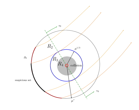
Figure 4. Geometry of the incoming curve near collisions, see (4).

   which is a graph over the configuration space so that incoming velocity satisfies certain quantitative estimates (see Prop. 3.1 for more details and Fig. 4). Inclusion (5) implies that $\mathcal{S}_{0}$ lies in the boundary of the local region $R_{1}^{c}=R_{2}\cup R_{3}$. Now we turn to a local analysis summarized on Fig. LABEL:lr.
   

2. (Transition zone) In this step we show that there exists a subsegment $\mathcal{S}^{\prime}_{0}\subset\mathcal{S}_{0}$ such that the push forward along the flow of $H_{\mu}$ becomes a segment

   $$\mathcal{S}_{1}\subset\partial R_{3}$$

   so that the shape of $\mathcal{S}_{1}$ and incoming velocity satisfy certain quantitative estimates (see Proposition 4.1 and Fig. LABEL:lr   for more details). In the region $R_{2}$, which is $\mu^{\frac{3}{20}}$-small we come with velocity $O(1)$ and show that linear approximation suffices, even though neither the Sun, nor Jupiter have dominant effect in this region.
   

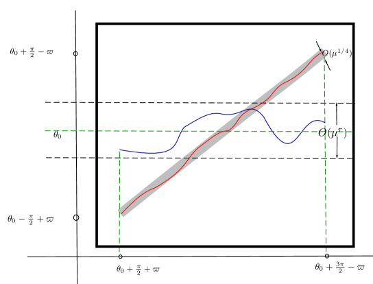
Figure 5. The Blue curve is the projection of $\mathcal{S}_{1}$ obtained in Proposition 4.1 onto the $(\mathrm{arg}(u),\mathrm{arg}(v))$ plane whereas the red curve is the projection onto the same plane of the curve $\Upsilon$ obtained in Corollary 5.3. We use the notation $\theta_{0}=\mathrm{arg}(v_{0})$.

3. (Levi-Civita region and the local manifold of collisions) In the region $R_{3}$, we can apply the Levi-Civita regularization and deduce a new system close to a linear hyperbolic system. We analyze the local manifold of collisions, denoted by $\Upsilon$ and show that $\mathcal{S}_{1}$ intersects $\Upsilon$. This implies the existence of collision orbits starting from $\mathcal{S}_{1}$, and, therefore, from $\mathfrak{S}$ (see Lemma 5.2 and Fig. 5).
   

Heuristic ideas in the proof: Here we describe main ideas of the proof:

• (From global to local) In order to control the long time evolution of $\mathfrak{S}$ we apply the following trick: Inside the local region $R_{2}\cup R_{3}$, we modify $H_{\mu}$ into $\widehat{H}_{\mu}$ by removing the singularity. This enables us to apply the KAM theorem. Thus we can pick up a segment $\mathfrak{S}$ on a suitable KAM torus $\mathcal{T}_{w}$ and show that the push forward along the flow of $H_{\mu}$ coincides with the flow of $\widehat{H}_{\mu}$, as long as it does not enter the collision region $R_{2}\cup R_{3}$. We also show that the final state of $\mathcal{S}_{0}$ is a graph over the configuration space with almost constant velocity component. More precisely, for any point in $\mathcal{S}_{0}$, the velocity is contained in a $O(\mu^{\frac{3}{20}})$ neighbourhood of a certain velocity $v_{0}$ (see Prop. 3.1 and Fig. 4 for more details).
  

• (Transition zone) We start with the curve $\mathcal{S}_{0}$, which has almost constant velocity. Then we flow the segment by the flow of $H_{\mu}$ using that it is close to linear. Controlling the evolution of the flow we get the desired estimate on the final state $\mathcal{S}_{1}$ of $\mathcal{S}_{0}$ (see Proposition 4.1 and Fig. LABEL:lr).
  

• (Levi-Civita region and local collision manifold) Once we have information about $\mathcal{S}_{1}$, the approximation by the linear hyperbolic system gives precise enough local information about the collisions manifold $\Upsilon$. This allows us to prove that $\mathcal{S}_{1}\bigcap\Upsilon\neq\emptyset$ by using the intermediate value theorem (see Lemma 5.2 and Fig. 5).
  

Organization of this paper: The paper is organized as follows. In Section 2, we introduce the Delaunay coordinates and discuss the integrable Hamiltonian (1) with $\mu=0$. In Section 3, we analyze the dynamics “far away” from collisions (Step 1 of the Scheme of the proof). We define the modified Hamiltonian $\widehat{H}_{\mu}$ and we apply the KAM theory. Then in Section 4 we analyze the dynamics in the transition zone (Step 2). In Section 5, we use the Levi–Civita regularization to analyze a small neighborhood of the collision (Step 4). This completes the proof of Theorem 1.3. Finally, in the Appendix we provide basic formulas for Delaunay coordinates.

Acknowledgments: The authors thank Alain Albouy, Alain Chenciner and Jacques Féjoz for helpful discussions and remarks on a preliminary version of the paper.

2. The collision set and density of collision orbits for $\mu=0$

We start by considering Hamiltonian (1) with $\mu=0$. This simplified model will give us the open set $\mathcal{V}$ where to look for (asymptotic) density of collisions. The analysis of this set was already done in [6]. Hamiltonian (1) with $\mu=0$ reads

(6) $$H_{0}(x,y)=\frac{|y|^{2}}{2}-x^{t}Jy-\frac{1}{|x|}.$$

If we perform the classical Delaunay transformation (see Appendix A) $\Psi(x,y)=(\ell,g,L,G),$ which is symplectic, to $H_{0}$ we obtain

(7) $$H_{0}(L,G)=-\frac{1}{2L^{2}}-G.$$

We use these coordinates to define the set $\mathcal{V}$ where collisions orbits are dense when $\mu=0$. We define also the eccentricity

(8) $$e=e(L,G)=\sqrt{1-\frac{G^{2}}{L^{2}}}.$$

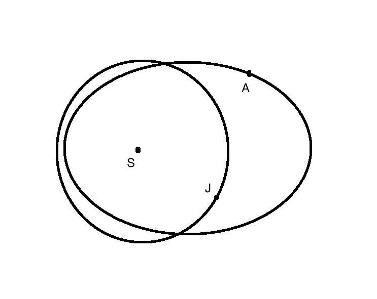
Figure 1. Elliptic and circular orbits of Asteroid and Jupiter resp. for $\mu=0$.

Lemma 2.1 ([6]).

Fix $J\in(-2\sqrt{2},3)$ and define the open set

$$\mathcal{V}=\left\{(\ell,g,L,G)\in\mathbb{T}^{2}\times(0,+\infty)\times(-L,0)\cup(0,L):\ \frac{G^{2}}{1+e}<1<\frac{G^{2}}{1-e}\right\}.$$

Then, the set

$$\mathcal{V}_{J}=\mathcal{V}\cap\{-2H_{0}=J\}$$

contains a dense subset whose orbits tend to collision.

Proof.

To prove this lemma, we express the collision set in Delaunay coordinates (see Appendix A). This expression is needed in Section 3. In polar coordinates the collisions are defined (when $\mu=0$) by

$$r=1,\quad\varphi=0.$$

By (47), this is equivalent to

(9) $$\begin{split}L^{2}(1-e\cos\mathfrak{u})&=1\\ \mathfrak{v}(\ell)+g&=0.\end{split}$$

To have solutions of the first equation, we impose

(10) $$\Big{|}\frac{L^{2}-1}{eL^{2}}\Big{|}<1,$$

which is equivalent to the condition

(11) $$\frac{G^{2}}{1+e}<1<\frac{G^{2}}{1-e},$$

imposed in the definition of $\mathcal{V}$. Assuming this condition, the first equation has two solutions in $[0,2\pi]$

$$\mathfrak{u}^{*}_{+}=\arccos{\frac{L^{2}-1}{eL^{2}}}\in(0,\pi),\quad\mathfrak{u}_{-}^{*}=2\pi-\arccos{\frac{L^{2}-1}{eL^{2}}}\in(\pi,2\pi).$$

Using $\ell=\mathfrak{u}-e\sin\mathfrak{u}$, we obtain $\ell_{\pm,0}^{*}(L,G)$. Finally, we can solve the second equation in (9) as $g_{\pm,0}^{*}(L,G)=-\mathfrak{v}(\ell^{*}_{\pm})$ to obtain the collision set as two graphs on the actions $(L,G)$,

(12) $$\begin{split}\ell&=\ell^{\pm,0}_{\mathrm{col}}(L,G)\\ g&=g^{\pm,0}_{\mathrm{col}}(L,G).\end{split}$$

Recall that $H_{0}(L,G)$ is completely integrable. For fixed $J\in(-2\sqrt{2},3)$,

$$\mathcal{V}\cap\{-2H_{0}(L,G)=J\}$$

is foliated by 2-dimensional tori defined by constant $(L,G)$ (see Fig. 2), whose dynamics is a rigid rotation with frequency vector $\omega=(\partial_{L}H_{0},-1)$. If $\partial_{L}H_{0}=L^{-3}\in\mathbb{R}\backslash\mathbb{Q}$, the orbit

$$\left\{\left.\varphi_{t}\left(\ell^{\pm,0}_{\mathrm{col}}(L,G),g^{\pm,0}_{\mathrm{col}}(L,G),L,\frac{J}{2}-\frac{1}{2L^{2}}\right)\ \right|\ t\in\mathbb{R}\right\}$$

is dense in the corresponding torus. Moreover, $\partial_{L}H_{0}={1}/{L^{3}}$ is a diffeomorphism of $(0,+\infty)$. Thus, for a dense set $L\in(0,+\infty)$, the frequency vector is non-resonant. These two facts lead to density of collisions lead to the existence of $\mathcal{V}$ of which collision solutions are dense. ∎

Lemma 2.1 does not only provide the open set $\mathcal{V}$ but also describes it in terms of the Delaunay coordinates. Let us explain the set $\mathcal{V}$ geometrically. We need to avoid the following:

• Degenerate ellipses with $e=1$: so we impose $G\neq 0$.

• Circles: so we impose $|G|<L$.

• Ellipses that do not intersect the orbit of the second primary (the unit circle) or are tangent to it. This is given by two conditions. The first one is (11). The second one is that the semimajor axis $L$ cannot be too small. This second condition is equivalent to take $H_{0}$ in the imposed range of energies $-2H_{0}=J\in(-2\sqrt{2},3)$.
  

The proof of Lemma 2.1 also provides a description of the collision manifold for $H_{0}$ in $\mathcal{V}\cap\{-2H_{0}(L,G)=J\}$. This manifold has two connected components in the energy level defined as

$$\mathcal{C}_{J}^{\pm}=\Big{\{}(\ell,g,L,G)\in\mathcal{V}\cap\{-2H_{0}(L,G)=J\}\Big{|}\ell=\ell_{\pm,0}^{*}(L,G),g=g_{\pm,0}^{*}(L,G)\Big{\}}$$

It can be easily seen that these manifolds intersect transversally each invariant torus $(L,G)=\mathrm{constant}$ in $\mathcal{V}\cap\{-2H_{0}(L,G)=J\}$.

Finally, let us point out that to prove Theorem 1.3 we cannot work with the full set $\mathcal{V}$ but in open sets whose closure is strictly contained in $\mathcal{V}$. Namely, the closer we are to the boundary of $\mathcal{U}$, the smaller we need to take $\mu$ to prove Theorem 1.3. To this end, we define the following open sets. Fix $\delta>0$ small. Recall that eccentricity $e=e(L,G)=\sqrt{1-\frac{G^{2}}{L^{2}}}$, see (8). Then, we define

$$\mathcal{V}_{\delta}\ \subset\ \overline{\mathcal{V}_{\delta}}\ \subset\ \mathcal{V},$$

where

(13) $$\mathcal{V}_{\delta}=\left\{(\ell,g,L,G)\right. \in\mathcal{V}:\ \ L\in(\delta,\delta^{-1}),$$

$$\left.\ \delta<|G|<L-\delta,\ \ \frac{G^{2}}{1+e(G,L)}+\delta<1<\frac{G^{2}}{1-e(G,L)}-\delta\right\}.$$

For $\mu>0$, one can analyze the collision set analogously as done in the proof of Lemma 2.1. One just needs to replace the equations (9) by

(14) $$\begin{split}L^{2}(1-e\cos\mathfrak{u})&=1-\mu\\ \mathfrak{v}(\ell)+g&=0.\end{split}$$

which have solutions in $\mathcal{V}_{\delta}$ for $\mu$ small enough and lead to a definition of the collision set as two graphs

(15) $$\begin{split}\ell&=\ell^{\pm,\mu}_{\mathrm{col}}(L,G)\\ g&=g^{\pm,\mu}_{\mathrm{col}}(L,G).\end{split}$$

Moreover, these graphs are non-degenerate in $\mathcal{V}_{\delta}$ as the associated Hessian has positive lower bounds (independent of $\mu$).

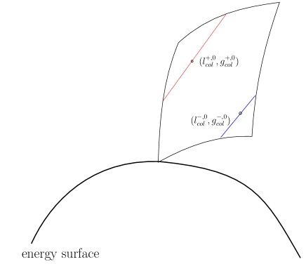
Figure 2. For $\mu=0$, the energy surface $\{-2H_{0}=J\}$ is foliated by punctured tori, where the punctures correspond to collisions.

3. The region $R_{1}$: dynamics far from collision

To study the region $R_{1}$, that is dynamics “far from collision”, we apply KAM Theory. To this end, we modify the Hamiltonian to avoid its blow up when approaching collision. We modify the Hamiltonian in polar coordinates and then we express the modified Hamiltonian in Delaunay variables.

The Hamiltonian (1) expressed in polar coordinates (45) is given by

(16) $$H_{\mu}(r,\varphi,R,G) = \frac{R^{2}}{2}+\frac{G^{2}}{2r^{2}}-G-\frac{\mu}{\sqrt{r^{2}+(1-\mu)^{2}-2(1-\mu)r\cos\varphi}}$$

$$-\frac{1-\mu}{\sqrt{r^{2}+\mu^{2}+2\mu r\cos\varphi}}$$

which can be written as

$$H_{\mu}(r,\varphi,R,G)=\frac{R^{2}}{2}+\frac{G^{2}}{2r^{2}}-G-\frac{1}{r}-\mu g_{1}(r,\varphi,\mu)-\mu g_{2}(r,\varphi,\mu),$$

where

$$\begin{split}g_{1}(r,\varphi,\mu)=&\frac{1}{\sqrt{r^{2}+(1-\mu)^{2}-2(1-\mu)r\cos\varphi}}\\ g_{2}(r,\varphi,\mu)=&\mu^{-1}\left(\frac{1}{\sqrt{r^{2}+\mu^{2}+2\mu r\cos\varphi}}-\frac{1}{r}\right).\end{split}$$

The term $g_{1}$ has a singularity at $\{(r,\varphi)=(1-\mu,0)\}$ and $g_{2}$ is analytic in the domains we are considering (which do not contain the position of the other primary). We modify $g_{1}$ by multiplying it by a $C^{\infty}$ smooth bump function. Consider $\Phi:\mathbb{R}\to\mathbb{R}$ so that

$$\Phi(z)=\left\{\begin{matrix}0\ \text{ if }\ |z|\leq 1\\ 1\ \text{ if }\ |z|\geq 2\end{matrix}\right.$$

Then, if we fix $\tau>0$, we define

$$\widehat{g}_{1}(r,\varphi,\mu)=\Phi\left(\mu^{-\tau}\sqrt{(r\cos\varphi-1+\mu)^{2}+r^{2}\sin^{2}\varphi}\right)\left({g}_{1}(r,\varphi,\mu)-4\mu^{-\tau}\right)+4\mu^{-\tau}.$$

with

$$\widehat{g}_{1}(r,\varphi,\mu)=\left\{\begin{split}g_{1}(r,\varphi,\mu),&\quad\text{for }|(r\cos\varphi-1-\mu,r\sin\varphi)|\geq 2\mu^{\tau}\\ 4\mu^{-\tau},&\quad\text{for }|(r\cos\varphi-1-\mu,r\sin\varphi)|\leq\mu^{\tau}.\\ \end{split}\right.$$

Later, in Section 3.2, we show that the optimal choice for $\tau$ is $\tau=3/20$.

Notice that $\|\widehat{g}_{1}\|_{C^{r}}\lesssim\mu^{-(r+1)\tau}$ for sufficiently small $\mu\ll 1$, and $\|g_{2}\|_{C^{r}}\lesssim 1$. In this section, we consider the modified Hamiltonian

(17) $$\widehat{H}_{\mu}(r,\varphi,R,G)=\frac{R^{2}}{2}+\frac{G^{2}}{2r^{2}}-G-\frac{1}{r}-\mu\widehat{g}_{1}(r,\varphi,\mu)+\mu g_{2}(r,\varphi,\mu),$$

and we express it in Delaunay coordinates by considering the transformation $\Psi_{2}(r,\varphi,R,G)=(\ell,g,L,G)$ introduced in (46). This change leads to an iso-energetic non-degenerate nearly integrable Hamiltonian

(18) $$\widehat{H}_{\mu}(\ell,g,L,G)=-\frac{1}{2L^{2}}-G+\mu\widehat{f}_{1}(\ell,g,L,G,\mu)-\mu f_{2}(\ell,g,L,G,\mu).$$

Fix $\delta>0$. Then, in the set $\mathcal{V}_{\delta}$ defined in (13), the functions $f_{1}$ and $f_{2}$ satisfy

$$\|\widehat{f}_{1}\|_{C^{r}}\leq C\mu^{-(r+1)\tau},\quad\|f_{2}\|_{C^{r}}\leq C$$

for some constant $C$ which depends on $\delta$ but is independent of $\mu$.

In polar coordinates, there are two disjoint subsets

(19) $$\mathcal{D}_{\mathrm{pol}}^{\pm}:=\Big{\{}(r,\varphi,R,G)\subset\Psi_{2}(\mathcal{V}_{\delta})\ \Big{|}\ \left|(r\cos\varphi-1+\mu,r\sin\varphi)\right|\leq\mu^{\tau}\Big{\}},$$

at each of the considered energy levels where the Hamiltonian $H_{\mu}$ in (16) is different from the modified $\widehat{H}_{\mu}$ in (17). They correspond to two disjoint intersections (see Fig. 1). Here the sign $\pm$ depends on the sign of the variable $R$.

The main result of this section is the following Proposition, where we take

$$\tau=\frac{3}{20}.$$

Note that we abuse notation and we refer to $\mathcal{V}_{\delta}$ independently of the coordinates we are using.

Proposition 3.1.

Fix $\delta>0$ and $\varpi>0$ small. Then there exists $\mu_{0}>0$ depending on $\delta$ and $\varpi$, such that the following holds for any $\mu\in(0,\mu_{0})$:

For any ${\mathbb{X}}\in\mathcal{V}_{\delta}$, there exists a $C^{1}$ curve $\mathfrak{S}\in\mathcal{V}_{\delta}$ of length $O(\mu^{\frac{3}{20}})$ satisfying

$$\mathrm{dist}(\mathfrak{S},\mathbb{X})\leq O(\mu^{\frac{1}{20}})$$

and a continuous function $T_{0}:\mathfrak{S}\to\mathbb{R}^{+}$ such that

$$\mathcal{S}_{0}=\left\{\phi_{H_{\mu}}(T_{0}(z),z):z\in\mathfrak{S}\right\}$$

satisfies either $\mathcal{S}_{0}\subset\partial\mathcal{D}_{\mathrm{pol}}^{+}$ or $\mathcal{S}_{0}\subset\partial\mathcal{D}_{\mathrm{pol}}^{-}$, where $\phi_{H_{\mu}}$ is the flow associated to the Hamiltonian $H_{\mu}$.

Moreover,

1. There exists a $C^{1}$ function $V$ satisfying such that $\mathcal{S}_{0}$ is a graph over $u$ as

   $$\mathcal{S}_{0}=\left\{(u,V(u))\ \left|\ \ \ u=\mu^{\frac{3}{20}}e^{is}\cdot\frac{v_{0}}{|v_{0}|},\quad s\in\left[\frac{\pi}{2}+\varpi,\frac{3\pi}{2}-\varpi\right]\right.\right\}.$$

   Moreover, there exists $v_{0}\in\mathbb{R}^{2}$ satisfying $|v_{0}|\geq C$ for certain $C>0$ independent of $\mu$ such that

   $$\max\,|V(u)-v_{0}|\leq O(\mu^{1/20}).$$

2. For all $z\in\mathfrak{S}$ and $t\in(0,T_{0}(z))$, $\phi_{\widehat{H}_{\mu}}(t,z)\not\in\mathcal{D}_{\mathrm{pol}}^{+}\cup\mathcal{D}_{\mathrm{pol}}^{-}$ and, therefore,

   $$\phi_{\widehat{H}_{\mu}}(t,z)=\phi_{H_{\mu}}(t,z),\quad\forall z\in\mathfrak{S}\text{ and }t\in(0,T_{0}(z)).$$

This proposition implies that any point in $\mathcal{V}_{\delta}$ has a curve $\mathfrak{S}$ in its $O(\mu^{\frac{1}{20}})$ neighborhood that hits “in a good way” a $O(\mu^{\frac{3}{20}})$ of the collision. To prove Theorem 1.3, it only remains to prove that the image curve $\mathcal{S}_{0}$ posesses a point whose orbit leads to collision. We prove this fact in two steps in Sections 4 and 5.

The rest of this section is devoted to prove Proposition 3.1.

Proof.

The proof has several steps. We first analyze the dynamics in the region $R_{1}$ in Delaunay coordinates, then translate into the Cartesian coordinates $(u,v)$.

3.1. Application of the KAM Theorem

First step is to apply KAM Theorem to get invariant tori for the Hamiltonian $\widehat{H}_{\mu}$. We are not aware of any KAM Theorem in the literature dealing with $C^{\infty}$ iso-energetically non-degenerate Hamiltonian systems. To overcome this problem, we reduce $\widehat{H}_{\mu}$ to a two dimensional Poincaré map and use Herman’s KAM Theorem [21].

Lemma 3.2.

Fix $r\geq 3$ and $\tau>0$ such that $1-(r+2)\tau>0$. Consider the Hamiltonian (18) and fix an energy level $\{\widehat{H}_{\mu}=h\},\ h\in(-3/2,\sqrt{2})$. Then, for $\mu$ small enough, the flow associated to (18) restricted to the level of energy induces a two dimensional exact symplectic Poincaré map $\mathcal{P}_{h,g_{0}}:\{g=g_{0}\}\to\{g=g_{0}\}$, $\mathcal{P}_{h,g_{0}}=\mathcal{P}_{h,g_{0}}(\ell,L)$. Moreover, $\mathcal{P}_{h,g_{0}}$ is of the form

$$\mathcal{P}_{h,g_{0}}:\begin{pmatrix}\ell\\ L\end{pmatrix}\to\begin{pmatrix}\ell-2\pi\omega(L)\\ L\end{pmatrix}+F\begin{pmatrix}\ell\\ L\end{pmatrix}$$

where

$$\omega(L)=\frac{1}{L^{3}}$$

and $F$ depends on both $h$ and $g_{0}$ and satisfies

$$\|F\|_{C^{r}}\leq C\mu^{1-(r+2)\tau}$$

for some $C>0$ independent of $\mu$.

We apply KAM Theory to the Poincaré map $\mathcal{P}_{h,g_{0}}$. Recall that a real number $\omega$ is called a constant type Diophantine number if there exists a constant $\gamma>0$ such that

(20) $$\left|\omega-\frac{p}{q}\right|\geq\frac{\gamma}{q^{2}}\qquad\text{ for all }p\in\mathbb{Z},\ \ q\in\mathbb{N}.$$

We denote by $B_{\gamma}$ the set of such numbers for a fixed $\gamma>0$. The set $B_{\gamma}$ has measure zero. Nevertheless, it has the following property.

Lemma 3.3.

Fix $\gamma\ll 1$. Then, the set $B_{\gamma}$ is $\gamma$-dense in $\mathbb{R}$

We prove this lemma in Appendix B.

Then we can apply the following KAM theorem.

Theorem 3.4 (M. Herman [21], Volume 1, Section 5.4 and 5.5).

Consider a $C^{r}$, $r\geq 4$, area preserving twist map

$$f_{\varepsilon}:[0,1]\times\mathbb{T}\rightarrow[0,1]\times\mathbb{T}\quad\text{of the form}\quad f_{\varepsilon}=f_{0}+\varepsilon f_{1},$$

where

$$f_{0}(\theta,I)=(\theta+A(I),I)$$

and $M_{0}^{-1}\geq A^{\prime}(I)\geq M_{0}>0$ for all $I\in\mathbb{R}$. Assume $\|f_{1}\|_{C^{r}}\lesssim 1$. Then, if $\varepsilon^{1/2}M_{0}^{-1}$ is small enough, for each $\omega$ from the set of constant type Diophantine numbers with $\gamma\sim\varepsilon^{1/2}$, the map $f_{\varepsilon}$ posesses an invariant torus $\mathcal{T}_{\omega}$ which is a graph of $C^{r-3}$ functions $U_{\omega}$ and the motion on $\mathcal{T}_{\omega}$ is $C^{r-3}$ conjugated to a rotation by $\omega$ with $\|U_{\omega}\|_{C^{r-3}}\lesssim\varepsilon^{1/2}$. These tori cover the whole annulus $O(\varepsilon^{1/2})$-densely.

Remark 3.5.

In [21] it is shown that this theorem is also valid under the weaker assumption that the map $f_{\varepsilon}$ is $C^{3+\beta}$ with any $\beta>0$ instead of $C^{4}$. This would slightly improve the density exponent in Theorem 1.3 as already pointed out in Remark 1.4 (see also the Remark 3.10 below). We stay with regularity $C^{4}$ to have simpler estimates.

This theorem can be applied to the Poincaré map obtained in Lemma 3.2. Moreover, these KAM tori have smooth dependence on $g_{0}$. Indeed, all Poincare maps $\mathcal{P}_{h,g_{0}}:\{g=g_{0}\}\to\{g=g_{0}\}$ with different $g_{0}$ are conjugate to each other.

Theorem 3.4 implies the existence of 2–dimensional tori $\mathcal{T}_{\omega}^{h}$ which are invariant by the flow of $\widehat{H}_{\mu}$ in (18) with energy $h=-J/2\in(-3/2,\sqrt{2})$. Note that we cannot identify the quasiperiodic frequency $\omega=(\omega_{\ell}^{h},\omega_{g}^{h})$ of the dynamics on $\mathcal{T}_{\omega}$, only that their ratio $\omega_{\ell}^{h}/\omega_{g}^{h}=-1/L_{0,\omega}^{3}$ is fixed (and Diophantine).

Corollary 3.6.

For each $\widehat{\omega}\in B_{\gamma}$ with $\gamma$ satisfying $\gamma\sim\varepsilon^{1/2}$ and any $h\in(-3/2,\sqrt{2})$ fixed, there is a KAM torus $\mathcal{T}^{h}_{\omega}$, which is given by

$$\mathcal{T}_{\omega}^{h}=\{(\ell,g,L_{\omega,\mu}^{h}(\ell,g),G_{\omega,\mu}^{h}(\ell,g))\ |\ (\ell,g)\in\mathbb{T}^{2}\}$$

where $\omega_{2}/\omega_{1}=\widehat{\omega}$ and $(L_{\omega,\mu}^{h},G_{\omega,\mu}^{h})$ is a $C^{r-3}$ graph satisfying

(21) $$\|L_{\omega,\mu}^{h}-L_{\omega,0}\|_{C^{r-3}}\lesssim\varepsilon^{1/2},\quad\|G_{\omega,\mu}^{h}-G_{\omega,0}\|_{C^{r-3}}\lesssim\varepsilon^{1/2}$$

where $\varepsilon=\mu^{1-6\tau}$,

$$\widehat{\omega}=\frac{1}{L_{0,\omega}^{3}},\quad h=-\frac{1}{2L_{0,\omega}^{2}}-G_{0,\omega}.$$

Moreover, $\bigcup_{\omega\in B^{\gamma}}\mathcal{T}_{\omega}^{h}$ is $O(\gamma)$-dense in $\mathcal{V}_{\delta}$.

This corollary is a direct application of Theorem 3.4. The frequency in this setting is given by $\omega(L)={1}/L^{3}$ and, thus

$$\left|\omega^{\prime}(L)\right|=\frac{3}{L^{4}}$$

has a lower bound independent of $\mu$ (but depending on $\delta$) in $\mathcal{V}_{\delta}$. Since the lower is regularity, the better are estimates for $\varepsilon$ we choose $r=4$. To simplify notation, we omit the superindex $h$. Note that the density of the KAM tori is due to the $\gamma$-density of $B_{\gamma}$, the relation between $\widehat{\omega}$ and $L$ and (21).

Remark 3.7.

Note that one can apply Theorem 3.4 with any $\gamma\gtrsim\sqrt{\varepsilon}$ at the expense of obtaining a worse density of invariant tori. In Section 3.2, we choose $\gamma$ to optimize density for the collision orbits.

3.2. The segment density argument in Delaunay coordinates

We use the KAM Theorem to obtain the segment density estimates stated in Proposition 3.1. We first obtain this density result in Delaunay coordinates. Taking into account that the change from Delaunay to the Cartesian coordinates $(u,v)$ is a diffeomorphism with uniform bounds independent of $\mu$, this will lead to the density estimates in Proposition 3.1.

For $\mu=0$ Lemma 2.1 describes the collision set in Delaunay coordinates as (two) graphs over the actions $(L,G)$ (see (12)). By the implicit function theorem the same holds for small $\mu>0$ (see (14)). Since the KAM tori obtained in Corollary 3.6 are graphs over $(\ell,g)$ and “almost horizontal” (see (21)), the intersection between each of these KAM tori $\mathcal{T}$ and the collision set consist of two points $(\ell_{\mathrm{col}}^{\pm,\mu},g_{\mathrm{col}}^{\pm,\mu},L(\ell_{\mathrm{col}}^{\pm,\mu},g_{\mathrm{col}}^{\pm,\mu}),G(\ell_{\mathrm{col}}^{\pm,\mu},g_{\mathrm{col}}^{\pm,\mu}))$. Denote the restriction of the collision neighborhoods $\mathcal{D}^{\pm}_{\mathrm{pol}}$ to these cylinders by $\mathcal{D}^{\pm}$. Since the coordinate change from the polar coordinates to Delaunay is a diffeomorphism there are constants $C>C^{\prime}>0$ independent of $\mu$ such that

(22) $$\partial\mathcal{D}^{\pm}\subset\left\{C^{\prime}\mu^{\tau}\leq|(\ell-\ell^{\pm,\mu}_{\mathrm{col}},g-g_{\mathrm{col}}^{\pm,\mu})|\leq C\mu^{\tau}\right\}.$$

For any of the tori $\mathcal{T}$ obtained in Corollary 3.6 we consider their graph parameterization

$$\mathcal{T}=\{(\ell,g,L_{\omega,\mu}^{h}(\ell,g),G_{\omega,\mu}^{h}(\ell,g))|(\ell,g)\in\mathbb{T}^{2}\}$$

and we define the balls

(23) $$\mathcal{B}_{\mathcal{T}}^{\pm}=\mathcal{T}\cap\left\{|(\ell-\ell^{\pm,\mu}_{\mathrm{col}},g-g_{\mathrm{col}}^{\pm,\mu})|\leq C\mu^{\tau}\right\}.$$

These balls can be viewed on Fig. 2 as neighborhoods of marked collision points in each torus. The main result of this section is the following lemma.

Lemma 3.8.

Fix $\delta>0$ and $\varpi>0$ small. Then, there exists $\mu_{0}>0$ depending on $\delta$ and $\varpi$, such that the following holds for any $\mu\in(0,\mu_{0})$:

For any ${\mathbb{X}}\in\mathcal{V}_{\delta}$, there exists a invariant torus $\mathcal{T}$ obtained in Corollary 3.6 and a $C^{1}$ curve $\mathfrak{S}\subset\mathcal{T}$ of length $O(\mu^{\frac{3}{20}})$ satisfying $\mathrm{dist}(\mathfrak{S},\mathbb{X})\leq O(\mu^{\frac{1}{20}})$ and a continuous function $T_{0}:\mathfrak{S}\to\mathbb{R}^{+}$ such that

$$\mathcal{S}_{0}=\left\{\phi_{H_{\mu}}(T_{0}(z),z):z\in\mathfrak{S}\right\}$$

satisfies either $\mathcal{S}_{0}\in\partial\mathcal{B}_{\mathcal{T}}^{+}$ or $\mathcal{S}_{0}\in\partial\mathcal{B}_{\mathcal{T}}^{-}$. In addition,

1. The set $\mathcal{S}_{0}$ is a graph over $(\ell,g)$ and satisfies either

   $$\begin{split}\mathcal{S}_{0}=\Big{\{}(\ell,g,L_{\omega,\mu}^{h}(\ell,g),G_{\omega,\mu}^{h}(\ell,g))\Big{|}&(\ell,g)=(\ell^{+,\mu}_{\mathrm{col}},g^{+,\mu}_{\mathrm{col}})+\mu^{\frac{3}{20}}e^{is}\cdot\frac{\omega}{|\omega|},\\ &s\in\left[\frac{\pi}{2}+\varpi,\frac{3\pi}{2}-\varpi\right]\Big{\}}.\end{split}$$

   or the same for the collision $(\ell^{-,\mu}_{\mathrm{col}},g^{-,\mu}_{\mathrm{col}})$.

2. For all $z\in\mathfrak{S}$ and $t\in(0,T_{0}(z))$, $\phi_{\widehat{H}_{\mu}}(t,z)\not\in\mathcal{B}_{\mathcal{T}}^{+}\cup\mathcal{B}_{\mathcal{T}}^{-}$ and therefore

   $$\phi_{\widehat{H}_{\mu}}(t,z)=\phi_{H_{\mu}}(t,z),\quad\forall z\in\mathfrak{S}\ \text{ and }\ t\in(0,T_{0}(z)).$$

We devote the rest of the section to prove this lemma. Since the segments $\mathfrak{S}$ considered are contained in the KAM tori from Corollary 3.6, we will use the density of tori to ensure that any point in $\mathcal{V}_{\delta}$ has one of those segments nearby. Thus, we need to ensure that

• By adjusting $\gamma$ in Corollary 3.6: the KAM tori are dense enough (see Remark 3.7).

• There are segments whose future evolution “spreads densely enough” on these tori.

Item 2 requires strong (Diophantine) properties on the frequency of the torus. The stronger the conditions we impose on the frequency, the better the spreading at expense of having fewer tori. This would give worse density in item 1. Thus, we need to obtain a balance between the density of tori in the phase space and the good spreading of orbits in the chosen tori.

Fix one torus $\mathcal{T}$ from Corollary 3.6 and consider the associated balls $\mathcal{B}_{\mathcal{T}}^{\pm}$ given by (23). To obtain the density statement, we first prove it for points belonging to the torus $\mathcal{T}$. Then due to sufficient density of KAM tori, we deduce Lemma 3.8 .

We want to show that any point $z\in\mathcal{T}$ has a segment $\mathfrak{S}\subset\mathcal{T}$ in its $O(\mu^{\frac{1}{20}})$ neighborhood which, under the flow of Hamiltonian (1) (in Delaunay coordinates), hits “in a good way” either $\partial\mathcal{B}_{\mathcal{T}}^{-}$ or $\partial\mathcal{B}_{\mathcal{T}}^{+}$, namely, covering a large enough part of the boundary of the balls and incoming velocity being almost constant (see Fig. 4). Note that we apply KAM to the Hamiltonian (18) instead of the original one (1). Since the Hamiltonian coincide only away from the union $\mathcal{B}_{\mathcal{T}}^{-}\cup\mathcal{B}_{\mathcal{T}}^{+}$, we need to make sure that the evolution of $\mathfrak{S}$ does not intersect this union before hitting it “in a good way”.

To start, assume that $\mathcal{T}$ has only one collision instead. Making a translation, we can assume that it is located at $(\ell,g)=(0,0)$. Later, we adapt the construction to deal with tori having two collisions.

One collision model case:   Since $\mathcal{T}$ is a graph on $(\ell,g)$, we analyze the density in the projection onto the base. By Theorem 3.4, the torus and its dynamics are $\varepsilon^{1/2}=\mu^{(1-6\tau)/2}$-close to the unperturbed one. Moreover, after a $\varepsilon^{1/2}$-close to the identity transformation, the base dynamics is a rigid rotation. Somewhat abusing notation we still denote transformed variables $(\ell,g)$. We analyze the density on the section $\{g=0\}$. Since the dynamics is a rigid rotation, the density in the section implies the density in the whole torus.

We flow backward the collision and analyze the intersections of the orbits with $\{g=0\}$. By a change of time, the orbits on the projection are just

(24) $$(\ell(t),g(t))=(\ell^{0}+\omega t,g^{0}+t),$$

where $\omega\in B_{\gamma}$, defined in (20), with $\gamma\gtrsim\sqrt{\varepsilon}$. The intersections of the backward orbit starting at the collision $(0,0)$ with $\{g=0\}$ are given by $\|q\omega\|$, where

(25) $$\|\alpha\|=\min_{p\in\mathbb{Z}}|\alpha-p|.$$

Fix $C>0$. We study this orbit until it hits again a $C\mu^{\tau}$ neighborhood of the collision. Thus, we consider $q=-1,\ldots,-q^{*}$ where $q^{*}+1\in\mathbb{N}$ is the smallest solution to

$$\|(q^{*}+1)\omega\|\leq 4C\mu^{\tau}.$$

Assume that the (ratio of) frequencies of the torus $\mathcal{T}$ is in $B_{\gamma}$ (with $\gamma$ to be specified later). Then, we obtain that

(26) $$|q^{*}|\geq\frac{1}{4C}\gamma\mu^{-\tau}-1.$$

We need to study the density of $-q\omega\,\,(\mathrm{mod}\,1)$ with $q=-1,\ldots,-q^{*}$. We apply the following non-homogeneous Dirichlet Theorem (see [11]), where we use the notation (25).

Theorem 3.9.

Let $L(x)$, $x=(x_{1},\ldots,x_{n})$ be a linear form and fix $A,X>0$. Suppose that there does not exist any $x\in\mathbb{Z}^{n}\setminus 0$ such that

$$\|L(x)\|\leq A\,\,\,\text{ and }\,\,\,|x_{i}|\leq X.$$

Then, for any $a\in\mathbb{R}$, the equations

$$\|L(x)-a\|\leq A_{1}\,\,\,\text{ and }\,\,\,|x_{i}|\leq X_{1}.$$

have an integer solution, where

$$A_{1}=\frac{1}{2}(h+1)A,\ \ \ X_{1}=\frac{1}{2}(h+1)X\,\,\textup{ and }\,\,h=X^{-n}A^{-1}.$$

We use this theorem to show that the iterates $-q\omega\,\,(\mathrm{mod}\,1)$ are $\gamma$-dense.

Since the frequency $\omega$ is in $B_{\gamma}$, the equation $\|q\omega\|<\gamma X^{-1}$ has no solution for $|q|\leq X$ and any $X>0$. Therefore, Theorem 3.9 implies that for any $\omega\in\mathbb{R}/\mathbb{Z}$ there exists $q$ satisfying

$$\|q\omega-\alpha\|\leq\frac{1}{X}\quad\text{ and }\quad|q|\leq X\gamma^{-1}$$

We take $q^{*}=[X\gamma^{-1}]$. Since we need $\gamma$-density, $X=\gamma^{-1}$. Then, using also (26), we obtain the following condition

$$\gamma^{-2}=|q^{*}|\geq\frac{1}{4C}\gamma\mu^{-\tau}-1\geq\frac{1}{5C}\gamma\mu^{-\tau}.$$

Moreover, to apply Corollary 3.6, one needs

$$\gamma\gtrsim\mu^{\frac{1-6\tau}{2}}.$$

Thus, one can take, in particular $\gamma\geq(5C)^{\frac{1}{3}}\mu^{\frac{1-6\tau}{2}}$. Then, it is easy to check that taking

$$\tau=\frac{3}{20},\qquad\gamma=C\mu^{\frac{1}{20}}.$$

for $C>1$ large enough independent of $\mu$, the two inequalities are satisfied. Moreover, this choice of $\gamma$, optimizes the density of both KAM tori and the spreading of orbits in these tori.

Remark 3.10.

If one considers regularity $C^{3+\beta}$ with $\beta>0$ small instead of $C^{4}$, as explained in Remark 3.5, one can proceed analogously. One would obtain then

$$\tau=\frac{3}{17+3\beta},\qquad\gamma=C\mu^{\frac{1}{17+3\beta}}.$$

This would lead to the improved density pointed out in Remark 1.4.

Two collisions in each torus:   The reasoning above has the simplifying assumption that each torus has only one collision instead of two. Now we incorporate the second collision. Note that the only problem of including the other collision is that the considered backward orbit departing from collision 1 located at $(0,0)$ may have intersected the $4C\mu^{\tau}$-neighborhood of the other collision, where the two flows $\phi_{\widehat{H}_{\mu}}(t,z)$ and $\phi_{H_{\mu}}(t,z)$ differ, before reaching the final time $t=-q^{*}$. We prove that the backward orbit until time $-q^{*}$ from one collision may intersect the $4C\mu^{\tau}$-neighborhood of the other collision, but this cannot happen for the $(-q^{*})$-time backward orbits of the two collisions, just for one of them.

Assume that the collisions are located at $(0,0)$ and $(\ell^{\prime},g^{\prime})$. Call $(\ell^{\prime\prime},0)$ the first intersection between $g=0$ and the backward orbit of the point $(\ell^{\prime},g^{\prime})$ under the flow (24) (see Figure 2). The time to go from $(\ell^{\prime},g^{\prime})$ to $(\ell^{\prime\prime},0)$ is independent of $\mu$ and, therefore, studying returns to the $1$-dimensional section suffices. Assume that both the $(-q^{*})$-backward orbit of $(0,0)$ hits a $4C\mu^{\tau}$ neighborhood of $(\ell^{\prime\prime},0)$ and the $(-q^{*})$-backward orbit of $(\ell^{\prime\prime},0)$ hits a $4C\mu^{\tau}$ neighborhood of $(0,0)$. That is, there exist $0\leq q_{1},q_{2}\leq q^{*}$ such that

$$\begin{split}\|q_{1}\omega-\ell^{\prime\prime}\|&<4C\mu^{\tau}\\ \|q_{2}\omega+\ell^{\prime\prime}\|&<4C\mu^{\tau}.\end{split}$$

Using the Diophantine condition

$$\frac{\gamma}{|q_{1}+q_{2}+2|}\leq\|(q_{1}+q_{2}+2)\omega\|\leq\|(q_{1}+1)\omega-\ell^{\prime\prime}\|+\|(q_{2}+1)\omega+\ell^{\prime\prime}\|<8C\mu^{\tau}.$$

Therefore, $q_{1}+q_{2}>8C\gamma\mu^{-\tau}-2$ which, by (26), implies that either $q_{1}$ or $q_{2}$ satisfies $q_{i}>4C\gamma\mu^{-\tau}-1$. This contradicts $q_{i}\leq q^{*}$.

Thus, the $(-q^{*})$-backward orbit under the flow $\phi_{H_{\mu}}$ of one of the two collisions covers the torus $\mu^{\frac{1}{20}}$–densely. Equivalently, for any point $(\ell_{0},g_{0})$ in the torus, there exists a point $(\ell^{*},g^{*})$ which is $\mu^{\frac{1}{20}}$-close to a trajectory of the flow $\phi_{H_{\mu}}$ hitting either $\partial\mathcal{B}_{\mathcal{T}}^{-}$ or $\partial\mathcal{B}_{\mathcal{T}}^{+}$. Now, since the invariant tori are $\gamma\sim\mu^{\frac{1}{20}}$ dense in $\mathcal{V}_{\delta}$ by Corollary 3.6, we have that the $\mu^{\frac{1}{20}}$ neighborhood of any point in $\mathcal{V}_{\delta}$ contains a point whose orbit reaches either $\partial\mathcal{B}_{\mathcal{T}}^{-}$ or $\partial\mathcal{B}_{\mathcal{T}}^{+}$.

We do not want just one orbit to hit $\partial\mathcal{B}_{\mathcal{T}}^{\pm}$ but we want a whole segment of length $\sim\mu^{\frac{3}{20}}$ to hit as stated in Item 1 of Lemma 3.8. Since we have considered coordinates such that the dynamics on $\mathcal{T}$ is a rigid rotation, one can see that the orbit of any point $C\mu^{\tau}$-close to $(\ell^{*},g^{*})$ does not hit $\mathcal{B}_{\mathcal{T}}^{+}$ for time $q^{*}+O(1)$ either. Therefore, $\mu^{\frac{1}{20}}$-close to any point one can construct a segment which hits $\partial\mathcal{B}_{\mathcal{T}}^{+}$ as stated in Item 1 of Lemma 3.8.

The considered coordinates are different but $\varepsilon^{1/2}$-close to the original $(\ell,g)$ (recall that abusing notation we have kept the same notation for both systems of coordinates). Nevertheless, all the statements proven are coordinate free and, therefore, are still valid in the original $(\ell,g)$ coordinates.

Moreover, the localization in actions is a direct consequence from the graph property in Corollary 3.6. Item 2 is a direct consequence of the fact that the constructed orbits do not intersect $\mathcal{B}_{\mathcal{T}}^{\pm}$ until they hit its boundary at time $q^{*}+O(1)$. This completes the proof of Lemma 3.8.

3.3. Back to Cartesian coordinates: proof of Proposition 3.1

To deduce Proposition 3.1 from Lemma 3.8 it only remains to change coordinates to $(u,v)$. Note that the only statement which is not coordinate free in Lemma 3.8 is the graph property and localization in the variable $v$ in Item 1. To this end we need to analyze the change of coordinates $(\ell,g)\to u$ in a neighborhood of the collisions (note that the graph property is only stated in these neighborhoods).

Using the Delaunay transformation and the graph property obtained in Lemma 3.8, the segment $\mathcal{S}$ expressed in cartesian coordinates can be parameterized as

$$\begin{split}u\equiv u(\ell,g,L,G)=u(\ell,g,L(\ell,g),G(\ell,g)),\ v\equiv v(\ell,g,L,G)=v(\ell,g,L(\ell,g),G(\ell,g)).\end{split}$$

It only remains to show that we can invert the first row to express $(\ell,g)$ as a function of $u$. As a first step, we can express $(\ell,g)$ in terms of the polar coordinates $(r,\varphi)$. Using the definition of Delaunay coordinates, one can easily check that

$$\left|\frac{\partial(\ell,g)}{\partial(r,\varphi)}\right|=\left|\begin{pmatrix}\partial_{r}\ell&0\\ \partial_{r}g&\partial_{\varphi}g\end{pmatrix}\right|=\left|\partial_{r}\ell\cdot\partial_{\varphi}g\right|=\left|\frac{1-e\cos u}{L^{2}e\sin u}\right|.$$

The location of the collisions in Delaunay coordinates has been given in (14). This implies that in a $\mu^{\tau}$–neighborhood of the collisions

$$1-e\cos u=\frac{1}{L^{2}}+O(\mu^{\tau})\neq 0$$

Moreover, by condition (10), $|\cos u|<1-\delta^{\prime}$ for some $\delta^{\prime}>0$ independent of $\mu$ and depending only on the parameter $\delta$ introduced in (13). This implies that $|\sin u|\geq\delta^{\prime\prime}$ for some $\delta^{\prime\prime}>0$ only depending on $\delta^{\prime}$. This implies that the change $(r,\varphi)\to(\ell,g)$ is well defined and a diffeomorphism in a $\mu^{\tau}$–neighborhood of the collisions. Since $(r,\varphi)\to u$ is a diffeomorphism, this gives the graph property stated in Proposition 3.1.

Now, we need to prove the localization of the velocity $v$. To this end, it suffices to define the velocity $v_{0}$ as

$$v_{0}=v\left(\ell_{\mathrm{col}}^{\pm,\mu},g_{\mathrm{col}}^{\pm,\mu},L_{\omega,\mu}(\ell_{\mathrm{col}}^{\pm,\mu},g_{\mathrm{col}}^{\pm,\mu}),G_{\omega,\mu}(\ell_{\mathrm{col}}^{\pm,\mu},g_{\mathrm{col}}^{\pm,\mu})\right).$$

That is, the velocity $v$ evaluated on the (removed) collision point at the torus $\mathcal{T}$. Here the choice of $+$ or $-$ depends on the neighborhood of what collision the segment $\mathcal{S}_{0}$ has hit. Using the smoothness of the torus, the estimate (21) and estimates on the changes of coordinates just mentioned, one can obtain the localization in Item 1 of Proposition 3.1.

Finally, let us mention that Lemma 3.8 considers $\mathcal{S}_{0}\subset\partial\mathcal{B}_{\mathcal{T}}^{\pm}$ (see (23)). On the contrary, Propostion 3.1 considers $\mathcal{S}_{0}$ at $\partial\mathcal{D}_{\mathrm{pol}}^{\pm}$ (see (19)). These balls do not coincide since are expressed in different variables. Nevertheless, the boundaries are very close as stated in (22). Since the flow is close to integrable in the annulus in (22), one can flow $\mathcal{S}_{0}$ from $\partial\mathcal{B}_{\mathcal{T}}^{\pm}$ to $\partial\mathcal{D}_{\mathrm{pol}}^{\pm}$ keeping all the stated properties. ∎

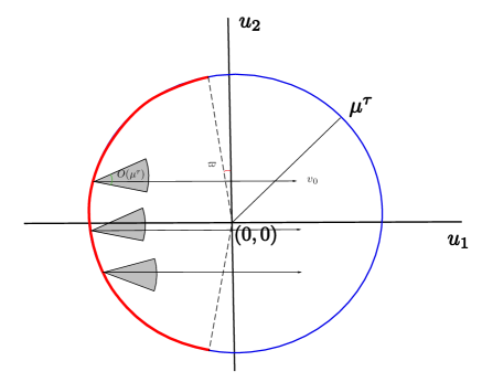
Figure 3. Projection of $\mathcal{S}_{0}$ onto the configuration space along with incoming velocity, which must belong to the grey cones.

4. The transition region $R_{2}$

In this section, we analyze the evolution of the segment $\mathcal{S}_{0}$ in the Transition Region (see (4)). More precisely, the goal is to prove that the evolution under the flow of $H_{\mu}$ of a subset of $\mathcal{S}_{0}$ reaches the inner boundary of the annulus $R_{2}$ (see (4)) and to obtain properties of this image set (see Fig. LABEL:lr).

To this end, we take $\rho>0$ and we consider a section $\Gamma_{1}$ transversal to the flow

$$\begin{split}\Gamma_{1}=&\Big{\{}\xi e^{i\pi/2}\frac{v_{0}}{|v_{0}|}\in\mathbb{R}^{2}\Big{|}\xi\in[-\mu^{\tau},-\rho\mu^{1/2}\sec\frac{\varpi}{2}]\cup[\rho\mu^{1/2}\sec\frac{\varpi}{2},\mu^{\tau}]\ \Big{\}}\bigcup\\ &\Big{\{}\lambda\rho\mu^{1/2}e^{i(\frac{\varpi}{2}+\frac{\pi}{2})}\frac{v_{0}}{|v_{0}|}+(1-\lambda)\rho\mu^{1/2}\sec\frac{\varpi}{2}e^{i\pi/2}\frac{v_{0}}{|v_{0}|}\Big{|}\ \lambda\in[0,1]\Big{\}}\ \bigcup\,\Gamma_{1,\varpi}\end{split}$$

where

(27) $$\Gamma_{1,\varpi}:=\left\{\rho\mu^{1/2}e^{i\theta}\cdot\frac{v_{0}}{|v_{0}|}\left|\theta\in\left[\frac{\pi}{2}+\frac{\varpi}{2},\frac{3\pi}{2}-\frac{\varpi}{2}\right]\right.\right\},$$

(see Fig. LABEL:lr ). The main result of this section is the following.

Proposition 4.1.

Consider the curve $\mathcal{S}_{0}$ defined in Proposition 3.1. Then, for $\rho>0$ large enough and $\mu>0$ small enough, there exists a subset $\mathcal{S}^{\prime}_{0}\subset\mathcal{S}_{0}$ such that for all $P\in\mathcal{S}^{\prime}_{0}$ there exists a time $T_{1}(P)>0$ continuous in $P\in\mathcal{S}^{\prime}_{0}$ such that

$$\Gamma_{1,\varpi}\subset\pi_{u}\Big{\{}\phi_{H_{\mu}}(T_{1}(P),P):P\in\mathcal{S}^{\prime}_{0}\Big{\}}\subset\Gamma_{1},$$

where $\phi_{H_{\mu}}(t,\cdot)$ is the flow associated to the Hamiltonian (1).

Moreover, if we denote by

$$\mathcal{S}_{1}:=\Big{\{}\phi_{H_{\mu}}(T_{1}(P),P)\Big{|}\ P\in\mathcal{S}^{\prime}_{0}\Big{\}},$$

the following properties hold

• $\mathcal{S}_{1}$ is a $C^{0}$ curve.

• For all $P\in\mathcal{S}_{1}$ , $\|\pi_{v}P-v_{0}\|\leq O(\mu^{\tau/3})$.

• For all $P\in\mathcal{S}_{1}$, $T_{1}(P)\lesssim\mu^{\tau}$.

To prove Proposition 4.1 we first consider a first order of the equations associated to Hamiltonian $H_{\mu}$ in (1). Taking into account that in the region $R_{2}$ we have that $|u|\leq\mu^{\tau}$ (see (4)), we define the Hamiltonian

(28) $$H_{\mathrm{lin}}(u,v)=\frac{|v|^{2}}{2}-u^{t}Jv,$$

which will be a “good first order” of $H_{\mu}$ and whose equations are linear,

$$\begin{split}\dot{u}_{1}&=v_{1}+u_{2}\\ \dot{u}_{2}&=v_{2}-u_{1}\\ \dot{v}_{1}&=v_{2}\\ \dot{v}_{2}&=-v_{1}.\end{split}$$

Lemma 4.2.

Consider the curve $\mathcal{S}_{0}$ defined in Proposition 3.1. Then, there exists a subset $\mathcal{S}^{\mathrm{lin}}_{0}\subset\mathcal{S}_{0}$ such that for all $P\in\mathcal{S}^{\mathrm{lin}}_{0}$ there exists a time $T_{\mathrm{lin}}(P)>0$ continuous in $P\in\mathcal{S}^{\mathrm{lin}}_{0}$ such that

(29) $$\Gamma_{1,\varpi}\subset\pi_{u}\Big{\{}\phi_{H_{\mathrm{lin}}}({T_{\mathrm{lin}}(P)},P):P\in\mathcal{S}^{\mathrm{lin}}_{0}\Big{\}}\subset\Gamma_{1},$$

where $\Gamma_{1,\varpi}$ has been defined in (27) and $\phi_{H_{\mathrm{lin}}}(t,\cdot)$ is the flow associated to Hamiltonian (28). Moreover, if we define

$$\mathcal{S}^{\mathrm{lin}}_{1}=\Big{\{}\phi_{H_{\mathrm{lin}}}({T_{\mathrm{lin}}(P)},P)\Big{|}P\in\mathcal{S}^{\mathrm{lin}}_{0}\Big{\}},$$

the following properties hold

• $\mathcal{S}^{\mathrm{lin}}_{1}$ is a $C^{0}$ curve.

• For all $P\in\mathcal{S}^{\mathrm{lin}}_{1}$ , $\|\pi_{v}P-v_{0}\|\leq O(\mu^{\tau/3})$.

• For all $P\in\mathcal{S}^{\mathrm{lin}}_{1}$, $T_{\mathrm{lin}}(P)\leq O(\mu^{\tau})$.

Proof.

The proof of this lemma is straightforward taking into account that $|u|\lesssim\mu^{\tau}$ in $R_{2}$, that the trajectories associated to the Hamiltonian in (28) are explicit and given by

$$\begin{split}\begin{pmatrix}u_{1}\\ u_{2}\end{pmatrix}&=\begin{pmatrix}\cos t&\sin t\\ -\sin t&\cos t\end{pmatrix}\begin{pmatrix}u_{1}^{0}\\ u^{0}_{2}\end{pmatrix}+t\begin{pmatrix}\cos t&\sin t\\ -\sin t&\cos t\end{pmatrix}\begin{pmatrix}v_{1}^{0}\\ v^{0}_{2}\end{pmatrix}\\ \begin{pmatrix}v_{1}\\ v_{2}\end{pmatrix}&=\begin{pmatrix}\cos t&\sin t\\ -\sin t&\cos t\end{pmatrix}\begin{pmatrix}v_{1}^{0}\\ v^{0}_{2}\end{pmatrix}\end{split}$$

and the fact that $(v_{1}^{0},v^{0}_{2})$ has a lower bound independent of $\mu$. ∎

Once Lemma 4.2 has given the behavior in Region $R_{2}$ of the flow associated to the Hamiltonian (28), now we compare its dynamics to those of $H_{\mu}$ in (1).

Lemma 4.3.

Take $\rho>0$ large enough and $\mu>0$ small enough. Then, for all $P\in\mathcal{S}_{0}$, there exists $T_{1}(P)>0$ continuous in $P$ satisfying

(30) $$|T_{1}(P)-T_{\mathrm{lin}}(P)|\lesssim\rho^{-1}\mu^{2\tau}$$

such that $\pi_{u}\phi_{H_{\mu}}(t,P)\in\mathrm{Int}(R_{2})$ for all $t\in(0,T_{1}(P))$, $\pi_{u}\phi_{H_{\mu}}(T_{1}(P),P)\in\Gamma^{1}$ with

(31) $$\left\|\pi_{v}\phi_{H_{\mu}}(T_{1}(P),P)-\pi_{v}\,\phi_{H_{\mathrm{lin}}}(T_{\mathrm{lin}}(P),P)\right\|\lesssim\rho^{-1}\mu^{2\tau}.$$

Proof.

The region $R_{2}$ satisfies $|u|\leq\mu^{\tau}$. Therefore, the equation associated to Hamiltonian $H_{\mu}$ in (1) satisfies

$$\begin{split}\dot{u}_{1}&=v_{1}+u_{2}\\ \dot{u}_{2}&=v_{2}-u_{1}\\ \dot{v}_{1}&=v_{2}+O\left(\rho^{-1}+\mu\right)\\ \dot{v}_{2}&=-v_{1}+O\left(\rho^{-1}+\mu\right).\end{split}$$

Since $\rho$ is taken such that $\rho^{-1}\gg\mu$; we have that this equation is $O(\rho^{-1})$–close to the equation of $H_{\mathrm{lin}}$ (see (28)).

Consider the trajectory $(u(t),v(t))$ of $(u^{0},v^{0})\in\mathcal{S}_{0}$ under the flow of $H_{\mu}$. Then, applying variation of constants formula, as long as the trajectory remains in $R_{2}$, we have

$$\begin{split}\begin{pmatrix}u_{1}\\ u_{2}\end{pmatrix}&=\begin{pmatrix}\cos t&\sin t\\ -\sin t&\cos t\end{pmatrix}\begin{pmatrix}u_{1}^{0}\\ u^{0}_{2}\end{pmatrix}+t\begin{pmatrix}\cos t&\sin t\\ -\sin t&\cos t\end{pmatrix}\begin{pmatrix}v_{1}^{0}\\ v^{0}_{2}\end{pmatrix}+O\left(\rho^{-1}t^{2}\right)\\ \begin{pmatrix}v_{1}\\ v_{2}\end{pmatrix}&=\begin{pmatrix}\cos t&\sin t\\ -\sin t&\cos t\end{pmatrix}\begin{pmatrix}v_{1}^{0}\\ v^{0}_{2}\end{pmatrix}+O\left(\rho^{-1}t\right)\end{split}$$

Then, it is straightforward to prove (30) and (31). ∎

Recall that for any starting point $(u^{0},v^{0})\in\mathcal{S}_{0}$, we know $\|v^{0}-v_{0}\|\lesssim\mu^{\tau/3}$. From Lemmas 4.2 and 4.3, one can easily deduce the proof of Proposition 4.1.

5. Levi-Civita Regularization in the region $R_{3}$

The last step to prove Theorem 1.3 is to show that there is a point inside the curve $\mathcal{S}_{1}$ (from Proposition 4.1) whose trajectory hits a collision. To this end we analyze a $\rho\mu^{1/2}$–neighborhood of the collision $u=0$ by means of the Levi-Civita regularitzation.

For $|u|\leq\rho\mu^{1/2}$, system $H_{\mu}(u,v)$ can be expanded as

(32) $$H_{\mu}(u,v)=\frac{|v|^{2}}{2}-u^{t}Jv-\frac{\mu}{|u|}-\frac{1}{2}(\mu-1)(\mu-3)-\frac{1}{2}(1-\mu)(2u_{1}^{2}-u_{2}^{2})+O(u^{3}).$$

Performing the following scaling and time reparamaterization

(33) $$u=\mu^{1/2}\widetilde{u},\quad t=\mu^{1/2}\varsigma,$$

we obtain a new system, which is Hamiltonian with respect to

(34) $$\widetilde{H}_{\rho}(\widetilde{u},v)=\frac{1}{2}|v|^{2}-\mu^{1/2}\widetilde{u}^{t}Jv-\mu^{1/2}\frac{1}{|\widetilde{u}|}-\frac{1}{2}\mu(1-\mu)(2\widetilde{u}_{1}^{2}-\widetilde{u}_{2}^{2})+O(\mu^{3/2}\widetilde{u}^{3}).$$

Recall that we have fixed $C_{J}\in(-2\sqrt{2},3)$. Thus, for $\mu\ll 1$ small enough, the energy of $\widetilde{H}_{\rho}(\widetilde{u},v)$ belongs to $(0,\sqrt{2}+3/2)$ (note the constant term $(\mu-1)(\mu-3)/2$ in (32) and recall that $C_{J}=-2H_{\mu}$).

Consider the set $\Gamma_{1,\varpi}$ introduced in (27). We express it in the new coordinates

(35) $$\Gamma^{0}_{1,\varpi}=\left\{\rho e^{is}\cdot\frac{v_{0}}{|v_{0}|}\left|\ s\in\left[\frac{\pi}{2}+\frac{\varpi}{2},\frac{3\pi}{2}-\frac{\varpi}{2}\right]\right.\right\}.$$

We want to apply the Levi Civita regularization to the Hamiltonian $\widetilde{H}_{\rho}(\widetilde{u},v)$ restricted to fixed level of energies. To this end, we introduce the constant $\xi$ which represents the energy of $\widetilde{H}_{\rho}$ as $\widetilde{H}_{\rho}(\widetilde{u},v)=\frac{1}{2\xi^{2}}$. Denote by $\widetilde{H}_{\rho}^{0}(\widetilde{u},v)$, the Hamiltonian containing the “leading” terms of $\widetilde{H}_{\rho}$,

$$\widetilde{H}_{\rho}^{0}(\widetilde{u},v)=\frac{1}{2}|v|^{2}-\mu^{1/2}\widetilde{u}^{t}Jv-\mu^{1/2}\frac{1}{|v|}.$$

Then the difference between $\widetilde{H}_{\rho}^{0}(\widetilde{u},v)$ and $\widetilde{H}_{\rho}(\widetilde{u},v)$ satisfies $\|\widetilde{H}_{\rho}(\widetilde{u},v)-\widetilde{H}_{\rho}^{0}(\widetilde{u},v)\|_{C^{3}}\leq O(\mu)$.

Fix $\varpi>0$ a small constant independent of $\mu$ and $\rho$ and a level of energy in $(0,\sqrt{2}+3/2).$ The goal of this section is to study which orbits starting at $\widetilde{u}=\rho e^{is}$, with $s\in[\frac{\pi}{2}+\varpi,\frac{3\pi}{2}-\varpi]$, tend to collision. We analyze them by considering the Levi-Civita transformation

(36) $$\widetilde{u}=2z^{2},\quad v=\frac{w}{\xi\bar{z}}$$

with $\widetilde{u}\in\mathbb{R}^{2}\cong\mathbb{C}$ uniquely identified by a complex number and $\xi\sim O(1)$ being a scaling constant depending on the energy. Applying this change of coordinates and a time scaling to $\widetilde{H}_{\rho}$ in (34), we obtain a new system which is Hamiltonian with respect to

$$K_{\rho}(z,w)=\xi^{2}|z|^{2}\Big{[}\widetilde{H}_{\rho}\left(2z^{2},\frac{w}{\xi\bar{z}}\right)-\frac{1}{2\xi^{2}}\Big{]}.$$

Note that the change of time is regular only away from collision $z=0$. At $z=0$ it regularizes the collisions.

The change of coordinates (36) implies that $K^{-1}_{\rho}(0)\backslash\{z=0\}$ defines a two-fold covering of the energy surface $\widetilde{H}_{\rho}^{-1}({1}/{2\xi^{2}})\setminus\{u=0\}$. Moreover, the flow on $K_{\rho}^{-1}(0)\backslash\{z=0\}$ becomes the flow on $\widetilde{H}_{\rho}^{-1}({1}/{2\xi^{2}})\setminus\{u=0\}$ via the time reparametrization.

In the new coordinates $(z,w)$, the section $\Gamma^{0}_{1,\varpi}$ in (35) becomes

$$\widetilde{\Gamma}_{1,\varpi}^{0}=\left\{z=\sqrt{\frac{\rho}{2}}\,e^{i(s+s_{0})}\left|\ s\in\left[\frac{\pi}{4}+\frac{\varpi}{4},\frac{3\pi}{4}-\frac{\varpi}{4}\right]\right.\right\}$$

where $2s_{0}$ is the argument of $v_{0,w}$. Define $\displaystyle\widetilde{\rho}=\sqrt{\frac{\rho}{2}}$.

If one restricts $\widetilde{\Gamma}_{1,\varpi}^{0}$ to the zero level of energy, that is $\widetilde{\Gamma}_{2}^{0}\cap K^{-1}_{\rho}(0)$, one has $|z|=\widetilde{\rho}$ and $|w|=\widetilde{\rho}+O(\mu^{1/2})$. Thus, since $\widetilde{\Gamma}_{1,\varpi}^{0}\cap K^{-1}_{\rho}(0)$ is two dimensional, it can be parameterized by the arguments of $z$ and $w$. We can express $K_{\rho}(z,w)$ as

(37) $$\begin{split}K_{\rho}(z,w)=&\frac{1}{2}(|w|^{2}-|z|^{2})-\frac{1}{2}\mu^{1/2}\xi^{2}\\ &-2i\xi^{2}\mu^{1/2}|z|^{2}(\bar{z}w-\bar{w}z)-\frac{1}{2}(1-\mu)\mu\xi^{2}\Big{[}2|z|^{6}+3|z|^{2}(z^{4}+\bar{z}^{4})+O(z^{8})\Big{]},\end{split}$$

with $(z,w)\in B(0,O(\widetilde{\rho}))\subset\mathbb{C}^{2}$. Taking into account that $|z|=\widetilde{\rho}$ and $|w|\sim\widetilde{\rho}$, the second line is of higher order compared to the first one.

We want to analyze the orbits which hit a collision. In coordinates $(z,w)$, this corresponds to orbits intersecting $\{z=0\}$. Equivalently, we analyze orbits with initial condition at $\{z=0\}$ at the energy surface $K_{\rho}^{-1}(0)$ and we consider their backward trajectory.

Consider the first order of the Hamiltonian (37), given by

(38) $$K^{0}_{\rho}(z,w)=\frac{1}{2}(|w|^{2}-|z|^{2})-\frac{1}{2}\mu^{1/2}\xi^{2}.$$

It has a resonant saddle critical point $(0,0)$, with $1$ as a positive eigenvalue of multiplicity two. We analyze the dynamics of the quadratic Hamiltonian at the energy surface $K_{\rho}^{-1}(0)$. Later we deduce that the full system has approximately the same behavior.

We consider collisions points at $K_{\rho}^{-1}(0)$ as initial condition. That is, by (38), points of the form

(39) $$z=0,\quad w=\delta_{\mu}e^{i\psi}\quad\text{with}\quad\delta_{\mu}=\mu^{1/4}\xi\quad\text{ and }\quad\psi\in\mathbb{R}/(2\pi\mathbb{Z}).$$

Consider an initial condition of the form (39) and call $(z(t),w(t))$ the corresponding orbit under the flow of (38)

Lemma 5.1.

Fix $\varpi>0$ small and a closed interval $I\subset(0,2\sqrt{2}+3)$. Then for $\mu$ small enough and $\xi$ with $1/(2\xi^{2})\in I$, after time

$$T=-\mathrm{arcsinh}\left(\frac{\widetilde{\rho}}{\delta_{\mu}}\right)=-\log\frac{2\widetilde{\rho}}{\delta_{\mu}}+O(\delta_{\mu}^{2})<0$$

the orbit satisfies $(z(T),w(T))\in\widetilde{\Gamma}_{1,\varpi}^{0}$ and the image contains the curve

(40) $$\left\{(w,z)\in\widetilde{\Gamma}_{1,\varpi}^{0}:\quad\mathrm{arg}(w)=\mathrm{arg}(z)-\pi+O(\mu^{1/4}),\quad\mathrm{arg}(z)\in\left[\frac{\pi}{2}+\varpi,\frac{3\pi}{2}-\varpi\right]\right\}.$$

Proof.

The proof of this lemma is a direct consequence of the integration of the linear system associated to Hamiltonian (38). Indeed, the trajectory associated to this system with initial condition (39) is given by

$$\begin{split}z(t)&=\delta_{\mu}e^{i\psi}\sinh t\\ w(t)&=\delta_{\mu}e^{i\psi}\cosh t\end{split}$$

Thus taking $T<0$ as stated in the lemma the orbits reach $\widetilde{\Gamma}_{1,\varpi}^{0}$ and satisfy (40) ∎

The next lemma shows that if one considers the full Hamiltonian (37), the same is true with a small error. Call $(z(t),w(t))$ to the orbit with initial condition of the form (39) under the flow associated to (37).

Lemma 5.2.

Fix $\varpi>0$ small, a closed interval $I\subset(0,2\sqrt{2}+3)$ and an initial condition of the form (39). Then, for $\mu$ small enough and $\xi$ with $1/(2\xi^{2})\in I$, there exists a time $T<0$ (depending on the initial condition), satisfying

$$\left|T+\log\frac{2\widetilde{\rho}}{\delta_{\mu}}\right|\leq C\mu^{1/4}$$

for some $C>0$ independent of $\mu$, such that $(z(T),w(T))\in\widetilde{\Gamma}_{1,\varpi}^{0}$.

Moreover, the intersection between $\widetilde{\Gamma}_{1,\varpi}^{0}$ and the union of orbits with initial conditions $\eqref{def:InitialCondLeviCivita}$ with any $\psi\in[0,2\pi]$ contains a continuous curve $(z,w)=(\gamma_{1}(\psi),\gamma_{2}(\psi))$ which satisfies

$$\mathrm{arg}\,z(\psi_{1})=\frac{\pi}{2}+\varpi\qquad,\qquad\mathrm{arg}\,z(\psi_{2})=\frac{3\pi}{2}-\varpi$$

for some $\psi_{1}<\psi_{2}$, $\psi_{1},\psi_{2}\in[0,2\pi]$, and

$$\left|\mathrm{arg}\gamma_{1}(\psi)-\mathrm{arg}\gamma_{2}(\psi)-\pi\right|\leq O\left(\mu^{1/4}\right).$$

Proof.

We prove the lemma by using the variation of constants formula. Consider the symplectic change of coordinates

(41) $$X_{i}=\frac{z_{i}+w_{i}}{\sqrt{2}},\qquad Y_{i}=\frac{z_{i}-w_{i}}{\sqrt{2}},\qquad i=1,2,$$

which transforms $K_{\rho}^{0}$ into

$$\widetilde{K}_{\rho}^{0}=\frac{1}{2}\left(X_{1}Y_{1}+X_{2}Y_{2}\right)-\frac{1}{2}\mu^{1/2}\xi^{2}+\mu^{1/2}O_{4}(X,Y).$$

We consider the corresponding initial condition $X_{0}=\frac{\delta_{\mu}e^{i\psi}}{\sqrt{2}}$, $Y_{0}=\frac{-\delta_{\mu}e^{i\psi}}{\sqrt{2}}$ and the equations associated to $\widetilde{K}_{\rho}^{0}$, which are of the form

$$\begin{split}\dot{X}&=\ X+\mu^{1/2}O_{3}(X,Y)\\ \dot{Y}&=-Y+\mu^{1/2}O_{3}(X,Y).\end{split}$$

We obtain estimates by using a bootstrap argument. Call $T^{*}<0$ the first time such that $(X(t),Y(t))$ leave the ball of radius one (if it does not exist, set $T^{*}=-\infty$). Then, using the variation of constants formula, we have that for $t\in(T^{*},0)$,

$$\begin{split}X(t)=\ e^{t}\left(X_{0}+O(\mu^{1/2})\right)\\ Y(t)\ =\ e^{-t}Y_{0}+O(\mu^{1/2}).\end{split}$$

Using the value of $X_{0}$ and $Y_{0}$, there exists $T<0$ depending on $(X_{0},Y_{0})$ satisfying that

$$\left|T+\log\frac{2\widetilde{\rho}}{\delta_{\mu}}\right|\leq C\mu^{1/2}$$

for some $C>0$ independent of $\mu$ (but depending on $\rho$) such that the corresponding $(z(T),w(T))$ (by (41)) belongs to $\widetilde{\Gamma}_{2}^{0}$ and satisfy

$$\mathrm{arg}\,z(T)=\psi+\pi+O\left(\mu^{1/4}\right),\qquad\mathrm{arg}\,w(T)=\psi+O\left(\mu^{1/4}\right).$$

This implies the statements of the lemma. ∎

Undoing the changes of coordinates (33) and (36), we can analyze the orbits leading to collision for the Hamiltonian (1).

Corollary 5.3.

For $\varpi>0$ small there exists a curve $\Upsilon=\{(u,v)=(u(\psi),v(\psi))\subset\mathbb{R}^{4}:\psi\in J\}$ where $J\subset\mathbb{R}$ is an interval such that:

1. The projection of $\Upsilon$ onto the $u$ variable contains the set

   $$\Gamma^{\prime}_{1,\varpi}=\left\{\rho\mu^{1/2}e^{i\theta}\cdot\frac{v_{0}}{|v_{0}|}\left|\ \theta\in\left[\frac{\pi}{2}+\varpi,\frac{3\pi}{2}-\varpi\right]\right.\right\},$$

2. It satisfies

   $$\begin{split}u(\psi)&=\rho\mu^{1/2}e^{2i\psi}\left(1+O\left(\mu^{1/4}\right)\right)\\ v(\psi)&=-\xi^{-1}e^{2i\psi}\left(1+O\left(\mu^{1/4}\right)\right)\end{split}$$

3. The orbits of the Hamiltonian $H_{\mu}$ in (1) with initial condition in $\Upsilon$ hit a collision.

Proposition 4.1 and Corollary 5.3 imply Theorem 1.3. Indeed, it only remains to prove that the segment $\mathcal{S}_{1}$ obtained in Proposition 4.1 and the segment $\Upsilon$ obtained in Corollary 5.3 intersect. Note that both curves project onto $\Gamma_{1,\varpi}$ in (29) and belong to the same level of energy of the Hamiltonian $H_{\mu}$ in (1). Therefore, these two curves belong to the two dimensional surface

$$\mathcal{M}_{h}=\left\{(u,v)\in\mathbb{R}^{4}:\ |u|=\rho\mu^{1/2},\quad H_{\mu}(u,v)=h\right\}$$

for some $h\in\mathbb{R}$. Therefore, to complete the proof of Theorem 1.3, we only need to prove that the two curves intersect in this 2 dimensional surface. To parameterize $\mathcal{M}_{h}$, taking into account that $|u|=\rho\mu^{1/2}$ and that this implies

$$h=H_{\mu}(u,v)=\frac{|v|^{2}}{2}+O\left(\mu^{1/2}\right),$$

one can consider as variables the arguments of $u$ and $v$. In these coordinates, the two continuous curves $\mathcal{S}_{1}$ and $\Upsilon$ satisfy the following:

• By Proposition 4.1, the projection onto the argument of $u$ of the curve $\mathcal{S}_{1}$ contains the interval

  $$\left[\mathrm{arg}(v_{0})+\frac{\pi}{2}+\frac{\varpi}{2},\mathrm{arg}(v_{0})+\frac{3\pi}{2}-\frac{\varpi}{2}\right]$$

  whereas the $v$ component satisfies $\mathrm{arg}(v)=\mathrm{arg}(v_{0})+O(\mu^{\tau})$. That is, in the plane $(\mathrm{arg}(u),\mathrm{arg}(v))$ is a curve close to horizontal.

• By Corollary 5.3, the projection onto the argument of $u$ of the curve $\Upsilon$ contains $\displaystyle\left[\mathrm{arg}(v_{0})+\frac{\pi}{2}+\frac{\varpi}{2},\mathrm{arg}(v_{0})+\frac{3\pi}{2}-\frac{\varpi}{2}\right]$. Moreover, $\Upsilon$ satisfies

  $$\mathrm{arg}(v)=\mathrm{arg}(u)-\pi+O(\mu^{1/4}).$$

Since the two curves are continuous, they must intersect. This completes the proof of Theorem 1.3.

6. Proof of Theorem 1.7

To prove Theorem 1.7 we use the ideas developed in Section 3 to analyze the region $R_{1}$. We only need to modify the density argument from the one given in Section 3.2. As explained in Section 3.3, the change from Delaunay to the Cartesian coordinates $(u,v)$ is a diffeomorphism with uniform bounds independent of $\mu$. Therefore, it is enough to prove Theorem 1.7 in Delaunay coordinates.

Theorem 1.7 is a consequence of the following lemma. We use the notation of Section 3: we consider the tori $\mathcal{T}$ given by Corollary 3.6 and we denote by $B_{\mathcal{T}}^{\pm}$ the balls of radius $C\mu^{\tau}$ in these tori centered at collisions (see (23)). The Hamiltonians $H_{\mu}$ in (16) (expressed in Delaunay coordinates) and $\widehat{H}_{\mu}$ in (18) coincide away from $B_{\mathcal{T}}^{\pm}$.

Lemma 6.1.

Fix $\delta>0$ small, there exists $\mu_{0}>0$ depending on $\delta$, such that the following holds for any $\mu\in(0,\mu_{0})$:

For any ${\mathbb{X}}\in\mathcal{V}_{\delta}$, there exists a invariant torus $\mathcal{T}$ obtained in Corollary 3.6 and a point $\mathbb{Y}\in\mathcal{T}$ satisfying $\mathrm{dist}(\mathbb{Y},\mathbb{X})\leq O(\mu^{\frac{1}{20}})$, such that

1. (Away from the collision) There exists $0<T(\mathbb{Y})\lesssim O(\mu^{-\frac{1}{10}})$, such that for all $t\in(0,T(\mathbb{Y}))$, $\phi_{\widehat{H}_{\mu}}(t,z)\not\in\mathcal{B}_{\mathcal{T}}^{+}\cup\mathcal{B}_{\mathcal{T}}^{-}$; Therefore, we have

   $$\phi_{\widehat{H}_{\mu}}(t,\mathbb{Y})=\phi_{H_{\mu}}(t,\mathbb{Y}),\quad\text{ for all }\,t\in[0,T(\mathbb{Y})].$$

2. (Recurrence) $\mathrm{dist}(\phi_{H_{\mu}}(T(\mathbb{Y}),\mathbb{Y}),\mathbb{X})\leq O(\mu^{\frac{1}{20}})$.

3. (Close to collision) There exists $T^{\prime}(\mathbb{Y})\in(0,T(\mathbb{Y})]$, such that

   $$\mathrm{dist}(\mathbb{\phi}_{H_{\mu}}(T^{\prime}(\mathbb{Y}),\mathbb{Y}),\mathcal{B}_{\mathcal{T}}^{\pm})\leq O(\mu^{\frac{1}{20}}).$$

We devote the rest of the section to prove this lemma. The reasoning follows the same lines as that of Section 3.2. Namely, since the point $\mathbb{Y}$ considered is contained in one of the KAM tori $\mathcal{T}$ from Corollary 3.6 we need to optimize $\gamma$ (see (20)) so that we get enough density of tori in Corollary 3.6 and strong enough Diophantine condition so that the orbits of $\widehat{H}_{\mu}$ are well spread in $\mathcal{T}$.

6.1. Proof of Lemma 6.1

Fix $\mathbb{X}\in\mathcal{V}_{\delta}$ and consider a torus $\mathcal{T}$ among the ones given in Corollary 3.6 $\gamma$-close ot it with $\gamma$ to be determined. We look for a point $\mathbb{Y}$ in this torus satisfying the statements of Lemma 6.1. To this end, we look for an orbit in $\mathcal{T}$ spreading densely enough on the torus.

We proceed as in Section 3.2. Corollary 3.6 implies that $\mathcal{T}$ is a graph over $(\ell,g)$ and the dynamics on $\mathcal{T}$ is $\varepsilon^{1/2}=\mu^{(1-6\tau)/2}$-close to the unperturbed one. Moreover, after a $\varepsilon^{1/2}$-close to the identity transformation, the dynamics (projected to the base) is a rigid rotation, which by a time reparamaterization, is given by

$$(\ell(t),g(t))=(\ell^{0}+\omega t,g^{0}+t)$$

where $\omega\in B_{\gamma}$ (see (20)).

It is enough to analyze the orbits in $\mathcal{T}$ in these coordinates. We analyze the density of orbits in $\mathcal{T}$ on the section $\{g=0\}$. Since the dynamics is a rigid rotation, the density in the section implies the density in the whole torus.

Proceeding as in Section 3.2, we first assume that each torus has just one collision and then we adapt the proof to deal with tori having two collisions.

One collision model case:   Consider the point $z_{0}$ on the same horizontal as the collision $\mathcal{C}_{+}$ with $\ell$ coordinate $4C\mu^{\tau}$ bigger. This point is outside of the puncture $B^{+}_{\mathcal{T}}$ since it has radius $C\mu^{\tau}$ (see (23)). By a translation we can assume that $z_{0}=(0,0)$ and the collision is at $\mathcal{C}_{+}=(-4C\mu^{\tau},0)$.

In Section 3.2 we have considered the backward orbit of $(0,0)$. Since now we want a non-wandering result, we consider both the forward and backward orbits. We want both of them to cover $\gamma$-densely the torus without intersecting the $B^{+}_{\mathcal{T}}$. As explained in Section 3.2, it is enough to consider the intersections of the orbit with $\{g=0\}$ given by $\|q\omega\|$ (see (25)) for $q=-q^{*},\ldots,q^{*}$ with

(42) $$q^{*}=\left\lceil\frac{1}{20C}\gamma\mu^{-\tau}-1\right\rceil.$$

The Diophantine condition (20) implies that $\|q\omega\|\geq 20C\mu^{\tau}$ for $q=-q^{*},\ldots,q^{*}$ and, therefore, none of these iterates belong to $B_{\mathcal{T}}^{+}$. Moreover, applying Theorem 3.9 and choosing

$$\tau=\frac{3}{20}\qquad\text{ and }\qquad\gamma\sim\mu^{\frac{1}{20}},$$

one can see (as in Section 3.2) that both the forward and the backward orbits are $O(\gamma)$-dense in the torus.

If the torus $\mathcal{T}$ would have only one collision, this would complete the proof of Lemma 6.1. Indeed, the $O(\gamma)$-neighborhood of any point in $\mathcal{T}$ intersects both the forward and the backward orbit of $z_{0}$. Since the tori are $\gamma$-dense (Corollary 3.6), for any point $\mathbb{X}\in\mathcal{V}_{\delta}$, there exists a torus $\mathcal{T}$ $\gamma$-close to it and a point $\mathbb{Y}$ which belongs to the just constructed backward orbit on this torus $\mathcal{T}$ which is also $O(\gamma)$-close to $\mathbb{X}$. If one considers now the forward orbit of $\mathbb{Y}$, after time $T\sim\gamma\mu^{-\tau}\sim\mu^{-1/10}$ there is an iterate of the orbit which is $O(\gamma)$-close to $\mathbb{Y}$ and therefore $O(\gamma)$-close to $\mathbb{X}$. Moreover, this orbit has not intersected $B_{\mathcal{T}}$.

Two collisions case:  Now we show that the same reasoning goes through if we include the second collision of the torus. If we add the second collision, there are two possibilities:

• If the orbit of $z_{0}$ does not intersect $B_{\mathcal{T}}^{-}$ for the considered times the proof of Lemma 6.1 is complete.

• If the orbit of $z_{0}$ does intersect $B_{\mathcal{T}}^{-}$, we move slightly $z_{0}$ to have an orbit with the same properties as the previous one and not intersecting either of $B_{\mathcal{T}}^{\pm}$.

We devote the rest of the section to deal with the second possibility. We use the same system of coordinates as before, which locates $z_{0}=(0,0)$ and the first collision at $\mathcal{C}_{+}=(-4C\mu^{\tau},0)$. We denote the second collision by $\mathcal{C}_{-}=(\ell^{\prime},g^{\prime})$. Call $\mathcal{C}_{-}^{\prime}=(\ell^{\prime\prime},0)$ the first intersection between $\{g=0\}$ and the backward orbit of $\mathcal{C}_{-}$. Since the time to go from one point to the other is independent of $\mu$, it is enough to study the forward and backward orbit of $z_{0}$ in the section $\{g=0\}$.

By assumption, there exists $q^{\prime}$ with $|q^{\prime}|\leq q^{*}$ such that

(43) $$\|q^{\prime}\omega-\ell^{\prime\prime}\|\leq 4C\mu^{\tau}.$$

Then, we consider a new point $z_{1}=(\ell_{1},0)=(10C\mu^{\tau},0)$, which is $10C\mu^{\tau}$ far away from $z_{0}$ and $14C\mu^{\tau}$ far away from the collision $\mathcal{C}_{+}$. We will see that the forward and backward orbit of this point $z_{1}$ intersected with $\{g=0\}$, which is given by

(44) $$\|\ell_{1}+q\omega\|,\quad q=-\hat{q}^{*}\ldots\hat{q}^{*}\qquad\text{with }\hat{q}^{*}=q^{*}/10,$$

does not hit the $4C\mu^{\tau}$-neighborhoods of $\mathcal{C}_{+}$ and $\mathcal{C}_{-}^{\prime}$.

First we prove that the points in (44) are away from the $4C\mu^{\tau}$ neighborhood of $\mathcal{C}_{+}$. Indeed, since $\hat{q}^{*}\leq q^{*}$ we know that $\|q\omega\|\geq 20C\mu^{\tau}$ for all $q=-\hat{q}^{*}\ldots\hat{q}^{*}$ (see (20)). Then, the distance from the collision $\mathcal{C}_{+}=(-4C\mu^{\tau},0)$ is

$$\|\ell_{1}+q\omega+4C\mu^{\tau}\|\geq\|q\omega\|-\|\ell_{1}\|-4C\mu^{\tau}\geq 6C\mu^{\tau}.$$

Now it only remains to prove that this orbit does not intersect the $4C\mu^{\tau}$-neighborhood of $\mathcal{C}_{-}^{\prime}$. We look first at the iterate which was too close to collision for $z_{0}$. That is, $q=q^{\prime}$ which satisfied (43). Then, for the orbit of $z_{1}$ we have

$$\|\ell_{1}+q^{\prime}\omega-\ell^{\prime\prime}\|\geq 10C\mu^{\tau}-\|q^{\prime}\omega-\ell^{\prime\prime}\|\geq 6C\mu^{\tau}$$

Now we prove that for all other $q=-\hat{q}^{*}\ldots\hat{q}^{*}$ with $q\neq q^{\prime}$ we are also far from collision. Indeed, there assume that there exists $q^{\prime\prime}=-\hat{q}^{*}\ldots\hat{q}^{*}$ with $q^{\prime\prime}\neq q^{\prime}$ such that

$$\|\ell_{1}+q^{\prime\prime}\omega-\ell^{\prime\prime}\|\leq 4C\mu^{\tau}$$

and we reach a contradiction. Indeed,

$$\|(q^{\prime}-q^{\prime\prime})\omega\|\leq\|q^{\prime}\omega-\ell^{\prime\prime}\|+\|\ell_{1}\|+\|\ell_{1}+q^{\prime\prime}\omega-\ell^{\prime\prime}\|\leq 18C\mu^{\tau}.$$

Then, since $\omega\in B_{\gamma}$ (see (20),

$$\frac{\gamma}{2\hat{q}^{*}}\leq\frac{\gamma}{|q^{\prime}-q^{\prime\prime}|}\leq\|(q^{\prime}-q^{\prime\prime})\omega\|\leq 18C\mu^{\tau}$$

This implies that

$$\hat{q}^{*}\geq\frac{\gamma\mu^{-\tau}}{36C}$$

Nevertheless, by assumption

$$\hat{q}^{*}=\frac{q^{*}}{10}=\frac{1}{10}\left\lceil\frac{1}{20C}\gamma\mu^{-\tau}-1\right\rceil.$$

This completes the proof of Lemma 6.1. Note that changing the number of forward and backward iterates from $q^{*}$ in (42) to $\hat{q}^{*}=q^{*}/10$ still leads to $\gamma$-density of the forward and backward orbits.

Appendix A The Delaunay coordinates

To have a self-contained paper, in this appendix we recall the definition of the Delaunay coordinates. For $\mu=0$, system (1) becomes (6)

$$H_{0}(x,y)=\frac{|y|^{2}}{2}-x^{t}Jy-\frac{1}{|x|}.$$

The Delaunay transformation is a symplectic transformation defined by

$$\Psi(x,y)=(\ell,g,L,G)$$

under which $H_{0}(x,y)$ becomes the totally integrable Hamiltonian

$$H_{0}(L,G)=-\frac{1}{2L^{2}}-G.$$

One can construct the change of coordinates $\Psi$ in two steps. First we take the usual symplectic transformation to polar coordinates

(45) $$(x_{1},x_{2},y_{1},y_{2})=\Psi_{1}(r,\varphi,R,G)$$

defined as

$$\left\{\begin{split}x_{1}&=r\cos\varphi\\ x_{2}&=r\sin\varphi\\ y_{1}&=R\cos\varphi-\frac{G}{r}\sin\varphi\\ y_{2}&=R\sin\varphi+\frac{G}{r}\cos\varphi\end{split}\right.$$

The Hamiltonian in (6) becomes

$$H_{0}(r,R,\varphi,G)=\frac{R^{2}}{2}+\frac{G^{2}}{2r^{2}}-G-\frac{1}{r}$$

Recall that $G$ is the angular momentum and itself is a first integral for the 2 body problem. To obtain the Delaunay coordinates, to obtain Hamiltonian (7), we consider a second symplectic transformation

(46) $$(r,\varphi,R,G)=\Psi_{2}(\ell,g,L,G)$$

where

• $L=\sqrt{a}$ where $a$ is the semimajor axis of the ellipse.

• $G$ is the angular momentum.

• $\ell$ is the mean anomaly.

• $g$ is the argument of the perihelion with respect the primaries line.

The change of coordinates $\Psi_{2}$ is not fully explicit. Nevertheless, for some components it can be defined through successive changes of variables (for a more extensive explanation, one can see Appendix B.1 in [17]). For the position variables $(r,\varphi)$ one as

(47) $$\begin{split}r=&r(\ell,L,G)=L^{2}(1-e\cos\mathfrak{u}(\ell))\\ \varphi&=\phi(\ell,g,L,G)=\mathfrak{v}(\ell)+g\end{split}$$

where $e=e(L,G)$ is the eccentricity defined in (8) the two functions $\mathfrak{u}(\ell)$ and $\mathfrak{v}(\ell)$ are implicitly defined by

$$\begin{split}\ell&=\mathfrak{u}-e\sin\mathfrak{u}\\ \tan\frac{\mathfrak{v}}{2}&=\sqrt{\frac{1+e}{1-e}}\tan\frac{\mathfrak{u}}{2}.\end{split}$$

Appendix B Density estimate of the Diophantine numbers of constant type

Consider the set of all Diophantine numbers with constant type satisfying (20), which we have denoted by $B_{\gamma}$. We devote this appendix to prove the density of such set stated in Lemma 3.3. Without loss of generality, we restrict on the $[0,1]$ interval and we prove that $B_{\gamma}$ is $O(\gamma)-$dense in it. We split the proof in several lemmas.

Lemma B.1.

For any $\gamma>0$, there exists a constant $C(\gamma)$ satisfying

$$\frac{1}{\gamma}-2\leq C(\gamma)\leq\frac{1}{\gamma}$$

such that, for any $\omega\in B_{\gamma}$, the associated continuous fraction $\omega=[a_{1},a_{2},\cdots]$ satisfies

$$0\leq a_{i}\leq C(\gamma)\quad\text{ for all }i\in\mathbb{N}.$$

Proof.

To prove this lemma, consider the sequence of convergents of $\omega$, $\{\frac{p_{n}}{q_{n}}\}_{n\in\mathbb{N}}$, which is defined by

$$\frac{p_{n}}{q_{n}}=[a_{1},a_{2},\cdots,a_{n}]$$

The integers $p_{n}$, $q_{n}$ satisfy

$$\begin{split}p_{n}=a_{n}p_{n-1}+p_{n-2},\quad n\geq 2\\ q_{n}=a_{n}q_{n-1}+q_{n-2},\quad n\geq 2\end{split}$$

where $p_{0}=a_{0}=0$, $p_{1}=1$, $q_{0}=1$ and $q_{1}=a_{1}$. They also satisfy

(48) $$\frac{1}{q_{n}^{2}(2+a_{n+1})}<\frac{1}{q_{n}(q_{n}+q_{n+1})}\leq\Big{|}\omega-\frac{p_{n}}{q_{n}}\Big{|}\leq\frac{1}{q_{n}q_{n+1}}<\frac{1}{q_{n}^{2}a_{n+1}}.$$

For any $\omega\in B_{\gamma}$, there exists $\gamma_{\omega}\geq\gamma$, usually called Diophantine constant, defined by

$$\inf_{n\geq 0}|q_{n}(q_{n}\omega-p_{n})|=\gamma_{\omega}.$$

From (48), one has

$$\frac{1}{2+a_{n+1}}<|q_{n}(q_{n}\omega-p_{n})|<\frac{1}{a_{n+1}}.$$

Therefore, on the one hand

$$\inf_{n\geq 1}\frac{1}{a_{n}}\geq\gamma_{\omega}\geq\gamma.$$

which implies $\sup_{n\geq 1}a_{n}\leq\gamma^{-1}$. On the other hand,

$$\inf_{n\geq 1}\frac{1}{a_{n}+2}\leq\gamma_{\omega}.$$

which is equivalent to $\sup_{n\geq 1}a_{n}\geq\gamma_{\omega}^{-1}-2$. Taking the supremmum over all $\omega\in B_{\gamma}$ we obtain

$$\sup_{\omega\in B_{\gamma}}\sup_{n\geq 1}a_{n}\geq\frac{1}{\gamma}-2$$

Therefore, we can conclude that

$$\frac{1}{\gamma}-2\leq C(\gamma)\leq\frac{1}{\gamma}.$$

∎

The set $B_{\gamma}$ is a closed Cantor set (proved in [31]). Therefore, it can be expressed as $[0,1]\backslash B_{\gamma}=\bigcup_{i=1}^{\infty}(\alpha_{i},\beta_{i})$. We call $(\alpha_{i},\beta_{i})$ a gap of $B_{\gamma}$. The collection of the boundary points $\{\alpha_{i},\beta_{i}\}_{i=1}^{\infty}$ is a countable set, which is ordered.

Lemma B.2.

Consider the set $\mathcal{C}_{K}$ of all continuous fractions with entries upper bounded by a given $K$. Then, formally we have $[0,1]\backslash\mathcal{C}_{K}=\bigcup_{i=1}^{\infty}(\alpha_{i},\beta_{i})$ and each gap $(\alpha_{i},\beta_{i})$ can be expressed either as

(49) $$(\alpha_{i},\beta_{i})=\Big{(}[a_{1},a_{2},\cdots,a_{m},L+1,K,1,K,1,\cdots],[a_{1},a_{2},\cdots,a_{m},L,1,K,1,K,\cdots]\Big{)}$$

for some even $m$ or

(50) $$(\alpha_{i},\beta_{i})=\Big{(}[a_{1},a_{2},\cdots,a_{m},L,1,K,1,\cdots],[a_{1},a_{2},\cdots,a_{m},L+1,K,1,K,1,\cdots]\Big{)}$$

for some odd $m$. In both two cases $L\in\{1,2,\cdots,K-1\}$.

Proof.

Consider the continuous fraction associated to a constant type number. Namely $\omega=[a_{1},a_{2},\cdots]$ with each $a_{i}\in\{1,2\cdots,K\}$. Then, the one as the following monotonicity: $\omega$ decreases when increasing an odd entry and increases when decreasing an even entry. This gives a rule to order all the continuous fractions with $K-$bounded entries. Since $\mathcal{C}_{K}$ does not intersect the gaps $(\alpha,\beta)$, the first different entry of $\alpha$ and $\beta$ should have a difference by $1$. After that, it can be seen that the following entries must have consecutive values, as is shown in (49) and (50). ∎

Corollary B.3.

The largest gap in $[0,1]\backslash\mathcal{C}_{K}=\bigcup_{i=1}^{\infty}(\alpha_{i},\beta_{i})$ is

$$\mathcal{G}_{K}=\Big{(}[2,K,1,K,\cdots],[1,1,K,1,K,\cdots]\Big{)}.$$

Proof.

In Lemma B.2 we have shown that

$$\begin{split}0<\beta_{i}-\alpha_{i}=\,\text{diam}\,(\alpha_{i},\beta_{i})<\,\Big{|}[a_{1},a_{2},\cdots,a_{m},L]-[a_{1},a_{2},\cdots,a_{m},L+1]\Big{|},\end{split}$$

where $a_{i}\geq 1$ for all $i=1,\cdots,m$. So the smaller $m$ is, the smaller the diameter of the gap. Thus the first different entry has to be $m=1$. Lemma B.2 gives all the other entries in the continuous fraction expansion. ∎

This corollary implies the proof of Lemma 3.3. Indeed $B_{\gamma}$ contains $\mathcal{C}_{K}$ with

$$K=\frac{1}{\gamma}-2.$$

Then, the width of the largest gap in $B_{\gamma}$ cannot exceed the width of the interval

$$\mathcal{G}_{K}=\Big{(}[2,K,1,K,\cdots],[1,1,K,1,K,\cdots]\Big{)},$$

which is bounded by $O(1/K)$. Thus $B_{\gamma}$ is at least $O(\gamma)$-dense in $[0,1]$.

References

- [1] Alekseev V. Final motions in the three body problem and symbolic dynamics, Russian Math. Surveys 36:4 (1981), 181-200.
- [2] Alexeyev V. Sur l’allure finale du mouvement dans le problème des trois corps, Actes du Congrès International des mathématiciens, t.2 (Nice, Sept. 1970), Gauthier-Villars, Paris, 1971, 893-907.
- [3] Arnol’d V. I. Small denominators and problems of stability of motion in classical and celestial mechanics, Uspekhi Mat. Nauk 18:6 (1963), 91-191. MR 30, 943. Russian Math. Surveys 18:6 (1963), 85-160.
- [4] Arnold, V.I., Kozlov, V.V., Neishtadt, A.I. Dynamical Systems III, Springer (1988).
- [5] Birkhoff G.D. Dynamical systems, Amer. Math. Soc. Colloquium Pub. Vol. IX, 1966, p.290.
- [6] Bolotin S. and Mckay R. Periodic and chaotic trajectories of the second species for the center problem, Celestial Mechanics and Dynamical Astronomy 77: 2000, 49-75.
- [7] Bolotin S. and Mckay R. Nonplanar second species periodic and chaotic trajectories for the circular restricted three-body problem, Celestial Mech. Dynam. Astronom. 94 (2006), no. 4, 433-449.
- [8] Bolotin, S. Second species periodic orbits of the elliptic 3 body problem, Celestial Mech. Dynam. Astronom. 93 (2005), no. 1-4, 343-371.
- [9] Bolotin S. Symbolic dynamics of almost collision orbits and skew products of symplectic maps, Nonlinearity 19(9): 2006, 2041-2063.
- [10] Bolotin, S., Negrini, P. Variational approach to second species periodic solutions of Poincaré(C) of the 3 body problem, Discrete Contin. Dyn. Syst. 33(3) 1009-1032 (2013).
- [11] Cassels J. W. S. An introduction to Diophantine Approximation, the Syndics of the Cambridge University Press, 1957.
- [12] Chazy J., Sur l’allure finale du mouvement dans le probléme des trois corps quand le temps croit indefiniment, Ann. Sci. École Norm. Sup. (3) 39 (1922), 29-130.
- [13] Chenciner A. and Llibre J. A note on the existence of invariant punctured tori in the planar circular restricted three body problem, Ergod. Th. & Dynam. Sys. (1988), No.8 63-72.
- [14] Chierchia and L. Pinzari, G. The planetary N-body problem: symplectic foliation, reductions and invariant tori, Invent. Math., 186(1):1–77, 2011.
- [15] Fejoz, J, Quasi periodic motions in the planar three-body problem, J. Differential Equations 183 (2002), no. 2, 303-341.
- [16] Fejoz, J, Démonstration du théorème d’Arnold sur la stabilité du système planétaire (d’aprés Michael Herman), Ergodic Theory Dyn. Sys. 24:5 (2004) 1521–1582.
- [17] Féjoz J., Guardia M., Kaloshin V. & Roldán P. Kirkwood gaps and diffusion along mean motion resonances in the restricted planar three body problem, arXiv:1109.2892, 2011.
- [18] Grobman D. Homeomorphism of systems of differential equations, Doklady Akad. Nauk SSSR 128(1959) 880-881.
- [19] Guysinsky M., Hasselblatt B.& Rayskin V. Differentiability of the Hartman Grobman Linearization, Discrete and Continuous Dynamical Systems 9, no. 4 (2003) 979-984.
- [20] Hartman P. A lemma in the theory of structural stability of differential equations, Proceedings of the American Mathematical Society 11 (1960), 610-620; On the local linearization of differential equations, Proceedings of the American Mathematical Society 14 (1963) 568-573.
- [21] Herman M. Sur les courbes invariantes par les difféomorphismes de l’anneau, Soc. Math. De France, 1986, p.248.
- [22] Herman M. Some open problems in dynamical systems, Proceedings of the ICM, 1998, Volume II, Doc. Math. J. DMV, 797-808.
- [23] Knauf A. and Fleischer S. Improbability of Wandering Orbits Passing Through a Sequence of Poincare Surfaces of Decreasing Size, available on arxiv.org/abs/1802.08566
- [24] Knauf A. and Fleischer S. Improbability of Collisions in n-Body Systems, available on arxiv.org/abs/1802.08564
- [25] Kolmogorov A. N. On the conservation of conditionally periodic motion under small perturbations of the Hamiltonian, Doklady Akademii Nauk SSR 98: 527-530.
- [26] Marco J. P. and Niederman L. Sur la construction des solutions de seconde espece dans le probleme plan restreint des trois corps, Ann. Inst. H. Poincaré Phys. Théor., 62(3):211-249, 1995.
- [27] Moeckel R. Orbits of the three-body problem which pass infinitely close to triple collision, Amer. J. Math., 103(6): 1323-1341, 1981.
- [28] Moeckel R. Chaotic dynamics near triple collision, Arch. Rational Mech. Anal., 107(1):37-69, 1989.
- [29] Moeckel, R. Symbolic dynamics in the planar three-body problem, Regular and Chaotic Dynamics, 12(5) 449-475, 2007.
- [30] Poincaré H. Les méthodes nouvelles de la mécanique céleste, 3 vols., Gauthier- Villars, Paris 1892-1894.
- [31] Pöschel J. Integrability of Hamiltonian systems on Cantor sets, Comm. on Pure. and Applied Math. Volume 35, Issue 5. September 1982. Pages 653-696.
- [32] Laskar J. and Robutel P. Stability of the planetary three-body problem. I. Expansion of the planetary Hamiltonian Celestial Mech. Dynam. Astronom. 62(3) 1995, 193–217.
- [33] Robutel P. Stability of the planetary three-body problem. II. KAM, Celestial Mech. Dynam. Astronom. 62(3) 1995, 219–261.
- [34] Saari D. G. Improbability of collisions in Newtonian gravitational systems. Trans. Amer. Math. Soc. 162 (1971), 267-271.
- [35] Saari D. G. Improbability of collisions in Newtonian gravitational systems. II. Trans. Amer. Math. Soc. 181 (1973), 351-368.
- [36] Siegel C.L., Vorlesungen iiber Himmelsmechanik, Springer-Verlag, Berlin-Gottingen- Heidelberg 1956. MR 18-178.
- [37] Sitnikov K.A., The existence of oscillatory motions in the three-body problem, Dokl. Akad. Nauk SSSR 133 (1960), 303-306. MR 23 B435. Soviet Physics Dokl. 5 (1961), 647-650.
- [38] Zhao L. Quasi-Periodic Almost-Collision Orbits in the Spatial Three-Body Problem, Communications on Pure and Applied Mathematics, Vol. LXVIII, 2144?2176 (2015).