1. Introduction
Nowadays, the BlackβScholes ( B β S ) π΅ π (BS) model [1 ] is still classical and most popular model of the market. However, empirical research shows that
it cannot capture many of the characteristic features of prices, such as: long-range correlations, heavy-tailed and skewed
marginal distributions, lack of scale invariance, periods of constant values, etc. Therefore, improvements of the B β S π΅ π BS model
itself did not stand still either. Since fractional Brownian motion ( F β B β M ) πΉ π΅ π (FBM) has two important
properties called self-similarity and long-range dependence, it has the ability to capture the typical tail behavior of stock prices or indexes [15 , 14 , 2 , 13 ] . The F β B β M πΉ π΅ π FBM model is an improvement of the B β S π΅ π BS model, by replacing the F β B β M πΉ π΅ π FBM with the Brownian motion in the
standard B β S π΅ π BS model. That is
(1.1)
d β S t S t = ΞΌ β d β t + Ο β d β B H β ( t ) , π subscript π π‘ subscript π π‘ π π π‘ π π superscript π΅ π» π‘ \displaystyle\frac{dS_{t}}{S_{t}}=\mu dt+\sigma dB^{H}(t),
here ΞΌ , Ο π π
\mu,\sigma are constants, and B H superscript π΅ π» B^{H} is a F β B β M πΉ π΅ π FBM with Hurst parameter H β [ 1 2 , 1 ) π» 1 2 1 H\in[\frac{1}{2},1) .
Subdiffusive Brownian motion is an another generalization of the B β S π΅ π BS model, which is introduced by Magdziarz [9 ] . In order to describe properly financial data exhibiting periods of constant
values, he put forward the subdiffusive strategy based on the geometric Brownian motion
to describe financial data with the periods of the constant prices. He
replaced the physical time t π‘ t with inverse Ξ± πΌ \alpha -stable subordinator T Ξ± β ( t ) subscript π πΌ π‘ T_{\alpha}(t) in the standard B β S π΅ π BS model
where Ξ± β ( 0 , 1 ) πΌ 0 1 \alpha\in(0,1) . Magdziarz showed that the considered model is arbitrage-free but incomplete, and obtained the corresponding
subdiffusive B β S π΅ π BS formula for the fair prices of European options. Moreover, Hui Gua et al. [4 ] applied subdiffusive F β B β M πΉ π΅ π FBM regime
(1.2)
X Ξ± β ( t ) = X β ( T Ξ± β ( t ) ) , subscript π πΌ π‘ π subscript π πΌ π‘ \displaystyle X_{\alpha}(t)=X(T_{\alpha}(t)),
as the model of asset prices exhibiting subdiffusive dynamics. Here the parent process X β ( Ο ) π π X(\tau) is the F β B β M πΉ π΅ π FBM defined in Equation (1.1 ),
T Ξ± β ( t ) subscript π πΌ π‘ T_{\alpha}(t) is the inverse Ξ± πΌ \alpha -stable subordinator with Ξ± β ( 0 , 1 ) πΌ 0 1 \alpha\in(0,1) . Later, many scholars made some improvements of this model [4 , 16 , 6 ] .
Constant short rate during the life of the option is the assumption at all above studies. This assumption is clearly at odds with reality because, as a matter of fact, the
short rate r β ( t ) π π‘ r(t) is evolving random of time. Hence, in this study, we combine the stochastic nature
into our option pricing model. Specifically, we will consider the option pricing of the European options under the Merton short rate model [12 ] in a subdiffusive F β B β M πΉ π΅ π FBM regime. That is, r β ( t ) = X β ( T Ξ± β ( t ) ) π π‘ π subscript π πΌ π‘ r(t)=X(T_{\alpha}(t)) in which X β ( Ο ) π π X(\tau) follows
(1.3)
d β X β ( Ο ) = ΞΌ r β d β Ο + Ο r β d β B 1 H β ( Ο ) , π π π subscript π π π π subscript π π π superscript subscript π΅ 1 π» π \displaystyle dX(\tau)=\mu_{r}d\tau+\sigma_{r}dB_{1}^{H}(\tau),
and the stock price S β ( t ) = X ^ β ( T Ξ± β ( t ) ) π π‘ ^ π subscript π πΌ π‘ S(t)=\widehat{X}(T_{\alpha}(t)) in which X ^ β ( Ο ) ^ π π \widehat{X}(\tau) follows
(1.4)
d β X ^ β ( Ο ) = ΞΌ s β X ^ β ( Ο ) β d β Ο + Ο s β X ^ β ( Ο ) β d β B 2 H β ( Ο ) , π ^ π π subscript π π ^ π π π π subscript π π ^ π π π superscript subscript π΅ 2 π» π \displaystyle d\widehat{X}(\tau)=\mu_{s}\widehat{X}(\tau)d\tau+\sigma_{s}\widehat{X}(\tau)dB_{2}^{H}(\tau),
where ΞΌ r , Ο r , ΞΌ s , Ο s , subscript π π subscript π π subscript π π subscript π π
\mu_{r},\sigma_{r},\mu_{s},\sigma_{s}, are constant, B 1 H β ( Ο ) superscript subscript π΅ 1 π» π B_{1}^{H}(\tau) and B 2 H β ( Ο ) superscript subscript π΅ 2 π» π B_{2}^{H}(\tau) are two F β B β M πΉ π΅ π FBM with Hurst parameter H β [ 1 2 , 1 ) π» 1 2 1 H\in[\frac{1}{2},1) and correlation coefficient Ο π \rho . T Ξ± β ( t ) subscript π πΌ π‘ T_{\alpha}(t) is the inverse Ξ± πΌ \alpha -stable subordinator with Ξ± β ( 0 , 1 ) πΌ 0 1 \alpha\in(0,1) defined as follows
(1.5)
T Ξ± β ( t ) = inf { Ο > 0 : U Ξ± β ( Ο ) > t } , subscript π πΌ π‘ infimum conditional-set π 0 subscript π πΌ π π‘ \displaystyle T_{\alpha}(t)=\inf\{\tau>0:U_{\alpha}(\tau)>t\},
{ U Ξ± β ( Ο ) } Ο β₯ 0 subscript subscript π πΌ π π 0 \{U_{\alpha}(\tau)\}_{\tau\geq 0} is a Ξ± πΌ \alpha -stable Levy process with nonnegative increments and Laplace transform: E β ( e β u β U Ξ± β ( Ο ) ) = e β Ο β u Ξ± πΈ superscript π π’ subscript π πΌ π superscript π π superscript π’ πΌ E\left(e^{-uU_{\alpha}(\tau)}\right)=e^{-\tau u^{\alpha}} .
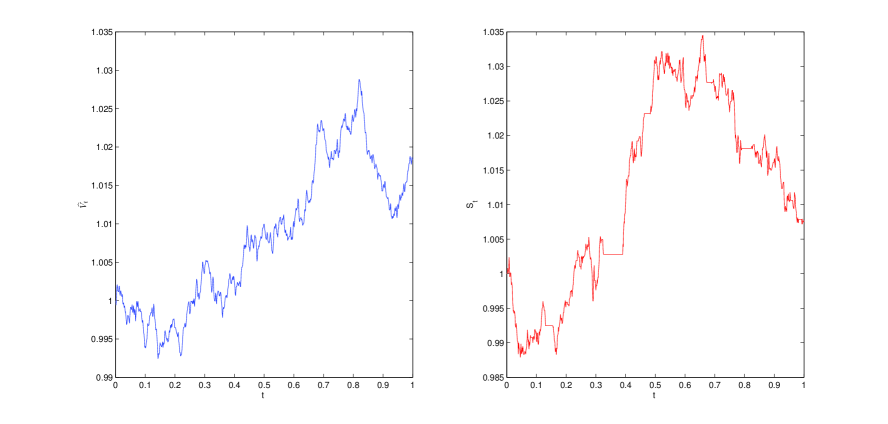
Fig. 2 shows typically the differences and relationships between the sample paths of the stock price in the F β B β M πΉ π΅ π FBM model and the subdiffusive F β B β M πΉ π΅ π FBM model.
Figure 1. Comparison of the sample paths of the stock price in the F β B β M πΉ π΅ π FBM model (left) and the subdiffusive F β B β M πΉ π΅ π FBM model (right) for r = 0.01 , Ξ± = 0.9 , H = 0.8 , Ο = 0.1 , S 0 = 1 formulae-sequence π 0.01 formulae-sequence πΌ 0.9 formulae-sequence π» 0.8 formulae-sequence π 0.1 subscript π 0 1 r=0.01,\alpha=0.9,H=0.8,\sigma=0.1,S_{0}=1 .
Here, assume that T Ξ± β ( t ) subscript π πΌ π‘ T_{\alpha}(t) is independent of B 1 H β ( Ο ) superscript subscript π΅ 1 π» π B_{1}^{H}(\tau) and B 2 H β ( Ο ) superscript subscript π΅ 2 π» π B_{2}^{H}(\tau) . Specially, when H = 1 2 π» 1 2 H=\frac{1}{2} , it is a subdiffusion process mentioned in Refs. [10 , 11 ] and when Ξ± β 1 β πΌ 1 \alpha\uparrow 1 , T Ξ± β ( t ) subscript π πΌ π‘ T_{\alpha}(t) reduces to physical time t π‘ t . In this study, we apply the subdiffusive mechanism of trapping events in order to describe financial data exhibiting periods of constant values.
This paper is organized as follows. In Section 2 , we derive the formula for the price of a riskless zero-coupon
bond paying $1 at maturity. In Section 3 , we obtain the corresponding B β S π΅ π BS equation by using delta hedging argument and discuss some special cases of this equation. In Section 4 , we present an
analytic pricing formula for the European call and put options. In Section 5 , we study some special properties of this pricing formula. Furthermore, we show how to use our model to price options by numerical simulations. The comparison of our model and traditional models is undertaken in
this section. Finally, Section 6 draws the concluding remarks.
2. Pricing formula for zero-coupon bond
The purpose of this section is to derive the pricing formula for zero-coupon bond P β ( r , t , T ) π π π‘ π P(r,t,T) . Here, P β ( r , T ; T ) = 1 π π π π 1 P(r,T;T)=1 , that is, the zero-coupon bond will pay
for 1 dollar at the expiry date T π T .
We assume that the short rate r β ( t ) π π‘ r(t) satisfy Equation (1.3 ), Ξ± β ( 1 2 , 1 ) πΌ 1 2 1 \alpha\in(\frac{1}{2},1) and 2 β Ξ± β Ξ± β H > 1 2 πΌ πΌ π» 1 2\alpha-\alpha H>1 , then by applying the Taylor series expansion to P β ( r , t , T ) π π π‘ π P(r,t,T) we obtain that
(2.1)
P β ( r + Ξ β r , t + Ξ β t ) π π Ξ π π‘ Ξ π‘ \displaystyle P(r+\Delta r,t+\Delta t)
= \displaystyle=
P β ( r , t , T ) + β P β r β Ξ β r + β P β t β Ξ β t π π π‘ π π π Ξ π π π‘ Ξ π‘ \displaystyle P(r,t,T)+\frac{\partial P}{\partial r}\Delta r+\frac{\partial P}{\partial t}\Delta t
+ 1 2 β 2 P β r 2 ( Ξ r ) 2 + + 1 2 β 2 P β r β β t Ξ r ( Ξ t ) + 1 2 β 2 P β t 2 ( Ξ t ) 2 + O ( Ξ t ) . \displaystyle+\frac{1}{2}\frac{\partial^{2}P}{\partial r^{2}}(\Delta r)^{2}++\frac{1}{2}\frac{\partial^{2}P}{\partial r\partial t}\Delta r(\Delta t)+\frac{1}{2}\frac{\partial^{2}P}{\partial t^{2}}(\Delta t)^{2}+O(\Delta t).
From, Equation (1.3 ) and [16 ] , we have
(2.2)
Ξ β r Ξ π \displaystyle\Delta r
= \displaystyle=
ΞΌ r β ( Ξ β T Ξ± β ( t ) ) + Ο r β B 1 H β ( T Ξ± β ( t ) ) subscript π π Ξ subscript π πΌ π‘ subscript π π superscript subscript π΅ 1 π» subscript π πΌ π‘ \displaystyle\mu_{r}(\Delta T_{\alpha}(t))+\sigma_{r}B_{1}^{H}(T_{\alpha}(t))
= \displaystyle=
ΞΌ r β ( t Ξ± β 1 Ξ β ( Ξ± ) ) 2 β H β ( Ξ β t ) 2 β H + Ο r β Ξ β B 1 H β ( T Ξ± β ( t ) ) + O β ( ( Ξ β t ) 2 β H ) . subscript π π superscript superscript π‘ πΌ 1 Ξ πΌ 2 π» superscript Ξ π‘ 2 π» subscript π π Ξ superscript subscript π΅ 1 π» subscript π πΌ π‘ π superscript Ξ π‘ 2 π» \displaystyle\mu_{r}\left(\frac{t^{\alpha-1}}{\Gamma(\alpha)}\right)^{2H}(\Delta t)^{2H}+\sigma_{r}\Delta B_{1}^{H}(T_{\alpha}(t))+O((\Delta t)^{2H}).
(2.3)
( Ξ β r ) 2 superscript Ξ π 2 \displaystyle(\Delta r)^{2}
= \displaystyle=
Ο r 2 β ( t Ξ± β 1 Ξ β ( Ξ± ) ) 2 β H β ( Ξ β t ) 2 β H + O β ( ( Ξ β t ) 2 β H ) . superscript subscript π π 2 superscript superscript π‘ πΌ 1 Ξ πΌ 2 π» superscript Ξ π‘ 2 π» π superscript Ξ π‘ 2 π» \displaystyle\sigma_{r}^{2}\left(\frac{t^{\alpha-1}}{\Gamma(\alpha)}\right)^{2H}(\Delta t)^{2H}+O((\Delta t)^{2H}).
(2.4)
Ξ β r β ( Ξ β t ) Ξ π Ξ π‘ \displaystyle\Delta r(\Delta t)
= \displaystyle=
O β ( ( Ξ β t ) 2 β H ) . π superscript Ξ π‘ 2 π» \displaystyle O((\Delta t)^{2H}).
Then from the Lemma 1 in [16 ] , we can get
(2.5)
d β P β ( r , t , T ) π π π π‘ π \displaystyle dP(r,t,T)
= \displaystyle=
[ ( t Ξ± β 1 Ξ β ( Ξ± ) ) 2 β H β ( ΞΌ r β β P β r + 1 2 β Ο r 2 β β 2 P β r 2 ) β 2 β H β t 2 β H β 1 + β P β t ] β d β t delimited-[] superscript superscript π‘ πΌ 1 Ξ πΌ 2 π» subscript π π π π 1 2 superscript subscript π π 2 superscript 2 π superscript π 2 2 π» superscript π‘ 2 π» 1 π π‘ π π‘ \displaystyle\left[\left(\frac{t^{\alpha-1}}{\Gamma(\alpha)}\right)^{2H}\left(\mu_{r}\frac{\partial P}{\partial r}+\frac{1}{2}\sigma_{r}^{2}\frac{\partial^{2}P}{\partial r^{2}}\right)2Ht^{2H-1}+\frac{\partial P}{\partial t}\right]dt
+ Ο r β β P β t β d β B 1 H β ( T Ξ± β ( t ) ) . subscript π π π π‘ π superscript subscript π΅ 1 π» subscript π πΌ π‘ \displaystyle+\sigma_{r}\frac{\partial P}{\partial t}dB_{1}^{H}(T_{\alpha}(t)).
Assuming
ΞΌ π \displaystyle\mu
= \displaystyle=
1 P β [ ( t Ξ± β 1 Ξ β ( Ξ± ) ) 2 β H β ( ΞΌ r β β P β r + 1 2 β Ο r 2 β β 2 P β r 2 ) β 2 β H β t 2 β H β 1 + β P β t ] , 1 π delimited-[] superscript superscript π‘ πΌ 1 Ξ πΌ 2 π» subscript π π π π 1 2 superscript subscript π π 2 superscript 2 π superscript π 2 2 π» superscript π‘ 2 π» 1 π π‘ \displaystyle\frac{1}{P}\left[\left(\frac{t^{\alpha-1}}{\Gamma(\alpha)}\right)^{2H}\left(\mu_{r}\frac{\partial P}{\partial r}+\frac{1}{2}\sigma_{r}^{2}\frac{\partial^{2}P}{\partial r^{2}}\right)2Ht^{2H-1}+\frac{\partial P}{\partial t}\right],
(2.6)
Ο π \displaystyle\sigma
= \displaystyle=
1 P β ( β P β r ) , 1 π π π \displaystyle\frac{1}{P}\left(\frac{\partial P}{\partial r}\right),
and letting the local expectations hypothesis holds for the term structure of interest rates
(i.e. ΞΌ = r π π \mu=r ), we obtain
β P β t + 2 β H β t 2 β H β 1 β ΞΌ r β ( t Ξ± β 1 Ξ β ( Ξ± ) ) 2 β H β β P β r π π‘ 2 π» superscript π‘ 2 π» 1 subscript π π superscript superscript π‘ πΌ 1 Ξ πΌ 2 π» π π \displaystyle\frac{\partial P}{\partial t}+2Ht^{2H-1}\mu_{r}\left(\frac{t^{\alpha-1}}{\Gamma(\alpha)}\right)^{2H}\frac{\partial P}{\partial r}
(2.7)
+ H β t 2 β H β 1 β Ο r 2 β ( t Ξ± β 1 Ξ β ( Ξ± ) ) 2 β H β β 2 P β r 2 β r β P = 0 . π» superscript π‘ 2 π» 1 superscript subscript π π 2 superscript superscript π‘ πΌ 1 Ξ πΌ 2 π» superscript 2 π superscript π 2 π π 0 \displaystyle+Ht^{2H-1}\sigma_{r}^{2}\left(\frac{t^{\alpha-1}}{\Gamma(\alpha)}\right)^{2H}\frac{\partial^{2}P}{\partial r^{2}}-rP=0.
Then, zero-coupon bond P β ( r , t , T ) π π π‘ π P(r,t,T) with boundary condition P β ( r , t , T ) = 1 π π π‘ π 1 P(r,t,T)=1 satisfy the following partial differential equation
β P β t + 2 β H β t 2 β H β 1 β ΞΌ r β ( t Ξ± β 1 Ξ β ( Ξ± ) ) 2 β H β β P β r π π‘ 2 π» superscript π‘ 2 π» 1 subscript π π superscript superscript π‘ πΌ 1 Ξ πΌ 2 π» π π \displaystyle\frac{\partial P}{\partial t}+2Ht^{2H-1}\mu_{r}\left(\frac{t^{\alpha-1}}{\Gamma(\alpha)}\right)^{2H}\frac{\partial P}{\partial r}
(2.8)
+ H β t 2 β H β 1 β Ο r 2 β ( t Ξ± β 1 Ξ β ( Ξ± ) ) 2 β H β β 2 P β r 2 β r β P = 0 . π» superscript π‘ 2 π» 1 superscript subscript π π 2 superscript superscript π‘ πΌ 1 Ξ πΌ 2 π» superscript 2 π superscript π 2 π π 0 \displaystyle+Ht^{2H-1}\sigma_{r}^{2}\left(\frac{t^{\alpha-1}}{\Gamma(\alpha)}\right)^{2H}\frac{\partial^{2}P}{\partial r^{2}}-rP=0.
To solve Equation (2.8 ) for P β ( r , t , T ) π π π‘ π P(r,t,T) , let Ο = T β t , P β ( r , t , T ) = exp β‘ { f 1 β ( Ο ) β r β f 2 β ( Ο ) } formulae-sequence π π π‘ π π π‘ π subscript π 1 π π subscript π 2 π \tau=T-t,P(r,t,T)=\exp\{f_{1}(\tau)-rf_{2}(\tau)\} , then we have
(2.9)
β P β t π π‘ \displaystyle\frac{\partial P}{\partial t}
= \displaystyle=
P β ( β β f 1 β ( Ο ) β t + r β β f 2 β ( Ο ) β t ) , π subscript π 1 π π‘ π subscript π 2 π π‘ \displaystyle P\left(-\frac{\partial f_{1}(\tau)}{\partial t}+r\frac{\partial f_{2}(\tau)}{\partial t}\right),
(2.10)
β P β r π π \displaystyle\frac{\partial P}{\partial r}
= \displaystyle=
β P β f 2 β ( Ο ) , π subscript π 2 π \displaystyle-Pf_{2}(\tau),
(2.11)
β 2 P β r 2 superscript 2 π superscript π 2 \displaystyle\frac{\partial^{2}P}{\partial r^{2}}
= \displaystyle=
P β f 2 β ( Ο ) 2 . π subscript π 2 superscript π 2 \displaystyle Pf_{2}(\tau)^{2}.
Substituting Equations (2.10 ) and (2.11 ) into Equation (2.9 ) and simplifying Equation (2.8 ) becomes
P [ H t 2 β H β 1 Ο r 2 f 2 ( Ο ) 2 ( t Ξ± β 1 Ξ β ( Ξ± ) ) 2 β H β 2 H t 2 β H β 1 ΞΌ r f 2 ( Ο ) ( t Ξ± β 1 Ξ β ( Ξ± ) ) 2 β H \displaystyle P\Bigg{[}Ht^{2H-1}\sigma_{r}^{2}f_{2}(\tau)^{2}\left(\frac{t^{\alpha-1}}{\Gamma(\alpha)}\right)^{2H}-2Ht^{2H-1}\mu_{r}f_{2}(\tau)\left(\frac{t^{\alpha-1}}{\Gamma(\alpha)}\right)^{2H}
(2.12)
β β f 1 β ( Ο ) β Ο + r ( β f 2 β ( Ο ) β t β 1 ) ] = 0 . \displaystyle-\frac{\partial f_{1}(\tau)}{\partial\tau}+r\left(\frac{\partial f_{2}(\tau)}{\partial t}-1\right)\Bigg{]}=0.
From Equation (2.12 ), we have
β f 1 β ( Ο ) β Ο subscript π 1 π π \displaystyle\frac{\partial f_{1}(\tau)}{\partial\tau}
= \displaystyle=
H β t 2 β H β 1 β ( t Ξ± β 1 Ξ β ( Ξ± ) ) 2 β H β ( Ο r 2 β f 2 β ( Ο ) 2 β 2 β ΞΌ r β f 2 β ( Ο ) ) , π» superscript π‘ 2 π» 1 superscript superscript π‘ πΌ 1 Ξ πΌ 2 π» superscript subscript π π 2 subscript π 2 superscript π 2 2 subscript π π subscript π 2 π \displaystyle Ht^{2H-1}\left(\frac{t^{\alpha-1}}{\Gamma(\alpha)}\right)^{2H}\left(\sigma_{r}^{2}f_{2}(\tau)^{2}-2\mu_{r}f_{2}(\tau)\right),
(2.13)
β f 2 β ( Ο ) β Ο subscript π 2 π π \displaystyle\frac{\partial f_{2}(\tau)}{\partial\tau}
= \displaystyle=
1 . 1 \displaystyle 1.
(2.14)
f 1 β ( Ο ) subscript π 1 π \displaystyle f_{1}(\tau)
= \displaystyle=
H β Ο r 2 ( Ξ β ( Ξ± ) ) 2 β H β β« 0 Ο ( T β s ) ( Ξ± β 1 ) β 2 β H + 2 β H β 1 β s 2 β π s π» superscript subscript π π 2 superscript Ξ πΌ 2 π» superscript subscript 0 π superscript π π πΌ 1 2 π» 2 π» 1 superscript π 2 differential-d π \displaystyle\frac{H\sigma_{r}^{2}}{(\Gamma(\alpha))^{2H}}\int_{0}^{\tau}(T-s)^{(\alpha-1)2H+2H-1}s^{2}ds
β 2 β H β ΞΌ r ( Ξ β ( Ξ± ) ) 2 β H β β« 0 Ο ( T β s ) ( Ξ± β 1 ) β 2 β H + 2 β H β 1 β s β π s , 2 π» subscript π π superscript Ξ πΌ 2 π» superscript subscript 0 π superscript π π πΌ 1 2 π» 2 π» 1 π differential-d π \displaystyle-\frac{2H\mu_{r}}{(\Gamma(\alpha))^{2H}}\int_{0}^{\tau}(T-s)^{(\alpha-1)2H+2H-1}sds,
(2.15)
f 2 β ( Ο ) subscript π 2 π \displaystyle f_{2}(\tau)
= \displaystyle=
Ο . π \displaystyle\tau.
Hence, we obtain a formula for the price at time t π‘ t of a riskless zero-coupon bond which
pay $1 at maturity T π T is given by
(2.16)
P β ( r , t , T ) = e β r β Ο + f 1 β ( Ο ) . π π π‘ π superscript π π π subscript π 1 π \displaystyle P(r,t,T)=e^{-r\tau+f_{1}(\tau)}.
Corollary 2.1 .
When Ξ± β 1 β πΌ 1 \alpha\uparrow 1 , Equations (1.3 ) and (1.4 ) reduce to the F β B β M πΉ π΅ π FBM , we obtain
(2.17)
f 1 β ( Ο ) subscript π 1 π \displaystyle f_{1}(\tau)
= \displaystyle=
H β Ο r 2 β β« 0 Ο ( T β s ) 2 β H β 1 β s 2 β π s β 2 β H β ΞΌ r β β« 0 Ο ( T β s ) 2 β H β 1 β s β π s , π» superscript subscript π π 2 superscript subscript 0 π superscript π π 2 π» 1 superscript π 2 differential-d π 2 π» subscript π π superscript subscript 0 π superscript π π 2 π» 1 π differential-d π \displaystyle H\sigma_{r}^{2}\int_{0}^{\tau}(T-s)^{2H-1}s^{2}ds-2H\mu_{r}\int_{0}^{\tau}(T-s)^{2H-1}sds,
specially, if t = 0 π‘ 0 t=0
(2.18)
f 1 β ( Ο ) subscript π 1 π \displaystyle f_{1}(\tau)
= \displaystyle=
Ο r 2 β T 2 β H + 2 ( 2 β H + 1 ) β ( 2 β H + 2 ) β ΞΌ r β T 2 β H + 1 2 β H + 1 , superscript subscript π π 2 superscript π 2 π» 2 2 π» 1 2 π» 2 subscript π π superscript π 2 π» 1 2 π» 1 \displaystyle\sigma_{r}^{2}\frac{T^{2H+2}}{(2H+1)(2H+2)}-\mu_{r}\frac{T^{2H+1}}{2H+1},
then
(2.19)
P β ( r , t , T ) = exp β‘ { β r β T + Ο r 2 β T 2 β H + 2 ( 2 β H + 1 ) β ( 2 β H + 2 ) β ΞΌ r β T 2 β H + 1 2 β H + 1 } . π π π‘ π π π superscript subscript π π 2 superscript π 2 π» 2 2 π» 1 2 π» 2 subscript π π superscript π 2 π» 1 2 π» 1 \displaystyle P(r,t,T)=\exp\left\{-rT+\sigma_{r}^{2}\frac{T^{2H+2}}{(2H+1)(2H+2)}-\mu_{r}\frac{T^{2H+1}}{2H+1}\right\}.
Corollary 2.2 .
If H = 1 2 π» 1 2 H=\frac{1}{2} , from Equation (2.14 ), we obtain
(2.20)
f 1 β ( Ο ) subscript π 1 π \displaystyle f_{1}(\tau)
= \displaystyle=
1 2 β Ο r 2 Ξ β ( Ξ± ) β β« 0 Ο ( T β s ) Ξ± β 1 β s 2 β π s 1 2 superscript subscript π π 2 Ξ πΌ superscript subscript 0 π superscript π π πΌ 1 superscript π 2 differential-d π \displaystyle\frac{1}{2}\frac{\sigma_{r}^{2}}{\Gamma(\alpha)}\int_{0}^{\tau}(T-s)^{\alpha-1}s^{2}ds
β ΞΌ r Ξ β ( Ξ± ) β β« 0 Ο ( T β s ) Ξ± β 1 β s β π s , subscript π π Ξ πΌ superscript subscript 0 π superscript π π πΌ 1 π differential-d π \displaystyle-\frac{\mu_{r}}{\Gamma(\alpha)}\int_{0}^{\tau}(T-s)^{\alpha-1}sds,
then the result is consistent with the result in [5 ] .
Further, if Ξ± β 1 β πΌ 1 \alpha\uparrow 1 and H = 1 2 π» 1 2 H=\frac{1}{2} , Equations (1.3 ) and (1.4 ) reduce to the geometric Brownian motion, then we have
(2.21)
f 1 β ( Ο ) = 1 6 β Ο r 2 β Ο 3 β 1 2 β ΞΌ r β Ο 2 , subscript π 1 π 1 6 superscript subscript π π 2 superscript π 3 1 2 subscript π π superscript π 2 \displaystyle f_{1}(\tau)=\frac{1}{6}\sigma_{r}^{2}\tau^{3}-\frac{1}{2}\mu_{r}\tau^{2},
then
(2.22)
P β ( r , t , T ) = e β r β Ο + 1 6 β Ο r 2 β Ο 3 β 1 2 β ΞΌ r β Ο 2 . π π π‘ π superscript π π π 1 6 superscript subscript π π 2 superscript π 3 1 2 subscript π π superscript π 2 \displaystyle P(r,t,T)=e^{-r\tau+\frac{1}{6}\sigma_{r}^{2}\tau^{3}-\frac{1}{2}\mu_{r}\tau^{2}}.
which is consistent with the result in [7 , 3 ] .
3. Fractional B β S π΅ π BS equation
The purpose of this section is to derive the fractional B β S π΅ π BS equation for European options when the short rate r β ( t ) π π‘ r(t) and stock price S ( T ) = S ( T Ξ± ( t ) S(T)=S(T_{\alpha}(t) satisfy Equations (1.3 ) and (1.4 ), respectively. We assume that B 1 H β ( T Ξ± β ( t ) ) superscript subscript π΅ 1 π» subscript π πΌ π‘ B_{1}^{H}(T_{\alpha}(t)) and B 2 H β ( T Ξ± β ( t ) ) superscript subscript π΅ 2 π» subscript π πΌ π‘ B_{2}^{H}(T_{\alpha}(t)) are two F β B β M πΉ π΅ π FBM with Hurst parameter H β [ 1 2 , 1 ) π» 1 2 1 H\in[\frac{1}{2},1) and correlation coefficient Ο π \rho .
Let C = C β ( S , r , t ) πΆ πΆ π π π‘ C=C(S,r,t) be the price of a European call option at time t with a strike price K πΎ K that matures at time T π T . Then we
have.
Theorem 3.1 .
Assume that the stock price short rate r β ( t ) π π‘ r(t) and S β ( t ) π π‘ S(t) satisfy Equations (1.3 ) and (1.4 ), respectively. Then, C β ( S , r , t ) πΆ π π π‘ C(S,r,t) satisfies the following fractional B β S π΅ π BS equation
β C β t + Ο ~ s 2 β ( t ) β S 2 β β 2 C β S 2 + Ο ~ r 2 β ( t ) β β 2 C β r 2 + 2 β Ο β Ο ~ r β ( t ) β Ο ~ s β ( t ) β β 2 C β S β β r πΆ π‘ superscript subscript ~ π π 2 π‘ superscript π 2 superscript 2 πΆ superscript π 2 superscript subscript ~ π π 2 π‘ superscript 2 πΆ superscript π 2 2 π subscript ~ π π π‘ subscript ~ π π π‘ superscript 2 πΆ π π \displaystyle\frac{\partial C}{\partial t}+\widetilde{\sigma}_{s}^{2}(t)S^{2}\frac{\partial^{2}C}{\partial S^{2}}+\widetilde{\sigma}_{r}^{2}(t)\frac{\partial^{2}C}{\partial r^{2}}+2\rho\widetilde{\sigma}_{r}(t)\widetilde{\sigma}_{s}(t)\frac{\partial^{2}C}{\partial S\partial r}
(3.1)
+ 2 β H β t 2 β H β 1 β ΞΌ r β ( t Ξ± β 1 Ξ β ( Ξ± ) ) 2 β H β β C β r + r β S β β C β S β r β C = 0 , 2 π» superscript π‘ 2 π» 1 subscript π π superscript superscript π‘ πΌ 1 Ξ πΌ 2 π» πΆ π π π πΆ π π πΆ 0 \displaystyle+2Ht^{2H-1}\mu_{r}\left(\frac{t^{\alpha-1}}{\Gamma(\alpha)}\right)^{2H}\frac{\partial C}{\partial r}+rS\frac{\partial C}{\partial S}-rC=0,
where
(3.2)
Ο ~ s 2 β ( t ) = H β t 2 β H β 1 β Ο s 2 β ( t Ξ± β 1 Ξ β ( Ξ± ) ) 2 β H , superscript subscript ~ π π 2 π‘ π» superscript π‘ 2 π» 1 superscript subscript π π 2 superscript superscript π‘ πΌ 1 Ξ πΌ 2 π» \displaystyle\widetilde{\sigma}_{s}^{2}(t)=Ht^{2H-1}\sigma_{s}^{2}\left(\frac{t^{\alpha-1}}{\Gamma(\alpha)}\right)^{2H},
(3.3)
Ο ~ r 2 β ( t ) = H β t 2 β H β 1 β Ο r 2 β ( t Ξ± β 1 Ξ β ( Ξ± ) ) 2 β H . superscript subscript ~ π π 2 π‘ π» superscript π‘ 2 π» 1 superscript subscript π π 2 superscript superscript π‘ πΌ 1 Ξ πΌ 2 π» \displaystyle\widetilde{\sigma}_{r}^{2}(t)=Ht^{2H-1}\sigma_{r}^{2}\left(\frac{t^{\alpha-1}}{\Gamma(\alpha)}\right)^{2H}.
Ο s , Ο r , ΞΌ s , ΞΌ s , subscript π π subscript π π subscript π π subscript π π
\sigma_{s},\sigma_{r},\mu_{s},\mu_{s}, are constant, H β [ 1 2 , 1 ) π» 1 2 1 H\in[\frac{1}{2},1) and Ξ± β ( 1 2 , 1 ) πΌ 1 2 1 \alpha\in(\frac{1}{2},1) and 2 β Ξ± β Ξ± β H > 1 2 πΌ πΌ π» 1 2\alpha-\alpha H>1 .
Proof:
We consider a portfolio with D 1 β t subscript π· 1 π‘ D_{1t} units of stock and D 2 β t subscript π· 2 π‘ D_{2t} units of zero-coupon bond P β ( r , t , T ) π π π‘ π P(r,t,T) and one unit of C = C β ( r , t , T ) πΆ πΆ π π‘ π C=C(r,t,T) . Then,
the value of the portfolio at current time t π‘ t is
(3.4)
Ξ t = C β D 1 β t β S t β D 2 β t β P t . subscript Ξ π‘ πΆ subscript π· 1 π‘ subscript π π‘ subscript π· 2 π‘ subscript π π‘ \displaystyle\Pi_{t}=C-D_{1t}S_{t}-D_{2t}P_{t}.
Then, from [5 ] we have
(3.5)
d β Ξ t π subscript Ξ π‘ \displaystyle d\Pi_{t}
= \displaystyle=
C t β D 1 β t β d β S t β D 2 β t β d β P t subscript πΆ π‘ subscript π· 1 π‘ π subscript π π‘ subscript π· 2 π‘ π subscript π π‘ \displaystyle C_{t}-D_{1t}dS_{t}-D_{2t}dP_{t}
= \displaystyle=
[ β C β t d t + H t 2 β H β 1 Ο s 2 S t 2 ( t Ξ± β 1 Ξ β ( Ξ± ) ) 2 β H β 2 C β S 2 + H t 2 β H β 1 Ο r 2 ( t Ξ± β 1 Ξ β ( Ξ± ) ) 2 β H β 2 C β r 2 \displaystyle\Bigg{[}\frac{\partial C}{\partial t}dt+Ht^{2H-1}\sigma_{s}^{2}S_{t}^{2}\left(\frac{t^{\alpha-1}}{\Gamma(\alpha)}\right)^{2H}\frac{\partial^{2}C}{\partial S^{2}}+Ht^{2H-1}\sigma_{r}^{2}\left(\frac{t^{\alpha-1}}{\Gamma(\alpha)}\right)^{2H}\frac{\partial^{2}C}{\partial r^{2}}
+ \displaystyle+
2 H t 2 β H β 1 Ο Ο r Ο s S ( t Ξ± β 1 Ξ β ( Ξ± ) ) 2 β H β 2 C β S β β r ] d t + [ β C β t β D 1 β t ] d S t \displaystyle 2Ht^{2H-1}\rho\sigma_{r}\sigma_{s}S\left(\frac{t^{\alpha-1}}{\Gamma(\alpha)}\right)^{2H}\frac{\partial^{2}C}{\partial S\partial r}\Bigg{]}dt+\Bigg{[}\frac{\partial C}{\partial t}-D_{1t}\Bigg{]}dS_{t}
+ \displaystyle+
[ β C β r β D 2 β t β β P β r ] β d β r + D 2 β t β [ β P β t + H β t 2 β H β 1 β Ο r 2 β ( t Ξ± β 1 Ξ β ( Ξ± ) ) 2 β H β β 2 P β r 2 ] β d β t . delimited-[] πΆ π subscript π· 2 π‘ π π π π subscript π· 2 π‘ delimited-[] π π‘ π» superscript π‘ 2 π» 1 superscript subscript π π 2 superscript superscript π‘ πΌ 1 Ξ πΌ 2 π» superscript 2 π superscript π 2 π π‘ \displaystyle\Bigg{[}\frac{\partial C}{\partial r}-D_{2t}\frac{\partial P}{\partial r}\Bigg{]}dr+D_{2t}\Bigg{[}\frac{\partial P}{\partial t}+Ht^{2H-1}\sigma_{r}^{2}\left(\frac{t^{\alpha-1}}{\Gamma(\alpha)}\right)^{2H}\frac{\partial^{2}P}{\partial r^{2}}\Bigg{]}dt.
By setting D 1 β t = β C β S , D 2 β t = β C β r β P β r , formulae-sequence subscript π· 1 π‘ πΆ π subscript π· 2 π‘ πΆ π π π D_{1t}=\frac{\partial C}{\partial S},\,D_{2t}=\frac{\frac{\partial C}{\partial r}}{\frac{\partial P}{\partial r}}, to eliminate the stochastic noise, then
(3.6)
d β Ξ t π subscript Ξ π‘ \displaystyle d\Pi_{t}
= \displaystyle=
= \displaystyle=
[ β C β t + H β t 2 β H β 1 β ( t Ξ± β 1 Ξ β ( Ξ± ) ) 2 β H β ( Ο s 2 β S 2 β β 2 C β S 2 + Ο r 2 β β 2 C β r 2 + 2 β Ο β Ο r β Ο s β S β β 2 C β S β β r ) ] β d β t delimited-[] πΆ π‘ π» superscript π‘ 2 π» 1 superscript superscript π‘ πΌ 1 Ξ πΌ 2 π» superscript subscript π π 2 superscript π 2 superscript 2 πΆ superscript π 2 superscript subscript π π 2 superscript 2 πΆ superscript π 2 2 π subscript π π subscript π π π superscript 2 πΆ π π π π‘ \displaystyle\Bigg{[}\frac{\partial C}{\partial t}+Ht^{2H-1}\left(\frac{t^{\alpha-1}}{\Gamma(\alpha)}\right)^{2H}\left(\sigma_{s}^{2}S^{2}\frac{\partial^{2}C}{\partial S^{2}}+\sigma_{r}^{2}\frac{\partial^{2}C}{\partial r^{2}}+2\rho\sigma_{r}\sigma_{s}S\frac{\partial^{2}C}{\partial S\partial r}\right)\Bigg{]}dt
β \displaystyle-
β C β r β P β r β [ r β P β 2 β H β t 2 β H β 1 β ΞΌ r β ( t Ξ± β 1 Ξ β ( Ξ± ) ) 2 β H β β P β r ] β d β t . πΆ π π π delimited-[] π π 2 π» superscript π‘ 2 π» 1 subscript π π superscript superscript π‘ πΌ 1 Ξ πΌ 2 π» π π π π‘ \displaystyle\frac{\frac{\partial C}{\partial r}}{\frac{\partial P}{\partial r}}\Bigg{[}rP-2Ht^{2H-1}\mu_{r}\left(\frac{t^{\alpha-1}}{\Gamma(\alpha)}\right)^{2H}\frac{\partial P}{\partial r}\Bigg{]}dt.
The return of an amount Ξ t subscript Ξ π‘ \Pi_{t} invested in bank account
is equal to r β ( t ) β Ξ t β d β t π π‘ subscript Ξ π‘ π π‘ r(t)\Pi_{t}dt at time d β t π π‘ dt , πΌ β ( d β Ξ t ) = r β ( t ) β Ξ t β d β t = r β ( t ) β ( C β D 1 β t β S t β D 2 β t β P t ) πΌ π subscript Ξ π‘ π π‘ subscript Ξ π‘ π π‘ π π‘ πΆ subscript π· 1 π‘ subscript π π‘ subscript π· 2 π‘ subscript π π‘ \mathbb{E}(d\Pi_{t})=r(t)\Pi_{t}dt=r(t)\left(C-D_{1t}S_{t}-D_{2t}P_{t}\right) , hence from Equation (3.6 ) we have
β C β t + H β t 2 β H β 1 β ( t Ξ± β 1 Ξ β ( Ξ± ) ) 2 β H β ( Ο s 2 β S 2 β β 2 C β S 2 + Ο r 2 β β 2 C β r 2 + 2 β Ο β Ο r β Ο s β S β β 2 C β S β β r ) πΆ π‘ π» superscript π‘ 2 π» 1 superscript superscript π‘ πΌ 1 Ξ πΌ 2 π» superscript subscript π π 2 superscript π 2 superscript 2 πΆ superscript π 2 superscript subscript π π 2 superscript 2 πΆ superscript π 2 2 π subscript π π subscript π π π superscript 2 πΆ π π \displaystyle\frac{\partial C}{\partial t}+Ht^{2H-1}\left(\frac{t^{\alpha-1}}{\Gamma(\alpha)}\right)^{2H}\left(\sigma_{s}^{2}S^{2}\frac{\partial^{2}C}{\partial S^{2}}+\sigma_{r}^{2}\frac{\partial^{2}C}{\partial r^{2}}+2\rho\sigma_{r}\sigma_{s}S\frac{\partial^{2}C}{\partial S\partial r}\right)
(3.7)
+ 2 β H β t 2 β H β 1 β ΞΌ r β ( t Ξ± β 1 Ξ β ( Ξ± ) ) 2 β H β β C β r + r β S β β C β S β r β C = 0 . 2 π» superscript π‘ 2 π» 1 subscript π π superscript superscript π‘ πΌ 1 Ξ πΌ 2 π» πΆ π π π πΆ π π πΆ 0 \displaystyle+2Ht^{2H-1}\mu_{r}\left(\frac{t^{\alpha-1}}{\Gamma(\alpha)}\right)^{2H}\frac{\partial C}{\partial r}+rS\frac{\partial C}{\partial S}-rC=0.
Let
(3.8)
Ο ~ s 2 β ( t ) = H β t 2 β H β 1 β Ο s 2 β ( t Ξ± β 1 Ξ β ( Ξ± ) ) 2 β H , superscript subscript ~ π π 2 π‘ π» superscript π‘ 2 π» 1 superscript subscript π π 2 superscript superscript π‘ πΌ 1 Ξ πΌ 2 π» \displaystyle\widetilde{\sigma}_{s}^{2}(t)=Ht^{2H-1}\sigma_{s}^{2}\left(\frac{t^{\alpha-1}}{\Gamma(\alpha)}\right)^{2H},
(3.9)
Ο ~ r 2 β ( t ) = H β t 2 β H β 1 β Ο r 2 β ( t Ξ± β 1 Ξ β ( Ξ± ) ) 2 β H . superscript subscript ~ π π 2 π‘ π» superscript π‘ 2 π» 1 superscript subscript π π 2 superscript superscript π‘ πΌ 1 Ξ πΌ 2 π» \displaystyle\widetilde{\sigma}_{r}^{2}(t)=Ht^{2H-1}\sigma_{r}^{2}\left(\frac{t^{\alpha-1}}{\Gamma(\alpha)}\right)^{2H}.
Then
β C β t + Ο ~ s 2 β ( t ) β S t 2 β β 2 C β S t 2 + Ο ~ r 2 β ( t ) β β 2 C β r 2 + 2 β Ο β Ο ~ r β ( t ) β Ο ~ s β ( t ) β β 2 C β S β β r πΆ π‘ superscript subscript ~ π π 2 π‘ superscript subscript π π‘ 2 superscript 2 πΆ superscript subscript π π‘ 2 superscript subscript ~ π π 2 π‘ superscript 2 πΆ superscript π 2 2 π subscript ~ π π π‘ subscript ~ π π π‘ superscript 2 πΆ π π \displaystyle\frac{\partial C}{\partial t}+\widetilde{\sigma}_{s}^{2}(t)S_{t}^{2}\frac{\partial^{2}C}{\partial S_{t}^{2}}+\widetilde{\sigma}_{r}^{2}(t)\frac{\partial^{2}C}{\partial r^{2}}+2\rho\widetilde{\sigma}_{r}(t)\widetilde{\sigma}_{s}(t)\frac{\partial^{2}C}{\partial S\partial r}
(3.10)
+ 2 β H β t 2 β H β 1 β ΞΌ r β ( t Ξ± β 1 Ξ β ( Ξ± ) ) 2 β H β β C β r + r β S β β C β S β r β C = 0 , 2 π» superscript π‘ 2 π» 1 subscript π π superscript superscript π‘ πΌ 1 Ξ πΌ 2 π» πΆ π π π πΆ π π πΆ 0 \displaystyle+2Ht^{2H-1}\mu_{r}\left(\frac{t^{\alpha-1}}{\Gamma(\alpha)}\right)^{2H}\frac{\partial C}{\partial r}+rS\frac{\partial C}{\partial S}-rC=0,
From Theorem (3.1 ), we can get the following corollaries
Corollary 3.1 .
If Ο = 0 π 0 \rho=0 and r β ( t ) π π‘ r(t) be a constant, then the European call option C = C β ( S , r , T ) πΆ πΆ π π π C=C(S,r,T) satisfies
(3.11)
β C β t + H β t 2 β H β 1 β Ο s 2 β S t 2 β ( t Ξ± β 1 Ξ β ( Ξ± ) ) 2 β H β β 2 C β S t 2 + r β S β β C β S β r β C = 0 , πΆ π‘ π» superscript π‘ 2 π» 1 superscript subscript π π 2 superscript subscript π π‘ 2 superscript superscript π‘ πΌ 1 Ξ πΌ 2 π» superscript 2 πΆ superscript subscript π π‘ 2 π π πΆ π π πΆ 0 \displaystyle\frac{\partial C}{\partial t}+Ht^{2H-1}\sigma_{s}^{2}S_{t}^{2}\left(\frac{t^{\alpha-1}}{\Gamma(\alpha)}\right)^{2H}\frac{\partial^{2}C}{\partial S_{t}^{2}}+rS\frac{\partial C}{\partial S}-rC=0,
which is a fractional B β S π΅ π BS equation considered in [8 ] .
Corollary 3.2 .
When Ξ± β 1 β πΌ 1 \alpha\uparrow 1 , we obtain
β C β t + H β t 2 β H β 1 β Ο s 2 β S t 2 β β 2 C β S t 2 + H β t 2 β H β 1 β Ο r 2 β β 2 C β r 2 + 2 β H β t 2 β H β 1 β Ο β Ο r β Ο s β β 2 C β S β β r πΆ π‘ π» superscript π‘ 2 π» 1 superscript subscript π π 2 superscript subscript π π‘ 2 superscript 2 πΆ superscript subscript π π‘ 2 π» superscript π‘ 2 π» 1 superscript subscript π π 2 superscript 2 πΆ superscript π 2 2 π» superscript π‘ 2 π» 1 π subscript π π subscript π π superscript 2 πΆ π π \displaystyle\frac{\partial C}{\partial t}+Ht^{2H-1}\sigma_{s}^{2}S_{t}^{2}\frac{\partial^{2}C}{\partial S_{t}^{2}}+Ht^{2H-1}\sigma_{r}^{2}\frac{\partial^{2}C}{\partial r^{2}}+2Ht^{2H-1}\rho\sigma_{r}\sigma_{s}\frac{\partial^{2}C}{\partial S\partial r}
(3.12)
+ 2 β H β t 2 β H β 1 β ΞΌ r β β C β r + r β S β β C β S β r β C = 0 , 2 π» superscript π‘ 2 π» 1 subscript π π πΆ π π π πΆ π π πΆ 0 \displaystyle+2Ht^{2H-1}\mu_{r}\frac{\partial C}{\partial r}+rS\frac{\partial C}{\partial S}-rC=0,
Further, if Ο = 0 π 0 \rho=0 , H = 1 2 π» 1 2 H=\frac{1}{2} , and r β ( t ) π π‘ r(t) be a constant, from Equation (3.12 ) we have the celebrated B β S π΅ π BS equation
(3.13)
β C β t + 1 2 β Ο s 2 β S t 2 β β 2 C β S t 2 + r β S β β C β S β r β C = 0 , πΆ π‘ 1 2 superscript subscript π π 2 superscript subscript π π‘ 2 superscript 2 πΆ superscript subscript π π‘ 2 π π πΆ π π πΆ 0 \displaystyle\frac{\partial C}{\partial t}+\frac{1}{2}\sigma_{s}^{2}S_{t}^{2}\frac{\partial^{2}C}{\partial S_{t}^{2}}+rS\frac{\partial C}{\partial S}-rC=0,
4. Pricing formula under subdiffusive fractional Merton short rate model
In this section, we propose an explicit formula for European call option when its value satisfy the partial differential equation (3.1 ) with boundary condition C β ( S , r , T ) = ( S T β K ) + πΆ π π π superscript subscript π π πΎ C(S,r,T)=(S_{T}-K)^{+} . Then, we can get
Theorem 4.1 .
Let r β ( t ) π π‘ r(t) satisfies Equation (1.3 ) and S β ( t ) π π‘ S(t) satisfies Equation (1.4 ), then the price of European call and put options with strike price K πΎ K and maturity T π T are given by
(4.1)
C β ( S , r , t ) πΆ π π π‘ \displaystyle C(S,r,t)
= \displaystyle=
S β Ο β ( d 1 ) β K β P β ( r , t , T ) β Ο β ( d 2 ) , π italic-Ο subscript π 1 πΎ π π π‘ π italic-Ο subscript π 2 \displaystyle S\phi(d_{1})-KP(r,t,T)\phi(d_{2}),
(4.2)
P β ( S , r , t ) π π π π‘ \displaystyle P(S,r,t)
= \displaystyle=
K β P β ( r , t , T ) β Ο β ( β d 2 ) β Ο β ( β d 1 ) . πΎ π π π‘ π italic-Ο subscript π 2 italic-Ο subscript π 1 \displaystyle KP(r,t,T)\phi(-d_{2})-\phi(-d_{1}).
where
(4.3)
d 1 subscript π 1 \displaystyle d_{1}
= \displaystyle=
ln β‘ S K β ln β‘ P β ( r , t , T ) + H ( Ξ β ( Ξ± ) ) 2 β H β β« t T Ο ^ 2 β ( s ) β s ( Ξ± β 1 ) β 2 β H + 2 β H β 1 β π s 2 β H ( Ξ β ( Ξ± ) ) 2 β H β β« t T Ο ^ 2 β ( s ) β s ( Ξ± β 1 ) β 2 β H + 2 β H β 1 β π s , π πΎ π π π‘ π π» superscript Ξ πΌ 2 π» superscript subscript π‘ π superscript ^ π 2 π superscript π πΌ 1 2 π» 2 π» 1 differential-d π 2 π» superscript Ξ πΌ 2 π» superscript subscript π‘ π superscript ^ π 2 π superscript π πΌ 1 2 π» 2 π» 1 differential-d π \displaystyle\frac{\ln\frac{S}{K}-\ln P(r,t,T)+\frac{H}{(\Gamma(\alpha))^{2H}}\int_{t}^{T}\widehat{\sigma}^{2}(s)s^{(\alpha-1)2H+2H-1}ds}{\sqrt{\frac{2H}{(\Gamma(\alpha))^{2H}}\int_{t}^{T}\widehat{\sigma}^{2}(s)s^{(\alpha-1)2H+2H-1}ds}},
(4.4)
d 2 subscript π 2 \displaystyle d_{2}
= \displaystyle=
d 1 β 2 β H ( Ξ β ( Ξ± ) ) 2 β H β β« t T Ο ^ 2 β ( s ) β s ( Ξ± β 1 ) β 2 β H + 2 β H β 1 β π s , subscript π 1 2 π» superscript Ξ πΌ 2 π» superscript subscript π‘ π superscript ^ π 2 π superscript π πΌ 1 2 π» 2 π» 1 differential-d π \displaystyle d_{1}-\sqrt{\frac{2H}{(\Gamma(\alpha))^{2H}}\int_{t}^{T}\widehat{\sigma}^{2}(s)s^{(\alpha-1)2H+2H-1}ds},
(4.5)
Ο ^ 2 β ( t ) superscript ^ π 2 π‘ \displaystyle\widehat{\sigma}^{2}(t)
= \displaystyle=
Ο s 2 + 2 β Ο β Ο r β Ο s β ( T β t ) + Ο r 2 β ( T β t ) 2 . superscript subscript π π 2 2 π subscript π π subscript π π π π‘ superscript subscript π π 2 superscript π π‘ 2 \displaystyle\sigma_{s}^{2}+2\rho\sigma_{r}\sigma_{s}(T-t)+\sigma_{r}^{2}(T-t)^{2}.
P β ( r , t , T ) π π π‘ π P(r,t,T) is given by Equation (2.16 ) and Ο ( . ) \phi(.) is the cumulative normal distribution function.
Consider the partial differential equation (3.1 ) of the European call option with boundary condition C β ( S , r , T ) = ( S T β K ) + πΆ π π π superscript subscript π π πΎ C(S,r,T)=(S_{T}-K)^{+}
β C β t + Ο ~ s 2 β ( t ) β S t 2 β β 2 C β S t 2 + Ο ~ r 2 β ( t ) β β 2 C β r 2 + 2 β Ο β Ο ~ r β ( t ) β Ο ~ s β ( t ) β β 2 C β S β β r πΆ π‘ superscript subscript ~ π π 2 π‘ superscript subscript π π‘ 2 superscript 2 πΆ superscript subscript π π‘ 2 superscript subscript ~ π π 2 π‘ superscript 2 πΆ superscript π 2 2 π subscript ~ π π π‘ subscript ~ π π π‘ superscript 2 πΆ π π \displaystyle\frac{\partial C}{\partial t}+\widetilde{\sigma}_{s}^{2}(t)S_{t}^{2}\frac{\partial^{2}C}{\partial S_{t}^{2}}+\widetilde{\sigma}_{r}^{2}(t)\frac{\partial^{2}C}{\partial r^{2}}+2\rho\widetilde{\sigma}_{r}(t)\widetilde{\sigma}_{s}(t)\frac{\partial^{2}C}{\partial S\partial r}
(4.6)
+ 2 β H β t 2 β H β 1 β ΞΌ r β ( t Ξ± β 1 Ξ β ( Ξ± ) ) 2 β H β β C β r + r β S β β C β S β r β C = 0 . 2 π» superscript π‘ 2 π» 1 subscript π π superscript superscript π‘ πΌ 1 Ξ πΌ 2 π» πΆ π π π πΆ π π πΆ 0 \displaystyle+2Ht^{2H-1}\mu_{r}\left(\frac{t^{\alpha-1}}{\Gamma(\alpha)}\right)^{2H}\frac{\partial C}{\partial r}+rS\frac{\partial C}{\partial S}-rC=0.
Denote
(4.7)
z = S P β ( r , t , T ) , Ξ β ( z , t ) = C β ( S , r , t ) P β ( r , t , T ) , formulae-sequence π§ π π π π‘ π Ξ π§ π‘ πΆ π π π‘ π π π‘ π \displaystyle z=\frac{S}{P(r,t,T)},\quad\Theta(z,t)=\frac{C(S,r,t)}{P(r,t,T)},
therefore by computing, we get
β C β t πΆ π‘ \displaystyle\frac{\partial C}{\partial t}
= \displaystyle=
Ξ β β P β t + P β β Ξ β t β z β β Ξ β z β β P β t , Ξ π π‘ π Ξ π‘ π§ Ξ π§ π π‘ \displaystyle\Theta\frac{\partial P}{\partial t}+P\frac{\partial\Theta}{\partial t}-z\frac{\partial\Theta}{\partial z}\frac{\partial P}{\partial t},
β C β r πΆ π \displaystyle\frac{\partial C}{\partial r}
= \displaystyle=
Ξ β β P β r β z β β Ξ β z β β P β r , Ξ π π π§ Ξ π§ π π \displaystyle\Theta\frac{\partial P}{\partial r}-z\frac{\partial\Theta}{\partial z}\frac{\partial P}{\partial r},
(4.8)
β C β S πΆ π \displaystyle\frac{\partial C}{\partial S}
= \displaystyle=
β Ξ β z , Ξ π§ \displaystyle\frac{\partial\Theta}{\partial z},
β 2 C β r 2 superscript 2 πΆ superscript π 2 \displaystyle\frac{\partial^{2}C}{\partial r^{2}}
= \displaystyle=
Ξ β β 2 P β r 2 β z β β Ξ β z β β 2 P β r 2 + z 2 P β β 2 Ξ β z 2 β ( β P β r ) 2 , Ξ superscript 2 π superscript π 2 π§ Ξ π§ superscript 2 π superscript π 2 superscript π§ 2 π superscript 2 Ξ superscript π§ 2 superscript π π 2 \displaystyle\Theta\frac{\partial^{2}P}{\partial r^{2}}-z\frac{\partial\Theta}{\partial z}\frac{\partial^{2}P}{\partial r^{2}}+\frac{z^{2}}{P}\frac{\partial^{2}\Theta}{\partial z^{2}}\left(\frac{\partial P}{\partial r}\right)^{2},
β 2 C β r β β S superscript 2 πΆ π π \displaystyle\frac{\partial^{2}C}{\partial r\partial S}
= \displaystyle=
β z P β β 2 Ξ β z 2 β β P β r , π§ π superscript 2 Ξ superscript π§ 2 π π \displaystyle-\frac{z}{P}\frac{\partial^{2}\Theta}{\partial z^{2}}\frac{\partial P}{\partial r},
β 2 C β S 2 superscript 2 πΆ superscript π 2 \displaystyle\frac{\partial^{2}C}{\partial S^{2}}
= \displaystyle=
1 P β β 2 Ξ β z 2 . 1 π superscript 2 Ξ superscript π§ 2 \displaystyle\frac{1}{P}\frac{\partial^{2}\Theta}{\partial z^{2}}.
Inserting Equation (4.8 ) into Equation (4.6 )
(4.9)
β Ξ β t Ξ π‘ \displaystyle\frac{\partial\Theta}{\partial t}
+ \displaystyle+
β 2 Ξ β z 2 β [ Ο ~ s 2 β ( t ) β S 2 P 2 + 2 β Ο β z 2 β Ο ~ r β ( t ) β Ο ~ s β ( t ) β 1 P β β P β r + Ο ~ r 2 β ( t ) β z 2 β ( 1 P β β P β r ) 2 ] superscript 2 Ξ superscript π§ 2 delimited-[] superscript subscript ~ π π 2 π‘ superscript π 2 superscript π 2 2 π superscript π§ 2 subscript ~ π π π‘ subscript ~ π π π‘ 1 π π π superscript subscript ~ π π 2 π‘ superscript π§ 2 superscript 1 π π π 2 \displaystyle\frac{\partial^{2}\Theta}{\partial z^{2}}\left[\widetilde{\sigma}_{s}^{2}(t)\frac{S^{2}}{P^{2}}+2\rho z^{2}\widetilde{\sigma}_{r}(t)\widetilde{\sigma}_{s}(t)\frac{1}{P}\frac{\partial P}{\partial r}+\widetilde{\sigma}_{r}^{2}(t)z^{2}\left(\frac{1}{P}\frac{\partial P}{\partial r}\right)^{2}\right]
β \displaystyle-
z P β [ β P β t + Ο ~ r 2 β ( t ) β β 2 P β r 2 + 2 β H β t 2 β H β 1 β ΞΌ r β ( t Ξ± β 1 Ξ β ( Ξ± ) ) 2 β H β β P β r β r β S z ] π§ π delimited-[] π π‘ superscript subscript ~ π π 2 π‘ superscript 2 π superscript π 2 2 π» superscript π‘ 2 π» 1 subscript π π superscript superscript π‘ πΌ 1 Ξ πΌ 2 π» π π π π π§ \displaystyle\frac{z}{P}\left[\frac{\partial P}{\partial t}+\widetilde{\sigma}_{r}^{2}(t)\frac{\partial^{2}P}{\partial r^{2}}+2Ht^{2H-1}\mu_{r}\left(\frac{t^{\alpha-1}}{\Gamma(\alpha)}\right)^{2H}\frac{\partial P}{\partial r}-r\frac{S}{z}\right]
+ \displaystyle+
Ξ P β [ β P β t + Ο ~ r 2 β ( t ) β β 2 P β r 2 + 2 β H β t 2 β H β 1 β ΞΌ r β ( t Ξ± β 1 Ξ β ( Ξ± ) ) 2 β H β β P β r β r β P ] = 0 . Ξ π delimited-[] π π‘ superscript subscript ~ π π 2 π‘ superscript 2 π superscript π 2 2 π» superscript π‘ 2 π» 1 subscript π π superscript superscript π‘ πΌ 1 Ξ πΌ 2 π» π π π π 0 \displaystyle\frac{\Theta}{P}\left[\frac{\partial P}{\partial t}+\widetilde{\sigma}_{r}^{2}(t)\frac{\partial^{2}P}{\partial r^{2}}+2Ht^{2H-1}\mu_{r}\left(\frac{t^{\alpha-1}}{\Gamma(\alpha)}\right)^{2H}\frac{\partial P}{\partial r}-rP\right]=0.
From Equation (2.8 ), we can obtain
(4.10)
β Ξ β t + Ο Β― 2 β ( t ) β z 2 β β 2 Ξ β z 2 = 0 , Ξ π‘ superscript Β― π 2 π‘ superscript π§ 2 superscript 2 Ξ superscript π§ 2 0 \displaystyle\frac{\partial\Theta}{\partial t}+\overline{\sigma}^{2}(t)z^{2}\frac{\partial^{2}\Theta}{\partial z^{2}}=0,
with boundary condition Ξ β ( z , T ) = ( z β K ) + Ξ π§ π superscript π§ πΎ \Theta(z,T)=(z-K)^{+} ,
where
(4.11)
Ο Β― 2 β ( t ) = Ο ~ s 2 β ( t ) + 2 β Ο β Ο ~ r β ( t ) β Ο ~ s β ( t ) β ( T β t ) + Ο ~ r β ( t ) 2 β ( T β t ) 2 . superscript Β― π 2 π‘ superscript subscript ~ π π 2 π‘ 2 π subscript ~ π π π‘ subscript ~ π π π‘ π π‘ subscript ~ π π superscript π‘ 2 superscript π π‘ 2 \displaystyle\overline{\sigma}^{2}(t)=\widetilde{\sigma}_{s}^{2}(t)+2\rho\widetilde{\sigma}_{r}(t)\widetilde{\sigma}_{s}(t)(T-t)+\widetilde{\sigma}_{r}(t)^{2}(T-t)^{2}.
The solution of partial differential Equation (4.10 ) with boundary condition Ξ β ( z , T ) = ( z β K ) + Ξ π§ π superscript π§ πΎ \Theta(z,T)=(z-K)^{+} , is given by
(4.12)
Ξ β ( z , t ) = z β Ο β ( d ^ 1 ) β K β Ο β ( d ^ 2 ) , Ξ π§ π‘ π§ italic-Ο subscript ^ π 1 πΎ italic-Ο subscript ^ π 2 \displaystyle\Theta(z,t)=z\phi(\widehat{d}_{1})-K\phi(\widehat{d}_{2}),
here
(4.13)
d ^ 1 subscript ^ π 1 \displaystyle\widehat{d}_{1}
= \displaystyle=
ln β‘ z K + β« t T Ο Β― 2 β ( s ) β π s 2 β β« t T Ο ^ 2 β ( s ) β π s , π§ πΎ superscript subscript π‘ π superscript Β― π 2 π differential-d π 2 superscript subscript π‘ π superscript ^ π 2 π differential-d π \displaystyle\frac{\ln\frac{z}{K}+\int_{t}^{T}\overline{\sigma}^{2}(s)ds}{\sqrt{2\int_{t}^{T}\widehat{\sigma}^{2}(s)ds}},
(4.14)
d ^ 2 subscript ^ π 2 \displaystyle\widehat{d}_{2}
= \displaystyle=
d ^ 1 β 2 β β« t T Ο Β― 2 β ( s ) β π s . subscript ^ π 1 2 superscript subscript π‘ π superscript Β― π 2 π differential-d π \displaystyle\widehat{d}_{1}-{\sqrt{2\int_{t}^{T}\overline{\sigma}^{2}(s)ds}}.
Thus, from Equation (4.7 ) and (4.12 )-(4.14 ) we obtain
(4.15)
C β ( S , r , t ) = S β Ο β ( d 1 ) β K β P β ( r , t , T ) β Ο β ( d 2 ) , πΆ π π π‘ π italic-Ο subscript π 1 πΎ π π π‘ π italic-Ο subscript π 2 \displaystyle C(S,r,t)=S\phi(d_{1})-KP(r,t,T)\phi(d_{2}),
(4.16)
d 1 subscript π 1 \displaystyle d_{1}
= \displaystyle=
ln β‘ S K β ln β‘ P β ( r , t , T ) + H ( Ξ β ( Ξ± ) ) 2 β H β β« t T Ο ^ 2 β ( s ) β s ( Ξ± β 1 ) β 2 β H + 2 β H β 1 β π s 2 β H ( Ξ β ( Ξ± ) ) 2 β H β β« t T Ο ^ 2 β ( s ) β s ( Ξ± β 1 ) β 2 β H + 2 β H β 1 β π s , π πΎ π π π‘ π π» superscript Ξ πΌ 2 π» superscript subscript π‘ π superscript ^ π 2 π superscript π πΌ 1 2 π» 2 π» 1 differential-d π 2 π» superscript Ξ πΌ 2 π» superscript subscript π‘ π superscript ^ π 2 π superscript π πΌ 1 2 π» 2 π» 1 differential-d π \displaystyle\frac{\ln\frac{S}{K}-\ln P(r,t,T)+\frac{H}{\left(\Gamma(\alpha)\right)^{2H}}\int_{t}^{T}\widehat{\sigma}^{2}(s)s^{(\alpha-1)2H+2H-1}ds}{\sqrt{\frac{2H}{\left(\Gamma(\alpha)\right)^{2H}}\int_{t}^{T}\widehat{\sigma}^{2}(s)s^{(\alpha-1)2H+2H-1}ds}},
(4.17)
d 2 subscript π 2 \displaystyle d_{2}
= \displaystyle=
d 1 β 2 β H ( Ξ β ( Ξ± ) ) 2 β H β β« t T Ο ^ 2 β ( s ) β s ( Ξ± β 1 ) β 2 β H + 2 β H β 1 β π s . subscript π 1 2 π» superscript Ξ πΌ 2 π» superscript subscript π‘ π superscript ^ π 2 π superscript π πΌ 1 2 π» 2 π» 1 differential-d π \displaystyle d_{1}-\sqrt{\frac{2H}{\left(\Gamma(\alpha)\right)^{2H}}\int_{t}^{T}\widehat{\sigma}^{2}(s)s^{(\alpha-1)2H+2H-1}ds}.
Letting Ξ± β 1 β πΌ 1 \alpha\uparrow 1 , from Theorem 4.1 , we obtain
Corollary 4.1 .
Suppose that the short rate r β ( t ) π π‘ r(t) satisfies Equation (1.3 ) and the stock price S β ( t ) π π‘ S(t) satisfies Equation (1.4 ), then the price of European call and put options with strike price K πΎ K and maturity T π T are given by
(4.18)
C β ( S , r , T ) πΆ π π π \displaystyle C(S,r,T)
= \displaystyle=
S β Ο β ( d 1 ) β K β P β ( r , t , T ) β Ο β ( d 2 ) , π italic-Ο subscript π 1 πΎ π π π‘ π italic-Ο subscript π 2 \displaystyle S\phi(d_{1})-KP(r,t,T)\phi(d_{2}),
(4.19)
P β ( S , r , T ) π π π π \displaystyle P(S,r,T)
= \displaystyle=
K β P β ( r , t , T ) β Ο β ( β d 2 ) β S β Ο β ( β d 1 ) . πΎ π π π‘ π italic-Ο subscript π 2 π italic-Ο subscript π 1 \displaystyle KP(r,t,T)\phi(-d_{2})-S\phi(-d_{1}).
where
(4.20)
d 1 subscript π 1 \displaystyle d_{1}
= \displaystyle=
ln β‘ S K β ln β‘ P β ( r , t , T ) + H β β« t T Ο ^ 2 β ( s ) β s 2 β H β 1 β π s 2 β H β β« t T Ο ^ 2 β ( s ) β s 2 β H β 1 β π s , π πΎ π π π‘ π π» superscript subscript π‘ π superscript ^ π 2 π superscript π 2 π» 1 differential-d π 2 π» superscript subscript π‘ π superscript ^ π 2 π superscript π 2 π» 1 differential-d π \displaystyle\frac{\ln\frac{S}{K}-\ln P(r,t,T)+H\int_{t}^{T}\widehat{\sigma}^{2}(s)s^{2H-1}ds}{\sqrt{2H\int_{t}^{T}\widehat{\sigma}^{2}(s)s^{2H-1}ds}},
(4.21)
d 2 subscript π 2 \displaystyle d_{2}
= \displaystyle=
d 1 β 2 β H β β« t T Ο ^ 2 β ( s ) β s 2 β H β 1 β π s , subscript π 1 2 π» superscript subscript π‘ π superscript ^ π 2 π superscript π 2 π» 1 differential-d π \displaystyle d_{1}-\sqrt{2H\int_{t}^{T}\widehat{\sigma}^{2}(s)s^{2H-1}ds},
(4.22)
Ο ^ 2 β ( t ) superscript ^ π 2 π‘ \displaystyle\widehat{\sigma}^{2}(t)
= \displaystyle=
Ο s 2 + 2 β Ο β Ο r β Ο s β ( T β t ) + Ο r 2 β ( T β t ) 2 , superscript subscript π π 2 2 π subscript π π subscript π π π π‘ superscript subscript π π 2 superscript π π‘ 2 \displaystyle\sigma_{s}^{2}+2\rho\sigma_{r}\sigma_{s}(T-t)+\sigma_{r}^{2}(T-t)^{2},
(4.23)
P β ( r , t , T ) π π π‘ π \displaystyle P(r,t,T)
= \displaystyle=
exp { β r Ο + H Ο r 2 β« 0 Ο ( T β s ) 2 β H β 1 s 2 d s \displaystyle\exp\Bigg{\{}-r\tau+H\sigma_{r}^{2}\int_{0}^{\tau}(T-s)^{2H-1}s^{2}ds
β 2 H ΞΌ r β« 0 Ο ( T β s ) 2 β H β 1 s d s } , Ο = T β t . \displaystyle-2H\mu_{r}\int_{0}^{\tau}(T-s)^{2H-1}sds\Bigg{\}},\,\tau=T-t.
More specifically, if H = 1 2 π» 1 2 H=\frac{1}{2} , we have
(4.24)
d 1 subscript π 1 \displaystyle d_{1}
= \displaystyle=
ln β‘ S K β ln β‘ P β ( r , t , T ) + 1 2 β Ο β ( t , T ) Ο β ( t , T ) , π πΎ π π π‘ π 1 2 π π‘ π π π‘ π \displaystyle\frac{\ln\frac{S}{K}-\ln P(r,t,T)+\frac{1}{2}\varphi(t,T)}{\sqrt{\varphi(t,T)}},
(4.25)
d 2 subscript π 2 \displaystyle d_{2}
= \displaystyle=
d 1 β Ο β ( t , T ) , subscript π 1 π π‘ π \displaystyle d_{1}-\sqrt{\varphi(t,T)},
(4.26)
Ο β ( t , T ) π π‘ π \displaystyle\varphi(t,T)
= \displaystyle=
Ο s 2 β ( T β t ) + Ο β Ο r β Ο s β ( T β t ) 2 + 1 3 β Ο r 2 β ( T β t ) 3 , superscript subscript π π 2 π π‘ π subscript π π subscript π π superscript π π‘ 2 1 3 superscript subscript π π 2 superscript π π‘ 3 \displaystyle\sigma_{s}^{2}(T-t)+\rho\sigma_{r}\sigma_{s}(T-t)^{2}+\frac{1}{3}\sigma_{r}^{2}(T-t)^{3},
(4.27)
P β ( r , t , T ) π π π‘ π \displaystyle P(r,t,T)
= \displaystyle=
exp β‘ { β r β ( T β t ) β 1 2 β ΞΌ r β ( T β t ) 2 + 1 6 β Ο r 2 β ( T β t ) 3 } . π π π‘ 1 2 subscript π π superscript π π‘ 2 1 6 superscript subscript π π 2 superscript π π‘ 3 \displaystyle\exp\left\{-r(T-t)-\frac{1}{2}\mu_{r}(T-t)^{2}+\frac{1}{6}\sigma_{r}^{2}(T-t)^{3}\right\}.
which is consistent with result in [3 ] .
Letting H = 1 2 π» 1 2 H=\frac{1}{2} , from Theorem 4.1 , we can get
Corollary 4.2 .
Suppose that the short rate r β ( t ) π π‘ r(t) satisfies Equation (1.3 ) and the stock price S β ( t ) π π‘ S(t) satisfies Equation (1.4 ), then the price of European call and put options with strike price K πΎ K and maturity T π T are given by
(4.28)
C β ( S , r , T ) πΆ π π π \displaystyle C(S,r,T)
= \displaystyle=
S β Ο β ( d 1 ) β K β P β ( r , t , T ) β Ο β ( d 2 ) , π italic-Ο subscript π 1 πΎ π π π‘ π italic-Ο subscript π 2 \displaystyle S\phi(d_{1})-KP(r,t,T)\phi(d_{2}),
(4.29)
P β ( S , r , T ) π π π π \displaystyle P(S,r,T)
= \displaystyle=
K β P β ( r , t , T ) β Ο β ( β d 2 ) β Ο β ( β d 1 ) . πΎ π π π‘ π italic-Ο subscript π 2 italic-Ο subscript π 1 \displaystyle KP(r,t,T)\phi(-d_{2})-\phi(-d_{1}).
where
(4.30)
d 1 subscript π 1 \displaystyle d_{1}
= \displaystyle=
ln β‘ S K β ln β‘ P β ( r , t , T ) + 1 2 β Ξ β ( Ξ± ) β β« t T Ο ^ 2 β ( s ) β s Ξ± β 1 β π s 1 Ξ β ( Ξ± ) β β« t T Ο ^ 2 β ( s ) β s Ξ± β 1 β π s , π πΎ π π π‘ π 1 2 Ξ πΌ superscript subscript π‘ π superscript ^ π 2 π superscript π πΌ 1 differential-d π 1 Ξ πΌ superscript subscript π‘ π superscript ^ π 2 π superscript π πΌ 1 differential-d π \displaystyle\frac{\ln\frac{S}{K}-\ln P(r,t,T)+\frac{1}{2\Gamma(\alpha)}\int_{t}^{T}\widehat{\sigma}^{2}(s)s^{\alpha-1}ds}{\sqrt{\frac{1}{\Gamma(\alpha)}\int_{t}^{T}\widehat{\sigma}^{2}(s)s^{\alpha-1}ds}},
(4.31)
d 2 subscript π 2 \displaystyle d_{2}
= \displaystyle=
d 1 β 1 Ξ β ( Ξ± ) β β« t T Ο ^ 2 β ( s ) β s Ξ± β 1 β π s , subscript π 1 1 Ξ πΌ superscript subscript π‘ π superscript ^ π 2 π superscript π πΌ 1 differential-d π \displaystyle d_{1}-\sqrt{\frac{1}{\Gamma(\alpha)}\int_{t}^{T}\widehat{\sigma}^{2}(s)s^{\alpha-1}ds},
(4.32)
Ο ^ 2 β ( t ) superscript ^ π 2 π‘ \displaystyle\widehat{\sigma}^{2}(t)
= \displaystyle=
Ο s 2 + 2 β Ο β Ο r β Ο s β ( T β t ) + Ο r 2 β ( T β t ) 2 , superscript subscript π π 2 2 π subscript π π subscript π π π π‘ superscript subscript π π 2 superscript π π‘ 2 \displaystyle\sigma_{s}^{2}+2\rho\sigma_{r}\sigma_{s}(T-t)+\sigma_{r}^{2}(T-t)^{2},
(4.33)
P β ( r , t , T ) π π π‘ π \displaystyle P(r,t,T)
= \displaystyle=
exp { β r Ο + Ο r 2 2 β Ξ β ( Ξ± ) β« 0 Ο ( T β s ) Ξ± β 1 s 2 d s \displaystyle\exp\Bigg{\{}-r\tau+\frac{\sigma_{r}^{2}}{2\Gamma(\alpha)}\int_{0}^{\tau}(T-s)^{\alpha-1}s^{2}ds
β ΞΌ r ( Ξ ( Ξ± ) β« 0 Ο ( T β s ) Ξ± β 1 s d s } . \displaystyle-\frac{\mu_{r}}{(\Gamma(\alpha)}\int_{0}^{\tau}(T-s)^{\alpha-1}sds\Bigg{\}}.
Specially, If Ο = 0 π 0 \rho=0 , from Equations (4.28 )-(4.33 ), we have
(4.34)
d 1 subscript π 1 \displaystyle d_{1}
= \displaystyle=
ln β‘ S K β ln β‘ P β ( r , t , T ) + 1 2 β Ξ β ( Ξ± ) β β« t T Ο ^ 2 β ( s ) β s Ξ± β 1 β π s 1 Ξ β ( Ξ± ) β β« t T Ο ^ 2 β ( s ) β s Ξ± β 1 β π s , π πΎ π π π‘ π 1 2 Ξ πΌ superscript subscript π‘ π superscript ^ π 2 π superscript π πΌ 1 differential-d π 1 Ξ πΌ superscript subscript π‘ π superscript ^ π 2 π superscript π πΌ 1 differential-d π \displaystyle\frac{\ln\frac{S}{K}-\ln P(r,t,T)+\frac{1}{2\Gamma(\alpha)}\int_{t}^{T}\widehat{\sigma}^{2}(s)s^{\alpha-1}ds}{\sqrt{\frac{1}{\Gamma(\alpha)}\int_{t}^{T}\widehat{\sigma}^{2}(s)s^{\alpha-1}ds}},
(4.35)
d 2 subscript π 2 \displaystyle d_{2}
= \displaystyle=
d 1 β 1 Ξ β ( Ξ± ) β β« t T Ο ^ 2 β ( s ) β s Ξ± β 1 β π s , subscript π 1 1 Ξ πΌ superscript subscript π‘ π superscript ^ π 2 π superscript π πΌ 1 differential-d π \displaystyle d_{1}-\sqrt{\frac{1}{\Gamma(\alpha)}\int_{t}^{T}\widehat{\sigma}^{2}(s)s^{\alpha-1}ds},
(4.36)
Ο ^ 2 β ( t ) superscript ^ π 2 π‘ \displaystyle\widehat{\sigma}^{2}(t)
= \displaystyle=
Ο s 2 + Ο r 2 β ( T β t ) 2 , superscript subscript π π 2 superscript subscript π π 2 superscript π π‘ 2 \displaystyle\sigma_{s}^{2}+\sigma_{r}^{2}(T-t)^{2},
(4.37)
P β ( r , t , T ) π π π‘ π \displaystyle P(r,t,T)
= \displaystyle=
exp { β r Ο + 1 2 Ο r 2 Ξ β ( Ξ± ) β« 0 Ο ( T β s ) Ξ± β 1 s 2 d s \displaystyle\exp\Bigg{\{}-r\tau+\frac{1}{2}\frac{\sigma_{r}^{2}}{\Gamma(\alpha)}\int_{0}^{\tau}(T-s)^{\alpha-1}s^{2}ds
β ΞΌ r Ξ β ( Ξ± ) β« 0 Ο ( T β s ) Ξ± β 1 s d s } . \displaystyle-\frac{\mu_{r}}{\Gamma(\alpha)}\int_{0}^{\tau}(T-s)^{\alpha-1}sds\Bigg{\}}.
which is similar with results mentioned in [5 ] .
5. Simulation studies
Let us first discuss about the implied volatility of the subdiffusive F β B β M πΉ π΅ π FBM model, then we will show some simulation findings.
Corollary 5.1 .
If t = 0 π‘ 0 t=0 , the value of European call option C Β― β ( K , T ) Β― πΆ πΎ π \overline{C}(K,T) and put option P Β― β ( K , T ) Β― π πΎ π \overline{P}(K,T) can be written as
(5.1)
C Β― β ( K , T ) Β― πΆ πΎ π \displaystyle\overline{C}(K,T)
= \displaystyle=
S 0 β Ο β ( d Β― 1 ) β K β P 0 β Ο β ( d Β― 2 ) , subscript π 0 italic-Ο subscript Β― π 1 πΎ subscript π 0 italic-Ο subscript Β― π 2 \displaystyle S_{0}\phi(\overline{d}_{1})-KP_{0}\phi(\overline{d}_{2}),
(5.2)
P Β― β ( K , T ) Β― π πΎ π \displaystyle\overline{P}(K,T)
= \displaystyle=
K β P 0 β Ο β ( β d Β― 2 ) β S 0 β Ο β ( β d Β― 1 ) . πΎ subscript π 0 italic-Ο subscript Β― π 2 subscript π 0 italic-Ο subscript Β― π 1 \displaystyle KP_{0}\phi(-\overline{d}_{2})-S_{0}\phi(-\overline{d}_{1}).
where
(5.3)
P 0 subscript π 0 \displaystyle P_{0}
= \displaystyle=
exp { β r 0 T + 2 β H β T ( Ξ± β 1 ) β 2 β H + 2 β H + 1 ( Ξ β ( Ξ± ) ) 2 β H β ( ( Ξ± β 1 ) β 2 β H + 2 β H ) β ( ( Ξ± β 1 ) β 2 β H + 2 β H + 1 ) \displaystyle\exp\Bigg{\{}-r_{0}T+\frac{2HT^{(\alpha-1)2H+2H+1}}{(\Gamma(\alpha))^{2H}((\alpha-1)2H+2H)((\alpha-1)2H+2H+1)}
Γ \displaystyle\times
( Ο r 2 β T ( Ξ± β 1 ) β 2 β H + 2 β H + 2 β ΞΌ r ) } \displaystyle\left(\frac{\sigma_{r}^{2}T}{(\alpha-1)2H+2H+2}-\mu_{r}\right)\Bigg{\}}
(5.4)
d Β― 1 subscript Β― π 1 \displaystyle\overline{d}_{1}
= \displaystyle=
ln β‘ S 0 K + r Β― β T + 1 2 β Ο Β― 2 β T Ο Β― β T , subscript π 0 πΎ Β― π π 1 2 superscript Β― π 2 π Β― π π \displaystyle\frac{\ln\frac{S_{0}}{K}+\overline{r}T+\frac{1}{2}\overline{\sigma}^{2}T}{\overline{\sigma}\sqrt{T}},
(5.5)
d Β― 2 subscript Β― π 2 \displaystyle\overline{d}_{2}
= \displaystyle=
d Β― 1 β Ο Β― β T , subscript Β― π 1 Β― π π \displaystyle\overline{d}_{1}-\overline{\sigma}\sqrt{T},
r Β― Β― π \displaystyle\overline{r}
= \displaystyle=
r 0 + 2 β H β T ( Ξ± β 1 ) β 2 β H + 2 β H ( Ξ β ( Ξ± ) ) 2 β H β ( ( Ξ± β 1 ) β 2 β H + 2 β H ) β ( ( Ξ± β 1 ) β 2 β H + 2 β H + 1 ) subscript π 0 2 π» superscript π πΌ 1 2 π» 2 π» superscript Ξ πΌ 2 π» πΌ 1 2 π» 2 π» πΌ 1 2 π» 2 π» 1 \displaystyle r_{0}+\frac{2HT^{(\alpha-1)2H+2H}}{(\Gamma(\alpha))^{2H}((\alpha-1)2H+2H)((\alpha-1)2H+2H+1)}
Γ \displaystyle\times
( ΞΌ r β Ο r 2 β T ( Ξ± β 1 ) β 2 β H + 2 β H + 2 ) , subscript π π superscript subscript π π 2 π πΌ 1 2 π» 2 π» 2 \displaystyle\left(\mu_{r}-\frac{\sigma_{r}^{2}T}{(\alpha-1)2H+2H+2}\right),
(5.7)
Ο Β― 2 superscript Β― π 2 \displaystyle\overline{\sigma}^{2}
= \displaystyle=
2 β H β T ( Ξ± β 1 ) β 2 β H + 2 β H β 1 ( Ξ β ( Ξ± ) ) 2 β H β ( ( Ξ± β 1 ) β 2 β H + 2 β H ) ( Ο s 2 + Ο β Ο r β Ο s β T ( Ξ± β 1 ) β 2 β H + 2 β H + 1 \displaystyle\frac{2HT^{(\alpha-1)2H+2H-1}}{(\Gamma(\alpha))^{2H}((\alpha-1)2H+2H)}\Bigg{(}\sigma_{s}^{2}+\frac{\rho\sigma_{r}\sigma_{s}T}{(\alpha-1)2H+2H+1}
+ \displaystyle+
Ο r 2 β T 2 ( ( Ξ± β 1 ) β 2 β H + 2 β H + 1 ) β ( ( Ξ± β 1 ) β 2 β H + 2 β H + 2 ) ) . \displaystyle\frac{\sigma_{r}^{2}T^{2}}{((\alpha-1)2H+2H+1)((\alpha-1)2H+2H+2)}\Bigg{)}.
and Ο ( . ) \phi(.) is the cumulative normal distribution function.
Now, for an illustration of the differences among these models: the
Merton , subdiffusive Merton and our fractional Merton ( F β M ) πΉ π (FM) and subdiffusive fractional Merton ( S β F β M ) π πΉ π (SFM) models, we report the theoretical prices of some
hypothetical options using different methods. The prices computed by different models are presented in
Table 1 , where S 0 subscript π 0 S_{0} denotes the stock price, P M subscript π π P_{M} denotes
the prices computed by the Merton model, P S β M subscript π π π P_{SM} denotes the price simulated
by the subdiffusive Merton model, P F β M subscript π πΉ π P_{FM} shows the price obtained by the F β M πΉ π FM model and P S β F β M subscript π π πΉ π P_{SFM} denotes the price computed according to S β F β M π πΉ π SFM model.
Table 1. Results by different pricing models. Here, Ξ± = 0.9 , H = 0.6 , K = 3 , Ο r = 0.3 , Ο s = 0.4 , Ο = 0.4 , ΞΌ r = 0.5 , r 0 = 0.3 , T = 0.3 , t = 0 formulae-sequence πΌ 0.9 formulae-sequence π» 0.6 formulae-sequence πΎ 3 formulae-sequence subscript π π 0.3 formulae-sequence subscript π π 0.4 formulae-sequence π 0.4 formulae-sequence subscript π π 0.5 formulae-sequence subscript π 0 0.3 formulae-sequence π 0.3 π‘ 0 \alpha=0.9,H=0.6,K=3,\sigma_{r}=0.3,\sigma_{s}=0.4,\rho=0.4,\mu_{r}=0.5,r_{0}=0.3,T=0.3,t=0 .
By comparing columns P M subscript π π P_{M} , P S β M subscript π π π P_{SM} , P F β M subscript π πΉ π P_{FM} and P S β F β M subscript π π πΉ π P_{SFM} in Table 1 , we have the conclusion that the call option prices
obtained by four valuation models are close to each other in the both in-the-money and out-of-the-money cases with low and high maturities. Meanwhile, we
can see that the prices given by the our F β M πΉ π FM and S β F β M π πΉ π SFM models are smaller than the
prices given by the Merton and subdiffusive Merton models [3 , 5 ] .
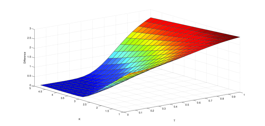
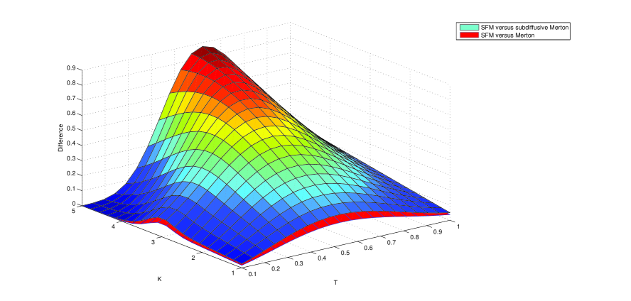
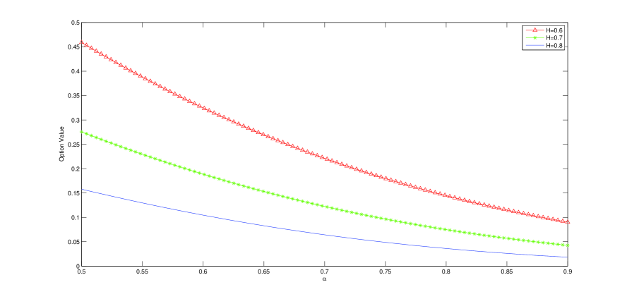
Figure 2. The European call option under S β F β M π πΉ π SFM . Where r 0 = 0.1 , Ξ± = 0.9 , H = 0.8 , Ο r = 0.3 , Ο s = 0.4 , S 0 = 3 , ΞΌ r = 0.2 , Ο = 0.2 formulae-sequence subscript π 0 0.1 formulae-sequence πΌ 0.9 formulae-sequence π» 0.8 formulae-sequence subscript π π 0.3 formulae-sequence subscript π π 0.4 formulae-sequence subscript π 0 3 formulae-sequence subscript π π 0.2 π 0.2 r_{0}=0.1,\alpha=0.9,H=0.8,\sigma_{r}=0.3,\sigma_{s}=0.4,S_{0}=3,\mu_{r}=0.2,\rho=0.2 .
Figure 3. The difference between the price of the European call option under S β F β M π πΉ π SFM , subdiffusive Merton and Merton models. Where r 0 = 0.1 , Ξ± = 0.9 , H = 0.8 , Ο r = 0.3 , Ο s = 0.4 , S 0 = 3 , ΞΌ r = 0.2 , t = 0 , Ο = 0.3 formulae-sequence subscript π 0 0.1 formulae-sequence πΌ 0.9 formulae-sequence π» 0.8 formulae-sequence subscript π π 0.3 formulae-sequence subscript π π 0.4 formulae-sequence subscript π 0 3 formulae-sequence subscript π π 0.2 formulae-sequence π‘ 0 π 0.3 r_{0}=0.1,\alpha=0.9,H=0.8,\sigma_{r}=0.3,\sigma_{s}=0.4,S_{0}=3,\mu_{r}=0.2,t=0,\rho=0.3 .
Figure 4. The European call option under S β F β M π πΉ π SFM . Where r 0 = 0.3 , Ο r = 0.1 , Ο s = 0.3 , S 0 = 4 , ΞΌ r = 0.2 , Ο = 0.2 , t = 0 , T = 0.2 formulae-sequence subscript π 0 0.3 formulae-sequence subscript π π 0.1 formulae-sequence subscript π π 0.3 formulae-sequence subscript π 0 4 formulae-sequence subscript π π 0.2 formulae-sequence π 0.2 formulae-sequence π‘ 0 π 0.2 r_{0}=0.3,\sigma_{r}=0.1,\sigma_{s}=0.3,S_{0}=4,\mu_{r}=0.2,\rho=0.2,t=0,T=0.2 .
We give three figures of the prices of European call options in the S β F β M π πΉ π SFM model for different parameters (see Figs. 2 , 3 and
4 ). From Equations (5.1 )-(5.7 ), it is easy to see that Ο i β m subscript π π π \sigma_{im} is just the implied volatility of the classical B β S π΅ π BS model.