A mixed discontinuous-continuous Galerkin time discretisation for Biot’s system

UWE KÖCHER1,†,∗ AND MARKUS BAUSE1,‡ 1 Helmut-Schmidt-University, University of the Federal Armed Forces Hamburg
Holstenhofweg 85, 22043 Hamburg, Germany
https://hsu-hh.de/mbm
koecher@hsu-hamburg.de ( corresponding author) bause@hsu-hamburg.de
Abstract

We study higher-order space-time variational discretisations for modeling complex processes in porous media that include fluid and structure interactions which are of fundamental importance in many engineering fields with applications in subsurface processes, battery-design and biomechanics. For the discretisation in time we deploy discontinuous Galerkin dG($r$) and continuous Galerkin cG($r$) discretisation families. Moreover we introduce a new coupled dG($r$)-cG($q$) mixed time discretisation and show numerically the stability advantages in the case of incompatible initial data under massively reduced computational costs. For the discretisation in space we use a mixed finite element method for the flow problem to ensure local mass conservation and a continuous Galerkin method for the mechanics. We consider solving sequentially the coupling of flow and mechanics with the fixed-stress iterative approach such that we can reuse our system solver and preconditioning technologies for the arising block system matrices from higher-order in time discretisations. Numerical experiments show firstly the undeniable advantages of discontinuous Galerkin time discretisations dG(0) and dG(1) over the continuous Galerkin time discretisation cG(1) in the case of incompatible initial data, secondly the advantages of the new coupled dG(1)-cG(1) in time approach in the case of incompatible initial data with massively reduced computational costs and better accuracy compared to the dG(1) time discretisation and thirdly the performance and efficiency differences of the dG(0), cG(1), dG(1) and the new dG(1)-cG(1) fixed-stress solver approaches for a sophisticated and physically relevant three-dimensional numerical example.

keywords:
Biot’s system, poroelasticity, space-time, discontinuous Galerkin dG($r$) time discretisation, continuous Galerkin cG($q$) time discretisation, coupled dG($r$)-cG($q$) Galerkin time discretisation, high-order time discretisations, fixed-stress operator splitting, stability comparision for incompatible data.
\heading

Uwe Köcher and Markus Bause

1 Introduction

Many engineering relevant fields involve interactions between flow and mechanical deformation throughout porous media. Important applications in environmental and petroleum engineering include subsurface carbon sequestration, compaction drive, hydraulic and thermal fracturing, and oil recovery for instance. Such problems belong to the family of thermo-hydro-mechanical (THM) problems in a more general sense. THM problems consist of coupled heat transfer (T), fluid flow (H) and matrix deformation (M). THM problems usually degenerate into their hydro-mechanical (HM) effects only for consolidation in fluid-saturated porous media processes, which are also known as poroelasticity problems. In reservoir engineering problems, for instance carbon sequestration problems, the characteristic time scale for the reservoir simulation is quite large compared to the intrinsic time scale of micro-mechanical behaviour such that dynamic effects are neglected. Dynamic poroelasticity models provide promising possibilities in battery-engineering for the design of next-generation batteries as well as in biomechanics for simulating modern vibration therapy for osteoporosis processes of trabeculae bones or estimating stress levels induced by tumour growth within the brain. The preceding vivid examples show the particular importance of the ability to simulate complex processes containing coupled flow and mechanical behaviour. However, mathematical modeling, the development of numerical approximation schemes and the development of efficient solver technology of such coupled processes remain challenging tasks for current research.

In this work, we study variational space-time numerical approximations of the coupled flow and deformation phenomena in its quasi-static limit for the mechanical deformation. Variational discretisation schemes for the temporal variable got a new spirit for their application to numerous fields of engineering relevance since sophisticated numerical solver technology was recently established but their origin can be traced back at least to 1969; cf. e.g. [32]. Using variational time methods offers some appreciable advantages such as the flexibility of the location of the degrees of freedom in time and the straightforward construction of higher-order approximations. In addition to that, an uniform variational method in space and time appears to be advantageous for stability and a priori error analyses of the discrete schemes; cf. e.g. [6]. In [7, 8] we studied the application of variational time discretisations for non-stationary diffusion problems and for the time domain elastic wave equation. Further, in [6] we presented error analysis for the existence and uniqueness of the semidiscrete and the fully discrete approximation for non-stationary diffusion problems. In [5] we presented briefly the application of a higher-order discontinuous in time variational scheme for Biot’s system of poroelasticity. In this work, we present details how the fully discrete systems in [5] were established and further study the numerical properties of the proposed schemes.

In [18] it is shown that the quasi-static Biot’s system can be obtained by taking the singular limit of the more general dynamic Biot-Allard’s system. Hereby, the Biot-Allard’s system is the result of a linearisation of dynamic fluid-structure interactions at the pore level. The further use of an homogenisation approach allows simulations at the macroscale level, i.e. the finite element level, with statically homogeneous material and flow properties. The resulting system of equations consist of an elastic wave equation for describing the dynamic behaviour of the mechanical deformation and a diffusion equation for describing the flow phenomena.

Further, solving the coupling of flow and mechanics sequentially by using operator splitting methods are studied in the literature and stability as well as convergence results were established; cf. [25, 11, 10, 23, 24, 22, 4].

General state of the art approaches exploit low-order finite difference methods for the time integration, such as the backward Euler scheme, the Crank-Nicolson scheme, $\theta$-schemes or BDF-schemes. Thus, the application of unconditionally stable higher order schemes for the time discretisation represents an innovation over previous works.

The novelity of this work is summarised by

  • $\bullet$

    the introduction of a new coupled dG($r$)-cG($q$) mixed time discretisation which is stable for incompatible initial data as the discontinuous Galerkin in time discretisation and having the reduced computational costs as the continuous Galerkin in time discretisation for $r=q\geq 1$,

  • $\bullet$

    the detailed study and derivation of fully-discrete algebraic systems of higher-order discontinuous and continuous Galerkin time discretisations combined with high-order multi-physics finite elements in space for Biot’s system of poroelasticitiy for the implementation of our efficient parallel-distributed solver suites with monolithic and iteratively coupled solvers [1] respectively [2], and

  • $\bullet$

    sophisticated three-dimensional numerical experiments of physically relevance to show the advantages, disadvantages and performance of the schemes and implemenations.

The further structure of this paper is organised as follows. Firstly we derive a mathematical model of the quasi-static Biot’s system from conservation and balance laws of the continuum problem in Sec. 2. Then we present the fixed-stress iterative approach for decoupling the flow and the mechanical subproblems for the infinite-dimensional space-time problem in Sec. 3. Furthermore we study in detail the application of variational space-time discretisations on the elliptic-mixed partial differential equation (PDE) system in Sec. 4. For the discretisation in time we apply members of the families of discontinuous and continuous in time Galerkin methods and further introduce a new coupled dG($r$)-cG($q$) mixed time discretisation in Sec. 4.6. For the discretisation in space we use a mixed finite element method (MFEM) for the flow problem and a finite element method for the mechanical problem. Thereby, the implementation within a distributed-parallel software of the applied space-time discretisation allows the solution of the presented sequential implicit splitting approach. Finally we study the stability and convergence properties of the presented schemes with some numerical experiments in Sec. 5 and summarise this work in Sec. 6.

2 Mathematical Model: Quasi-static Biot’s system

Throughout this paper we assume an isothermal single-phase flow, small mechanical deformations, an isotropic geomechanical material and stress-independence of flow properties; cf. [23, 24]. The further presentation is done in a dimensionless way, i.e. precisely we let the dimension $d\in\{2,3\}$ of the spatial domain $\Omega\subset\mathbb{R}^{d}$. The physical model is based on poroelasticity and poroelastoplasticity theories; cf. [26, 30]. The governing equations for coupled flow and geomechanics come from the mass conservation law and linear-momentum balance. Under the quasi-static assumption, the governing equation for mechanical deformation can be expressed by the elliptic partial differential equation

$$-\operatorname{div}\boldsymbol{\sigma}=\rho_{b}\boldsymbol{g}$$ (2.1)

where $\operatorname{div}(\cdot)$ is the divergence operator, $\boldsymbol{\sigma}$ is the Cauchy total stress tensor, $\rho_{b}=\phi\rho_{f}+(1-\phi)\rho_{s}$ is the time independent bulk density, $\phi$, with $0<\phi<1$, is the porosity, $\rho_{f}$ is the fluid phase mass density, $\rho_{s}$ is the solid phase mass density and $\boldsymbol{g}$ is some generalised volume force acting on the solid and the fluid like gravity. The porosity $\phi$ is defined as the ratio of the pore volume to the bulk volume in the deformed configuration. Under the assumption of slightly compressible fluid, the density $\rho_{f}$ is a positive constant. The solid matrix media is allowed to be heterogeneous such that the solid phase mass density $\rho_{s}$ and the $\phi$ may vary within the spatial domain. Thereby, the quantities $\rho_{s}$ and $\phi$ are restricted in a way such that they are piecewise constant and uniformly bounded from below and above as given by

$$0<\rho_{s}^{0}\leq\rho_{s}\leq\rho_{s}^{*}<\infty\quad\text{and}\quad 0<\phi^{0}\leq\phi\leq\phi^{*}<1\,.$$

The mechanical behaviour of the porous medium is specified by a stress-strain relationship. We let $\boldsymbol{\epsilon}(\boldsymbol{u})$ the linearised strain tensor applied on the displacement $\boldsymbol{u}$, which is defined component-wise as

$$\epsilon_{{\color[rgb]{0,0,1}\definecolor[named]{pgfstrokecolor}{rgb}{0,0,1}{i}}{\color[rgb]{0,0,1}\definecolor[named]{pgfstrokecolor}{rgb}{0,0,1}{j}}}(\boldsymbol{u})=\frac{1}{2}\bigg{(}\frac{\partial u_{{\color[rgb]{0,0,1}\definecolor[named]{pgfstrokecolor}{rgb}{0,0,1}{i}}}}{\partial x_{{\color[rgb]{0,0,1}\definecolor[named]{pgfstrokecolor}{rgb}{0,0,1}{j}}}}+\frac{\partial u_{{\color[rgb]{0,0,1}\definecolor[named]{pgfstrokecolor}{rgb}{0,0,1}{j}}}}{\partial x_{{\color[rgb]{0,0,1}\definecolor[named]{pgfstrokecolor}{rgb}{0,0,1}{i}}}}\bigg{)}\,,$$

with $1\leq{\color[rgb]{0,0,1}\definecolor[named]{pgfstrokecolor}{rgb}{0,0,1}{i}},{\color[rgb]{0,0,1}\definecolor[named]{pgfstrokecolor}{rgb}{0,0,1}{j}}\leq d$. The generalised Hooke’s law is given by

$$\boldsymbol{\sigma}^{\textnormal{eff}}(\boldsymbol{u})=\boldsymbol{C}\,\boldsymbol{\epsilon}(\boldsymbol{u})\,,\quad\sigma^{\textnormal{eff}}_{{\color[rgb]{0,0,1}\definecolor[named]{pgfstrokecolor}{rgb}{0,0,1}{i}}{\color[rgb]{0,0,1}\definecolor[named]{pgfstrokecolor}{rgb}{0,0,1}{j}}}=c_{{\color[rgb]{0,0,1}\definecolor[named]{pgfstrokecolor}{rgb}{0,0,1}{i}}{\color[rgb]{0,0,1}\definecolor[named]{pgfstrokecolor}{rgb}{0,0,1}{j}}{\color[rgb]{0,0,1}\definecolor[named]{pgfstrokecolor}{rgb}{0,0,1}{k}}{\color[rgb]{0,0,1}\definecolor[named]{pgfstrokecolor}{rgb}{0,0,1}{l}}}\,\epsilon_{{\color[rgb]{0,0,1}\definecolor[named]{pgfstrokecolor}{rgb}{0,0,1}{k}}{\color[rgb]{0,0,1}\definecolor[named]{pgfstrokecolor}{rgb}{0,0,1}{l}}}(\boldsymbol{u})\,,$$

with $1\leq{\color[rgb]{0,0,1}\definecolor[named]{pgfstrokecolor}{rgb}{0,0,1}{i}},{\color[rgb]{0,0,1}\definecolor[named]{pgfstrokecolor}{rgb}{0,0,1}{j}},{\color[rgb]{0,0,1}\definecolor[named]{pgfstrokecolor}{rgb}{0,0,1}{k}},{\color[rgb]{0,0,1}\definecolor[named]{pgfstrokecolor}{rgb}{0,0,1}{l}}\leq d$, where the summation over repeated indicies is implied, this notation is known as Einstein summation convention, and $\boldsymbol{C}$ is a piecewise constant rank-4 elasticity tensor of the drained soil, also known as Gassman’s tensor. For isotropic material $\boldsymbol{C}$ is given by

$$c_{{\color[rgb]{0,0,1}\definecolor[named]{pgfstrokecolor}{rgb}{0,0,1}{i}}{\color[rgb]{0,0,1}\definecolor[named]{pgfstrokecolor}{rgb}{0,0,1}{j}}{\color[rgb]{0,0,1}\definecolor[named]{pgfstrokecolor}{rgb}{0,0,1}{k}}{\color[rgb]{0,0,1}\definecolor[named]{pgfstrokecolor}{rgb}{0,0,1}{l}}}=\lambda\,\delta_{{\color[rgb]{0,0,1}\definecolor[named]{pgfstrokecolor}{rgb}{0,0,1}{i}}{\color[rgb]{0,0,1}\definecolor[named]{pgfstrokecolor}{rgb}{0,0,1}{j}}}\delta_{{\color[rgb]{0,0,1}\definecolor[named]{pgfstrokecolor}{rgb}{0,0,1}{k}}{\color[rgb]{0,0,1}\definecolor[named]{pgfstrokecolor}{rgb}{0,0,1}{l}}}+\mu\,(\delta_{{\color[rgb]{0,0,1}\definecolor[named]{pgfstrokecolor}{rgb}{0,0,1}{i}}{\color[rgb]{0,0,1}\definecolor[named]{pgfstrokecolor}{rgb}{0,0,1}{k}}}\delta_{{\color[rgb]{0,0,1}\definecolor[named]{pgfstrokecolor}{rgb}{0,0,1}{j}}{\color[rgb]{0,0,1}\definecolor[named]{pgfstrokecolor}{rgb}{0,0,1}{l}}}+\delta_{{\color[rgb]{0,0,1}\definecolor[named]{pgfstrokecolor}{rgb}{0,0,1}{i}}{\color[rgb]{0,0,1}\definecolor[named]{pgfstrokecolor}{rgb}{0,0,1}{l}}}\delta_{{\color[rgb]{0,0,1}\definecolor[named]{pgfstrokecolor}{rgb}{0,0,1}{j}}{\color[rgb]{0,0,1}\definecolor[named]{pgfstrokecolor}{rgb}{0,0,1}{k}}})\,,$$

where $\delta_{{\color[rgb]{0,0,1}\definecolor[named]{pgfstrokecolor}{rgb}{0,0,1}{i}}{\color[rgb]{0,0,1}\definecolor[named]{pgfstrokecolor}{rgb}{0,0,1}{j}}}$ denotes the Kronecker symbol, i.e. $\delta_{{\color[rgb]{0,0,1}\definecolor[named]{pgfstrokecolor}{rgb}{0,0,1}{i}}{\color[rgb]{0,0,1}\definecolor[named]{pgfstrokecolor}{rgb}{0,0,1}{j}}}=1$ if ${\color[rgb]{0,0,1}\definecolor[named]{pgfstrokecolor}{rgb}{0,0,1}{i}}={\color[rgb]{0,0,1}\definecolor[named]{pgfstrokecolor}{rgb}{0,0,1}{j}}$ and zero otherwise, and where $\lambda$ and $\mu$ are the Lamé parameters. These parameters can be expressed in terms of Young’s $E$ modulus and Poisson’s ratio $\nu$ as $\lambda=E\nu((1-2\nu)(1+\nu))^{-1}$ and $\mu=E(2(1+\nu))^{-1}$. In addition to this, Lame’s second parameter $\mu$ denotes the shear modulus $G$. Changes in the total stress and fluid pressure are related to changes in strain and fluid content by Biot’s theory; cf. [26, 27, 30]. We assume further that $\boldsymbol{E}:\boldsymbol{C}\boldsymbol{E}\geq\varepsilon\,|\boldsymbol{E}|^{2}+K_{\textnormal{dr}}\,(\operatorname{tr}\boldsymbol{E})^{2}$, $\varepsilon\geq 0$, is satisfied for any symmetric rank-2 tensor $\boldsymbol{E}$ and the bulk modulus $K_{\textnormal{dr}}$ of the drained soil. From [30], the poroelasticity equations for the Cauchy total stress tensor $\boldsymbol{\sigma}$ and the fluid mass $m$ per bulk volume have the following form:

$$\boldsymbol{\sigma}(\boldsymbol{u},p):=\boldsymbol{\sigma}_{0}+\boldsymbol{C}\,\boldsymbol{\epsilon}(\boldsymbol{u}-\boldsymbol{u}_{0})-\alpha\,(p-p_{0})\boldsymbol{1}\,,$$
$$m(\boldsymbol{u},p):=m_{0}+\rho_{f,0}\,\alpha\,\epsilon_{v}(\boldsymbol{u}-\boldsymbol{u}_{0})+\rho_{f,0}\,M^{-1}\,(p-p_{0})\,,$$ (2.2)

where $\boldsymbol{\sigma}_{0}$ is the reference state of the Cauchy total stress tensor, $\boldsymbol{u}_{0}$ is the reference state of the displacement vector field, $\alpha$ is the Biot’s coefficient, $p$ is the fluid pressure, $p_{0}$ is the reference state of the fluid pressure, $\boldsymbol{1}$ is the rank-2 identity tensor, $m_{0}$ is the reference state of the fluid mass per bulk volume, $\rho_{f,0}$ is the reference state of the fluid phase mass density, $\epsilon_{v}(\boldsymbol{u})=\operatorname{div}(\boldsymbol{u})$ is the volumetric strain of the displacement $\boldsymbol{u}$, and $M$ is the Biot’s modulus. The storage coefficient of a reservoir is defined as $c_{0}:=M^{-1}$. Biot studies in his original work [26] the relation of the scalar-valued model-coupling parameters $M$ and $\alpha$ to certain physical quantities under the assumption of an incompressible fluid that may contain air bubbles. Nowadays, the assumption of a slightly compressible fluid is generally taken, which is similar to the assumptions of Biot in the sense that the drained soil is not completely saturated due to microscopic inclusions of air bubbles. Following further [29, 30], we have the micromechanical relations

$$M^{-1}=\phi\,c_{f}+K_{s}^{-1}(\alpha-\phi)\,,\quad\textnormal{with}\quad c_{f}=K_{f}^{-1}\,,\quad\textnormal{and}\quad\alpha=1-K_{s}^{-1}K_{\textnormal{dr}}\,,$$ (2.3)

where $c_{f}$ is the fluid compressibility, $K_{f}$ is the bulk modulus of the fluid, $K_{s}$ is the bulk modulus of the solid grain, and $K_{\textnormal{dr}}$ is the drained bulk modulus. The most recent and ongoing research is on re-identifying the model-coupling parameters $M$ and $\alpha$ as rank-2 tensor-valued quantities derived by homogenisation techniques and verified with experimental data. The strain and stress tensors are decomposed in terms of their volumetric and deviatoric parts as given by

$$\boldsymbol{\epsilon}(\boldsymbol{u})=\frac{1}{3}\epsilon_{v}(\boldsymbol{u})\boldsymbol{1}+\boldsymbol{e}(\boldsymbol{u})\,,\quad\textnormal{with}\quad\epsilon_{v}(\boldsymbol{u})=\operatorname{tr}\boldsymbol{\epsilon}(\boldsymbol{u})=\operatorname{div}\boldsymbol{u}\,,\quad\textnormal{and}$$
$$\boldsymbol{\sigma}=\sigma_{v}\boldsymbol{1}+\boldsymbol{s}\,,\quad\textnormal{with}\quad\sigma_{v}=\frac{1}{3}\operatorname{tr}\boldsymbol{\sigma}\,,$$

respectively, where $\epsilon_{v}(\boldsymbol{u})$ is the volumetric strain, i.e. the trace of the strain tensor, $\boldsymbol{e}$ is the deviatoric part of the strain tensor, $\sigma_{v}$ is the volumetric (mean) total stress and $\boldsymbol{s}$ is the deviatoric total stress tensor. We use the convention of positive tensile and compression stresses. The relationship between the volumetric stress and strain is given by

$$\sigma_{v}:=\sigma_{v}(\boldsymbol{u},p)=\displaystyle\sigma_{v,0}+K_{\textnormal{dr}}\,\epsilon_{v}(\boldsymbol{u}-\boldsymbol{u}_{0})-\alpha(p-p_{0})\,.$$ (2.4)

We further derive Biot’s model of poroelasticity under quasi-static conditions in which the stress evolution and the fluid acceleration due to dynamical mechanical acceleration terms $\partial_{tt}\boldsymbol{u}$ can be neglected since the assumptions of $|\partial_{t}\nabla p|\gg|\partial_{tt}\boldsymbol{u}|$ and $|\partial_{tt}\boldsymbol{u}|=\mathcal{O}(0)$ hold for the time scale of physical interest. We assume that the pores are small enough such that the flow through the porous medium is laminar. The fluid velocity $\boldsymbol{q}$ relative to the solid phase is given by Darcy’s law

$$\boldsymbol{q}:=\displaystyle-\frac{1}{\eta}\boldsymbol{K}(\nabla p-\rho_{f}\boldsymbol{g})\,,$$ (2.5)

where $\eta$ is the fluid viscosity and $\boldsymbol{K}$ is the permeability tensor. The fluid viscosity is restricted to be piecewise constant and the permeability tensor field $\boldsymbol{K}$ is supposed to be a piecewise constant and being a symmetric and uniformly positive definite matrix. For simplicity we assume that the fluid viscosity and permeability do not depend on the history since otherwise memory terms involving fractional time-derivatives would appear in the model; cf. [18]. The fluid mass conservation law under the assumption of small deformation is given by

$$\partial_{t}m(\boldsymbol{u},p)+\nabla\cdot(\rho_{f,0}\,\boldsymbol{q})=\rho_{f,0}\,f\,,$$ (2.6)

where $(\rho_{f,0}\,\boldsymbol{q})$ denote the fluid mass flux, i.e. the fluid mass flow rate per unit area and time, and $f$ denote a volumetric source term. More precisely, $f$ can be physically interpreted as a volumetric fluid producing source or fluid absorbing sink term. Additional convection terms and reaction terms are neglected for simplicity.

The fully coupled problem, which is a parabolic partial differential equation coupled to the quasi-static mechanical problem of Eq. (2.1), is derived by combining the fluid mass conservation law given by Eq. (2.6) with the mass balance law from Eq. (2.2) and the relationship from Eq. (2.4) as follows

$$\displaystyle\frac{\alpha}{K_{\textnormal{dr}}}\partial_{t}\sigma_{v}(\boldsymbol{u},p)+\bigg{(}\frac{1}{M}+\frac{\alpha^{2}}{K_{\textnormal{dr}}}\bigg{)}\partial_{t}p+\operatorname{div}\boldsymbol{q}=f\,.$$

In the sequel of this work, we use standard notation for function spaces and their respective norms and define the function spaces $W:=L^{2}(\Omega)$ as function space of square integrable functions, $\boldsymbol{V}:=\boldsymbol{H}(\operatorname{div};\Omega)=\{\boldsymbol{v}\in L^{2}(\Omega)^{d}\,|\,\nabla\cdot\boldsymbol{v}\in L^{2}(\Omega)\}$ as function space of square integrable vector-valued functions with square integrable divergence, $\boldsymbol{V}_{0}:=\{\boldsymbol{v}\in\boldsymbol{H}(\operatorname{div};\Omega)\,|\,(\boldsymbol{v}\cdot\boldsymbol{n})|_{\Gamma_{q}}=0\}$ fulfilling additionally homogeneous boundary conditions, and $\boldsymbol{H}_{0}:=H^{1}_{0}(\Gamma_{\boldsymbol{u}};\Omega)^{d}$ as function space of vector-valued componentwise $H^{1}(\Omega)$ functions with vanishing trace on $\Gamma_{\boldsymbol{u}}$ for brevity. Thereby, we denote by $H^{m}(\Omega)$ the Sobolev space of $L^{2}(\Omega)$ functions with derivatives up to order $m$ in $L^{2}(\Omega)$. We let $(\cdot,\cdot)$ denote the respective $L^{2}(\Omega)$-, $L^{2}(\Omega)^{d}$- or $L^{2}(\Omega)^{d\times d}$-inner product. Let $X$ a reflexive Banach space. We introduce the following Bochner spaces with values in a Banach space $X$ as

$$\begin{array}[]{rcl}C(\widebar{I};X)&=&\{v:[0,T]\to X\,|\,v\,\text{is continuous on $[0,T]$ with respect to $t$.}\}\,,\\[6.45831pt] L^{2}(I;X)&=&\bigg{\{}v:(0,T)\to X\,\bigg{|}\,\Big{(}\displaystyle\int_{I}\|v(t)\|_{X}^{2}\,\mathrm{d}t\Big{)}^{0.5}<\infty\bigg{\}}\,,\\[12.91663pt] H^{1}(I;X)&=&\{v:L^{2}(I;X)\,|\,\partial_{t}v\in L^{2}(I;X)\}\,.\end{array}$$

Quasi-static Biot’s system. The fully coupled partial differential equations system in strong form, which is precisely a coupled hydro-mechanical (HM) problem for the approximation of the displacement, flux and pressure variables, reads as: Find $\boldsymbol{u}$, $\boldsymbol{q}$ and $p$ in either $d=2$ or $d=3$ space dimensions from

$$\begin{array}[]{rcl@{\quad}l}\displaystyle-\nabla\cdot\Big{(}\boldsymbol{\sigma}_{0}+\boldsymbol{C}\,\boldsymbol{\epsilon}(\boldsymbol{u}-\boldsymbol{u}_{0})-\alpha\,(p-p_{0})\boldsymbol{1}\Big{)}&=&\rho_{b}\,\boldsymbol{g}&\textnormal{in}\quad\Omega\times I\,,\\[12.91663pt] \displaystyle\eta\,\boldsymbol{K}^{-1}\boldsymbol{q}+\nabla p&=&\rho_{f}\,\boldsymbol{g}&\textnormal{in}\quad\Omega\times I\,,\\[6.45831pt] \displaystyle-\frac{\alpha}{K_{\textnormal{dr}}}\partial_{t}\sigma_{v}(\boldsymbol{u},p)-\operatorname{div}\boldsymbol{q}-\bigg{(}\frac{1}{M}+\frac{\alpha^{2}}{K_{\textnormal{dr}}}\bigg{)}\partial_{t}p&=&-f&\textnormal{in}\quad\Omega\times I\,,\\[12.91663pt] \end{array}$$ (2.7)

with the relationship of the volumetric stress and strain

$$\sigma_{v}(\boldsymbol{u},p)=\displaystyle\sigma_{v,0}+K_{\textnormal{dr}}\,\epsilon_{v}(\boldsymbol{u}-\boldsymbol{u}_{0})-\alpha\,(p-p_{0})\,,$$

and satisfying the initial conditions

$$\begin{array}[]{rcl@{\quad}l @{\quad} rcl@{\quad}l}\boldsymbol{\sigma}(\boldsymbol{x},0)&=&\boldsymbol{\sigma}_{0}&\textnormal{in}\quad\Omega\times\{0\}\,,&\boldsymbol{u}(\boldsymbol{x},0)&=&\boldsymbol{u}_{0}&\textnormal{in}\quad\Omega\times\{0\}\,,\\[6.45831pt] p(\boldsymbol{x},0)&=&p_{0}&\textnormal{in}\quad\Omega\times\{0\}\,,\end{array}$$

and the boundary conditions

$$\begin{array}[]{rcl@{\quad}l @{\quad} rcl@{\quad}l}\boldsymbol{u}&=&\boldsymbol{u}_{D}&\textnormal{on}\quad\Gamma_{\boldsymbol{u}}\times I\,,&\boldsymbol{\sigma}\,\boldsymbol{n}&=&\boldsymbol{t}_{N}&\textnormal{on}\quad\Gamma_{\boldsymbol{t}}\times I\,,\\[6.45831pt] p&=&p_{D}&\textnormal{on}\quad\Gamma_{p}\times I\,,&\boldsymbol{q}\cdot\boldsymbol{n}&=&q_{v}&\textnormal{on}\quad\Gamma_{q}\times I\,.\end{array}$$

The existence and uniqueness of solutions as well as regularity theory for Biot’s system of poroelasticity (2.7) is presented in a Hilbert space setting in [16]. The the well-posedness is further shown in [17] for a wider class of diffusion problems in poro-plastic media. In [18, Thm. 3] the existence and uniqueness of solutions are proofed by applying modern model homogenisation techniques which we will further briefly summarise. Under periodic boundary conditions for $\boldsymbol{u}$ and $p$ with period $L$, for smooth $L$-periodic functions $p_{0}$, $f$ and $\boldsymbol{\sigma}_{0}$ and assumptions on the media parameters for flow and mechanics, Biot’s system from Eq. (2.7) admits an unique variational solution

$$\{\boldsymbol{u},p\}\in H_{\text{per},0}^{1}((0,T)\times\Omega^{L})^{d}\cap H^{2}(0,T;L^{2}(\Omega^{L}))^{d}\times H_{0}^{1}(0,T;L^{2}(\Omega^{L}))\cap L^{2}(0,T;H_{\text{per}}^{1}(\Omega^{L}))\,,$$

in the poroelastic cube $\Omega^{L}$, where the function spaces with the subscript “per” must hold periodic boundary conditions in the spatial domain and the function spaces with the subscript “00” must hold homogeneous initial conditions in the temporal domain of the tensor product space-time cube $Q=(0,T)\times\Omega^{L}$. Further, additional high-order smoothness in time, i.e.

$$\{\boldsymbol{u},p\}\in H^{k}(0,T;H_{\text{per}}^{1}(\Omega^{L}))^{d+1}\,,\quad\displaystyle\int_{\Omega^{L}}\boldsymbol{u}(\boldsymbol{x},t)\,\mathrm{d}\boldsymbol{x}=0\quad\text{for a.e. }t\in(0,T)\,,\quad\text{for all }k\in\mathbb{N}\,,$$

of the quasi-static Biot’s system two-field solution $\{\boldsymbol{u},p\}$ was established in [18, Lem. 3] under the additional assumption of $\boldsymbol{g}\in C^{\infty}_{0}(\mathbb{R}^{+};L^{2}(\Omega^{L})^{d})$. For existence and uniqueness of solutions involving more general boundary conditions we refer to [12] and the given references therein. Following [18], the quasi-static Biot’s system is valid for almost every $\boldsymbol{x}\in\Omega^{L}\subset\Omega$ in the poroelastic cube $\Omega^{L}=(0,L)^{d}$, $d=2,3$, and for almost every $t\in I=(0,T)$, $T<\infty$. Additionally, assume the partition of the poroelastic cube $\Omega^{L}=\Omega_{s}\cup\Omega_{f}$, $\Omega_{s}\neq\emptyset$, $\Omega_{f}\neq\emptyset$, into its deformable solid skeleton part $\Omega_{s}$ and its pore part $\Omega_{f}$ containing the fluid on the microscale. $\Omega_{f}$ is supposed to be an open periodic set with positive measure and a smooth boundary; cf. for details [18, 31]. Additionally, the pore space $\Omega_{f}$ is assumed to be completely filled by a fluid at all times such that the fluid and solid phases are fully connected. We remark that the assumptions taken on the microscale are crucial for the development of a macroscale model by homogenisation techniques which is further used as our simulation scale. For well-posedness of the problem, we assume the partition of the boundary $\partial\Omega=\Gamma_{\boldsymbol{u}}\cup\Gamma_{\boldsymbol{t}}$, with $\Gamma_{\boldsymbol{u}}\cap\Gamma_{\boldsymbol{t}}=\emptyset$, for the mechanics and the independent partition of the boundary $\partial\Omega=\Gamma_{p}\cup\Gamma_{q}$, with $\Gamma_{p}\cap\Gamma_{q}=\emptyset$ for the flow problem. We remark that the boundary conditions for the mechanical problem may be mixed componentwise for physically relevant problems and inhomogeneous Dirichlet boundary values $\boldsymbol{u}_{D}$ can be incorporated in a standard way. The initial state of strains $\boldsymbol{\epsilon}(\boldsymbol{u}(\cdot,0)-\boldsymbol{u}_{0})$ is, by definition, homogeneous in the given model above. The proper initialisation of the geomechanical problem is non-trivial and such, we refer to the literature; cf. e.g. [28]. Being more precisely, the initial stress $\boldsymbol{\sigma}_{0}$ should satisfy the mechanical equilibrium, i.e. $-\nabla\cdot\boldsymbol{\sigma}_{0}=\rho_{b}\,\boldsymbol{g}(\cdot,0)$, and reflect the history of stress paths in the formation of the reservoir in order to avoid stability issues.

Weak formulation for quasi-static Biot’s system. The fully coupled partial differential equations system in weak form reads as: Find $\boldsymbol{u}\in L^{2}(I;H^{1}_{0}(\Gamma_{\boldsymbol{u}};\Omega)^{d})\cap H^{1}(I;H^{1}(\Omega)^{d})$, $\boldsymbol{q}\in L^{2}(I;\boldsymbol{V}_{0})$ and $p\in H^{1}(I;L^{2}(\Omega))$ in either $d=2$ or $d=3$ space dimensions from

$$\begin{array}[]{l}\displaystyle\int_{I}\int_{\Omega}\boldsymbol{\epsilon}(\boldsymbol{z}):\Big{(}\boldsymbol{\sigma}_{0}+\boldsymbol{C}\,\boldsymbol{\epsilon}(\boldsymbol{u}-\boldsymbol{u}_{0})-\alpha\,(p-p_{0})\boldsymbol{1}\Big{)}\,\mathrm{d}\boldsymbol{x}\,\mathrm{d}t=\\[12.91663pt] \displaystyle\quad\int_{I}\int_{\Omega}\boldsymbol{z}\cdot\rho_{b}\,\boldsymbol{g}\,\mathrm{d}\boldsymbol{x}\,\mathrm{d}t+\int_{I}\int_{\Gamma_{\boldsymbol{t}}}\boldsymbol{z}\cdot\boldsymbol{t}_{N}\,\mathrm{d}\boldsymbol{x}\,\mathrm{d}t\,,\quad\forall\boldsymbol{z}\in L^{2}(I;H^{1}_{0}(\Gamma_{\boldsymbol{u}};\Omega)^{d})\,,\\[19.37494pt] \displaystyle\int_{I}\int_{\Omega}\boldsymbol{v}\cdot\eta\,\boldsymbol{K}^{-1}\boldsymbol{q}\,\mathrm{d}\boldsymbol{x}\,\mathrm{d}t-\int_{I}\int_{\Omega}(\nabla\cdot\boldsymbol{v})\,p\,\mathrm{d}\boldsymbol{x}\,\mathrm{d}t=\\[12.91663pt] \displaystyle\quad\int_{I}\int_{\Omega}\boldsymbol{v}\cdot\rho_{f}\,\boldsymbol{g}\,\mathrm{d}\boldsymbol{x}\,\mathrm{d}t-\int_{I}\int_{\Gamma_{p}}(\boldsymbol{v}\cdot\boldsymbol{n})\,p_{D}\,\mathrm{d}\boldsymbol{x}\,\mathrm{d}t\,,\quad\forall\boldsymbol{v}\in L^{2}(I;\boldsymbol{V}_{0})\,,\\[19.37494pt] \displaystyle-\int_{I}\int_{\Omega}w\,\operatorname{div}\boldsymbol{q}\,\mathrm{d}\boldsymbol{x}\,\mathrm{d}t-\int_{I}\int_{\Omega}w\,\bigg{(}\frac{1}{M}+\frac{\alpha^{2}}{K_{\textnormal{dr}}}\bigg{)}\partial_{t}p\,\mathrm{d}\boldsymbol{x}\,\mathrm{d}t\\[12.91663pt] \displaystyle\quad-\int_{I}\int_{\Omega}w\,\frac{\alpha}{K_{\textnormal{dr}}}\partial_{t}\sigma_{v}(\boldsymbol{u},p)\,\mathrm{d}\boldsymbol{x}\,\mathrm{d}t=-\int_{I}\int_{\Omega}w\,f\,\mathrm{d}\boldsymbol{x}\,\mathrm{d}t\,,\,\,\forall w\in L^{2}(I;L^{2}(\Omega))\,,\end{array}$$ (2.8)

with the relationship of the volumetric stress and strain

$$\sigma_{v}(\boldsymbol{u},p)=\displaystyle\sigma_{v,0}+K_{\textnormal{dr}}\,\epsilon_{v}(\boldsymbol{u}-\boldsymbol{u}_{0})-\alpha\,(p-p_{0})\,,$$

and satisfying the initial conditions

$$\begin{array}[]{rcl@{\quad}l @{\quad} rcl@{\quad}l}\boldsymbol{\sigma}(\boldsymbol{x},0)&=&\boldsymbol{\sigma}_{0}&\textnormal{in}\quad\Omega\times\{0\}\,,&\boldsymbol{u}(\boldsymbol{x},0)&=&\boldsymbol{u}_{0}&\textnormal{in}\quad\Omega\times\{0\}\,,\\[6.45831pt] p(\boldsymbol{x},0)&=&p_{0}&\textnormal{in}\quad\Omega\times\{0\}\,.\end{array}$$

3 Operator splitting for the continuum problem

In this section we present an operator splitting method for the given continuum problem, i.e. the quasi-static Biot’s system derived in Sec. 2, which is of the fixed-stress iterative approach type. The goal is to decouple the mechanical problem and the flow problem. With that, it is possible to solve the two subproblems sequentially within an iterative scheme. The computational overhead for the outer iteration can be resolved since optimised and high-performance solvers can be used for each subproblem. For low-order time discretisations the first half-step is sometimes denoted as a half-time step but for higher order time discretisations, which have at least two sets of unknown degrees of freedom in time per variable, such an interpretation does not hold. Thus, we do not use the notation of a half-time step.

The fixed-stress operator splitting method is already well studied and compared against other splitting methods for standard time discretisations in the recent research work of [21, 20, 22, 24]. It is motivated by fixing the ratio of the volumetric stress $\delta\partial_{t}\sigma_{v}(\boldsymbol{u},p)=0$ during the first half of each fixed-point iteration step in which the flow (H) problem is solved independently, and then the mechanical (M) problem is solved independently with the updated values and the prescribed pressure $p$ in the second half of each iteration step.

Let ‘${\color[rgb]{1,0,0}\definecolor[named]{pgfstrokecolor}{rgb}{1,0,0}{s}}$’ denote the fixed-point iteration index. The ratio of the temporal change of the volumetric stress $\delta\partial_{t}\sigma_{v}(\boldsymbol{u},p)=\partial_{t}\sigma_{v}^{{\color[rgb]{1,0,0}\definecolor[named]{pgfstrokecolor}{rgb}{1,0,0}{s}}+0.5}-\partial_{t}\sigma_{v}^{{\color[rgb]{1,0,0}\definecolor[named]{pgfstrokecolor}{rgb}{1,0,0}{s}}}=0$ is constrained to vanish in the first half-step. By using the relation from Eq. (2.4) we find that

$$\partial_{t}\sigma_{v}^{{\color[rgb]{1,0,0}\definecolor[named]{pgfstrokecolor}{rgb}{1,0,0}{s}}+0.5}\stackrel{{\scriptstyle!}}{{=}}\partial_{t}\sigma_{v}^{{\color[rgb]{1,0,0}\definecolor[named]{pgfstrokecolor}{rgb}{1,0,0}{s}}}=K_{\textnormal{dr}}^{*}\,\partial_{t}\epsilon_{v}(\boldsymbol{u}^{{\color[rgb]{1,0,0}\definecolor[named]{pgfstrokecolor}{rgb}{1,0,0}{s}}})-\alpha\,\partial_{t}p^{{\color[rgb]{1,0,0}\definecolor[named]{pgfstrokecolor}{rgb}{1,0,0}{s}}}$$

must be fulfilled. As a remark, we have here replaced the bulk modulus of the drained soil $K_{\textnormal{dr}}$ by some mathematically chosen $K_{\textnormal{dr}}^{*}>0$. The arbitrary choice of $K_{\textnormal{dr}}^{*}$ is studied in the literature for optimality in [19, 4, 21, 22], but the optimal value depend on various parameters as it is studied in [3]. Fluxes and pressures are prescribed with the values $\{\boldsymbol{q}^{{\color[rgb]{1,0,0}\definecolor[named]{pgfstrokecolor}{rgb}{1,0,0}{s}}+0.5},p^{{\color[rgb]{1,0,0}\definecolor[named]{pgfstrokecolor}{rgb}{1,0,0}{s}}+0.5}\}$ from the first half iteration step on the second half of each iteration step such that $\{\boldsymbol{q}^{{\color[rgb]{1,0,0}\definecolor[named]{pgfstrokecolor}{rgb}{1,0,0}{s}}+1},p^{{\color[rgb]{1,0,0}\definecolor[named]{pgfstrokecolor}{rgb}{1,0,0}{s}}+1}\}:=\{\boldsymbol{q}^{{\color[rgb]{1,0,0}\definecolor[named]{pgfstrokecolor}{rgb}{1,0,0}{s}}+0.5},p^{{\color[rgb]{1,0,0}\definecolor[named]{pgfstrokecolor}{rgb}{1,0,0}{s}}+0.5}\}$. The fixed-stress iterative approach for the continuum problem reads as: For ${\color[rgb]{1,0,0}\definecolor[named]{pgfstrokecolor}{rgb}{1,0,0}{s}}=0,\,\dots,$ until convergence do:

  1. (H):

    Find $\boldsymbol{q}^{{\color[rgb]{1,0,0}\definecolor[named]{pgfstrokecolor}{rgb}{1,0,0}{s}}+1}\in L^{2}(I;\boldsymbol{V}_{0})$ and $p^{{\color[rgb]{1,0,0}\definecolor[named]{pgfstrokecolor}{rgb}{1,0,0}{s}}+1}\in H^{1}(I;L^{2}(\Omega))$ from

    $$\begin{array}[]{@{\!\!\!\!}l@{\;}l}{}&\displaystyle\int_{I}(\boldsymbol{v},\eta\,\boldsymbol{K}^{-1}\boldsymbol{q}^{{\color[rgb]{1,0,0}\definecolor[named]{pgfstrokecolor}{rgb}{1,0,0}{s}}+1})\,\mathrm{d}t-\int_{I}(\nabla\cdot\boldsymbol{v},p^{{\color[rgb]{1,0,0}\definecolor[named]{pgfstrokecolor}{rgb}{1,0,0}{s}}+1})\,\mathrm{d}t=\\[12.91663pt] {}&\displaystyle\quad\int_{I}(\boldsymbol{v},\rho_{f}\,\boldsymbol{g})\,\mathrm{d}t-\int_{I}(\boldsymbol{v}\cdot\boldsymbol{n},p_{D})_{\Gamma_{p}}\,\mathrm{d}t\,,\quad\forall\boldsymbol{v}\in L^{2}(I;\boldsymbol{V}_{0})\,,\\[19.37494pt] -&\displaystyle\int_{I}(w,\operatorname{div}\boldsymbol{q}^{{\color[rgb]{1,0,0}\definecolor[named]{pgfstrokecolor}{rgb}{1,0,0}{s}}+1})\,\mathrm{d}t-\int_{I}\bigg{(}w,\bigg{(}\frac{1}{M}+\frac{\alpha^{2}}{K_{\textnormal{dr}}^{*}}\bigg{)}\partial_{t}p^{{\color[rgb]{1,0,0}\definecolor[named]{pgfstrokecolor}{rgb}{1,0,0}{s}}+1}\bigg{)}\,\mathrm{d}t=-\int_{I}(w,f)\,\mathrm{d}t\\[12.91663pt] {}&\displaystyle\quad+\int_{I}(w,\alpha\,\epsilon_{v}(\partial_{t}\boldsymbol{u}^{{\color[rgb]{1,0,0}\definecolor[named]{pgfstrokecolor}{rgb}{1,0,0}{s}}}))\,\mathrm{d}t-\int_{I}\bigg{(}w,\frac{\alpha^{2}}{K_{\textnormal{dr}}^{*}}\,\partial_{t}p^{{\color[rgb]{1,0,0}\definecolor[named]{pgfstrokecolor}{rgb}{1,0,0}{s}}}\bigg{)}\,\mathrm{d}t\,,\quad\forall w\in L^{2}(I;L^{2}(\Omega))\,,\end{array}$$ (3.1)

    satisfying the initial condition $p^{{\color[rgb]{1,0,0}\definecolor[named]{pgfstrokecolor}{rgb}{1,0,0}{s}}+1}(\cdot,0)=p_{0}$.

  2. (M):

    Find $\boldsymbol{u}^{{\color[rgb]{1,0,0}\definecolor[named]{pgfstrokecolor}{rgb}{1,0,0}{s}}+1}\in L^{2}(I;H^{1}_{0}(\Gamma_{\boldsymbol{u}};\Omega)^{d})\cap H^{1}(I;H^{1}(\Omega)^{d})$ from

    $$\begin{array}[]{l}\displaystyle\int_{I}\Big{(}\boldsymbol{\epsilon}(\boldsymbol{z}),\boldsymbol{\sigma}_{0}\Big{)}\,\mathrm{d}t+\int_{I}\Big{(}\boldsymbol{\epsilon}(\boldsymbol{z}),\boldsymbol{C}\,\boldsymbol{\epsilon}(\boldsymbol{u}^{{\color[rgb]{1,0,0}\definecolor[named]{pgfstrokecolor}{rgb}{1,0,0}{s}}+1}-\boldsymbol{u}_{0})\Big{)}\,\mathrm{d}t=\int_{I}\Big{(}\boldsymbol{\epsilon}(\boldsymbol{z}),\alpha\,(p^{{\color[rgb]{1,0,0}\definecolor[named]{pgfstrokecolor}{rgb}{1,0,0}{s}}+1}-p_{0})\boldsymbol{1}-\boldsymbol{\sigma}_{0}\Big{)}\,\mathrm{d}t\\[12.91663pt] \displaystyle\quad+\int_{I}(\boldsymbol{z},\rho_{b}\,\boldsymbol{g})\,\mathrm{d}t+\int_{I}(\boldsymbol{z},\boldsymbol{t}_{N})_{\Gamma_{\boldsymbol{t}}}\,\mathrm{d}t\,,\quad\forall\boldsymbol{z}\in L^{2}(I;H^{1}_{0}(\Gamma_{\boldsymbol{u}};\Omega)^{d})\,,\end{array}$$ (3.2)

    satisfying the initial condition $\boldsymbol{u}^{{\color[rgb]{1,0,0}\definecolor[named]{pgfstrokecolor}{rgb}{1,0,0}{s}}+1}(\cdot,0)=\boldsymbol{u}_{0}$.

We remark that the convergence in terms of a fixed-point iteration for the continuum problem means here $\{\boldsymbol{u}^{\star},\boldsymbol{q}^{\star},p^{\star}\}=\{\boldsymbol{u}^{{\color[rgb]{1,0,0}\definecolor[named]{pgfstrokecolor}{rgb}{1,0,0}{s}}+1},\boldsymbol{q}^{{\color[rgb]{1,0,0}\definecolor[named]{pgfstrokecolor}{rgb}{1,0,0}{s}}+1},p^{{\color[rgb]{1,0,0}\definecolor[named]{pgfstrokecolor}{rgb}{1,0,0}{s}}+1}\}=\{\boldsymbol{u}^{{\color[rgb]{1,0,0}\definecolor[named]{pgfstrokecolor}{rgb}{1,0,0}{s}}},\boldsymbol{q}^{{\color[rgb]{1,0,0}\definecolor[named]{pgfstrokecolor}{rgb}{1,0,0}{s}}},p^{{\color[rgb]{1,0,0}\definecolor[named]{pgfstrokecolor}{rgb}{1,0,0}{s}}}\}$ for almost every $(\boldsymbol{x},t)\in\Omega\times I$. Also we remark that the time discretisations of (H) and (M) must not necessarily be the same.

4 Variational space-time discretisation

In this section we present details of the applied variational space-time discretisations. For the discretisation in time we use a discontinuous Galerkin dG($r$) method with piecewise polynomials of order $r\geq 0$ in time and a continuous Galerkin cG($q$) method with piecewise polynomials of order $q\geq 1$ in time. For discontinuous Galerkin dG($r$) in time methods we use the same spaces for trial and test functions while we use precisely a (continuous) Petrov-Galerkin cG($q$) in time method with continuous trial functions and discontinuous test functions; cf. for details [8, 5, 7]. We are allowed to solve (efficient) time marching schemes instead of the global space-time scheme due to the discontinuous in time test function space.

The global time interval $I=(0,T)$ is decomposed as $\widebar{I}=\bigcup_{n=1}^{N}\widebar{I}_{n}$, $I_{n}=(t_{n-1},t_{n})$, $n=1,\dots,N$, with $0=:t_{0}<\cdots<t_{n}<\cdots<t_{N}:=T$. The time subinterval length of $I_{n}$ is $\tau_{n}=t_{n}-t_{n-1}$ and the global time discretisation parameter is defined as $\tau:=\max_{n=1,\dots,N}\tau_{n}$. The reference interval in time is defined as $\widehat{I}:=[0,1]$. The affine mapping $\mathcal{T}_{n}:\widehat{I}\to\widebar{I}_{n}$ and its inverse $\mathcal{T}_{n}^{-1}:\widebar{I}_{n}\to\widehat{I}$ are given by

$$\mathcal{T}_{n}(\widehat{I}):=\tau_{n}\widehat{t}+t_{n-1}\,,\quad\mathcal{T}_{n}^{-1}(t):=(t-t_{n-1})/\tau_{n}\,,\quad n=1,\dots,N\,.$$ (4.1)

For time-discrete globally discontinuous functions, we allow the left-hand side values $w(t_{n}^{-})$ to be different from the right-hand side values $w(t_{n}^{+})$. We let $\mathbb{P}_{r}(I_{n};X)$ denote the space of polynomials in time up to degree $r\geq 0$ on $I_{n}$ with values in a Banach space $X$. We introduce for some Banach space $X$ the discontinuous in time function space

$$\begin{array}[]{r@{\,}c@{\,}l@{\,}c@{\,}l}\mathcal{V}^{\textnormal{dG($r$)}}_{\tau}(X)&:=&\Big{\{}v\in L^{2}(I;X)&\Big{|}&v|_{I_{n}}\in\mathbb{P}_{r}(I_{n};X)\,,\,\,n=1,\dots,N\Big{\}}\,,\quad r\geq 0\,,\end{array}$$ (4.2)

and the continuous in time function space

$$\begin{array}[]{r@{\,}c@{\,}l@{\,}c@{\,}l}\mathcal{V}^{\textnormal{cG($q$)}}_{\tau}(X)&:=&\Big{\{}v\in C(\widebar{I};X)&\Big{|}&v|_{I_{n}}\in\mathbb{P}_{q}(\widebar{I}_{n};X)\,,\,\,n=1,\dots,N\Big{\}}\,,\quad q\geq 1\,.\end{array}$$ (4.3)

which are both discrete and finite dimensional in time. Functions $v_{\tau}$ of the discrete space $\mathcal{V}^{\textnormal{dG($r$)}}_{\tau}$, or $\mathcal{V}^{\textnormal{cG($q$)}}_{\tau}$, can be separated into their temporal and spatial parts as $v_{\tau}(\boldsymbol{x},t)=\widehat{v}(\boldsymbol{x})\cdot\widetilde{v}(t)$.

For the discretisation in space, we give the partition $\mathcal{T}_{h}$ of the domain $\Omega$ into some finite number of disjoint elements $K$, such that $\widebar{\Omega}=\bigcup_{K\in\mathcal{T}_{h}}\widebar{K}$. For simplicity, we choose the elements $K\in\mathcal{T}_{h}$ to be quadrilaterals ($d=2$) or hexahedrals ($d=3$). We assume that adjacent elements completely share their common edge or face. We denote by $h_{K}$ the diameter of the element $K$. The global space discretisation parameter $h$ is given by $h=\max_{K\in\mathcal{T}_{h}}h_{K}$. We allow the mesh to be anisotropic but non-degenerated. For the approximation of the function space $\boldsymbol{V}_{0}:=\{\boldsymbol{v}\in\boldsymbol{H}(\operatorname{div};\Omega)\,|\,(\boldsymbol{v}\cdot\boldsymbol{n})|_{\Gamma_{q}}=0\}$ we use the $\textnormal{RT}_{p-1}$ Raviart-Thomas-Nédélec finite element space such that the pressure $p_{h}$ is piecewise polynomial of order $(p-1)\geq 0$ on the reference cell and we use a continuous finite element space $\boldsymbol{Q}_{h}^{p}$, employing constraints on the degrees of freedom on homogeneous Dirichlet type boundary on $\Gamma_{\boldsymbol{u}}\times I$, for vector-valued functions on quadrilaterals or hexahedrals such that the displacement $\boldsymbol{u}_{h}$ is piecewise polynomial of order $p\geq 1$ on the reference cell; cf. [8].

Furthermore we use the notation of ζn,ι(t)r(I¯n;)subscript𝜁𝑛𝜄𝑡subscript𝑟subscript¯𝐼𝑛\zeta_{n,{\color[rgb]{0,1,0}\definecolor[named]{pgfstrokecolor}{rgb}{0,1,0}\pgfsys@color@cmyk@stroke{1}{0}{1}{0}\pgfsys@color@cmyk@fill{1}{0}{1}{0}{\iota}}}(t)\in\mathbb{P}_{r}(\widebar{I}_{n};\mathbb{R}), with $r\geq 0$, for discontinuous in time basis functions and ξn,ι(t)q(I¯n;)subscript𝜉𝑛𝜄𝑡subscript𝑞subscript¯𝐼𝑛\xi_{n,{\color[rgb]{0,1,0}\definecolor[named]{pgfstrokecolor}{rgb}{0,1,0}\pgfsys@color@cmyk@stroke{1}{0}{1}{0}\pgfsys@color@cmyk@fill{1}{0}{1}{0}{\iota}}}(t)\in\mathbb{P}_{q}(\widebar{I}_{n};\mathbb{R}), with $q\geq 1$, for continuous in time basis functions. For $p\geq 1$ the vector-valued trial basis functions for the displacement $\boldsymbol{u}_{h}$ are denoted as $\boldsymbol{\chi}^{K}_{{\color[rgb]{0,0,1}\definecolor[named]{pgfstrokecolor}{rgb}{0,0,1}{j}}}(\boldsymbol{x})\in\boldsymbol{Q}_{h}^{p}$ and the test functions for the mechanics by $\boldsymbol{\omega}_{h}(\boldsymbol{x})\in\boldsymbol{Q}_{h}^{p}$, the vector-valued trial basis functions for the flux $\boldsymbol{q}_{h}$ are denoted as $\boldsymbol{\phi}^{K}_{{\color[rgb]{0,0,1}\definecolor[named]{pgfstrokecolor}{rgb}{0,0,1}{i}}}(\boldsymbol{x})\in\textnormal{RT}_{p-1}$ and the test functions for Darcy’s law by $\boldsymbol{\nu}_{h}(\boldsymbol{x})\in\textnormal{RT}_{p-1}$, the scalar-valued trial basis functions for the pressure $p_{h}$ are denoted as $\psi^{K}_{{\color[rgb]{0,0,1}\definecolor[named]{pgfstrokecolor}{rgb}{0,0,1}{j}}}(\boldsymbol{x})\in\textnormal{RT}_{p-1}$ and the test functions for the evolution equation by $\mu_{h}(\boldsymbol{x})\in\textnormal{RT}_{p-1}$. We refer to [8] for details on the generation of the basis functions.

4.1 Discontinuous Galerkin in time method dG($r$)

In this section we present details of the discretisation in time with a discontinuous Galerkin dG($r$) method with piecewise polynomials of order $r\geq 0$ in time. We use here the same spaces $\mathcal{V}^{\textnormal{dG($r$)}}_{\tau}$ from Eq. (4.2) for trial and test functions. The members of the family of discontinuous Galerkin dG($r$) in time methods are L-stable, meaning that they are A-stable and, additionally, the limit of the stability function $\Phi(z)$ of the discretisation of the test equation $y^{\prime}=\lambda y$, with $z$ as the product of the space and time mesh sizes $z=h\tau$, of the respective method is $\lim_{z\to\infty}\Phi(z)=0$. Discontinuous Galerkin methods for the time discretisation usually enforce initial conditions only weakly, which helps to get a stable solution in the case of incompatible initial conditions such as jumps of the initial state at $t_{0}$. A promising feature is that the generally unknown flux in $t_{0}$ is not needed at all and thus the invalidity of Darcy’s law from (2.5) in $t_{0}^{-}$ can be neglected. The fully discrete space-time trial functions are represented by

𝒖τ,hdG(r),s|K×In(𝒙,t)=ι=0r𝒖hs,n,ι(𝒙)ζn,ι(t),𝒖hn,ι|K(𝒙)=j=1N𝒖,locus,j,ιK,In𝝌jK(𝒙),𝒒τ,hdG(r),s|K×In(𝒙,t)=ι=0r𝒒hs,n,ι(𝒙)ζn,ι(t),𝒒hn,ι|K(𝒙)=j=1N𝒒,locqs,j,ιK,InϕjK(𝒙),pτ,hdG(r),s|K×In(𝒙,t)=ι=0rphs,n,ι(𝒙)ζn,ι(t),phn,ι|K(𝒙)=j=1Np,locps,j,ιK,InψjK(𝒙).evaluated-atsuperscriptsubscript𝒖𝜏dG(r)𝑠𝐾subscript𝐼𝑛𝒙𝑡superscriptsubscript𝜄0𝑟superscriptsubscript𝒖𝑠𝑛𝜄𝒙subscript𝜁𝑛𝜄𝑡evaluated-atsuperscriptsubscript𝒖𝑛𝜄𝐾𝒙superscriptsubscript𝑗1subscript𝑁𝒖locsuperscriptsubscript𝑢𝑠𝑗𝜄𝐾subscript𝐼𝑛superscriptsubscript𝝌𝑗𝐾𝒙evaluated-atsuperscriptsubscript𝒒𝜏dG(r)𝑠𝐾subscript𝐼𝑛𝒙𝑡superscriptsubscript𝜄0𝑟superscriptsubscript𝒒𝑠𝑛𝜄𝒙subscript𝜁𝑛𝜄𝑡evaluated-atsuperscriptsubscript𝒒𝑛𝜄𝐾𝒙superscriptsubscript𝑗1subscript𝑁𝒒locsuperscriptsubscript𝑞𝑠𝑗𝜄𝐾subscript𝐼𝑛superscriptsubscriptbold-italic-ϕ𝑗𝐾𝒙evaluated-atsuperscriptsubscript𝑝𝜏dG(r)𝑠𝐾subscript𝐼𝑛𝒙𝑡superscriptsubscript𝜄0𝑟superscriptsubscript𝑝𝑠𝑛𝜄𝒙subscript𝜁𝑛𝜄𝑡evaluated-atsuperscriptsubscript𝑝𝑛𝜄𝐾𝒙superscriptsubscript𝑗1subscript𝑁𝑝locsuperscriptsubscript𝑝𝑠𝑗𝜄𝐾subscript𝐼𝑛superscriptsubscript𝜓𝑗𝐾𝒙\begin{array}[]{rcl@{\quad}rcl}\boldsymbol{u}_{\tau,h}^{\textnormal{dG($r$)},{\color[rgb]{1,0,0}\definecolor[named]{pgfstrokecolor}{rgb}{1,0,0}{s}}}|_{K\times I_{n}}(\boldsymbol{x},t)&=&\displaystyle\sum_{{\color[rgb]{0,1,0}\definecolor[named]{pgfstrokecolor}{rgb}{0,1,0}\pgfsys@color@cmyk@stroke{1}{0}{1}{0}\pgfsys@color@cmyk@fill{1}{0}{1}{0}{\iota}}=0}^{r}\boldsymbol{u}_{h}^{{\color[rgb]{1,0,0}\definecolor[named]{pgfstrokecolor}{rgb}{1,0,0}{s}},n,{\color[rgb]{0,1,0}\definecolor[named]{pgfstrokecolor}{rgb}{0,1,0}\pgfsys@color@cmyk@stroke{1}{0}{1}{0}\pgfsys@color@cmyk@fill{1}{0}{1}{0}{\iota}}}(\boldsymbol{x})\,\zeta_{n,{\color[rgb]{0,1,0}\definecolor[named]{pgfstrokecolor}{rgb}{0,1,0}\pgfsys@color@cmyk@stroke{1}{0}{1}{0}\pgfsys@color@cmyk@fill{1}{0}{1}{0}{\iota}}}(t)\,,&\boldsymbol{u}_{h}^{n,{\color[rgb]{0,1,0}\definecolor[named]{pgfstrokecolor}{rgb}{0,1,0}\pgfsys@color@cmyk@stroke{1}{0}{1}{0}\pgfsys@color@cmyk@fill{1}{0}{1}{0}{\iota}}}|_{K}(\boldsymbol{x})&=&\displaystyle\sum_{{\color[rgb]{0,0,1}\definecolor[named]{pgfstrokecolor}{rgb}{0,0,1}{j}}=1}^{N_{\boldsymbol{u},\textnormal{loc}}}u_{{\color[rgb]{1,0,0}\definecolor[named]{pgfstrokecolor}{rgb}{1,0,0}{s}},{\color[rgb]{0,0,1}\definecolor[named]{pgfstrokecolor}{rgb}{0,0,1}{j}},{\color[rgb]{0,1,0}\definecolor[named]{pgfstrokecolor}{rgb}{0,1,0}\pgfsys@color@cmyk@stroke{1}{0}{1}{0}\pgfsys@color@cmyk@fill{1}{0}{1}{0}{\iota}}}^{K,I_{n}}\,\boldsymbol{\chi}_{{\color[rgb]{0,0,1}\definecolor[named]{pgfstrokecolor}{rgb}{0,0,1}{j}}}^{K}(\boldsymbol{x})\,,\\[12.91663pt] \boldsymbol{q}_{\tau,h}^{\textnormal{dG($r$)},{\color[rgb]{1,0,0}\definecolor[named]{pgfstrokecolor}{rgb}{1,0,0}{s}}}|_{K\times I_{n}}(\boldsymbol{x},t)&=&\displaystyle\sum_{{\color[rgb]{0,1,0}\definecolor[named]{pgfstrokecolor}{rgb}{0,1,0}\pgfsys@color@cmyk@stroke{1}{0}{1}{0}\pgfsys@color@cmyk@fill{1}{0}{1}{0}{\iota}}=0}^{r}\boldsymbol{q}_{h}^{{\color[rgb]{1,0,0}\definecolor[named]{pgfstrokecolor}{rgb}{1,0,0}{s}},n,{\color[rgb]{0,1,0}\definecolor[named]{pgfstrokecolor}{rgb}{0,1,0}\pgfsys@color@cmyk@stroke{1}{0}{1}{0}\pgfsys@color@cmyk@fill{1}{0}{1}{0}{\iota}}}(\boldsymbol{x})\,\zeta_{n,{\color[rgb]{0,1,0}\definecolor[named]{pgfstrokecolor}{rgb}{0,1,0}\pgfsys@color@cmyk@stroke{1}{0}{1}{0}\pgfsys@color@cmyk@fill{1}{0}{1}{0}{\iota}}}(t)\,,&\boldsymbol{q}_{h}^{n,{\color[rgb]{0,1,0}\definecolor[named]{pgfstrokecolor}{rgb}{0,1,0}\pgfsys@color@cmyk@stroke{1}{0}{1}{0}\pgfsys@color@cmyk@fill{1}{0}{1}{0}{\iota}}}|_{K}(\boldsymbol{x})&=&\displaystyle\sum_{{\color[rgb]{0,0,1}\definecolor[named]{pgfstrokecolor}{rgb}{0,0,1}{j}}=1}^{N_{\boldsymbol{q},\textnormal{loc}}}q_{{\color[rgb]{1,0,0}\definecolor[named]{pgfstrokecolor}{rgb}{1,0,0}{s}},{\color[rgb]{0,0,1}\definecolor[named]{pgfstrokecolor}{rgb}{0,0,1}{j}},{\color[rgb]{0,1,0}\definecolor[named]{pgfstrokecolor}{rgb}{0,1,0}\pgfsys@color@cmyk@stroke{1}{0}{1}{0}\pgfsys@color@cmyk@fill{1}{0}{1}{0}{\iota}}}^{K,I_{n}}\,\boldsymbol{\phi}_{{\color[rgb]{0,0,1}\definecolor[named]{pgfstrokecolor}{rgb}{0,0,1}{j}}}^{K}(\boldsymbol{x})\,,\\[12.91663pt] p_{\tau,h}^{\textnormal{dG($r$)},{\color[rgb]{1,0,0}\definecolor[named]{pgfstrokecolor}{rgb}{1,0,0}{s}}}|_{K\times I_{n}}(\boldsymbol{x},t)&=&\displaystyle\sum_{{\color[rgb]{0,1,0}\definecolor[named]{pgfstrokecolor}{rgb}{0,1,0}\pgfsys@color@cmyk@stroke{1}{0}{1}{0}\pgfsys@color@cmyk@fill{1}{0}{1}{0}{\iota}}=0}^{r}p_{h}^{{\color[rgb]{1,0,0}\definecolor[named]{pgfstrokecolor}{rgb}{1,0,0}{s}},n,{\color[rgb]{0,1,0}\definecolor[named]{pgfstrokecolor}{rgb}{0,1,0}\pgfsys@color@cmyk@stroke{1}{0}{1}{0}\pgfsys@color@cmyk@fill{1}{0}{1}{0}{\iota}}}(\boldsymbol{x})\,\zeta_{n,{\color[rgb]{0,1,0}\definecolor[named]{pgfstrokecolor}{rgb}{0,1,0}\pgfsys@color@cmyk@stroke{1}{0}{1}{0}\pgfsys@color@cmyk@fill{1}{0}{1}{0}{\iota}}}(t)\,,&p_{h}^{n,{\color[rgb]{0,1,0}\definecolor[named]{pgfstrokecolor}{rgb}{0,1,0}\pgfsys@color@cmyk@stroke{1}{0}{1}{0}\pgfsys@color@cmyk@fill{1}{0}{1}{0}{\iota}}}|_{K}(\boldsymbol{x})&=&\displaystyle\sum_{{\color[rgb]{0,0,1}\definecolor[named]{pgfstrokecolor}{rgb}{0,0,1}{j}}=1}^{N_{p,\textnormal{loc}}}p_{{\color[rgb]{1,0,0}\definecolor[named]{pgfstrokecolor}{rgb}{1,0,0}{s}},{\color[rgb]{0,0,1}\definecolor[named]{pgfstrokecolor}{rgb}{0,0,1}{j}},{\color[rgb]{0,1,0}\definecolor[named]{pgfstrokecolor}{rgb}{0,1,0}\pgfsys@color@cmyk@stroke{1}{0}{1}{0}\pgfsys@color@cmyk@fill{1}{0}{1}{0}{\iota}}}^{K,I_{n}}\,\psi_{{\color[rgb]{0,0,1}\definecolor[named]{pgfstrokecolor}{rgb}{0,0,1}{j}}}^{K}(\boldsymbol{x})\,.\end{array} (4.4)

The basis functions ζn,ι(t)subscript𝜁𝑛𝜄𝑡\zeta_{n,{\color[rgb]{0,1,0}\definecolor[named]{pgfstrokecolor}{rgb}{0,1,0}\pgfsys@color@cmyk@stroke{1}{0}{1}{0}\pgfsys@color@cmyk@fill{1}{0}{1}{0}{\iota}}}(t), ι=0,,r𝜄0𝑟{\color[rgb]{0,1,0}\definecolor[named]{pgfstrokecolor}{rgb}{0,1,0}\pgfsys@color@cmyk@stroke{1}{0}{1}{0}\pgfsys@color@cmyk@fill{1}{0}{1}{0}{\iota}}=0,\dots,r, are defined as Lagrange polynomials via the $(r+1)$-point Gauß quadrature points on the reference interval $\widehat{I}$ and mapped with Eq. (4.1). The assemblies ακ,ιnsubscriptsuperscript𝛼𝑛𝜅𝜄\alpha^{n}_{{\color[rgb]{0,1,0}\definecolor[named]{pgfstrokecolor}{rgb}{0,1,0}\pgfsys@color@cmyk@stroke{1}{0}{1}{0}\pgfsys@color@cmyk@fill{1}{0}{1}{0}{\kappa}},{\color[rgb]{0,1,0}\definecolor[named]{pgfstrokecolor}{rgb}{0,1,0}\pgfsys@color@cmyk@stroke{1}{0}{1}{0}\pgfsys@color@cmyk@fill{1}{0}{1}{0}{\iota}}} and βκ,ιnsubscriptsuperscript𝛽𝑛𝜅𝜄\beta^{n}_{{\color[rgb]{0,1,0}\definecolor[named]{pgfstrokecolor}{rgb}{0,1,0}\pgfsys@color@cmyk@stroke{1}{0}{1}{0}\pgfsys@color@cmyk@fill{1}{0}{1}{0}{\kappa}},{\color[rgb]{0,1,0}\definecolor[named]{pgfstrokecolor}{rgb}{0,1,0}\pgfsys@color@cmyk@stroke{1}{0}{1}{0}\pgfsys@color@cmyk@fill{1}{0}{1}{0}{\iota}}}, for all κ=0,,r𝜅0𝑟{\color[rgb]{0,1,0}\definecolor[named]{pgfstrokecolor}{rgb}{0,1,0}\pgfsys@color@cmyk@stroke{1}{0}{1}{0}\pgfsys@color@cmyk@fill{1}{0}{1}{0}{\kappa}}=0,\dots,r, ι=0,,r𝜄0𝑟{\color[rgb]{0,1,0}\definecolor[named]{pgfstrokecolor}{rgb}{0,1,0}\pgfsys@color@cmyk@stroke{1}{0}{1}{0}\pgfsys@color@cmyk@fill{1}{0}{1}{0}{\iota}}=0,\dots,r and $n=1,\dots,N$, for the time discretisation are

ακ,ιn=Inζn,κ(t)ζn,ι(t)dt=I^ζ^κ(t^)ζ^ι(t^)dt^,βκ,ιn=Inζn,κ(t)ζn,ι(t)dt=I^ζ^κ(t^)ζ^ι(t^)τndt^,γκn,=ζn,κ(tn1+)=ζ^κ(0),γκ,ιn,+=ζn,κ(tn1)ζn,ι(tn1)=ζ^κ(0)ζ^ι(0).formulae-sequencesubscriptsuperscript𝛼𝑛𝜅𝜄subscriptsubscript𝐼𝑛subscript𝜁𝑛𝜅𝑡superscriptsubscript𝜁𝑛𝜄𝑡differential-d𝑡subscript^𝐼subscript^𝜁𝜅^𝑡superscriptsubscript^𝜁𝜄^𝑡differential-d^𝑡subscriptsuperscript𝛽𝑛𝜅𝜄subscriptsubscript𝐼𝑛subscript𝜁𝑛𝜅𝑡subscript𝜁𝑛𝜄𝑡differential-d𝑡subscript^𝐼subscript^𝜁𝜅^𝑡subscript^𝜁𝜄^𝑡subscript𝜏𝑛differential-d^𝑡formulae-sequencesubscriptsuperscript𝛾𝑛𝜅subscript𝜁𝑛𝜅superscriptsubscript𝑡𝑛1subscript^𝜁𝜅0subscriptsuperscript𝛾𝑛𝜅𝜄subscript𝜁𝑛𝜅subscript𝑡𝑛1subscript𝜁𝑛𝜄subscript𝑡𝑛1subscript^𝜁𝜅0subscript^𝜁𝜄0\begin{array}[]{c}\alpha^{n}_{{\color[rgb]{0,1,0}\definecolor[named]{pgfstrokecolor}{rgb}{0,1,0}\pgfsys@color@cmyk@stroke{1}{0}{1}{0}\pgfsys@color@cmyk@fill{1}{0}{1}{0}{\kappa}},{\color[rgb]{0,1,0}\definecolor[named]{pgfstrokecolor}{rgb}{0,1,0}\pgfsys@color@cmyk@stroke{1}{0}{1}{0}\pgfsys@color@cmyk@fill{1}{0}{1}{0}{\iota}}}=\displaystyle\int_{I_{n}}\zeta_{n,{\color[rgb]{0,1,0}\definecolor[named]{pgfstrokecolor}{rgb}{0,1,0}\pgfsys@color@cmyk@stroke{1}{0}{1}{0}\pgfsys@color@cmyk@fill{1}{0}{1}{0}{\kappa}}}(t)\,\zeta_{n,{\color[rgb]{0,1,0}\definecolor[named]{pgfstrokecolor}{rgb}{0,1,0}\pgfsys@color@cmyk@stroke{1}{0}{1}{0}\pgfsys@color@cmyk@fill{1}{0}{1}{0}{\iota}}}^{\prime}(t)\,\mathrm{d}t=\displaystyle\int_{\widehat{I}}\widehat{\zeta}_{{\color[rgb]{0,1,0}\definecolor[named]{pgfstrokecolor}{rgb}{0,1,0}\pgfsys@color@cmyk@stroke{1}{0}{1}{0}\pgfsys@color@cmyk@fill{1}{0}{1}{0}{\kappa}}}(\widehat{t})\,\widehat{\zeta}_{{\color[rgb]{0,1,0}\definecolor[named]{pgfstrokecolor}{rgb}{0,1,0}\pgfsys@color@cmyk@stroke{1}{0}{1}{0}\pgfsys@color@cmyk@fill{1}{0}{1}{0}{\iota}}}^{\prime}(\widehat{t})\,\mathrm{d}\widehat{t}\,,\quad\beta^{n}_{{\color[rgb]{0,1,0}\definecolor[named]{pgfstrokecolor}{rgb}{0,1,0}\pgfsys@color@cmyk@stroke{1}{0}{1}{0}\pgfsys@color@cmyk@fill{1}{0}{1}{0}{\kappa}},{\color[rgb]{0,1,0}\definecolor[named]{pgfstrokecolor}{rgb}{0,1,0}\pgfsys@color@cmyk@stroke{1}{0}{1}{0}\pgfsys@color@cmyk@fill{1}{0}{1}{0}{\iota}}}=\displaystyle\int_{I_{n}}\zeta_{n,{\color[rgb]{0,1,0}\definecolor[named]{pgfstrokecolor}{rgb}{0,1,0}\pgfsys@color@cmyk@stroke{1}{0}{1}{0}\pgfsys@color@cmyk@fill{1}{0}{1}{0}{\kappa}}}(t)\,\zeta_{n,{\color[rgb]{0,1,0}\definecolor[named]{pgfstrokecolor}{rgb}{0,1,0}\pgfsys@color@cmyk@stroke{1}{0}{1}{0}\pgfsys@color@cmyk@fill{1}{0}{1}{0}{\iota}}}(t)\,\mathrm{d}t=\displaystyle\int_{\widehat{I}}\widehat{\zeta}_{{\color[rgb]{0,1,0}\definecolor[named]{pgfstrokecolor}{rgb}{0,1,0}\pgfsys@color@cmyk@stroke{1}{0}{1}{0}\pgfsys@color@cmyk@fill{1}{0}{1}{0}{\kappa}}}(\widehat{t})\,\widehat{\zeta}_{{\color[rgb]{0,1,0}\definecolor[named]{pgfstrokecolor}{rgb}{0,1,0}\pgfsys@color@cmyk@stroke{1}{0}{1}{0}\pgfsys@color@cmyk@fill{1}{0}{1}{0}{\iota}}}(\widehat{t})\,\tau_{n}\,\mathrm{d}\widehat{t}\,,\\[12.91663pt] \gamma^{n,-}_{{\color[rgb]{0,1,0}\definecolor[named]{pgfstrokecolor}{rgb}{0,1,0}\pgfsys@color@cmyk@stroke{1}{0}{1}{0}\pgfsys@color@cmyk@fill{1}{0}{1}{0}{\kappa}}}=\zeta_{n,{\color[rgb]{0,1,0}\definecolor[named]{pgfstrokecolor}{rgb}{0,1,0}\pgfsys@color@cmyk@stroke{1}{0}{1}{0}\pgfsys@color@cmyk@fill{1}{0}{1}{0}{\kappa}}}(t_{n-1}^{+})=\widehat{\zeta}_{{\color[rgb]{0,1,0}\definecolor[named]{pgfstrokecolor}{rgb}{0,1,0}\pgfsys@color@cmyk@stroke{1}{0}{1}{0}\pgfsys@color@cmyk@fill{1}{0}{1}{0}{\kappa}}}(0)\,,\quad\gamma^{n,+}_{{\color[rgb]{0,1,0}\definecolor[named]{pgfstrokecolor}{rgb}{0,1,0}\pgfsys@color@cmyk@stroke{1}{0}{1}{0}\pgfsys@color@cmyk@fill{1}{0}{1}{0}{\kappa}},{\color[rgb]{0,1,0}\definecolor[named]{pgfstrokecolor}{rgb}{0,1,0}\pgfsys@color@cmyk@stroke{1}{0}{1}{0}\pgfsys@color@cmyk@fill{1}{0}{1}{0}{\iota}}}=\zeta_{n,{\color[rgb]{0,1,0}\definecolor[named]{pgfstrokecolor}{rgb}{0,1,0}\pgfsys@color@cmyk@stroke{1}{0}{1}{0}\pgfsys@color@cmyk@fill{1}{0}{1}{0}{\kappa}}}(t_{n-1})\,\zeta_{n,{\color[rgb]{0,1,0}\definecolor[named]{pgfstrokecolor}{rgb}{0,1,0}\pgfsys@color@cmyk@stroke{1}{0}{1}{0}\pgfsys@color@cmyk@fill{1}{0}{1}{0}{\iota}}}(t_{n-1})=\widehat{\zeta}_{{\color[rgb]{0,1,0}\definecolor[named]{pgfstrokecolor}{rgb}{0,1,0}\pgfsys@color@cmyk@stroke{1}{0}{1}{0}\pgfsys@color@cmyk@fill{1}{0}{1}{0}{\kappa}}}(0)\,\widehat{\zeta}_{{\color[rgb]{0,1,0}\definecolor[named]{pgfstrokecolor}{rgb}{0,1,0}\pgfsys@color@cmyk@stroke{1}{0}{1}{0}\pgfsys@color@cmyk@fill{1}{0}{1}{0}{\iota}}}(0)\,.\end{array} (4.5)

For the discontinuous Galerkin dG($r$) method in time we replace the evolution equation of the continuous problem given by the second line of Eq. (3.1) with the following

$$\begin{array}[]{@{\!\!\!\!}l@{\;}l}-&\displaystyle\int_{I}(w,\operatorname{div}\boldsymbol{q}^{{\color[rgb]{1,0,0}\definecolor[named]{pgfstrokecolor}{rgb}{1,0,0}{s}}+1})\,\mathrm{d}t-\displaystyle\sum_{n=1}^{N}\int_{I_{n}}\bigg{(}w,\bigg{(}\frac{1}{M}+\frac{\alpha^{2}}{K_{\textnormal{dr}}^{*}}\bigg{)}\partial_{t}p^{{\color[rgb]{1,0,0}\definecolor[named]{pgfstrokecolor}{rgb}{1,0,0}{s}}+1}\bigg{)}\,\mathrm{d}t-\displaystyle\bigg{(}w(t_{n-1}^{+}),\bigg{(}\frac{1}{M}+\frac{\alpha^{2}}{K_{\textnormal{dr}}^{*}}\bigg{)}[p^{{\color[rgb]{1,0,0}\definecolor[named]{pgfstrokecolor}{rgb}{1,0,0}{s}}+1}]_{n-1}\bigg{)}\\[12.91663pt] =&\displaystyle-\int_{I}(w,f)\,\mathrm{d}t+\int_{I}(w,\alpha\,\epsilon_{v}(\partial_{t}\boldsymbol{u}^{{\color[rgb]{1,0,0}\definecolor[named]{pgfstrokecolor}{rgb}{1,0,0}{s}}}))\,\mathrm{d}t-\displaystyle\sum_{n=1}^{N}\int_{I_{n}}\bigg{(}w,\frac{\alpha^{2}}{K_{\textnormal{dr}}^{*}}\,\partial_{t}p^{{\color[rgb]{1,0,0}\definecolor[named]{pgfstrokecolor}{rgb}{1,0,0}{s}}}\bigg{)}\,\mathrm{d}t-\bigg{(}w(t_{n-1}^{+}),\frac{\alpha^{2}}{K_{\textnormal{dr}}^{*}}\,[p^{{\color[rgb]{1,0,0}\definecolor[named]{pgfstrokecolor}{rgb}{1,0,0}{s}}}]_{n-1}\bigg{)}\end{array}$$ (4.6)

and $[\,\cdot\,]_{n}$ denotes a trace operator for the jump of a discontinuous function in $t_{n}$ as given by

$$\begin{array}[]{l@{\quad}l@{\quad}l}\displaystyle[p_{\tau}]_{n}:=p_{n}^{+}-p_{n}^{-}\,,&\displaystyle p_{n}^{-}:=\lim_{t\to t_{n}-0}p_{\tau}(t)\,,&\displaystyle p_{n}^{+}:=\lim_{t\to t_{n}+0}p_{\tau}(t)\,.\\[6.45831pt] \end{array}$$ (4.7)

4.2 Continuous Petrov-Galerkin in time method cG($q$)

In this section we present details of the discretisation in time with a continuous Petrov-Galerkin cG($q$) method with piecewise polynomials of order $q\geq 1$ in time. We use here $\mathcal{V}^{\textnormal{cG($q$)}}_{\tau}$ from Eq. (4.3) for trial functions and $\mathcal{V}^{\textnormal{dG($r$)}}_{\tau}$, $r:=q-1$, from Eq. (4.2) for test functions. The members of the family of continuous Petrov-Galerkin cG($q$) in time methods are A-stable but not L-stable. Continuous Galerkin methods for the time discretisation usually enforce initial conditions strongly and all solution variables must be continuous on the closure $\widebar{I}=[0,T]$. The fully discrete space-time trial functions are represented by

𝒖τ,hcG(q),s|K×In(𝒙,t)=ι=0q𝒖hs,n,ι(𝒙)ξn,ι(t),𝒖hn,ι|K(𝒙)=j=1N𝒖,locus,j,ιK,In𝝌jK(𝒙),𝒒τ,hcG(q),s|K×In(𝒙,t)=ι=0q𝒒hs,n,ι(𝒙)ξn,ι(t),𝒒hn,ι|K(𝒙)=j=1N𝒒,locqs,j,ιK,InϕjK(𝒙),pτ,hcG(q),s|K×In(𝒙,t)=ι=0qphs,n,ι(𝒙)ξn,ι(t),phn,ι|K(𝒙)=j=1Np,locps,j,ιK,InψjK(𝒙).evaluated-atsuperscriptsubscript𝒖𝜏cG(q)𝑠𝐾subscript𝐼𝑛𝒙𝑡superscriptsubscript𝜄0𝑞superscriptsubscript𝒖𝑠𝑛𝜄𝒙subscript𝜉𝑛𝜄𝑡evaluated-atsuperscriptsubscript𝒖𝑛𝜄𝐾𝒙superscriptsubscript𝑗1subscript𝑁𝒖locsuperscriptsubscript𝑢𝑠𝑗𝜄𝐾subscript𝐼𝑛superscriptsubscript𝝌𝑗𝐾𝒙evaluated-atsuperscriptsubscript𝒒𝜏cG(q)𝑠𝐾subscript𝐼𝑛𝒙𝑡superscriptsubscript𝜄0𝑞superscriptsubscript𝒒𝑠𝑛𝜄𝒙subscript𝜉𝑛𝜄𝑡evaluated-atsuperscriptsubscript𝒒𝑛𝜄𝐾𝒙superscriptsubscript𝑗1subscript𝑁𝒒locsuperscriptsubscript𝑞𝑠𝑗𝜄𝐾subscript𝐼𝑛superscriptsubscriptbold-italic-ϕ𝑗𝐾𝒙evaluated-atsuperscriptsubscript𝑝𝜏cG(q)𝑠𝐾subscript𝐼𝑛𝒙𝑡superscriptsubscript𝜄0𝑞superscriptsubscript𝑝𝑠𝑛𝜄𝒙subscript𝜉𝑛𝜄𝑡evaluated-atsuperscriptsubscript𝑝𝑛𝜄𝐾𝒙superscriptsubscript𝑗1subscript𝑁𝑝locsuperscriptsubscript𝑝𝑠𝑗𝜄𝐾subscript𝐼𝑛superscriptsubscript𝜓𝑗𝐾𝒙\begin{array}[]{rcl@{\quad}rcl}\boldsymbol{u}_{\tau,h}^{\textnormal{cG($q$)},{\color[rgb]{1,0,0}\definecolor[named]{pgfstrokecolor}{rgb}{1,0,0}{s}}}|_{K\times I_{n}}(\boldsymbol{x},t)&=&\displaystyle\sum_{{\color[rgb]{0,1,0}\definecolor[named]{pgfstrokecolor}{rgb}{0,1,0}\pgfsys@color@cmyk@stroke{1}{0}{1}{0}\pgfsys@color@cmyk@fill{1}{0}{1}{0}{\iota}}=0}^{q}\boldsymbol{u}_{h}^{{\color[rgb]{1,0,0}\definecolor[named]{pgfstrokecolor}{rgb}{1,0,0}{s}},n,{\color[rgb]{0,1,0}\definecolor[named]{pgfstrokecolor}{rgb}{0,1,0}\pgfsys@color@cmyk@stroke{1}{0}{1}{0}\pgfsys@color@cmyk@fill{1}{0}{1}{0}{\iota}}}(\boldsymbol{x})\,\xi_{n,{\color[rgb]{0,1,0}\definecolor[named]{pgfstrokecolor}{rgb}{0,1,0}\pgfsys@color@cmyk@stroke{1}{0}{1}{0}\pgfsys@color@cmyk@fill{1}{0}{1}{0}{\iota}}}(t)\,,&\boldsymbol{u}_{h}^{n,{\color[rgb]{0,1,0}\definecolor[named]{pgfstrokecolor}{rgb}{0,1,0}\pgfsys@color@cmyk@stroke{1}{0}{1}{0}\pgfsys@color@cmyk@fill{1}{0}{1}{0}{\iota}}}|_{K}(\boldsymbol{x})&=&\displaystyle\sum_{{\color[rgb]{0,0,1}\definecolor[named]{pgfstrokecolor}{rgb}{0,0,1}{j}}=1}^{N_{\boldsymbol{u},\textnormal{loc}}}u_{{\color[rgb]{1,0,0}\definecolor[named]{pgfstrokecolor}{rgb}{1,0,0}{s}},{\color[rgb]{0,0,1}\definecolor[named]{pgfstrokecolor}{rgb}{0,0,1}{j}},{\color[rgb]{0,1,0}\definecolor[named]{pgfstrokecolor}{rgb}{0,1,0}\pgfsys@color@cmyk@stroke{1}{0}{1}{0}\pgfsys@color@cmyk@fill{1}{0}{1}{0}{\iota}}}^{K,I_{n}}\,\boldsymbol{\chi}_{{\color[rgb]{0,0,1}\definecolor[named]{pgfstrokecolor}{rgb}{0,0,1}{j}}}^{K}(\boldsymbol{x})\,,\\[12.91663pt] \boldsymbol{q}_{\tau,h}^{\textnormal{cG($q$)},{\color[rgb]{1,0,0}\definecolor[named]{pgfstrokecolor}{rgb}{1,0,0}{s}}}|_{K\times I_{n}}(\boldsymbol{x},t)&=&\displaystyle\sum_{{\color[rgb]{0,1,0}\definecolor[named]{pgfstrokecolor}{rgb}{0,1,0}\pgfsys@color@cmyk@stroke{1}{0}{1}{0}\pgfsys@color@cmyk@fill{1}{0}{1}{0}{\iota}}=0}^{q}\boldsymbol{q}_{h}^{{\color[rgb]{1,0,0}\definecolor[named]{pgfstrokecolor}{rgb}{1,0,0}{s}},n,{\color[rgb]{0,1,0}\definecolor[named]{pgfstrokecolor}{rgb}{0,1,0}\pgfsys@color@cmyk@stroke{1}{0}{1}{0}\pgfsys@color@cmyk@fill{1}{0}{1}{0}{\iota}}}(\boldsymbol{x})\,\xi_{n,{\color[rgb]{0,1,0}\definecolor[named]{pgfstrokecolor}{rgb}{0,1,0}\pgfsys@color@cmyk@stroke{1}{0}{1}{0}\pgfsys@color@cmyk@fill{1}{0}{1}{0}{\iota}}}(t)\,,&\boldsymbol{q}_{h}^{n,{\color[rgb]{0,1,0}\definecolor[named]{pgfstrokecolor}{rgb}{0,1,0}\pgfsys@color@cmyk@stroke{1}{0}{1}{0}\pgfsys@color@cmyk@fill{1}{0}{1}{0}{\iota}}}|_{K}(\boldsymbol{x})&=&\displaystyle\sum_{{\color[rgb]{0,0,1}\definecolor[named]{pgfstrokecolor}{rgb}{0,0,1}{j}}=1}^{N_{\boldsymbol{q},\textnormal{loc}}}q_{{\color[rgb]{1,0,0}\definecolor[named]{pgfstrokecolor}{rgb}{1,0,0}{s}},{\color[rgb]{0,0,1}\definecolor[named]{pgfstrokecolor}{rgb}{0,0,1}{j}},{\color[rgb]{0,1,0}\definecolor[named]{pgfstrokecolor}{rgb}{0,1,0}\pgfsys@color@cmyk@stroke{1}{0}{1}{0}\pgfsys@color@cmyk@fill{1}{0}{1}{0}{\iota}}}^{K,I_{n}}\,\boldsymbol{\phi}_{{\color[rgb]{0,0,1}\definecolor[named]{pgfstrokecolor}{rgb}{0,0,1}{j}}}^{K}(\boldsymbol{x})\,,\\[12.91663pt] p_{\tau,h}^{\textnormal{cG($q$)},{\color[rgb]{1,0,0}\definecolor[named]{pgfstrokecolor}{rgb}{1,0,0}{s}}}|_{K\times I_{n}}(\boldsymbol{x},t)&=&\displaystyle\sum_{{\color[rgb]{0,1,0}\definecolor[named]{pgfstrokecolor}{rgb}{0,1,0}\pgfsys@color@cmyk@stroke{1}{0}{1}{0}\pgfsys@color@cmyk@fill{1}{0}{1}{0}{\iota}}=0}^{q}p_{h}^{{\color[rgb]{1,0,0}\definecolor[named]{pgfstrokecolor}{rgb}{1,0,0}{s}},n,{\color[rgb]{0,1,0}\definecolor[named]{pgfstrokecolor}{rgb}{0,1,0}\pgfsys@color@cmyk@stroke{1}{0}{1}{0}\pgfsys@color@cmyk@fill{1}{0}{1}{0}{\iota}}}(\boldsymbol{x})\,\xi_{n,{\color[rgb]{0,1,0}\definecolor[named]{pgfstrokecolor}{rgb}{0,1,0}\pgfsys@color@cmyk@stroke{1}{0}{1}{0}\pgfsys@color@cmyk@fill{1}{0}{1}{0}{\iota}}}(t)\,,&p_{h}^{n,{\color[rgb]{0,1,0}\definecolor[named]{pgfstrokecolor}{rgb}{0,1,0}\pgfsys@color@cmyk@stroke{1}{0}{1}{0}\pgfsys@color@cmyk@fill{1}{0}{1}{0}{\iota}}}|_{K}(\boldsymbol{x})&=&\displaystyle\sum_{{\color[rgb]{0,0,1}\definecolor[named]{pgfstrokecolor}{rgb}{0,0,1}{j}}=1}^{N_{p,\textnormal{loc}}}p_{{\color[rgb]{1,0,0}\definecolor[named]{pgfstrokecolor}{rgb}{1,0,0}{s}},{\color[rgb]{0,0,1}\definecolor[named]{pgfstrokecolor}{rgb}{0,0,1}{j}},{\color[rgb]{0,1,0}\definecolor[named]{pgfstrokecolor}{rgb}{0,1,0}\pgfsys@color@cmyk@stroke{1}{0}{1}{0}\pgfsys@color@cmyk@fill{1}{0}{1}{0}{\iota}}}^{K,I_{n}}\,\psi_{{\color[rgb]{0,0,1}\definecolor[named]{pgfstrokecolor}{rgb}{0,0,1}{j}}}^{K}(\boldsymbol{x})\,.\end{array} (4.8)

The trial basis functions ξn,ι(t)subscript𝜉𝑛𝜄𝑡\xi_{n,{\color[rgb]{0,1,0}\definecolor[named]{pgfstrokecolor}{rgb}{0,1,0}\pgfsys@color@cmyk@stroke{1}{0}{1}{0}\pgfsys@color@cmyk@fill{1}{0}{1}{0}{\iota}}}(t), ι=0,,r,q𝜄0𝑟𝑞{\color[rgb]{0,1,0}\definecolor[named]{pgfstrokecolor}{rgb}{0,1,0}\pgfsys@color@cmyk@stroke{1}{0}{1}{0}\pgfsys@color@cmyk@fill{1}{0}{1}{0}{\iota}}=0,\dots,r,q, are defined as Lagrange polynomials via the $(r+1)$-point Gauß quadrature points $\widehat{t}_{1},\dots,\widehat{t}_{q}$ enhanced by $\widehat{t}_{0}=0$ on the reference interval $\widehat{I}$ and the test basis functions ζn,κ(t)subscript𝜁𝑛𝜅𝑡\zeta_{n,{\color[rgb]{0,1,0}\definecolor[named]{pgfstrokecolor}{rgb}{0,1,0}\pgfsys@color@cmyk@stroke{1}{0}{1}{0}\pgfsys@color@cmyk@fill{1}{0}{1}{0}{\kappa}}}(t), κ=0,,r𝜅0𝑟{\color[rgb]{0,1,0}\definecolor[named]{pgfstrokecolor}{rgb}{0,1,0}\pgfsys@color@cmyk@stroke{1}{0}{1}{0}\pgfsys@color@cmyk@fill{1}{0}{1}{0}{\kappa}}=0,\dots,r, are defined as Lagrange polynomials via the $(r+1)$-point Gauß quadrature points on the reference interval $\widehat{I}$ and mapped with Eq. (4.1). The assemblies ακ,ιnsubscriptsuperscript𝛼𝑛𝜅𝜄\alpha^{n}_{{\color[rgb]{0,1,0}\definecolor[named]{pgfstrokecolor}{rgb}{0,1,0}\pgfsys@color@cmyk@stroke{1}{0}{1}{0}\pgfsys@color@cmyk@fill{1}{0}{1}{0}{\kappa}},{\color[rgb]{0,1,0}\definecolor[named]{pgfstrokecolor}{rgb}{0,1,0}\pgfsys@color@cmyk@stroke{1}{0}{1}{0}\pgfsys@color@cmyk@fill{1}{0}{1}{0}{\iota}}} and βκ,ιnsubscriptsuperscript𝛽𝑛𝜅𝜄\beta^{n}_{{\color[rgb]{0,1,0}\definecolor[named]{pgfstrokecolor}{rgb}{0,1,0}\pgfsys@color@cmyk@stroke{1}{0}{1}{0}\pgfsys@color@cmyk@fill{1}{0}{1}{0}{\kappa}},{\color[rgb]{0,1,0}\definecolor[named]{pgfstrokecolor}{rgb}{0,1,0}\pgfsys@color@cmyk@stroke{1}{0}{1}{0}\pgfsys@color@cmyk@fill{1}{0}{1}{0}{\iota}}}, for all κ=0,,r𝜅0𝑟{\color[rgb]{0,1,0}\definecolor[named]{pgfstrokecolor}{rgb}{0,1,0}\pgfsys@color@cmyk@stroke{1}{0}{1}{0}\pgfsys@color@cmyk@fill{1}{0}{1}{0}{\kappa}}=0,\dots,r, ι=0,,r,q𝜄0𝑟𝑞{\color[rgb]{0,1,0}\definecolor[named]{pgfstrokecolor}{rgb}{0,1,0}\pgfsys@color@cmyk@stroke{1}{0}{1}{0}\pgfsys@color@cmyk@fill{1}{0}{1}{0}{\iota}}=0,\dots,r,q and $n=1,\dots,N$, for the time discretisation are

ακ,ιn=Inζn,κ(t)ξn,ι(t)dt=I^ζ^κ(t^)ξ^ι(t^)dt^,βκ,ιn=Inζn,κ(t)ξn,ι(t)dt=I^ζ^κ(t^)ξ^ι(t^)τndt^.formulae-sequencesubscriptsuperscript𝛼𝑛𝜅𝜄subscriptsubscript𝐼𝑛subscript𝜁𝑛𝜅𝑡superscriptsubscript𝜉𝑛𝜄𝑡differential-d𝑡subscript^𝐼subscript^𝜁𝜅^𝑡superscriptsubscript^𝜉𝜄^𝑡differential-d^𝑡subscriptsuperscript𝛽𝑛𝜅𝜄subscriptsubscript𝐼𝑛subscript𝜁𝑛𝜅𝑡subscript𝜉𝑛𝜄𝑡differential-d𝑡subscript^𝐼subscript^𝜁𝜅^𝑡subscript^𝜉𝜄^𝑡subscript𝜏𝑛differential-d^𝑡\begin{array}[]{c}\alpha^{n}_{{\color[rgb]{0,1,0}\definecolor[named]{pgfstrokecolor}{rgb}{0,1,0}\pgfsys@color@cmyk@stroke{1}{0}{1}{0}\pgfsys@color@cmyk@fill{1}{0}{1}{0}{\kappa}},{\color[rgb]{0,1,0}\definecolor[named]{pgfstrokecolor}{rgb}{0,1,0}\pgfsys@color@cmyk@stroke{1}{0}{1}{0}\pgfsys@color@cmyk@fill{1}{0}{1}{0}{\iota}}}=\displaystyle\int_{I_{n}}\zeta_{n,{\color[rgb]{0,1,0}\definecolor[named]{pgfstrokecolor}{rgb}{0,1,0}\pgfsys@color@cmyk@stroke{1}{0}{1}{0}\pgfsys@color@cmyk@fill{1}{0}{1}{0}{\kappa}}}(t)\,\xi_{n,{\color[rgb]{0,1,0}\definecolor[named]{pgfstrokecolor}{rgb}{0,1,0}\pgfsys@color@cmyk@stroke{1}{0}{1}{0}\pgfsys@color@cmyk@fill{1}{0}{1}{0}{\iota}}}^{\prime}(t)\,\mathrm{d}t=\displaystyle\int_{\widehat{I}}\widehat{\zeta}_{{\color[rgb]{0,1,0}\definecolor[named]{pgfstrokecolor}{rgb}{0,1,0}\pgfsys@color@cmyk@stroke{1}{0}{1}{0}\pgfsys@color@cmyk@fill{1}{0}{1}{0}{\kappa}}}(\widehat{t})\,\widehat{\xi}_{{\color[rgb]{0,1,0}\definecolor[named]{pgfstrokecolor}{rgb}{0,1,0}\pgfsys@color@cmyk@stroke{1}{0}{1}{0}\pgfsys@color@cmyk@fill{1}{0}{1}{0}{\iota}}}^{\prime}(\widehat{t})\,\mathrm{d}\widehat{t}\,,\quad\beta^{n}_{{\color[rgb]{0,1,0}\definecolor[named]{pgfstrokecolor}{rgb}{0,1,0}\pgfsys@color@cmyk@stroke{1}{0}{1}{0}\pgfsys@color@cmyk@fill{1}{0}{1}{0}{\kappa}},{\color[rgb]{0,1,0}\definecolor[named]{pgfstrokecolor}{rgb}{0,1,0}\pgfsys@color@cmyk@stroke{1}{0}{1}{0}\pgfsys@color@cmyk@fill{1}{0}{1}{0}{\iota}}}=\displaystyle\int_{I_{n}}\zeta_{n,{\color[rgb]{0,1,0}\definecolor[named]{pgfstrokecolor}{rgb}{0,1,0}\pgfsys@color@cmyk@stroke{1}{0}{1}{0}\pgfsys@color@cmyk@fill{1}{0}{1}{0}{\kappa}}}(t)\,\xi_{n,{\color[rgb]{0,1,0}\definecolor[named]{pgfstrokecolor}{rgb}{0,1,0}\pgfsys@color@cmyk@stroke{1}{0}{1}{0}\pgfsys@color@cmyk@fill{1}{0}{1}{0}{\iota}}}(t)\,\mathrm{d}t=\displaystyle\int_{\widehat{I}}\widehat{\zeta}_{{\color[rgb]{0,1,0}\definecolor[named]{pgfstrokecolor}{rgb}{0,1,0}\pgfsys@color@cmyk@stroke{1}{0}{1}{0}\pgfsys@color@cmyk@fill{1}{0}{1}{0}{\kappa}}}(\widehat{t})\,\widehat{\xi}_{{\color[rgb]{0,1,0}\definecolor[named]{pgfstrokecolor}{rgb}{0,1,0}\pgfsys@color@cmyk@stroke{1}{0}{1}{0}\pgfsys@color@cmyk@fill{1}{0}{1}{0}{\iota}}}(\widehat{t})\,\tau_{n}\,\mathrm{d}\widehat{t}\,.\end{array} (4.9)

4.3 Assemblies from the discretisation in space

We summarise in this subsection the furthermore needed spatial assemblies of the specific bilinear forms, that are precisely the $L^{2}$-inner product integrals over $\Omega$, of the weak form given by Eqs. (3.1), (4.6) and (3.2). We consider to compile the sparse block matrices

$$\boldsymbol{L}=\begin{pmatrix}\boldsymbol{A}&\boldsymbol{0}&\boldsymbol{E}\\[4.30554pt] \boldsymbol{0}&\boldsymbol{0}&\boldsymbol{B}\\[4.30554pt] \boldsymbol{E}^{T}&\boldsymbol{B}^{T}&\boldsymbol{0}\end{pmatrix}\,,\quad\boldsymbol{M}=\begin{pmatrix}\boldsymbol{0}&\boldsymbol{0}&\boldsymbol{0}\\[4.30554pt] \boldsymbol{0}&\boldsymbol{M}_{\boldsymbol{q}}&\boldsymbol{0}\\[4.30554pt] \boldsymbol{0}&\boldsymbol{0}&\boldsymbol{M}_{p}\end{pmatrix}\,,\quad\boldsymbol{M}^{\textnormal{inv}}=\begin{pmatrix}\boldsymbol{0}&\boldsymbol{0}&\boldsymbol{0}\\[4.30554pt] \boldsymbol{0}&\boldsymbol{0}&\boldsymbol{0}\\[4.30554pt] \boldsymbol{0}&\boldsymbol{0}&\boldsymbol{M}_{p}^{-1}\end{pmatrix}\,,$$ (4.10)

from the essentially three arising linear equations given by the system (2.8) and needed combinations of spatial trial and test basis functions as well as occurring derivatives in their fully discrete form as introduced in Sec. 4 and 4.1 for discontinuous in time or 4.2 for continuous in time approximations. We assemble the inner block matrices without the coefficients from a specific time discretisation such that we can reuse them for different time discretisations, for fully-coupled monolithic schemes and for the presented fixed-stress iterative scheme. We denote by $N_{\boldsymbol{u}}$, $N_{\boldsymbol{q}}$ and $N_{p}$ the degrees of freedom in space for a single temporal degree of freedom and fixed-stress iteration number ${\color[rgb]{1,0,0}\definecolor[named]{pgfstrokecolor}{rgb}{1,0,0}{s}}$ of the fully discrete solutions $\boldsymbol{u}_{\tau,h}^{\ast,{\color[rgb]{1,0,0}\definecolor[named]{pgfstrokecolor}{rgb}{1,0,0}{s}}}$, $\boldsymbol{q}_{\tau,h}^{\ast,{\color[rgb]{1,0,0}\definecolor[named]{pgfstrokecolor}{rgb}{1,0,0}{s}}}$ and $p_{\tau,h}^{\ast,{\color[rgb]{1,0,0}\definecolor[named]{pgfstrokecolor}{rgb}{1,0,0}{s}}}$, respectively, with $\ast\in\{\textnormal{dG},\textnormal{cG}\}$, as defined by Sec. 4.1 and 4.2. We let the corresponding fully discrete spatial basis functions have the global numbering from $1$ to $N_{\boldsymbol{u}}$, $N_{\boldsymbol{q}}$ or, respectively, $N_{p}$; cf. [8] for details on their generation. The mechanical element stiffness matrix $\boldsymbol{A}$ for the corresponding index sets $1\leq{\color[rgb]{0,0,1}\definecolor[named]{pgfstrokecolor}{rgb}{0,0,1}{i}}\leq N_{\boldsymbol{u}}$ of test and $1\leq{\color[rgb]{0,0,1}\definecolor[named]{pgfstrokecolor}{rgb}{0,0,1}{j}}\leq N_{\boldsymbol{u}}$ for trial basis function is given by

$$\boldsymbol{A}=(a_{{\color[rgb]{0,0,1}\definecolor[named]{pgfstrokecolor}{rgb}{0,0,1}{i}}{\color[rgb]{0,0,1}\definecolor[named]{pgfstrokecolor}{rgb}{0,0,1}{j}}})_{{\color[rgb]{0,0,1}\definecolor[named]{pgfstrokecolor}{rgb}{0,0,1}{i}}{\color[rgb]{0,0,1}\definecolor[named]{pgfstrokecolor}{rgb}{0,0,1}{j}}}\,,\quad a_{{\color[rgb]{0,0,1}\definecolor[named]{pgfstrokecolor}{rgb}{0,0,1}{i}}{\color[rgb]{0,0,1}\definecolor[named]{pgfstrokecolor}{rgb}{0,0,1}{j}}}=\displaystyle\sum_{K\in\mathcal{T}_{h}}\displaystyle\sum_{{\color[rgb]{0,0,1}\definecolor[named]{pgfstrokecolor}{rgb}{0,0,1}{i}}=1}^{N_{\boldsymbol{u}}}\displaystyle\sum_{{\color[rgb]{0,0,1}\definecolor[named]{pgfstrokecolor}{rgb}{0,0,1}{j}}=1}^{N_{\boldsymbol{u}}}\displaystyle\int_{K}\boldsymbol{\epsilon}(\boldsymbol{\chi}^{{\color[rgb]{0,0,1}\definecolor[named]{pgfstrokecolor}{rgb}{0,0,1}{i}}}):\boldsymbol{C}\,\boldsymbol{\epsilon}(\boldsymbol{\chi}^{{\color[rgb]{0,0,1}\definecolor[named]{pgfstrokecolor}{rgb}{0,0,1}{j}}})\,\mathrm{d}\boldsymbol{x}\,.$$ (4.11)

The displacement-pressure coupling matrix $\boldsymbol{E}$, using the index sets $1\leq{\color[rgb]{0,0,1}\definecolor[named]{pgfstrokecolor}{rgb}{0,0,1}{i}}\leq N_{\boldsymbol{u}}$ for test and $1\leq{\color[rgb]{0,0,1}\definecolor[named]{pgfstrokecolor}{rgb}{0,0,1}{j}}\leq N_{p}$ for trial basis functions, is given by

$$\boldsymbol{E}:=\boldsymbol{E}_{\boldsymbol{u}p}=(e^{\boldsymbol{u}p}_{{\color[rgb]{0,0,1}\definecolor[named]{pgfstrokecolor}{rgb}{0,0,1}{i}}{\color[rgb]{0,0,1}\definecolor[named]{pgfstrokecolor}{rgb}{0,0,1}{j}}})_{{\color[rgb]{0,0,1}\definecolor[named]{pgfstrokecolor}{rgb}{0,0,1}{i}}{\color[rgb]{0,0,1}\definecolor[named]{pgfstrokecolor}{rgb}{0,0,1}{j}}}\,,\quad e^{\boldsymbol{u}p}_{{\color[rgb]{0,0,1}\definecolor[named]{pgfstrokecolor}{rgb}{0,0,1}{i}}{\color[rgb]{0,0,1}\definecolor[named]{pgfstrokecolor}{rgb}{0,0,1}{j}}}=\displaystyle\sum_{K\in\mathcal{T}_{h}}\displaystyle\sum_{{\color[rgb]{0,0,1}\definecolor[named]{pgfstrokecolor}{rgb}{0,0,1}{i}}=1}^{N_{\boldsymbol{u}}}\displaystyle\sum_{{\color[rgb]{0,0,1}\definecolor[named]{pgfstrokecolor}{rgb}{0,0,1}{j}}=1}^{N_{p}}\displaystyle\int_{K}\boldsymbol{\epsilon}(\boldsymbol{\chi}^{{\color[rgb]{0,0,1}\definecolor[named]{pgfstrokecolor}{rgb}{0,0,1}{i}}}):\psi^{{\color[rgb]{0,0,1}\definecolor[named]{pgfstrokecolor}{rgb}{0,0,1}{j}}}\boldsymbol{1}\,\mathrm{d}\boldsymbol{x}\,.$$ (4.12)

Since $\boldsymbol{\epsilon}(\boldsymbol{\chi}^{{\color[rgb]{0,0,1}\definecolor[named]{pgfstrokecolor}{rgb}{0,0,1}{i}}}):\boldsymbol{1}=(\nabla\cdot\boldsymbol{\chi}^{{\color[rgb]{0,0,1}\definecolor[named]{pgfstrokecolor}{rgb}{0,0,1}{i}}})$ we have the pressure-displacement coupling matrix given as $\boldsymbol{E}_{p\boldsymbol{u}}=\boldsymbol{E}_{\boldsymbol{u}p}^{T}=\boldsymbol{E}^{T}$. The matrix $\boldsymbol{B}$ and the mass matrices $\boldsymbol{M}_{\boldsymbol{q}}$ and $\boldsymbol{M}_{p}$ of the Raviart-Thomas-Nedéléc space are given by

$$\boldsymbol{B}=(b_{{\color[rgb]{0,0,1}\definecolor[named]{pgfstrokecolor}{rgb}{0,0,1}{i}}{\color[rgb]{0,0,1}\definecolor[named]{pgfstrokecolor}{rgb}{0,0,1}{j}}})_{{\color[rgb]{0,0,1}\definecolor[named]{pgfstrokecolor}{rgb}{0,0,1}{i}}{\color[rgb]{0,0,1}\definecolor[named]{pgfstrokecolor}{rgb}{0,0,1}{j}}}\,,\quad b_{{\color[rgb]{0,0,1}\definecolor[named]{pgfstrokecolor}{rgb}{0,0,1}{i}}{\color[rgb]{0,0,1}\definecolor[named]{pgfstrokecolor}{rgb}{0,0,1}{j}}}=\displaystyle\sum_{K\in\mathcal{T}_{h}}\displaystyle\sum_{{\color[rgb]{0,0,1}\definecolor[named]{pgfstrokecolor}{rgb}{0,0,1}{i}}=1}^{N_{\boldsymbol{q}}}\displaystyle\sum_{{\color[rgb]{0,0,1}\definecolor[named]{pgfstrokecolor}{rgb}{0,0,1}{j}}=1}^{N_{p}}\displaystyle\int_{K}-(\nabla\cdot\boldsymbol{\phi}^{{\color[rgb]{0,0,1}\definecolor[named]{pgfstrokecolor}{rgb}{0,0,1}{i}}})\,\psi^{{\color[rgb]{0,0,1}\definecolor[named]{pgfstrokecolor}{rgb}{0,0,1}{j}}}\,\mathrm{d}\boldsymbol{x}\,,\quad\text{with }1\leq{\color[rgb]{0,0,1}\definecolor[named]{pgfstrokecolor}{rgb}{0,0,1}{i}}\leq N_{\boldsymbol{q}}\text{ and }1\leq{\color[rgb]{0,0,1}\definecolor[named]{pgfstrokecolor}{rgb}{0,0,1}{j}}\leq N_{p}\,,$$ (4.13)
$$\boldsymbol{M}_{\boldsymbol{q}}=(m^{\boldsymbol{q}}_{{\color[rgb]{0,0,1}\definecolor[named]{pgfstrokecolor}{rgb}{0,0,1}{i}}{\color[rgb]{0,0,1}\definecolor[named]{pgfstrokecolor}{rgb}{0,0,1}{j}}})_{{\color[rgb]{0,0,1}\definecolor[named]{pgfstrokecolor}{rgb}{0,0,1}{i}}{\color[rgb]{0,0,1}\definecolor[named]{pgfstrokecolor}{rgb}{0,0,1}{j}}}\,,\quad m^{\boldsymbol{q}}_{{\color[rgb]{0,0,1}\definecolor[named]{pgfstrokecolor}{rgb}{0,0,1}{i}}{\color[rgb]{0,0,1}\definecolor[named]{pgfstrokecolor}{rgb}{0,0,1}{j}}}=\displaystyle\sum_{K\in\mathcal{T}_{h}}\displaystyle\sum_{{\color[rgb]{0,0,1}\definecolor[named]{pgfstrokecolor}{rgb}{0,0,1}{i}}=1}^{N_{\boldsymbol{q}}}\displaystyle\sum_{{\color[rgb]{0,0,1}\definecolor[named]{pgfstrokecolor}{rgb}{0,0,1}{j}}=1}^{N_{\boldsymbol{q}}}\displaystyle\int_{K}\boldsymbol{\phi}^{{\color[rgb]{0,0,1}\definecolor[named]{pgfstrokecolor}{rgb}{0,0,1}{i}}}\cdot\eta\,\boldsymbol{K}^{-1}\,\boldsymbol{\phi}^{{\color[rgb]{0,0,1}\definecolor[named]{pgfstrokecolor}{rgb}{0,0,1}{j}}}\,\mathrm{d}\boldsymbol{x}\,,\quad\text{with }1\leq{\color[rgb]{0,0,1}\definecolor[named]{pgfstrokecolor}{rgb}{0,0,1}{i}}\leq N_{\boldsymbol{q}}\text{ and }1\leq{\color[rgb]{0,0,1}\definecolor[named]{pgfstrokecolor}{rgb}{0,0,1}{j}}\leq N_{\boldsymbol{q}}\,,$$ (4.14)
$$\boldsymbol{M}_{p}=(m^{p}_{{\color[rgb]{0,0,1}\definecolor[named]{pgfstrokecolor}{rgb}{0,0,1}{i}}{\color[rgb]{0,0,1}\definecolor[named]{pgfstrokecolor}{rgb}{0,0,1}{j}}})_{{\color[rgb]{0,0,1}\definecolor[named]{pgfstrokecolor}{rgb}{0,0,1}{i}}{\color[rgb]{0,0,1}\definecolor[named]{pgfstrokecolor}{rgb}{0,0,1}{j}}}\,,\quad m^{p}_{{\color[rgb]{0,0,1}\definecolor[named]{pgfstrokecolor}{rgb}{0,0,1}{i}}{\color[rgb]{0,0,1}\definecolor[named]{pgfstrokecolor}{rgb}{0,0,1}{j}}}=\displaystyle\sum_{K\in\mathcal{T}_{h}}\displaystyle\sum_{{\color[rgb]{0,0,1}\definecolor[named]{pgfstrokecolor}{rgb}{0,0,1}{i}}=1}^{N_{p}}\displaystyle\sum_{{\color[rgb]{0,0,1}\definecolor[named]{pgfstrokecolor}{rgb}{0,0,1}{j}}=1}^{N_{p}}\displaystyle\int_{K}\psi^{{\color[rgb]{0,0,1}\definecolor[named]{pgfstrokecolor}{rgb}{0,0,1}{i}}}\,\psi^{{\color[rgb]{0,0,1}\definecolor[named]{pgfstrokecolor}{rgb}{0,0,1}{j}}}\,\mathrm{d}\boldsymbol{x}\,,\quad\text{with }1\leq{\color[rgb]{0,0,1}\definecolor[named]{pgfstrokecolor}{rgb}{0,0,1}{i}}\leq N_{p}\text{ and }1\leq{\color[rgb]{0,0,1}\definecolor[named]{pgfstrokecolor}{rgb}{0,0,1}{j}}\leq N_{p}\,.$$ (4.15)

Remark that $\boldsymbol{M}_{p}^{-1}$ can be efficiently assembled since $\boldsymbol{M}_{p}$ is a block-diagonal or diagonal matrix. The inverse mass matrix in the pressure space is needed for the system solver and preconditioning techniques. The compatibility condition of the initial stress in the mechanical problem (3.2) reads here as

$$\displaystyle\sum_{K\in\mathcal{T}_{h}}\displaystyle\sum_{{\color[rgb]{0,0,1}\definecolor[named]{pgfstrokecolor}{rgb}{0,0,1}{i}}=1}^{N_{\boldsymbol{u}}}\displaystyle\int_{K}\boldsymbol{\epsilon}(\boldsymbol{\chi}^{{\color[rgb]{0,0,1}\definecolor[named]{pgfstrokecolor}{rgb}{0,0,1}{i}}}(\boldsymbol{x})):\boldsymbol{\sigma}_{0}\,\mathrm{d}\boldsymbol{x}\stackrel{{\scriptstyle!}}{{=}}\displaystyle\sum_{K\in\mathcal{T}_{h}}\displaystyle\sum_{{\color[rgb]{0,0,1}\definecolor[named]{pgfstrokecolor}{rgb}{0,0,1}{i}}=1}^{N_{\boldsymbol{u}}}\displaystyle\int_{K}\boldsymbol{\chi}^{{\color[rgb]{0,0,1}\definecolor[named]{pgfstrokecolor}{rgb}{0,0,1}{i}}}(\boldsymbol{x})\cdot\rho_{b}\,\boldsymbol{g}(\boldsymbol{x},0)\,\mathrm{d}\boldsymbol{x}$$

and the projection assembly is given by $\boldsymbol{S}_{0}=(s^{0}_{{\color[rgb]{0,0,1}\definecolor[named]{pgfstrokecolor}{rgb}{0,0,1}{i}}})_{{\color[rgb]{0,0,1}\definecolor[named]{pgfstrokecolor}{rgb}{0,0,1}{i}}}$, with $1\leq{\color[rgb]{0,0,1}\definecolor[named]{pgfstrokecolor}{rgb}{0,0,1}{i}}\leq N_{\boldsymbol{u}}$ and

$$s^{0}_{{\color[rgb]{0,0,1}\definecolor[named]{pgfstrokecolor}{rgb}{0,0,1}{i}}}=\displaystyle\sum_{K\in\mathcal{T}_{h}}\displaystyle\sum_{{\color[rgb]{0,0,1}\definecolor[named]{pgfstrokecolor}{rgb}{0,0,1}{i}}=1}^{N_{\boldsymbol{u}}}\displaystyle\int_{K}\boldsymbol{\chi}^{{\color[rgb]{0,0,1}\definecolor[named]{pgfstrokecolor}{rgb}{0,0,1}{i}}}(\boldsymbol{x})\cdot\rho_{b}\,\boldsymbol{g}(\boldsymbol{x},0)\,\mathrm{d}\boldsymbol{x}\,.$$ (4.16)

The mechanical normal traction assembly is given by

𝑻Nn,ι=(tiN)i,tiN=FhΓ𝒕i=1N𝒖F𝝌i(𝒙)𝒕N(𝒙,tn,ι)do,with 1iN𝒖.formulae-sequencesuperscriptsubscript𝑻𝑁𝑛𝜄subscriptsubscriptsuperscript𝑡𝑁𝑖𝑖formulae-sequencesubscriptsuperscript𝑡𝑁𝑖subscript𝐹subscriptsubscriptΓ𝒕superscriptsubscript𝑖1subscript𝑁𝒖subscript𝐹superscript𝝌𝑖𝒙subscript𝒕𝑁𝒙subscript𝑡𝑛𝜄differential-d𝑜with 1𝑖subscript𝑁𝒖\boldsymbol{T}_{N}^{n,{\color[rgb]{0,1,0}\definecolor[named]{pgfstrokecolor}{rgb}{0,1,0}\pgfsys@color@cmyk@stroke{1}{0}{1}{0}\pgfsys@color@cmyk@fill{1}{0}{1}{0}{\iota}}}=(t^{N}_{{\color[rgb]{0,0,1}\definecolor[named]{pgfstrokecolor}{rgb}{0,0,1}{i}}})_{{\color[rgb]{0,0,1}\definecolor[named]{pgfstrokecolor}{rgb}{0,0,1}{i}}}\,,\quad t^{N}_{{\color[rgb]{0,0,1}\definecolor[named]{pgfstrokecolor}{rgb}{0,0,1}{i}}}=\displaystyle\sum_{F\in\mathcal{F}_{h}\cap\Gamma_{\boldsymbol{t}}}\displaystyle\sum_{{\color[rgb]{0,0,1}\definecolor[named]{pgfstrokecolor}{rgb}{0,0,1}{i}}=1}^{N_{\boldsymbol{u}}}\displaystyle\int_{F}\boldsymbol{\chi}^{{\color[rgb]{0,0,1}\definecolor[named]{pgfstrokecolor}{rgb}{0,0,1}{i}}}(\boldsymbol{x})\cdot\boldsymbol{t}_{N}(\boldsymbol{x},t_{n,{\color[rgb]{0,1,0}\definecolor[named]{pgfstrokecolor}{rgb}{0,1,0}\pgfsys@color@cmyk@stroke{1}{0}{1}{0}\pgfsys@color@cmyk@fill{1}{0}{1}{0}{\iota}}})\,\mathrm{d}o\,,\quad\text{with }1\leq{\color[rgb]{0,0,1}\definecolor[named]{pgfstrokecolor}{rgb}{0,0,1}{i}}\leq N_{\boldsymbol{u}}\,. (4.17)

The gravity assembly for the mechanical problem is given by

𝑮bn,ι=(gib)i,gib=K𝒯hi=1N𝒖K𝝌iρb𝒈(𝒙,tn,ι)d𝒙,with 1iN𝒖,formulae-sequencesuperscriptsubscript𝑮𝑏𝑛𝜄subscriptsubscriptsuperscript𝑔𝑏𝑖𝑖formulae-sequencesubscriptsuperscript𝑔𝑏𝑖subscript𝐾subscript𝒯superscriptsubscript𝑖1subscript𝑁𝒖subscript𝐾superscript𝝌𝑖subscript𝜌𝑏𝒈𝒙subscript𝑡𝑛𝜄differential-d𝒙with 1𝑖subscript𝑁𝒖\boldsymbol{G}_{b}^{n,{\color[rgb]{0,1,0}\definecolor[named]{pgfstrokecolor}{rgb}{0,1,0}\pgfsys@color@cmyk@stroke{1}{0}{1}{0}\pgfsys@color@cmyk@fill{1}{0}{1}{0}{\iota}}}=(g^{b}_{{\color[rgb]{0,0,1}\definecolor[named]{pgfstrokecolor}{rgb}{0,0,1}{i}}})_{{\color[rgb]{0,0,1}\definecolor[named]{pgfstrokecolor}{rgb}{0,0,1}{i}}}\,,\quad g^{b}_{{\color[rgb]{0,0,1}\definecolor[named]{pgfstrokecolor}{rgb}{0,0,1}{i}}}=\displaystyle\sum_{K\in\mathcal{T}_{h}}\displaystyle\sum_{{\color[rgb]{0,0,1}\definecolor[named]{pgfstrokecolor}{rgb}{0,0,1}{i}}=1}^{N_{\boldsymbol{u}}}\displaystyle\int_{K}\boldsymbol{\chi}^{{\color[rgb]{0,0,1}\definecolor[named]{pgfstrokecolor}{rgb}{0,0,1}{i}}}\cdot\rho_{b}\,\boldsymbol{g}(\boldsymbol{x},t_{n,{\color[rgb]{0,1,0}\definecolor[named]{pgfstrokecolor}{rgb}{0,1,0}\pgfsys@color@cmyk@stroke{1}{0}{1}{0}\pgfsys@color@cmyk@fill{1}{0}{1}{0}{\iota}}})\,\mathrm{d}\boldsymbol{x}\,,\quad\text{with }1\leq{\color[rgb]{0,0,1}\definecolor[named]{pgfstrokecolor}{rgb}{0,0,1}{i}}\leq N_{\boldsymbol{u}}\,, (4.18)

and the gravity assembly for the flow problem is given by

𝑮fn,ι=(gif)i,gif=K𝒯hi=1N𝒒Kϕiρf𝒈(𝒙,tn,ι)d𝒙,with 1iN𝒒.formulae-sequencesuperscriptsubscript𝑮𝑓𝑛𝜄subscriptsubscriptsuperscript𝑔𝑓𝑖𝑖formulae-sequencesubscriptsuperscript𝑔𝑓𝑖subscript𝐾subscript𝒯superscriptsubscript𝑖1subscript𝑁𝒒subscript𝐾superscriptbold-italic-ϕ𝑖subscript𝜌𝑓𝒈𝒙subscript𝑡𝑛𝜄differential-d𝒙with 1𝑖subscript𝑁𝒒\boldsymbol{G}_{f}^{n,{\color[rgb]{0,1,0}\definecolor[named]{pgfstrokecolor}{rgb}{0,1,0}\pgfsys@color@cmyk@stroke{1}{0}{1}{0}\pgfsys@color@cmyk@fill{1}{0}{1}{0}{\iota}}}=(g^{f}_{{\color[rgb]{0,0,1}\definecolor[named]{pgfstrokecolor}{rgb}{0,0,1}{i}}})_{{\color[rgb]{0,0,1}\definecolor[named]{pgfstrokecolor}{rgb}{0,0,1}{i}}}\,,\quad g^{f}_{{\color[rgb]{0,0,1}\definecolor[named]{pgfstrokecolor}{rgb}{0,0,1}{i}}}=\displaystyle\sum_{K\in\mathcal{T}_{h}}\displaystyle\sum_{{\color[rgb]{0,0,1}\definecolor[named]{pgfstrokecolor}{rgb}{0,0,1}{i}}=1}^{N_{\boldsymbol{q}}}\displaystyle\int_{K}\boldsymbol{\phi}^{{\color[rgb]{0,0,1}\definecolor[named]{pgfstrokecolor}{rgb}{0,0,1}{i}}}\cdot\rho_{f}\,\boldsymbol{g}(\boldsymbol{x},t_{n,{\color[rgb]{0,1,0}\definecolor[named]{pgfstrokecolor}{rgb}{0,1,0}\pgfsys@color@cmyk@stroke{1}{0}{1}{0}\pgfsys@color@cmyk@fill{1}{0}{1}{0}{\iota}}})\,\mathrm{d}\boldsymbol{x}\,,\quad\text{with }1\leq{\color[rgb]{0,0,1}\definecolor[named]{pgfstrokecolor}{rgb}{0,0,1}{i}}\leq N_{\boldsymbol{q}}\,. (4.19)

The inhomogeneous pressure boundary assembly for the flow problem is given by

𝑷Dn,ι=(piD)i,piD=FhΓpi=1N𝒒F(ϕi(𝒙)𝒏)pD(𝒙,tn,ι)d𝒙,with 1iN𝒒.formulae-sequencesuperscriptsubscript𝑷𝐷𝑛𝜄subscriptsubscriptsuperscript𝑝𝐷𝑖𝑖formulae-sequencesubscriptsuperscript𝑝𝐷𝑖subscript𝐹subscriptsubscriptΓ𝑝superscriptsubscript𝑖1subscript𝑁𝒒subscript𝐹superscriptbold-italic-ϕ𝑖𝒙𝒏subscript𝑝𝐷𝒙subscript𝑡𝑛𝜄differential-d𝒙with 1𝑖subscript𝑁𝒒\boldsymbol{P}_{D}^{n,{\color[rgb]{0,1,0}\definecolor[named]{pgfstrokecolor}{rgb}{0,1,0}\pgfsys@color@cmyk@stroke{1}{0}{1}{0}\pgfsys@color@cmyk@fill{1}{0}{1}{0}{\iota}}}=(p^{D}_{{\color[rgb]{0,0,1}\definecolor[named]{pgfstrokecolor}{rgb}{0,0,1}{i}}})_{{\color[rgb]{0,0,1}\definecolor[named]{pgfstrokecolor}{rgb}{0,0,1}{i}}}\,,\quad p^{D}_{{\color[rgb]{0,0,1}\definecolor[named]{pgfstrokecolor}{rgb}{0,0,1}{i}}}=\displaystyle\sum_{F\in\mathcal{F}_{h}\cap\Gamma_{p}}\displaystyle\sum_{{\color[rgb]{0,0,1}\definecolor[named]{pgfstrokecolor}{rgb}{0,0,1}{i}}=1}^{N_{\boldsymbol{q}}}\displaystyle\int_{F}(\boldsymbol{\phi}^{{\color[rgb]{0,0,1}\definecolor[named]{pgfstrokecolor}{rgb}{0,0,1}{i}}}(\boldsymbol{x})\cdot\boldsymbol{n})\,p_{D}(\boldsymbol{x},t_{n,{\color[rgb]{0,1,0}\definecolor[named]{pgfstrokecolor}{rgb}{0,1,0}\pgfsys@color@cmyk@stroke{1}{0}{1}{0}\pgfsys@color@cmyk@fill{1}{0}{1}{0}{\iota}}})\,\mathrm{d}\boldsymbol{x}\,,\quad\text{with }1\leq{\color[rgb]{0,0,1}\definecolor[named]{pgfstrokecolor}{rgb}{0,0,1}{i}}\leq N_{\boldsymbol{q}}\,. (4.20)

The volumetric source assembly for the flow problem is given by

𝑭n,ι=(fi)i,fi=K𝒯hi=1NpKψi(𝒙)f(𝒙,tn,ι)d𝒙,with 1iNp.formulae-sequencesuperscript𝑭𝑛𝜄subscriptsubscript𝑓𝑖𝑖formulae-sequencesubscript𝑓𝑖subscript𝐾subscript𝒯superscriptsubscript𝑖1subscript𝑁𝑝subscript𝐾superscript𝜓𝑖𝒙𝑓𝒙subscript𝑡𝑛𝜄differential-d𝒙with 1𝑖subscript𝑁𝑝\boldsymbol{F}^{n,{\color[rgb]{0,1,0}\definecolor[named]{pgfstrokecolor}{rgb}{0,1,0}\pgfsys@color@cmyk@stroke{1}{0}{1}{0}\pgfsys@color@cmyk@fill{1}{0}{1}{0}{\iota}}}=(f_{{\color[rgb]{0,0,1}\definecolor[named]{pgfstrokecolor}{rgb}{0,0,1}{i}}})_{{\color[rgb]{0,0,1}\definecolor[named]{pgfstrokecolor}{rgb}{0,0,1}{i}}}\,,\quad f_{{\color[rgb]{0,0,1}\definecolor[named]{pgfstrokecolor}{rgb}{0,0,1}{i}}}=\displaystyle\sum_{K\in\mathcal{T}_{h}}\displaystyle\sum_{{\color[rgb]{0,0,1}\definecolor[named]{pgfstrokecolor}{rgb}{0,0,1}{i}}=1}^{N_{p}}\displaystyle\int_{K}\psi^{{\color[rgb]{0,0,1}\definecolor[named]{pgfstrokecolor}{rgb}{0,0,1}{i}}}(\boldsymbol{x})\,f(\boldsymbol{x},t_{n,{\color[rgb]{0,1,0}\definecolor[named]{pgfstrokecolor}{rgb}{0,1,0}\pgfsys@color@cmyk@stroke{1}{0}{1}{0}\pgfsys@color@cmyk@fill{1}{0}{1}{0}{\iota}}})\,\mathrm{d}\boldsymbol{x}\,,\quad\text{with }1\leq{\color[rgb]{0,0,1}\definecolor[named]{pgfstrokecolor}{rgb}{0,0,1}{i}}\leq N_{p}\,. (4.21)

Remark. Within all presented assemblies of the Eqs. (4.11) to (4.21) the innermost loops over the global spatial basis functions massively reduce in their final implementation due to the compact local support of the respective finite element basis functions; cf. for details [8].

Remark. The integrals of the Eqs. (4.11) to (4.21) are implemented in a standard way by mapping them on the reference cell $\widehat{K}=(0,1)^{d}$ or reference face $\widehat{F}=(0,1)^{d-1}$ and employing a numerical quadrature of necessary order fitted to the occurring piecewise polynomial order on the reference cell.

4.4 Fully discrete dG($r$) fixed-stress split

In the following we let $r\geq 0$. Remark that the used matrices, vectors and coefficients are given by Sec. 4, 4.1 and 4.3. The fully discrete dG($r$) in time fixed-stress split reads as: For ${\color[rgb]{1,0,0}\definecolor[named]{pgfstrokecolor}{rgb}{1,0,0}{s}}=0,\,\dots,$ do

  1. (H):

    Find the coefficient vectors 𝒒s+1,n,ιN𝒒superscript𝒒𝑠1𝑛𝜄superscriptsubscript𝑁𝒒\boldsymbol{q}^{{\color[rgb]{1,0,0}\definecolor[named]{pgfstrokecolor}{rgb}{1,0,0}{s}}+1,n,{\color[rgb]{0,1,0}\definecolor[named]{pgfstrokecolor}{rgb}{0,1,0}\pgfsys@color@cmyk@stroke{1}{0}{1}{0}\pgfsys@color@cmyk@fill{1}{0}{1}{0}{\iota}}}\in\mathbb{R}^{N_{\boldsymbol{q}}} and ps+1,n,ιNpsuperscript𝑝𝑠1𝑛𝜄superscriptsubscript𝑁𝑝p^{{\color[rgb]{1,0,0}\definecolor[named]{pgfstrokecolor}{rgb}{1,0,0}{s}}+1,n,{\color[rgb]{0,1,0}\definecolor[named]{pgfstrokecolor}{rgb}{0,1,0}\pgfsys@color@cmyk@stroke{1}{0}{1}{0}\pgfsys@color@cmyk@fill{1}{0}{1}{0}{\iota}}}\in\mathbb{R}^{N_{p}}, 0ιr0𝜄𝑟0\leq{\color[rgb]{0,1,0}\definecolor[named]{pgfstrokecolor}{rgb}{0,1,0}\pgfsys@color@cmyk@stroke{1}{0}{1}{0}\pgfsys@color@cmyk@fill{1}{0}{1}{0}{\iota}}\leq r, from

    ι=0r{βκ,ιn𝑴𝒒𝒒s+1,n,ι+βκ,ιn𝑩ps+1,n,ι}=ι=0r{βκ,ιn𝑮fn,ιβκ,ιn𝑷Dn,ι},ι=0r{βκ,ιn𝑩T𝒒s+1,n,ι(ακ,ιn+γκ,ιn,+)ρp𝑴pps+1,n,ι}=γκn,(α𝑬T𝒖n1+1M𝑴ppn1)ι=0r{βκ,ιn𝑭n,ι+(ακ,ιn+γκ,ιn,+)(α𝑬T𝒖s,n,ια2Kdr𝑴pps,n,ι)},missing-subexpressionsuperscriptsubscript𝜄0𝑟subscriptsuperscript𝛽𝑛𝜅𝜄subscript𝑴𝒒superscript𝒒𝑠1𝑛𝜄subscriptsuperscript𝛽𝑛𝜅𝜄𝑩superscript𝑝𝑠1𝑛𝜄superscriptsubscript𝜄0𝑟subscriptsuperscript𝛽𝑛𝜅𝜄superscriptsubscript𝑮𝑓𝑛𝜄subscriptsuperscript𝛽𝑛𝜅𝜄superscriptsubscript𝑷𝐷𝑛𝜄missing-subexpressionmissing-subexpressionmissing-subexpressionsuperscriptsubscript𝜄0𝑟subscriptsuperscript𝛽𝑛𝜅𝜄superscript𝑩𝑇superscript𝒒𝑠1𝑛𝜄subscriptsuperscript𝛼𝑛𝜅𝜄subscriptsuperscript𝛾𝑛𝜅𝜄subscript𝜌𝑝subscript𝑴𝑝superscript𝑝𝑠1𝑛𝜄subscriptsuperscript𝛾𝑛𝜅𝛼superscript𝑬𝑇superscriptsubscript𝒖𝑛11𝑀subscript𝑴𝑝superscriptsubscript𝑝𝑛1missing-subexpressionmissing-subexpressionmissing-subexpressionsuperscriptsubscript𝜄0𝑟subscriptsuperscript𝛽𝑛𝜅𝜄superscript𝑭𝑛𝜄subscriptsuperscript𝛼𝑛𝜅𝜄subscriptsuperscript𝛾𝑛𝜅𝜄𝛼superscript𝑬𝑇superscript𝒖𝑠𝑛𝜄superscript𝛼2superscriptsubscript𝐾drsubscript𝑴𝑝superscript𝑝𝑠𝑛𝜄missing-subexpressionmissing-subexpression\begin{array}[]{l@{\!\!\!\! \!\!\!\! \!\!\!\! \!\!\!\!}lcl}&\displaystyle\sum_{{\color[rgb]{0,1,0}\definecolor[named]{pgfstrokecolor}{rgb}{0,1,0}\pgfsys@color@cmyk@stroke{1}{0}{1}{0}\pgfsys@color@cmyk@fill{1}{0}{1}{0}{\iota}}=0}^{r}\bigg{\{}\beta^{n}_{{\color[rgb]{0,1,0}\definecolor[named]{pgfstrokecolor}{rgb}{0,1,0}\pgfsys@color@cmyk@stroke{1}{0}{1}{0}\pgfsys@color@cmyk@fill{1}{0}{1}{0}{\kappa}},{\color[rgb]{0,1,0}\definecolor[named]{pgfstrokecolor}{rgb}{0,1,0}\pgfsys@color@cmyk@stroke{1}{0}{1}{0}\pgfsys@color@cmyk@fill{1}{0}{1}{0}{\iota}}}\boldsymbol{M}_{\boldsymbol{q}}\,\boldsymbol{q}^{{\color[rgb]{1,0,0}\definecolor[named]{pgfstrokecolor}{rgb}{1,0,0}{s}}+1,n,{\color[rgb]{0,1,0}\definecolor[named]{pgfstrokecolor}{rgb}{0,1,0}\pgfsys@color@cmyk@stroke{1}{0}{1}{0}\pgfsys@color@cmyk@fill{1}{0}{1}{0}{\iota}}}+\beta^{n}_{{\color[rgb]{0,1,0}\definecolor[named]{pgfstrokecolor}{rgb}{0,1,0}\pgfsys@color@cmyk@stroke{1}{0}{1}{0}\pgfsys@color@cmyk@fill{1}{0}{1}{0}{\kappa}},{\color[rgb]{0,1,0}\definecolor[named]{pgfstrokecolor}{rgb}{0,1,0}\pgfsys@color@cmyk@stroke{1}{0}{1}{0}\pgfsys@color@cmyk@fill{1}{0}{1}{0}{\iota}}}\boldsymbol{B}\,p^{{\color[rgb]{1,0,0}\definecolor[named]{pgfstrokecolor}{rgb}{1,0,0}{s}}+1,n,{\color[rgb]{0,1,0}\definecolor[named]{pgfstrokecolor}{rgb}{0,1,0}\pgfsys@color@cmyk@stroke{1}{0}{1}{0}\pgfsys@color@cmyk@fill{1}{0}{1}{0}{\iota}}}\bigg{\}}=\displaystyle\sum_{{\color[rgb]{0,1,0}\definecolor[named]{pgfstrokecolor}{rgb}{0,1,0}\pgfsys@color@cmyk@stroke{1}{0}{1}{0}\pgfsys@color@cmyk@fill{1}{0}{1}{0}{\iota}}=0}^{r}\bigg{\{}\beta^{n}_{{\color[rgb]{0,1,0}\definecolor[named]{pgfstrokecolor}{rgb}{0,1,0}\pgfsys@color@cmyk@stroke{1}{0}{1}{0}\pgfsys@color@cmyk@fill{1}{0}{1}{0}{\kappa}},{\color[rgb]{0,1,0}\definecolor[named]{pgfstrokecolor}{rgb}{0,1,0}\pgfsys@color@cmyk@stroke{1}{0}{1}{0}\pgfsys@color@cmyk@fill{1}{0}{1}{0}{\iota}}}\boldsymbol{G}_{f}^{n,{\color[rgb]{0,1,0}\definecolor[named]{pgfstrokecolor}{rgb}{0,1,0}\pgfsys@color@cmyk@stroke{1}{0}{1}{0}\pgfsys@color@cmyk@fill{1}{0}{1}{0}{\iota}}}-\beta^{n}_{{\color[rgb]{0,1,0}\definecolor[named]{pgfstrokecolor}{rgb}{0,1,0}\pgfsys@color@cmyk@stroke{1}{0}{1}{0}\pgfsys@color@cmyk@fill{1}{0}{1}{0}{\kappa}},{\color[rgb]{0,1,0}\definecolor[named]{pgfstrokecolor}{rgb}{0,1,0}\pgfsys@color@cmyk@stroke{1}{0}{1}{0}\pgfsys@color@cmyk@fill{1}{0}{1}{0}{\iota}}}\boldsymbol{P}_{D}^{n,{\color[rgb]{0,1,0}\definecolor[named]{pgfstrokecolor}{rgb}{0,1,0}\pgfsys@color@cmyk@stroke{1}{0}{1}{0}\pgfsys@color@cmyk@fill{1}{0}{1}{0}{\iota}}}\bigg{\}}\,,\\[19.37494pt] &\displaystyle\sum_{{\color[rgb]{0,1,0}\definecolor[named]{pgfstrokecolor}{rgb}{0,1,0}\pgfsys@color@cmyk@stroke{1}{0}{1}{0}\pgfsys@color@cmyk@fill{1}{0}{1}{0}{\iota}}=0}^{r}\bigg{\{}\beta^{n}_{{\color[rgb]{0,1,0}\definecolor[named]{pgfstrokecolor}{rgb}{0,1,0}\pgfsys@color@cmyk@stroke{1}{0}{1}{0}\pgfsys@color@cmyk@fill{1}{0}{1}{0}{\kappa}},{\color[rgb]{0,1,0}\definecolor[named]{pgfstrokecolor}{rgb}{0,1,0}\pgfsys@color@cmyk@stroke{1}{0}{1}{0}\pgfsys@color@cmyk@fill{1}{0}{1}{0}{\iota}}}\boldsymbol{B}^{T}\,\boldsymbol{q}^{{\color[rgb]{1,0,0}\definecolor[named]{pgfstrokecolor}{rgb}{1,0,0}{s}}+1,n,{\color[rgb]{0,1,0}\definecolor[named]{pgfstrokecolor}{rgb}{0,1,0}\pgfsys@color@cmyk@stroke{1}{0}{1}{0}\pgfsys@color@cmyk@fill{1}{0}{1}{0}{\iota}}}-(\alpha^{n}_{{\color[rgb]{0,1,0}\definecolor[named]{pgfstrokecolor}{rgb}{0,1,0}\pgfsys@color@cmyk@stroke{1}{0}{1}{0}\pgfsys@color@cmyk@fill{1}{0}{1}{0}{\kappa}},{\color[rgb]{0,1,0}\definecolor[named]{pgfstrokecolor}{rgb}{0,1,0}\pgfsys@color@cmyk@stroke{1}{0}{1}{0}\pgfsys@color@cmyk@fill{1}{0}{1}{0}{\iota}}}+\gamma^{n,+}_{{\color[rgb]{0,1,0}\definecolor[named]{pgfstrokecolor}{rgb}{0,1,0}\pgfsys@color@cmyk@stroke{1}{0}{1}{0}\pgfsys@color@cmyk@fill{1}{0}{1}{0}{\kappa}},{\color[rgb]{0,1,0}\definecolor[named]{pgfstrokecolor}{rgb}{0,1,0}\pgfsys@color@cmyk@stroke{1}{0}{1}{0}\pgfsys@color@cmyk@fill{1}{0}{1}{0}{\iota}}})\,\rho_{p}\,\boldsymbol{M}_{p}\,p^{{\color[rgb]{1,0,0}\definecolor[named]{pgfstrokecolor}{rgb}{1,0,0}{s}}+1,n,{\color[rgb]{0,1,0}\definecolor[named]{pgfstrokecolor}{rgb}{0,1,0}\pgfsys@color@cmyk@stroke{1}{0}{1}{0}\pgfsys@color@cmyk@fill{1}{0}{1}{0}{\iota}}}\bigg{\}}=-\gamma^{n,-}_{{\color[rgb]{0,1,0}\definecolor[named]{pgfstrokecolor}{rgb}{0,1,0}\pgfsys@color@cmyk@stroke{1}{0}{1}{0}\pgfsys@color@cmyk@fill{1}{0}{1}{0}{\kappa}}}\,\bigg{(}\alpha\,\boldsymbol{E}^{T}\,\boldsymbol{u}_{n-1}^{-}+\frac{1}{M}\,\boldsymbol{M}_{p}\,p_{n-1}^{-}\bigg{)}\\[12.91663pt] &\quad\quad\displaystyle\sum_{{\color[rgb]{0,1,0}\definecolor[named]{pgfstrokecolor}{rgb}{0,1,0}\pgfsys@color@cmyk@stroke{1}{0}{1}{0}\pgfsys@color@cmyk@fill{1}{0}{1}{0}{\iota}}=0}^{r}\bigg{\{}-\beta^{n}_{{\color[rgb]{0,1,0}\definecolor[named]{pgfstrokecolor}{rgb}{0,1,0}\pgfsys@color@cmyk@stroke{1}{0}{1}{0}\pgfsys@color@cmyk@fill{1}{0}{1}{0}{\kappa}},{\color[rgb]{0,1,0}\definecolor[named]{pgfstrokecolor}{rgb}{0,1,0}\pgfsys@color@cmyk@stroke{1}{0}{1}{0}\pgfsys@color@cmyk@fill{1}{0}{1}{0}{\iota}}}\boldsymbol{F}^{n,{\color[rgb]{0,1,0}\definecolor[named]{pgfstrokecolor}{rgb}{0,1,0}\pgfsys@color@cmyk@stroke{1}{0}{1}{0}\pgfsys@color@cmyk@fill{1}{0}{1}{0}{\iota}}}+(\alpha^{n}_{{\color[rgb]{0,1,0}\definecolor[named]{pgfstrokecolor}{rgb}{0,1,0}\pgfsys@color@cmyk@stroke{1}{0}{1}{0}\pgfsys@color@cmyk@fill{1}{0}{1}{0}{\kappa}},{\color[rgb]{0,1,0}\definecolor[named]{pgfstrokecolor}{rgb}{0,1,0}\pgfsys@color@cmyk@stroke{1}{0}{1}{0}\pgfsys@color@cmyk@fill{1}{0}{1}{0}{\iota}}}+\gamma^{n,+}_{{\color[rgb]{0,1,0}\definecolor[named]{pgfstrokecolor}{rgb}{0,1,0}\pgfsys@color@cmyk@stroke{1}{0}{1}{0}\pgfsys@color@cmyk@fill{1}{0}{1}{0}{\kappa}},{\color[rgb]{0,1,0}\definecolor[named]{pgfstrokecolor}{rgb}{0,1,0}\pgfsys@color@cmyk@stroke{1}{0}{1}{0}\pgfsys@color@cmyk@fill{1}{0}{1}{0}{\iota}}})\,\bigg{(}\alpha\,\boldsymbol{E}^{T}\,\boldsymbol{u}^{{\color[rgb]{1,0,0}\definecolor[named]{pgfstrokecolor}{rgb}{1,0,0}{s}},n,{\color[rgb]{0,1,0}\definecolor[named]{pgfstrokecolor}{rgb}{0,1,0}\pgfsys@color@cmyk@stroke{1}{0}{1}{0}\pgfsys@color@cmyk@fill{1}{0}{1}{0}{\iota}}}-\frac{\alpha^{2}}{K_{\textnormal{dr}}^{*}}\,\boldsymbol{M}_{p}\,p^{{\color[rgb]{1,0,0}\definecolor[named]{pgfstrokecolor}{rgb}{1,0,0}{s}},n,{\color[rgb]{0,1,0}\definecolor[named]{pgfstrokecolor}{rgb}{0,1,0}\pgfsys@color@cmyk@stroke{1}{0}{1}{0}\pgfsys@color@cmyk@fill{1}{0}{1}{0}{\iota}}}\bigg{)}\bigg{\}}\,,\end{array} (4.22)

    for 0κr0𝜅𝑟0\leq{\color[rgb]{0,1,0}\definecolor[named]{pgfstrokecolor}{rgb}{0,1,0}\pgfsys@color@cmyk@stroke{1}{0}{1}{0}\pgfsys@color@cmyk@fill{1}{0}{1}{0}{\kappa}}\leq r and where we denote by $\boldsymbol{u}_{n-1}^{-}\in\mathbb{R}^{N_{\boldsymbol{u}}}$ and by $p_{n-1}^{-}\in\mathbb{R}^{N_{p}}$ the vectors of the interpolation or projection of the respective initial value function or solution at $t_{n-1}^{-}$.

  2. (M):

    Find the coefficient vectors 𝒖s+1,n,ιN𝒖superscript𝒖𝑠1𝑛𝜄superscriptsubscript𝑁𝒖\boldsymbol{u}^{{\color[rgb]{1,0,0}\definecolor[named]{pgfstrokecolor}{rgb}{1,0,0}{s}}+1,n,{\color[rgb]{0,1,0}\definecolor[named]{pgfstrokecolor}{rgb}{0,1,0}\pgfsys@color@cmyk@stroke{1}{0}{1}{0}\pgfsys@color@cmyk@fill{1}{0}{1}{0}{\iota}}}\in\mathbb{R}^{N_{\boldsymbol{u}}}, 0ιr0𝜄𝑟0\leq{\color[rgb]{0,1,0}\definecolor[named]{pgfstrokecolor}{rgb}{0,1,0}\pgfsys@color@cmyk@stroke{1}{0}{1}{0}\pgfsys@color@cmyk@fill{1}{0}{1}{0}{\iota}}\leq r, from

    ι=0r{βκ,ιn𝑨(𝒖s+1,n,ι𝑼0)}=ι=0r{βκ,ιn𝑮bn,ι+βκ,ιn𝑻Nn,ιβκ,ιn𝑺0}+ι=0r{βκ,ιnα𝑬(ps+1,n,ι𝑷0)},superscriptsubscript𝜄0𝑟subscriptsuperscript𝛽𝑛𝜅𝜄𝑨superscript𝒖𝑠1𝑛𝜄subscript𝑼0absentsuperscriptsubscript𝜄0𝑟subscriptsuperscript𝛽𝑛𝜅𝜄superscriptsubscript𝑮𝑏𝑛𝜄subscriptsuperscript𝛽𝑛𝜅𝜄superscriptsubscript𝑻𝑁𝑛𝜄subscriptsuperscript𝛽𝑛𝜅𝜄subscript𝑺0superscriptsubscript𝜄0𝑟subscriptsuperscript𝛽𝑛𝜅𝜄𝛼𝑬superscript𝑝𝑠1𝑛𝜄subscript𝑷0\begin{array}[]{l}\displaystyle\sum_{{\color[rgb]{0,1,0}\definecolor[named]{pgfstrokecolor}{rgb}{0,1,0}\pgfsys@color@cmyk@stroke{1}{0}{1}{0}\pgfsys@color@cmyk@fill{1}{0}{1}{0}{\iota}}=0}^{r}\bigg{\{}\beta^{n}_{{\color[rgb]{0,1,0}\definecolor[named]{pgfstrokecolor}{rgb}{0,1,0}\pgfsys@color@cmyk@stroke{1}{0}{1}{0}\pgfsys@color@cmyk@fill{1}{0}{1}{0}{\kappa}},{\color[rgb]{0,1,0}\definecolor[named]{pgfstrokecolor}{rgb}{0,1,0}\pgfsys@color@cmyk@stroke{1}{0}{1}{0}\pgfsys@color@cmyk@fill{1}{0}{1}{0}{\iota}}}\,\boldsymbol{A}\,(\boldsymbol{u}^{{\color[rgb]{1,0,0}\definecolor[named]{pgfstrokecolor}{rgb}{1,0,0}{s}}+1,n,{\color[rgb]{0,1,0}\definecolor[named]{pgfstrokecolor}{rgb}{0,1,0}\pgfsys@color@cmyk@stroke{1}{0}{1}{0}\pgfsys@color@cmyk@fill{1}{0}{1}{0}{\iota}}}-\boldsymbol{U}_{0})\bigg{\}}=\\[12.91663pt] \quad\quad\quad\displaystyle\sum_{{\color[rgb]{0,1,0}\definecolor[named]{pgfstrokecolor}{rgb}{0,1,0}\pgfsys@color@cmyk@stroke{1}{0}{1}{0}\pgfsys@color@cmyk@fill{1}{0}{1}{0}{\iota}}=0}^{r}\bigg{\{}\beta^{n}_{{\color[rgb]{0,1,0}\definecolor[named]{pgfstrokecolor}{rgb}{0,1,0}\pgfsys@color@cmyk@stroke{1}{0}{1}{0}\pgfsys@color@cmyk@fill{1}{0}{1}{0}{\kappa}},{\color[rgb]{0,1,0}\definecolor[named]{pgfstrokecolor}{rgb}{0,1,0}\pgfsys@color@cmyk@stroke{1}{0}{1}{0}\pgfsys@color@cmyk@fill{1}{0}{1}{0}{\iota}}}\,\boldsymbol{G}_{b}^{n,{\color[rgb]{0,1,0}\definecolor[named]{pgfstrokecolor}{rgb}{0,1,0}\pgfsys@color@cmyk@stroke{1}{0}{1}{0}\pgfsys@color@cmyk@fill{1}{0}{1}{0}{\iota}}}+\beta^{n}_{{\color[rgb]{0,1,0}\definecolor[named]{pgfstrokecolor}{rgb}{0,1,0}\pgfsys@color@cmyk@stroke{1}{0}{1}{0}\pgfsys@color@cmyk@fill{1}{0}{1}{0}{\kappa}},{\color[rgb]{0,1,0}\definecolor[named]{pgfstrokecolor}{rgb}{0,1,0}\pgfsys@color@cmyk@stroke{1}{0}{1}{0}\pgfsys@color@cmyk@fill{1}{0}{1}{0}{\iota}}}\,\boldsymbol{T}_{N}^{n,{\color[rgb]{0,1,0}\definecolor[named]{pgfstrokecolor}{rgb}{0,1,0}\pgfsys@color@cmyk@stroke{1}{0}{1}{0}\pgfsys@color@cmyk@fill{1}{0}{1}{0}{\iota}}}-\beta^{n}_{{\color[rgb]{0,1,0}\definecolor[named]{pgfstrokecolor}{rgb}{0,1,0}\pgfsys@color@cmyk@stroke{1}{0}{1}{0}\pgfsys@color@cmyk@fill{1}{0}{1}{0}{\kappa}},{\color[rgb]{0,1,0}\definecolor[named]{pgfstrokecolor}{rgb}{0,1,0}\pgfsys@color@cmyk@stroke{1}{0}{1}{0}\pgfsys@color@cmyk@fill{1}{0}{1}{0}{\iota}}}\,\boldsymbol{S}_{0}\bigg{\}}+\displaystyle\sum_{{\color[rgb]{0,1,0}\definecolor[named]{pgfstrokecolor}{rgb}{0,1,0}\pgfsys@color@cmyk@stroke{1}{0}{1}{0}\pgfsys@color@cmyk@fill{1}{0}{1}{0}{\iota}}=0}^{r}\bigg{\{}\beta^{n}_{{\color[rgb]{0,1,0}\definecolor[named]{pgfstrokecolor}{rgb}{0,1,0}\pgfsys@color@cmyk@stroke{1}{0}{1}{0}\pgfsys@color@cmyk@fill{1}{0}{1}{0}{\kappa}},{\color[rgb]{0,1,0}\definecolor[named]{pgfstrokecolor}{rgb}{0,1,0}\pgfsys@color@cmyk@stroke{1}{0}{1}{0}\pgfsys@color@cmyk@fill{1}{0}{1}{0}{\iota}}}\,\alpha\,\boldsymbol{E}\,(p^{{\color[rgb]{1,0,0}\definecolor[named]{pgfstrokecolor}{rgb}{1,0,0}{s}}+1,n,{\color[rgb]{0,1,0}\definecolor[named]{pgfstrokecolor}{rgb}{0,1,0}\pgfsys@color@cmyk@stroke{1}{0}{1}{0}\pgfsys@color@cmyk@fill{1}{0}{1}{0}{\iota}}}-\boldsymbol{P}_{0})\bigg{\}}\,,\end{array} (4.23)

    for 0κr0𝜅𝑟0\leq{\color[rgb]{0,1,0}\definecolor[named]{pgfstrokecolor}{rgb}{0,1,0}\pgfsys@color@cmyk@stroke{1}{0}{1}{0}\pgfsys@color@cmyk@fill{1}{0}{1}{0}{\kappa}}\leq r and where we denote by $\boldsymbol{U}_{0}\in\mathbb{R}^{N_{\boldsymbol{u}}}$ and by $\boldsymbol{P}_{0}\in\mathbb{R}^{N_{p}}$ the vectors of the interpolation or projection of the respective initial value function at $t_{0}$.

until convergence and then marching forwardly through all time subintervals $I_{n}$.

Remark. For the construction of appropriate iterative linear solvers and preconditioning techniques as well as their implementation we refer to [1, 2, 4, 5, 8].

4.5 Fully discrete cG($q$) fixed-stress split

In the following we let $q\geq 1$ and put $r=q-1$. Remark that the used matrices, vectors and coefficients are given by Sec. 4, 4.2 and 4.3. The fully discrete cG($q$) in time fixed-stress splitting scheme reads as: For ${\color[rgb]{1,0,0}\definecolor[named]{pgfstrokecolor}{rgb}{1,0,0}{s}}=0,\,\dots,$ do

  1. (H):

    Find the coefficient vectors 𝒒s+1,n,ιN𝒒superscript𝒒𝑠1𝑛𝜄superscriptsubscript𝑁𝒒\boldsymbol{q}^{{\color[rgb]{1,0,0}\definecolor[named]{pgfstrokecolor}{rgb}{1,0,0}{s}}+1,n,{\color[rgb]{0,1,0}\definecolor[named]{pgfstrokecolor}{rgb}{0,1,0}\pgfsys@color@cmyk@stroke{1}{0}{1}{0}\pgfsys@color@cmyk@fill{1}{0}{1}{0}{\iota}}}\in\mathbb{R}^{N_{\boldsymbol{q}}} and ps+1,n,ιNpsuperscript𝑝𝑠1𝑛𝜄superscriptsubscript𝑁𝑝p^{{\color[rgb]{1,0,0}\definecolor[named]{pgfstrokecolor}{rgb}{1,0,0}{s}}+1,n,{\color[rgb]{0,1,0}\definecolor[named]{pgfstrokecolor}{rgb}{0,1,0}\pgfsys@color@cmyk@stroke{1}{0}{1}{0}\pgfsys@color@cmyk@fill{1}{0}{1}{0}{\iota}}}\in\mathbb{R}^{N_{p}}, 1ιq1𝜄𝑞1\leq{\color[rgb]{0,1,0}\definecolor[named]{pgfstrokecolor}{rgb}{0,1,0}\pgfsys@color@cmyk@stroke{1}{0}{1}{0}\pgfsys@color@cmyk@fill{1}{0}{1}{0}{\iota}}\leq q, from

    ι=0q{βκ,ιn𝑴𝒒𝒒s+1,n,ι+βκ,ιn𝑩ps+1,n,ι}=ι=0q{βκ,ιn𝑮fn,ιβκ,ιn𝑷Dn,ι},ι=0q{βκ,ιn𝑩T𝒒s+1,n,ιακ,ιnρp𝑴pps+1,n,ι}=ι=0q{βκ,ιn𝑭n,ι+ακ,ιn(α𝑬T𝒖s,n,ια2Kdr𝑴pps,n,ι)},superscriptsubscript𝜄0𝑞subscriptsuperscript𝛽𝑛𝜅𝜄subscript𝑴𝒒superscript𝒒𝑠1𝑛𝜄subscriptsuperscript𝛽𝑛𝜅𝜄𝑩superscript𝑝𝑠1𝑛𝜄superscriptsubscript𝜄0𝑞subscriptsuperscript𝛽𝑛𝜅𝜄superscriptsubscript𝑮𝑓𝑛𝜄subscriptsuperscript𝛽𝑛𝜅𝜄superscriptsubscript𝑷𝐷𝑛𝜄missing-subexpressionmissing-subexpressionsuperscriptsubscript𝜄0𝑞subscriptsuperscript𝛽𝑛𝜅𝜄superscript𝑩𝑇superscript𝒒𝑠1𝑛𝜄subscriptsuperscript𝛼𝑛𝜅𝜄subscript𝜌𝑝subscript𝑴𝑝superscript𝑝𝑠1𝑛𝜄absentmissing-subexpressionmissing-subexpressionsuperscriptsubscript𝜄0𝑞subscriptsuperscript𝛽𝑛𝜅𝜄superscript𝑭𝑛𝜄subscriptsuperscript𝛼𝑛𝜅𝜄𝛼superscript𝑬𝑇superscript𝒖𝑠𝑛𝜄superscript𝛼2superscriptsubscript𝐾drsubscript𝑴𝑝superscript𝑝𝑠𝑛𝜄missing-subexpressionmissing-subexpression\begin{array}[]{lcl}\displaystyle\sum_{{\color[rgb]{0,1,0}\definecolor[named]{pgfstrokecolor}{rgb}{0,1,0}\pgfsys@color@cmyk@stroke{1}{0}{1}{0}\pgfsys@color@cmyk@fill{1}{0}{1}{0}{\iota}}=0}^{q}\bigg{\{}\beta^{n}_{{\color[rgb]{0,1,0}\definecolor[named]{pgfstrokecolor}{rgb}{0,1,0}\pgfsys@color@cmyk@stroke{1}{0}{1}{0}\pgfsys@color@cmyk@fill{1}{0}{1}{0}{\kappa}},{\color[rgb]{0,1,0}\definecolor[named]{pgfstrokecolor}{rgb}{0,1,0}\pgfsys@color@cmyk@stroke{1}{0}{1}{0}\pgfsys@color@cmyk@fill{1}{0}{1}{0}{\iota}}}\boldsymbol{M}_{\boldsymbol{q}}\,\boldsymbol{q}^{{\color[rgb]{1,0,0}\definecolor[named]{pgfstrokecolor}{rgb}{1,0,0}{s}}+1,n,{\color[rgb]{0,1,0}\definecolor[named]{pgfstrokecolor}{rgb}{0,1,0}\pgfsys@color@cmyk@stroke{1}{0}{1}{0}\pgfsys@color@cmyk@fill{1}{0}{1}{0}{\iota}}}+\beta^{n}_{{\color[rgb]{0,1,0}\definecolor[named]{pgfstrokecolor}{rgb}{0,1,0}\pgfsys@color@cmyk@stroke{1}{0}{1}{0}\pgfsys@color@cmyk@fill{1}{0}{1}{0}{\kappa}},{\color[rgb]{0,1,0}\definecolor[named]{pgfstrokecolor}{rgb}{0,1,0}\pgfsys@color@cmyk@stroke{1}{0}{1}{0}\pgfsys@color@cmyk@fill{1}{0}{1}{0}{\iota}}}\boldsymbol{B}\,p^{{\color[rgb]{1,0,0}\definecolor[named]{pgfstrokecolor}{rgb}{1,0,0}{s}}+1,n,{\color[rgb]{0,1,0}\definecolor[named]{pgfstrokecolor}{rgb}{0,1,0}\pgfsys@color@cmyk@stroke{1}{0}{1}{0}\pgfsys@color@cmyk@fill{1}{0}{1}{0}{\iota}}}\bigg{\}}=\displaystyle\sum_{{\color[rgb]{0,1,0}\definecolor[named]{pgfstrokecolor}{rgb}{0,1,0}\pgfsys@color@cmyk@stroke{1}{0}{1}{0}\pgfsys@color@cmyk@fill{1}{0}{1}{0}{\iota}}=0}^{q}\bigg{\{}\beta^{n}_{{\color[rgb]{0,1,0}\definecolor[named]{pgfstrokecolor}{rgb}{0,1,0}\pgfsys@color@cmyk@stroke{1}{0}{1}{0}\pgfsys@color@cmyk@fill{1}{0}{1}{0}{\kappa}},{\color[rgb]{0,1,0}\definecolor[named]{pgfstrokecolor}{rgb}{0,1,0}\pgfsys@color@cmyk@stroke{1}{0}{1}{0}\pgfsys@color@cmyk@fill{1}{0}{1}{0}{\iota}}}\boldsymbol{G}_{f}^{n,{\color[rgb]{0,1,0}\definecolor[named]{pgfstrokecolor}{rgb}{0,1,0}\pgfsys@color@cmyk@stroke{1}{0}{1}{0}\pgfsys@color@cmyk@fill{1}{0}{1}{0}{\iota}}}-\beta^{n}_{{\color[rgb]{0,1,0}\definecolor[named]{pgfstrokecolor}{rgb}{0,1,0}\pgfsys@color@cmyk@stroke{1}{0}{1}{0}\pgfsys@color@cmyk@fill{1}{0}{1}{0}{\kappa}},{\color[rgb]{0,1,0}\definecolor[named]{pgfstrokecolor}{rgb}{0,1,0}\pgfsys@color@cmyk@stroke{1}{0}{1}{0}\pgfsys@color@cmyk@fill{1}{0}{1}{0}{\iota}}}\boldsymbol{P}_{D}^{n,{\color[rgb]{0,1,0}\definecolor[named]{pgfstrokecolor}{rgb}{0,1,0}\pgfsys@color@cmyk@stroke{1}{0}{1}{0}\pgfsys@color@cmyk@fill{1}{0}{1}{0}{\iota}}}\bigg{\}}\,,\\[19.37494pt] \displaystyle\sum_{{\color[rgb]{0,1,0}\definecolor[named]{pgfstrokecolor}{rgb}{0,1,0}\pgfsys@color@cmyk@stroke{1}{0}{1}{0}\pgfsys@color@cmyk@fill{1}{0}{1}{0}{\iota}}=0}^{q}\bigg{\{}\beta^{n}_{{\color[rgb]{0,1,0}\definecolor[named]{pgfstrokecolor}{rgb}{0,1,0}\pgfsys@color@cmyk@stroke{1}{0}{1}{0}\pgfsys@color@cmyk@fill{1}{0}{1}{0}{\kappa}},{\color[rgb]{0,1,0}\definecolor[named]{pgfstrokecolor}{rgb}{0,1,0}\pgfsys@color@cmyk@stroke{1}{0}{1}{0}\pgfsys@color@cmyk@fill{1}{0}{1}{0}{\iota}}}\boldsymbol{B}^{T}\,\boldsymbol{q}^{{\color[rgb]{1,0,0}\definecolor[named]{pgfstrokecolor}{rgb}{1,0,0}{s}}+1,n,{\color[rgb]{0,1,0}\definecolor[named]{pgfstrokecolor}{rgb}{0,1,0}\pgfsys@color@cmyk@stroke{1}{0}{1}{0}\pgfsys@color@cmyk@fill{1}{0}{1}{0}{\iota}}}-\alpha^{n}_{{\color[rgb]{0,1,0}\definecolor[named]{pgfstrokecolor}{rgb}{0,1,0}\pgfsys@color@cmyk@stroke{1}{0}{1}{0}\pgfsys@color@cmyk@fill{1}{0}{1}{0}{\kappa}},{\color[rgb]{0,1,0}\definecolor[named]{pgfstrokecolor}{rgb}{0,1,0}\pgfsys@color@cmyk@stroke{1}{0}{1}{0}\pgfsys@color@cmyk@fill{1}{0}{1}{0}{\iota}}}\,\rho_{p}\,\boldsymbol{M}_{p}\,p^{{\color[rgb]{1,0,0}\definecolor[named]{pgfstrokecolor}{rgb}{1,0,0}{s}}+1,n,{\color[rgb]{0,1,0}\definecolor[named]{pgfstrokecolor}{rgb}{0,1,0}\pgfsys@color@cmyk@stroke{1}{0}{1}{0}\pgfsys@color@cmyk@fill{1}{0}{1}{0}{\iota}}}\bigg{\}}=\\[12.91663pt] \quad\quad\displaystyle\sum_{{\color[rgb]{0,1,0}\definecolor[named]{pgfstrokecolor}{rgb}{0,1,0}\pgfsys@color@cmyk@stroke{1}{0}{1}{0}\pgfsys@color@cmyk@fill{1}{0}{1}{0}{\iota}}=0}^{q}\bigg{\{}-\beta^{n}_{{\color[rgb]{0,1,0}\definecolor[named]{pgfstrokecolor}{rgb}{0,1,0}\pgfsys@color@cmyk@stroke{1}{0}{1}{0}\pgfsys@color@cmyk@fill{1}{0}{1}{0}{\kappa}},{\color[rgb]{0,1,0}\definecolor[named]{pgfstrokecolor}{rgb}{0,1,0}\pgfsys@color@cmyk@stroke{1}{0}{1}{0}\pgfsys@color@cmyk@fill{1}{0}{1}{0}{\iota}}}\boldsymbol{F}^{n,{\color[rgb]{0,1,0}\definecolor[named]{pgfstrokecolor}{rgb}{0,1,0}\pgfsys@color@cmyk@stroke{1}{0}{1}{0}\pgfsys@color@cmyk@fill{1}{0}{1}{0}{\iota}}}+\alpha^{n}_{{\color[rgb]{0,1,0}\definecolor[named]{pgfstrokecolor}{rgb}{0,1,0}\pgfsys@color@cmyk@stroke{1}{0}{1}{0}\pgfsys@color@cmyk@fill{1}{0}{1}{0}{\kappa}},{\color[rgb]{0,1,0}\definecolor[named]{pgfstrokecolor}{rgb}{0,1,0}\pgfsys@color@cmyk@stroke{1}{0}{1}{0}\pgfsys@color@cmyk@fill{1}{0}{1}{0}{\iota}}}\,\bigg{(}\alpha\,\boldsymbol{E}^{T}\,\boldsymbol{u}^{{\color[rgb]{1,0,0}\definecolor[named]{pgfstrokecolor}{rgb}{1,0,0}{s}},n,{\color[rgb]{0,1,0}\definecolor[named]{pgfstrokecolor}{rgb}{0,1,0}\pgfsys@color@cmyk@stroke{1}{0}{1}{0}\pgfsys@color@cmyk@fill{1}{0}{1}{0}{\iota}}}-\frac{\alpha^{2}}{K_{\textnormal{dr}}^{*}}\,\boldsymbol{M}_{p}\,p^{{\color[rgb]{1,0,0}\definecolor[named]{pgfstrokecolor}{rgb}{1,0,0}{s}},n,{\color[rgb]{0,1,0}\definecolor[named]{pgfstrokecolor}{rgb}{0,1,0}\pgfsys@color@cmyk@stroke{1}{0}{1}{0}\pgfsys@color@cmyk@fill{1}{0}{1}{0}{\iota}}}\bigg{)}\bigg{\}}\,,\end{array} (4.24)

    for 0κr0𝜅𝑟0\leq{\color[rgb]{0,1,0}\definecolor[named]{pgfstrokecolor}{rgb}{0,1,0}\pgfsys@color@cmyk@stroke{1}{0}{1}{0}\pgfsys@color@cmyk@fill{1}{0}{1}{0}{\kappa}}\leq r and where we denote by $\boldsymbol{u}^{\star,n,0}\in\mathbb{R}^{N_{\boldsymbol{u}}}$, by $\boldsymbol{q}^{\star,n,0}\in\mathbb{R}^{N_{\boldsymbol{q}}}$ and by $p^{\star,n,0}\in\mathbb{R}^{N_{p}}$ the vectors of the interpolation or projection of the respective initial value function or solution at $t_{n-1}$.

  2. (M):

    Find the coefficient vectors 𝒖s+1,n,ιN𝒖superscript𝒖𝑠1𝑛𝜄superscriptsubscript𝑁𝒖\boldsymbol{u}^{{\color[rgb]{1,0,0}\definecolor[named]{pgfstrokecolor}{rgb}{1,0,0}{s}}+1,n,{\color[rgb]{0,1,0}\definecolor[named]{pgfstrokecolor}{rgb}{0,1,0}\pgfsys@color@cmyk@stroke{1}{0}{1}{0}\pgfsys@color@cmyk@fill{1}{0}{1}{0}{\iota}}}\in\mathbb{R}^{N_{\boldsymbol{u}}}, 1ιq1𝜄𝑞1\leq{\color[rgb]{0,1,0}\definecolor[named]{pgfstrokecolor}{rgb}{0,1,0}\pgfsys@color@cmyk@stroke{1}{0}{1}{0}\pgfsys@color@cmyk@fill{1}{0}{1}{0}{\iota}}\leq q, from

    ι=0q{βκ,ιn𝑨(𝒖s+1,n,ι𝑼0)}=ι=0q{βκ,ιn𝑮bn,ι+βκ,ιn𝑻Nn,ιβκ,ιn𝑺0}+ι=0q{βκ,ιnα𝑬(ps+1,n,ι𝑷0)},superscriptsubscript𝜄0𝑞subscriptsuperscript𝛽𝑛𝜅𝜄𝑨superscript𝒖𝑠1𝑛𝜄subscript𝑼0absentsuperscriptsubscript𝜄0𝑞subscriptsuperscript𝛽𝑛𝜅𝜄superscriptsubscript𝑮𝑏𝑛𝜄subscriptsuperscript𝛽𝑛𝜅𝜄superscriptsubscript𝑻𝑁𝑛𝜄subscriptsuperscript𝛽𝑛𝜅𝜄subscript𝑺0superscriptsubscript𝜄0𝑞subscriptsuperscript𝛽𝑛𝜅𝜄𝛼𝑬superscript𝑝𝑠1𝑛𝜄subscript𝑷0\begin{array}[]{l}\displaystyle\sum_{{\color[rgb]{0,1,0}\definecolor[named]{pgfstrokecolor}{rgb}{0,1,0}\pgfsys@color@cmyk@stroke{1}{0}{1}{0}\pgfsys@color@cmyk@fill{1}{0}{1}{0}{\iota}}=0}^{q}\bigg{\{}\beta^{n}_{{\color[rgb]{0,1,0}\definecolor[named]{pgfstrokecolor}{rgb}{0,1,0}\pgfsys@color@cmyk@stroke{1}{0}{1}{0}\pgfsys@color@cmyk@fill{1}{0}{1}{0}{\kappa}},{\color[rgb]{0,1,0}\definecolor[named]{pgfstrokecolor}{rgb}{0,1,0}\pgfsys@color@cmyk@stroke{1}{0}{1}{0}\pgfsys@color@cmyk@fill{1}{0}{1}{0}{\iota}}}\,\boldsymbol{A}\,(\boldsymbol{u}^{{\color[rgb]{1,0,0}\definecolor[named]{pgfstrokecolor}{rgb}{1,0,0}{s}}+1,n,{\color[rgb]{0,1,0}\definecolor[named]{pgfstrokecolor}{rgb}{0,1,0}\pgfsys@color@cmyk@stroke{1}{0}{1}{0}\pgfsys@color@cmyk@fill{1}{0}{1}{0}{\iota}}}-\boldsymbol{U}_{0})\bigg{\}}=\\[12.91663pt] \quad\quad\quad\displaystyle\sum_{{\color[rgb]{0,1,0}\definecolor[named]{pgfstrokecolor}{rgb}{0,1,0}\pgfsys@color@cmyk@stroke{1}{0}{1}{0}\pgfsys@color@cmyk@fill{1}{0}{1}{0}{\iota}}=0}^{q}\bigg{\{}\beta^{n}_{{\color[rgb]{0,1,0}\definecolor[named]{pgfstrokecolor}{rgb}{0,1,0}\pgfsys@color@cmyk@stroke{1}{0}{1}{0}\pgfsys@color@cmyk@fill{1}{0}{1}{0}{\kappa}},{\color[rgb]{0,1,0}\definecolor[named]{pgfstrokecolor}{rgb}{0,1,0}\pgfsys@color@cmyk@stroke{1}{0}{1}{0}\pgfsys@color@cmyk@fill{1}{0}{1}{0}{\iota}}}\,\boldsymbol{G}_{b}^{n,{\color[rgb]{0,1,0}\definecolor[named]{pgfstrokecolor}{rgb}{0,1,0}\pgfsys@color@cmyk@stroke{1}{0}{1}{0}\pgfsys@color@cmyk@fill{1}{0}{1}{0}{\iota}}}+\beta^{n}_{{\color[rgb]{0,1,0}\definecolor[named]{pgfstrokecolor}{rgb}{0,1,0}\pgfsys@color@cmyk@stroke{1}{0}{1}{0}\pgfsys@color@cmyk@fill{1}{0}{1}{0}{\kappa}},{\color[rgb]{0,1,0}\definecolor[named]{pgfstrokecolor}{rgb}{0,1,0}\pgfsys@color@cmyk@stroke{1}{0}{1}{0}\pgfsys@color@cmyk@fill{1}{0}{1}{0}{\iota}}}\,\boldsymbol{T}_{N}^{n,{\color[rgb]{0,1,0}\definecolor[named]{pgfstrokecolor}{rgb}{0,1,0}\pgfsys@color@cmyk@stroke{1}{0}{1}{0}\pgfsys@color@cmyk@fill{1}{0}{1}{0}{\iota}}}-\beta^{n}_{{\color[rgb]{0,1,0}\definecolor[named]{pgfstrokecolor}{rgb}{0,1,0}\pgfsys@color@cmyk@stroke{1}{0}{1}{0}\pgfsys@color@cmyk@fill{1}{0}{1}{0}{\kappa}},{\color[rgb]{0,1,0}\definecolor[named]{pgfstrokecolor}{rgb}{0,1,0}\pgfsys@color@cmyk@stroke{1}{0}{1}{0}\pgfsys@color@cmyk@fill{1}{0}{1}{0}{\iota}}}\,\boldsymbol{S}_{0}\bigg{\}}+\displaystyle\sum_{{\color[rgb]{0,1,0}\definecolor[named]{pgfstrokecolor}{rgb}{0,1,0}\pgfsys@color@cmyk@stroke{1}{0}{1}{0}\pgfsys@color@cmyk@fill{1}{0}{1}{0}{\iota}}=0}^{q}\bigg{\{}\beta^{n}_{{\color[rgb]{0,1,0}\definecolor[named]{pgfstrokecolor}{rgb}{0,1,0}\pgfsys@color@cmyk@stroke{1}{0}{1}{0}\pgfsys@color@cmyk@fill{1}{0}{1}{0}{\kappa}},{\color[rgb]{0,1,0}\definecolor[named]{pgfstrokecolor}{rgb}{0,1,0}\pgfsys@color@cmyk@stroke{1}{0}{1}{0}\pgfsys@color@cmyk@fill{1}{0}{1}{0}{\iota}}}\,\alpha\,\boldsymbol{E}\,(p^{{\color[rgb]{1,0,0}\definecolor[named]{pgfstrokecolor}{rgb}{1,0,0}{s}}+1,n,{\color[rgb]{0,1,0}\definecolor[named]{pgfstrokecolor}{rgb}{0,1,0}\pgfsys@color@cmyk@stroke{1}{0}{1}{0}\pgfsys@color@cmyk@fill{1}{0}{1}{0}{\iota}}}-\boldsymbol{P}_{0})\bigg{\}}\,,\end{array} (4.25)

    for 0κr0𝜅𝑟0\leq{\color[rgb]{0,1,0}\definecolor[named]{pgfstrokecolor}{rgb}{0,1,0}\pgfsys@color@cmyk@stroke{1}{0}{1}{0}\pgfsys@color@cmyk@fill{1}{0}{1}{0}{\kappa}}\leq r and where we denote by $\boldsymbol{U}_{0}\in\mathbb{R}^{N_{\boldsymbol{u}}}$ and by $\boldsymbol{P}_{0}\in\mathbb{R}^{N_{p}}$ the vectors of the interpolation or projection of the respective initial value function at $t_{0}$ and where we denote by $\boldsymbol{u}^{\star,n,0}\in\mathbb{R}^{N_{\boldsymbol{u}}}$ and by $p^{\star,n,0}\in\mathbb{R}^{N_{p}}$ the vectors of the interpolation or projection of the respective initial value function or solution at $t_{n-1}$.

until convergence and then marching forwardly through all time subintervals $I_{n}$.

Remark. For the construction of appropriate iterative linear solvers and preconditioning techniques as well as their implementation we refer to [1, 2, 4, 5, 8].

4.6 Fully discrete dG($r$)-cG($q$) fixed-stress split

In the following we introduce a new Galerkin time discretisation for the fixed-stress operator splitting scheme for the Biot’s system of poroelasticity by mixing the discontinuous Galerkin dG($r$), $r\geq 0$, discretisation of Sec. 4.1 and the continuous Galerkin cG($q$), $q\geq 1$, discretisation of Sec. 4.2 as time discretisation of the continuous space-time problem given by Sec. 3 with the Eqs. (3.1) - (3.2). In Sec. 5, we will show numerically the applicability and numerical stability of the new method and refer a formal proof of the stability and convergence to a forthcoming work. We introduce the set of time intervals $\mathcal{T}_{\tau}:=\{I_{n}\subset I\,|\,n=1,\dots,N\}$ with notation introduced in Sec. 4 for the partition of the global time interval $I=(0,T)$ into disjoint subintervals $I_{n}$. We divide the set $\mathcal{T}_{\tau}$ into disjoint subsets $\mathcal{T}_{\tau}^{\text{dG}}$ and $\mathcal{T}_{\tau}^{\text{cG}}$ for marking time subintervals $I_{n}$ in which the solutions will be approximated with the family of discontinuous and continuous Galerkin time discretisations, respectively. The partition of $\mathcal{T}_{\tau}$ must hold

$$\mathcal{T}_{\tau}^{\text{dG}}\cup\mathcal{T}_{\tau}^{\text{cG}}=\mathcal{T}_{\tau}=\{I_{1},\dots,I_{N}\}\quad\text{and}\quad\mathcal{T}_{\tau}^{\text{dG}}\cap\mathcal{T}_{\tau}^{\text{cG}}=\emptyset\,.$$

We remark that the time subintervals in $\mathcal{T}_{\tau}^{\text{dG}}$ and $\mathcal{T}_{\tau}^{\text{cG}}$ must not necessarily contain continuous subranges of time subintervals, e.g. a partition $\mathcal{T}_{\tau}^{\text{dG}}=\{I_{1},\,I_{4},\dots,I_{7}\}$ and $\mathcal{T}_{\tau}^{\text{cG}}=\{I_{2},I_{3},\,I_{8},\dots,I_{N}\}$ is possible for instance. The new approach still make use of a time marching process, in which decoupled problems are solved completely on a time subinterval $I_{n}$ before solving the next problem on $I_{n+1}$. Within continuous subranges of time subintervals, i.e. e.g. $\{I_{n_{1}},I_{n_{1}+1},\dots,I_{n_{2}}\}$, with $1\leq n_{1}\leq\dots\leq n_{2}\leq N$, in either $\mathcal{T}_{\tau}^{\text{dG}}$ or $\mathcal{T}_{\tau}^{\text{cG}}$, we use the the corresponding fixed-stress scheme as given in Sec. 4.1 or 4.2, respectively. Whenever two different types of time discretisations appear between two consecutive time subintervals, e.g. $I_{n_{3}+1}=I_{n_{4}}$, with $1\leq\dots\leq n_{3}<n_{3}+1=n_{4}\leq\dots\leq N$, and $I_{n_{3}}\in\mathcal{T}_{\tau}^{\ast}$ having $\ast\in\{\text{dG},\text{cG}\}$ and $I_{n_{4}}$ in the respective other subset of $\mathcal{T}_{\tau}$, we interpolate the current final time $t_{n_{3}}$ solutions as initial values for the next problem on $I_{n_{4}}$ in the sense of a time marching scheme.

Remark. We formally allow different polynomial degrees and time subinterval lengths in every $I_{n}$ in the sense of a corresponding one-dimensional $hp$-adaptive method known from variational space discretisations for our new time discretisation.

Remark. Mixing continuous and discontinuous Galerkin methods for the spatial discretisation of several problems has already been done; cf. e.g. [33] and references therein.

Scheme 1 (dG(1)-cG(1) for incompatible initial data). In Sec. 5, we use of the partition $\mathcal{T}_{\tau}^{\text{dG($1$)}}=\{I_{1}\}$ and $\mathcal{T}_{\tau}^{\text{cG($1$)}}=\{I_{2},\dots,I_{N}\}$ using a piecewise linear approximation in time for both time discretisation families.

5 Numerical Examples

In the following section we study the stability properties and computational efficiency of the introduced Galerkin time discretisations of discontinuous and continuous families of Sec. 4.1 and Sec. 4.2 as well as the new mixed discontinuous-continuous Galerkin time discretisation dG(1)-cG(1) for incompatible initial data given by Scheme 1 of Sec. 4.6.

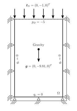
We use here a Terzaghi-type consolidation test enforcing an uniaxial compression on a three-dimensional fluid-saturated poroelastic block placed in an aquarium with non-deformable walls and open top surface which is loaded by gravity and, moreover, instantaneously in $t_{0}=0^{+}$ with an outer normal traction and therefore has incompatible initial data. The schematic test setting of all numerical examples is illustrated with a two-dimensional cut by Fig. 1 (a) and further explained in detail.

We remark that the overall test setting yields a problem which ensures the existence and uniqueness of solutions even with the componentwise taken mixed Dirichlet and Neumann type boundary conditions for the mechanical problem. The contact problem of the mechanical problem, occuring here by hitting the non-deformable walls of the fluid-saturated poroelastic material under load, is resolved here, for simplicity and as usual, by setting physically reasonable homogeneous Dirichlet type boundary data on the displacement field in a componentwise taken sense.

Remark that the test setting yields benchmark problem, since it was already used in [11, 5, 13, 15] in corresponding an one- or two-dimensional way, but we use here fully three-dimensional setting. Remark also that for the generation of the solutions of the displacement and the pressure for the given test problem even the classical one-dimensional test is enough to get satisfying results of physically relevance. Anyhow, we use here the corresponding three-dimensional form since this stresses much more the applied space-time discretisations, the applied fixed-stress iterative solvers as well as the linear solver and preconditioning techniques underneath to show advantages and disadvantages of the approaches, which is in the focus of this work and is of further interest in the current research, and to simplify the verification by comparision with known results of the computed solutions for the reader.

The pressure solution below the constrained top surface includes a Mandel-Cryer effect, which is a pressure overshoot shortly after the initial time since the fluid is not able to escape instantaneously; cf. [13, 14]. This Mandel-Cryer effect is an additional difficulty for non-robust solver strategies as they can appear for iteratively-coupled solvers, e.g. fixed-stress solver technologies for higher-order time discretisations employing a complicated nested Schur complement solver technology, which will be also studied by the following examples. We note that such difficulties can be overcome by using monolithic solver strategies instead of iteratively coupled solvers, but they have the need for an efficient and scalable preconditioning technology which will be studied in our forthcoming work in [1].

All numerical results are computed with the DTM++/biot-fs solver suite which is a frontend solver of the author for the deal.II v8.5.1 library; cf. [2, 8, 5] and [9]. They enforce 10 distributed parallel (MPI) processes each for the parallelisation and distribution of the spatial domain such that each process locally owns 25 mesh cells $K$. Note that different numbers of overall degrees of freedoms need to be computed for different time discretisations of the same piecewise polynomial order in time for the introduced families. In general, discontinuous Galerkin (time) discretisations are more expensive in any terms for the same piecewise polynomial degree as their continuous Galerkin discretisation counterparts.

We optimise all fixed-stress iterative schemes by using $K_{\textnormal{dr}}^{*}=\lambda+2\mu$, with $\lambda$ and $\mu$ being the first and second Lamé parameters as introduced in Sec. 2, as the most optimal $K_{\textnormal{dr}}^{*}$ value under uniaxial loading without deeper knowledge on the problem as it is studied in detail in [3]. We note that the numbers of the fixed-stress iterations is not a measurement of the performance in this work since it has to be shown to lead to non-comparable results due to different tunings. All numerical solvers are tuned in a way that they deliver comparable results in terms of computational efficiency and accuracy.

For the following experiments we let the test setting illustrated by Fig. 1 (a) being the same for all numerical experiments. The spatial domain is set to $\Omega=(0,0.5)\times(0,1)\times(0,0.5)$ with $h=\sqrt{0.03}$ and time interval is $I=(0,0.5)$ with $\tau=\tau_{n}=0.001$. On the top surface, i.e. precisely $\Gamma_{p}=\{(x,1,z)^{T}\in\mathbb{R}^{3}\,|\,(x,z)^{T}\in(0,0.5)^{2}\}$, we prescribe an inhomogeneous pressure boundary condition with $p_{D}=-5$ and a zero flux boundary condition elsewhere for the flow problem. Note that our global pressure solutions and boundary conditions here must be understand as difference to the corresponding reference state. For the mechanical problem we prescribe an uniform compressive traction $\boldsymbol{t}_{N}=(0,-1,0)^{T}$ on the top surface and componentwise mixed homogeneous Dirichlet and homogeneous traction conditions elsewhere. The piecewise polynomial approximation degree in space is choosen such that we have a piecewise triquadratic approximation of the displacement field ($\boldsymbol{Q}_{h}^{2}$ finite element space) and a piecewise trilinear approximation of the pressure ($\text{RT}_{1}$ mixed finite element space). For all material parameters we use the values given in [11, Sec. 5.1].
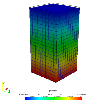
In Fig. 1 (b) the displacement field $\boldsymbol{u}$ is illustrated by warping the domain $\Omega$ and the pressure difference distribution $p$ by the colour at $t=0.1$ for the new dG($1$)-cG($1$) fixed-stress solver for incompatible initial data given by Scheme 1 in Sec. 4.6. For better comparision of the fixed-stress solvers with different time discretisations in the following Sec. 5.1 and 5.2 we compute the mean value of the pressure solution along the embedded one-dimensional line $\boldsymbol{c}_{L}(s)=(s,0.15,0.25)^{T}$ with $s\in(0,0.5)$. Note that the line $\boldsymbol{c}_{L}$ is aligned to a constant pressure layer.

Refer to caption
(a) Schematic test setting.
Refer to caption
(b) Solution for $t=0.1$.
Figure 1: Schematic test setting given by a two-dimensional cut illustration (a) and solution illustration (b) for Sec. 5. In (b) the displacement field $\boldsymbol{u}$ is illustrated by warping the domain $\Omega$ and the pressure difference distribution $p$ by the colour at $t=0.1$ of a three-dimensional Terzaghi-type consolidation test problem with piecewise quadratic displacement and piecewise linear pressure approximation in space and the new dG($1$)-cG($1$) fixed-stress solver for incompatible initial data given by Scheme 1 in Sec. 4.6.

The further structure of this section reads as follows. In Sec. 5.1 we compare the time discretisations dG(0), cG(1) and dG(1), in Sec. 5.2 we study the new dG(1)-cG(1) for incompatible initial data given by Scheme 1 of Sec. 4.6 against the dG(0) and dG(1) time discretisations and in Sec. 5.3 we study the performance of all fixed-stress solvers.

00$0.05$ $0.1$ $0.15$ $0.2$00$1$ $2$ $\displaystyle|\boldsymbol{c}_{L}|^{-1}\int_{\boldsymbol{c}_{L}}p_{\tau,h}^{\ast}(\boldsymbol{x},\cdot)\mathrm{d}\boldsymbol{s}$  over  time $t$ $\textnormal{dG(0)}=:\ast$ $\textnormal{cG(1)}=:\ast$
(a) dG(0) and cG(1).
00$0.05$ $0.1$ $0.15$ $0.2$00$0.5$ $1$ $1.5$ $2$ $\displaystyle|\boldsymbol{c}_{L}|^{-1}\int_{\boldsymbol{c}_{L}}p_{\tau,h}^{\ast}(\boldsymbol{x},\cdot)\mathrm{d}\boldsymbol{s}$  over  time $t$ $\textnormal{dG(0)}=:\ast$ $\textnormal{dG(1)}=:\ast$
(b) dG(0) and dG(1).
Figure 2: Pressure solution on $\boldsymbol{c}_{L}$ for Sec. 5.1.
00$0.05$ $0.1$ $0.15$ $0.2$00$0.5$ $1$ $1.5$ $2$ $\displaystyle|\boldsymbol{c}_{L}|^{-1}\int_{\boldsymbol{c}_{L}}p_{\tau,h}^{\ast}(\boldsymbol{x},\cdot)\mathrm{d}\boldsymbol{s}$  over  time $t$ $\textnormal{dG(0)}=:\ast$ $\textnormal{dG(1)-cG(1)}=:\ast$
(a) dG(0) and dG(1)-cG(1).
00$0.05$ $0.1$ $0.15$ $0.2$00$0.5$ $1$ $1.5$ $2$ $\displaystyle|\boldsymbol{c}_{L}|^{-1}\int_{\boldsymbol{c}_{L}}p_{\tau,h}^{\ast}(\boldsymbol{x},\cdot)\mathrm{d}\boldsymbol{s}$  over  time $t$ $\textnormal{dG(1)}=:\ast$ $\textnormal{dG(1)-cG(1)}=:\ast$
(b) dG(1) and dG(1)-cG(1).
Figure 3: Pressure solution on $\boldsymbol{c}_{L}$ for Sec. 5.2.

5.1 Test case: dG(0), cG(1) and dG(1) for incompatible initial data

In the first numerical study we compare (a) the dG(0) with the cG(1) time discretisations, which are the members of lowest-order type in time in their family, and (b) the dG(0) and the dG(1) time discretisations. The corresponding pressure solutions averaged on $\boldsymbol{c}_{L}$ are illustrated in Fig. 2 (a) and (b).

The dG(0) time discretisation can be re-identified as the classical backward Euler time discretisation, which is known as robust time discretisation, but it delivers only piecewise constant approximation in time. The numerical solution of the dG(0) fixed-stress solver match with the known data from the literature; cf. [11, 5].

In contrast, the cG(1) fixed-stress solver produces an unphysically oscillating and therefore unsuitable numerical solution. Note that even a monolithic solver for the presented cG(1) time discretisation has the same issue with unphysical oscillations in the case of incompatible data. This result of the cG(1) solver is unsatisfying since it has a piecewise linear approximation in time for comparable computational costs as the dG(0) solver which will be analysed in Sec. 5.3.

Secondly, in Fig. 2 (b) we compare the dG(0) and dG(1) fixed-stress solver solutions. For $t\in(0,0.045)$ the pressure results are only slightly different, but after the Mandel-Cryer effect the dG(1) fixed-stress solver gets into trouble, which results in unforeseeable number of fixed-stress iterations. As we use here the dG(1) fixed-stress solver without specific tuning to the test problem to allow for comparable results for Sec. 5.3, the pressure solution clearly shows imprecise results for $t>0.045$. Note that this issue can be resolved by enforcing higher tolerance values within the complex and nested linear system solver but then the simulation wall time will increase massively. Remark that we have presented the needed complex inner solver structure for the dG(1) fixed-stress solver in [5, 4].

5.2 Test case: dG(1)-cG(1) against dG(0) and dG(1) for incompatible initial data

In the second numerical study we compare (a) the dG(0) time discretisation with the new dG(1)-cG(1) coupled time discretisation given by Scheme 1 in Sec. 4.6 and (b) the dG(1) time discretisation with the new dG(1)-cG(1) time discretisation. The corresponding pressure solutions averaged on $\boldsymbol{c}_{L}$ are illustrated in Fig. 3 (a) and (b).

In contrast to Sec. 5.1, the new dG(1)-cG(1) fixed-stress solver computes suitable numerical solution which matches mostly with the dG(0) solution as it is illustrated in Fig. 3 (a). Note that the slight difference in the solutions are expected from different convergence orders of the time discretisations coming from the piecewise constant and, respectively, piecewise linear approximations in time. This hypothesis has to be shown with rigorous error analysis in a future work. Additionally remark that the spatial discretisation used for all test problems was initially converged such that only differences for the time discretisation can be clearly presented here.

In Fig. 3 (b) we study the piecewise linear approximations in time with the global dG(1) fixed-stress solver and the new dG(1)-cG(1) fixed-stress solver. The pressure solutions of the new dG(1)-cG(1) solver fit to the solutions of the dG(1) fixed-stress solver for $t<0.045$. The new approach does not match with non-tuned dG(1) fixed-stress solver for $t>0.045$, which let us lead to interpret the overall dG(1) numerical solution as unsatisfying result for the test problem and solver tolerances here. Remark that we have studied in [5] that also the dG(1) fixed-stress solver gives satisfying numerical approximations.

5.3 Performance comparision: dG(0), dG(1)-cG(1), cG(1) and dG(1)

In this subsection we analyse the computational performance and efficiency of the fixed-stress solvers dG(0), cG(1), dG(1) and the new dG(1)-cG(1) used in Sec. 5.1 and 5.2 by giving the simulation wall times. Note that not the simulation wall time (sometimes denoted as CPU time) itself is a measurement of the efficiency, instead the difference between the wall times of the solvers demonstrate the efficiency. We remark again that our implementation in the DTM++/biot-fs solver suite leads to comparable solvers since most of the code is reused in a hierarchical and modularised way; cf. [2].

The simulation wall times for the fixed-stress solvers dG(0), cG(1), dG(1) and the new dG(1)-cG(1) fixed-stress solvers differ in a major way:

  • $\bullet$

    dG(0) fixed-stress solver: 56 seconds,

  • $\bullet$

    dG(1)-cG(1) fixed-stress solver: 90 seconds,

  • $\bullet$

    cG(1) fixed-stress solver: 184 seconds and

  • $\bullet$

    dG(1) fixed-stress solver: 1573 second.

to fully compute the problem given in Sec. 5 for $I=(0,0.5)$ with $\tau=\tau_{n}=0.001$ for all solvers and including all preprocessing and postprocessing steps such as parsing the input parameters, grid generation, assembly as well as data output of the global solution. Note that the real cpu time, not the simulation wall time, can be computed by multiplying the respective wall time by the factor of 10 since we have used 10 MPI processes for each simulation. Again, as it is studied in detail in Sec. 5.1 and 5.2, the solution of the cG(1) fixed-stress solver is not feasible to be used while the solution of the new dG(1)-cG(1) approach given by Scheme 1 in Sec. 4.6 yields accurate numerical solutions. Moreover, the new approach performs the complete simulation with mostly the same simulation wall time as the dG(0) fixed-stress solver. We remark that the gap between the wall times comes from solving with the dG(1) fixed-stress solver on $I_{1}$ in the new approach.

We finally remark that the obvious lack of accuracy, performance and efficiency of the dG(1)-fs solver comes here due to the fixed-stress iterative approach, in a forthcoming work we show that this can be resolved by a monolithic solver approach using an efficient and flexible preconditioning technology; [1].

6 Conclusions

In this work we studied in detail Biot’s quasi-static system of poroelasticity which we have established from conservation and balance laws and other physical principles under necessary and natural assumptions on the data. Then we presented the fixed-stress iterative approach for decoupling the flow and the mechanical subproblems for the infinite-dimensional space-time problem. Further we studied the application of discontinuous and continuous Galerkin time discretisations of arbitrary polynomial order in time. We presented details for the assemblies of the mixed discretisation in space in a way such that they can be reused for an arbitrary time discretisation and for splitting or monolithic schemes. A new dG($r$)-cG($r$) in time approach, using dG($r$) and cG($r$) time discretisations in different time regions, was introduced. With a three-dimensional numerical experiment of physical relevance we studied the stability and computational efficiency of the presented schemes. The new dG($1$)-cG($1$) approach has been shown numerically to be as robust and computationally efficient as the classically used backward Euler time discretisation while the global (higher-order) dG($1$) in time fixed-stress approach did not yield satisfying results. The application of monolithic solvers instead of iteration schemes will be done in a forthcoming work; [1]. The stability and convergence of the new dG($1$)-cG($1$) in time approach needs to be rigorously analysed in a future work.

References

  • [1] U. Köcher, High-order space-time-parallel monolithic solvers and preconditioning for the Biot poroelasticity system, in preparation, 2018.
  • [2] U. Köcher, The DTM++/biot-fs suite: Efficient high-order fixed-stress solvers for Biot’s system, in preparation, https://bitbucket.org/dtmproject, p.1-6, 2018.
  • [3] J.W. Both and U. Köcher, Numerical investigation on the fixed-stress splitting scheme for Biot’s equations: Optimality of the tuning parameter, Numer. Math. Adv. Appl. ENUMATH 2017, accepted, arXiv:1801.08352, 2017.
  • [4] M. Bause and F.A. Radu and U. Köcher, Space-time finite element approximation of the Biot poroelasticity system with iterative coupling, Comput. Meth. Appl. Mech. Engrg. 320:745-768, 10.1016/j.cma.2017.03.017, 2017.
  • [5] M. Bause and U. Köcher, Iterative coupling of variational space-time methods for Biot’s system of poroelasticity, Numer. Math. Adv. Appl. ENUMATH 2015:143-151, 10.1007/978-3-319-39929-4_15, 2016.
  • [6] M. Bause and F.A. Radu and U. Köcher, Error analysis for discretizations of parabolic problems using continuous finite elements in time and mixed finite elements in space, Numer. Math. 137(4):773-818, 10.1007/s00211-017-0894-6, 2017.
  • [7] M. Bause and U. Köcher, Variational time discretization for mixed finite element approximations of nonstationary diffusion problems, J. Comput. Appl. Math. 289:208-224, 10.1016/j.cam.2015.02.015, 2015.
  • [8] U. Köcher, Variational space-time methods for the elastic wave equation and the diffusion equation, Ph.D. thesis, Department of Mechanical Engineering of the Helmut-Schmidt-University, University of the German Federal Armed Forces Hamburg, p. 1-188, urn:nbn:de:gbv:705-opus-31129, 2015.
  • [9] D. Arndt and W. Bangerth and D. Davydov and T. Heister and L. Heltai and M. Kronbichler and M. Maier and J.-P. Pelteret and B. Turcksin and D. Wells, The deal.II library, version 8.5, J. Numer. Math. 25(3):137-146, 10.1515/jnma-2017-0058, 2017.
  • [10] J.A. White and R.I. Borja, Stabilized low-order finite element methods for coupled solid-deformation/fluid-diffusion and their application to fault zone transients, Comput. Meth. Appl. Mech. Engrg. 197(49-50):4353-4366, 10.1016/j.cma.2008.05.015, 2008.
  • [11] B. Jha and R. Juanes, A locally conservative finite element framework for the simulation of coupled flow and reservoir geomechanics, Acta Geotech. 2(3):139-153, 10.1007/s11440-007-0033-0, 2007.
  • [12] P.J. Phillips and M.F. Wheeler, A coupling of mixed and continuous Galerkin finite element methods for poroelasticity I, II, Comput. Geosci. 11:131-158, 10.1007/s10596-007-9045-y, 2007.
  • [13] C.W. Cryer, A comparision of the three-dimensional consolidation theories of Biot and Terzaghi, Q. J. Mech. Appl. Math. 16(4):401-412, 10.1093/qjmam/16.4.401, 1963.
  • [14] J. Mandel, Consolidation des sols (étude mathématique), Géotechnique 3(7):287-299, 10.1680/geot.1953.3.7.287, 1953.
  • [15] K. Terzaghi, Theoretical soil mechanics, Wiley, New York, 10.1002/9780470172766, 1943.
  • [16] R. Showalter, Diffusion in poro-elastic media, J. Math. Anal. Appl. 251(1):310-340, 10.1006/jmaa.2000.7048, 2000.
  • [17] R. Showalter and U. Stefanelli, Diffusion in poro‐plastic media, Math. Methods Appl. Sci. 27(18):2131-2151, 10.1002/mma.541, 2004.
  • [18] A. Mikelić and M.F. Wheeler, Theory of the dynamic Biot-Allard equations and their link to the quasi-static Biot system, J. Math. Phys. 53(123702):1-16, 10.1063/1.4764887, 2012.
  • [19] J.W. Both and M. Borregales and J.M. Nordbotten and K. Kumar and F.A. Radu, Robust fixed stress splitting for Biot’s equations in heterogeneous media, Appl. Math. Lett. 68:101-108, 10.1016/j.aml.2016.12.019, 2017.
  • [20] B. Wang, Parallel simulation of coupled flow and geomechanics in porous media, PhD. thesis, University of Texas at Austin, 2014.
  • [21] A. Mikelić and B. Wang and M.F. Wheeler, Numerical convergence of iterative coupling for coupled flow and geomechanics, Comput. Geosci. 18(3-4):325-341, 10.1007/s10596-013-9393-8, 2014.
  • [22] A. Mikelić and M.F. Wheeler, Convergence of iterative coupling for coupled flow and geomechanics, Comput. Geosci. 17(3):455-461, 10.1007/s10596-012-9318-y, 2013.
  • [23] J. Kim and H.A. Tchelepi and R. Juanes, Stability and convergence of sequential methods for coupled flow and geomechanics: Drained and undrained splits, Comput. Meth. Appl. Mech. Engrg. 200(23-24):2094-2116, 10.1016/j.cma.2011.02.011, 2011.
  • [24] J. Kim and H.A. Tchelepi and R. Juanes, Stability and convergence of sequential methods for coupled flow and geomechanics: Fixed-stress and fixed-strain splits, Comput. Meth. Appl. Mech. Engrg. 200(13-16):1951-1606, 10.1016/j.cma.2010.12.022, 2011.
  • [25] A. Settari and F.M. Mourits, A coupled reservoir and geomechanical simulation system, Soc. Pet. Engrg. J. 3(3):219-226, 10.2118/50939-PA, 1998.
  • [26] M.A. Biot, General theory of three-dimensional consolidation, J. Appl. Phys. 12(2):155-164, 10.1063/1.1712886, 1941.
  • [27] M.A. Biot, Acoustics, elasticity, and thermodynamics of porous media: Twenty-one papers, Ed. I. Tolstoy, Acoustical Society of America, New York, 1992.
  • [28] J.T. Fredrich and J.G. Arguello and G.L. Deitrick and E.P. De Rouffignac, Geomechanical modeling of reservoir compaction, surface subsidence, and casing damage at Belridge diatomite field, SPE Reserv. Eval. Eng. 3(4):348-359, 10.2118/65354-PA, 2000.
  • [29] E. Detournay and A.H.-D. Cheng, Fundamentals of poroelasticity, Ch. 5 in Comprehensive Rock Engineering: Principles, Practice and Projects, Vol. II, Analysis and Design Method, Pergamon, pp. 113-171, 1993.
  • [30] O. Coussy, Mechanics of porous media, John Wiley & Sons, Chichester, England, 1995.
  • [31] G. Allaire, Homogenization of the Stokes flow in a connected porous medium, Asymptotic Anal. 2:203-222, 1989.
  • [32] J.H. Argyris and D.W. Scharpf, Finite elements in time and space, Aer. J. Royal Aer. Soc. 73:1041-1044, 1969.
  • [33] C. Dawson and J. Proft, Discontinuous and coupled continuous/discontinuous Galerkin methods for the shallow water equations, Comput. Meth. Appl. Mech. Engrg. 191(41-42):4721-4746, 10.1016/S0045-7825(02)00402-4, 2002.