Modelling thermo-electro-mechanical effects
in orthotropic cardiac tissue

Abstract

In this paper we introduce a new mathematical model for the active contraction of cardiac muscle, featuring different thermo-electric and nonlinear conductivity properties. The passive hyperelastic response of the tissue is described by an orthotropic exponential model, whereas the ionic activity dictates active contraction incorporated through the concept of orthotropic active strain. We use a fully incompressible formulation, and the generated strain modifies directly the conductivity mechanisms in the medium through the pull-back transformation. We also investigate the influence of thermo-electric effects in the onset of multiphysics emergent spatiotemporal dynamics, using nonlinear diffusion. It turns out that these ingredients have a key role in reproducing pathological chaotic dynamics such as ventricular fibrillation during inflammatory events, for instance. The specific structure of the governing equations suggests to cast the problem in mixed-primal form and we write it in terms of Kirchhoff stress, displacements, solid pressure, electric potential, activation generation, and ionic variables. We also propose a new mixed-primal finite element method for its numerical approximation, and we use it to explore the properties of the model and to assess the importance of coupling terms, by means of a few computational experiments in 3D.

92C10, 74S05, 65M60, 74F25.

1 Introduction

Temperature variations may have a direct impact on many of the fundamental mechanisms in the cardiac function (Wilson and Crandall, 2011). Substantial differences have been reported in the conduction velocity and spiral drift of chaotic electric potential propagation in a number of modelling and computationally-oriented studies (Filippi et al., 2014), and several experimental tests confirm that this is the case not only for cardiac tissue, but for other excitable systems (Gizzi et al., 2010; Kienast et al., 2017). The phenomenon is however not restricted to electrochemical interactions, but it also might affect mechanical properties (Hill and Sec, 1938; Lawton, 1954; Sugi and Pollack, 1998). Indeed, cardiac muscle is quite sensitive to mechanical stimulation and deformation patterns can be very susceptive to external agents such as temperature. For instance, enhanced tissue heterogeneities can be observed when the medium is exposed to altered thermal states, and in turn these can give rise to irregular mechano-chemical dynamics. A few examples that relate to experimental observations from epicardial and endocardial activity on canine right ventricles at different temperatures, as well as tachycardia and other fibrillation mechanisms occurring due to thermal unbalance, can be found in e.g. Filippi et al. (2014). These scenarios can be related to extreme conditions encountered during heat strokes and sports-induced fatigue (easily reaching 41^∘C), and localisation of other thermal sources such as ablation devices; but also to surgery or therapeutical procedures (in open-chest surgery tissues might be exposed to cold air in the operating theatre at 25^∘C), or due to extended periods of exposure to even lower temperatures that can occur during shipwrecks or avalanches. It is not striking that temperature effects might affect the behaviour of normal electromechanical heart activity. However the precise form that these mechanisms manifest themselves is not at all obvious. This is, in part, a consequence of the nonlinear character of the thermo-electro-mechanical coupling. For instance, one can show that localised thermal gradients might destabilise the expected propagation of the electric wave, as well as change the mechanical behaviour of anisotropic contraction. Our goal is to investigate the role of the aforementioned effects in the development and sustainability of cardiac arrhythmias. These complex emerging phenomena originate from multifactorial and multiphysical interactions (Qu et al., 2014), and they are responsible for a large number of cases of pathological dysfunction and casualties. The model we propose here has potential therefore in the investigation of mechanisms provoking such complex dynamics, in particular those arising during atrial and ventricular fibrillation.

Even if computational models for the electromechanics of the heart are increasingly complex and account for many multiphysics and multiscale effects (see e.g. Colli Franzone et al., 2016; Trayanova and Rice, 2011; Quarteroni et al., 2017), we are only aware of one recent study (Collet et al., 2017) that addresses similar questions to the ones analysed here. However that study is restricted to one-dimensional domains, it uses the two-variable model from Nash and Hunter (2000), and it assumes an active stress approach for a simplified neo-Hookean material in the absence of an explicit stretch state. Our phenomenological framework also uses a temperature-based two-variable model, but in contrast, it additionally includes a nonlinear conductivity representing a generalised diffusion mechanism intrinsic to porous-medium electrophysiology (Hurtado et al., 2016). We postulate then an extended model that also accounts for active deformation of the tissue, where the specific form of the electromechanical coupling is dictated by an adaptation of the orthotropic active strain framework proposed in Rossi et al. (2014).

We have structured the contents of this paper in the following manner. Section 2 discusses a combination of phenomenological and physiological coupled models from thermo-electric and thermo-mechanic dynamics being local (potentially sub-cellular in a physiological model), tissue, and organ-scale levels. We introduce in Section 3 a new mixed-primal finite element scheme for the solution of the set of governing equations (in particular using the Kirchhoff stress as additional unknown), where we provide also some details about its computational realisation. All of our numerical tests are collected in Section 4, including conduction velocity assessment, and a few simulations regarding normal and arrhythmic dynamics in simplified 3D domains. We then conclude in Section 5 with a summary and a discussion on the limitations and envisaged extensions of this study.

2 A new model for thermo-electric active strain

In this section we provide an abridged derivation of the set of partial differential equations describing the multiscale coupling between electric, thermal, mechanical, and ionic processes; which are, in principle, valid for general excitable and deformable media.

2.1 Muscle contraction via the active strain approach

Let $\Omega\subset{{\mathbb{R}}^{3}}$ denote a deformable body with piecewise smooth boundary $\partial\Omega$, regarded in its reference configuration, and denoted by ${\boldsymbol{\nu}}$, the outward unit normal vector on $\partial\Omega$. The kinematical description of finite deformations regarded on a time interval $t\in(0,t_{\text{final}}]$ is made precise as follows. A material point in $\Omega$ is denoted by ${\boldsymbol{x}}$, whereas ${{\boldsymbol{x}}_{t}-{\boldsymbol{x}}=}{\boldsymbol{u}}(t):\Omega\to{{\mathbb{R}}^{3}}$ will denote the displacement field characterising its new position ${\boldsymbol{x}}_{t}$ within the body $\Omega_{t}$ in the current, deformed configuration. The tensor ${\mathbf{F}}:={\mathbf{I}}+\nabla{\boldsymbol{u}}$ is the gradient (applied with respect to the fixed material coordinates) of the deformation map; its Jacobian determinant, denoted by $J=\det{\mathbf{F}}$, measures the solid volume change during the deformation; and ${\mathbf{C}}={\mathbf{F}}^{\tt t}{\mathbf{F}}$ is the right Cauchy-Green deformation tensor on which all strain measures will be based (here the superscript $()^{\tt t}$ denotes the transpose operator). The first isotropic invariant controlling deviatoric effects is $I_{1}({\mathbf{C}})={\rm tr}\,{\mathbf{C}}$, and for generic unitary vectors ${\boldsymbol{f}_{0}},{\boldsymbol{s}_{0}}$, the scalars $I_{4,f}({\mathbf{C}})={\boldsymbol{f}_{0}}\cdot({\mathbf{C}}{\boldsymbol{f}_{0}})$, $I_{8,fs}({\mathbf{C}})={\boldsymbol{f}_{0}}\cdot({\mathbf{C}}{\boldsymbol{s}_{0}})$ are direction-dependent pseudo-invariants of ${\mathbf{C}}$ measuring fibre-aligned stretch (see e.g. Spencer, 1989). As usual, ${\mathbf{I}}$ denotes the 3$\times$3 identity matrix. In the remainder of the presentation we will restrict all space differential operators to the material coordinates.

Next we recall the active strain model for ventricular electromechanics as introduced in Nobile et al. (2012). There, the contraction of the tissue results from activation mechanisms governed by internal variables and incorporated into the finite elasticity context using a virtual multiplicative decomposition of the deformation gradient into a passive (purely elastic) and an active part ${\mathbf{F}}={\mathbf{F}}_{\!E}{\mathbf{F}}_{\!A}$, defined in general, triaxial form

$${{\mathbf{F}}_{\!A}={\mathbf{I}}+\gamma_{f}{\boldsymbol{f}_{0}}({\boldsymbol{x}})\otimes{\boldsymbol{f}_{0}}({\boldsymbol{x}})+\gamma_{s}{\boldsymbol{s}_{0}}({\boldsymbol{x}})\otimes{\boldsymbol{s}_{0}}({\boldsymbol{x}})+\gamma_{n}{\boldsymbol{n}_{0}}({\boldsymbol{x}})\otimes{\boldsymbol{n}_{0}}({\boldsymbol{x}}).}$$ (2.1)

The coefficients $\gamma_{i}$, with $i=f,s,n$, are smooth scalar functions encoding the macroscopic stretch in specific directions, whose precise definition will be postponed to Section 2.3. The inelastic contribution to the deformation modifies the size of the cardiac fibres, and then compatibility of the motion is restored through an elastic deformation accommodating the active strain distortion. The triplet $({\boldsymbol{f}_{0}}({\boldsymbol{x}}),{\boldsymbol{s}_{0}}({\boldsymbol{x}}),{\boldsymbol{n}_{0}}({\boldsymbol{x}}))$ represents a coordinate system pointing in the local direction of cardiac fibres, transversal sheetlet compound, and normal cross-fibre direction ${\boldsymbol{n}_{0}}({\boldsymbol{x}})={\boldsymbol{f}_{0}}({\boldsymbol{x}})\times{\boldsymbol{s}_{0}}({\boldsymbol{x}})$.

Constitutive relations defining the material properties and underlying microstructure of the myocardial tissue will follow the orthotropic model proposed in Holzapfel and Ogden (2009), for which the strain energy function and the first Piola-Kirchhoff stress tensor (after applying the active strain decomposition) read respectively

$$\Psi({\mathbf{F}}_{E})=\frac{a}{2b}e^{b(I^{E}_{1}-{3})}+\dfrac{a_{fs}}{2b_{fs}}\bigl{[}e^{b_{fs}(I_{8,fs}^{E})^{2}}-1\bigr{]}+\sum_{i\in\{f,s\}}\dfrac{a_{i}}{2b_{i}}\bigl{[}e^{b_{i}{((I^{E}_{4,i}-1)_{+})^{2}}}-1\bigr{]},\quad{\mathbf{P}}=\frac{\partial\Psi}{\partial{\mathbf{F}}}-pJ{\mathbf{F}}^{-{\tt t}},$$ (2.2)

where $a,b,a_{i},b_{i}$ with $i\in\{f,s,fs\}$ are material parameters, $p$ denotes the solid hydrostatic pressure, and have used the notation $(x)_{+}:=\max\{x,0\}$. Switching off the anisotropic contributions acting on ${\boldsymbol{s}_{0}}$ and ${\boldsymbol{n}_{0}}$ (but not the shear term) under compression ensures that the associated terms in the strain energy function (in both the pure passive and active-strain formulations) are strongly elliptic (Pezzuto et al., 2014) (these will be the terms appearing on the second diagonal block of the weak formulation from Section 3, the block corresponding to displacements), however the overall problem will remain of a saddle-point structure.

The modified elastic invariants $I_{i}^{E}$ are functions of the coefficients $\gamma_{i}$ and the invariant and pseudo invariants as follows

$$I_{1}^{E} ={\biggl{[}1-\frac{\gamma_{n}(\gamma_{n}+2)}{(\gamma_{n}+1)^{2}}\biggr{]}I_{1}+\biggl{[}\frac{\gamma_{n}(\gamma_{n}+2)}{(\gamma_{n}+1)^{2}}-\frac{\gamma_{f}(\gamma_{f}+2)}{(\gamma_{f}+1)^{2}}\biggr{]}I_{4,f}+\left[\frac{\gamma_{n}(\gamma_{n}+2)}{(\gamma_{n}+1)^{2}}-\frac{\gamma_{s}(\gamma_{s}+2)}{(\gamma_{s}+1)^{2}}\right]I_{4,s}},$$

$$I_{4,f}^{E} =\dfrac{I_{4,f}}{\left(\gamma_{f}+1\right)^{2}},\quad I_{4,s}^{E}=\dfrac{I_{4,s}}{\left(\gamma_{s}+1\right)^{2}},\quad I_{8,fs}^{E}=\dfrac{I_{8,fs}}{\left(\gamma_{f}+1\right)\left(\gamma_{s}+1\right)}.$$

Accordingly, the active strain and consequently the force associated to the active part of the total stress, will receive contributions acting distinctively on each direction ${\boldsymbol{f}_{0}}({\boldsymbol{x}}),{\boldsymbol{s}_{0}}({\boldsymbol{x}}),{\boldsymbol{n}_{0}}({\boldsymbol{x}})$.

The balance of linear momentum together with the incompressibility constraint are written, when posed in the inertial reference frame and under pseudo-static mechanical equilibrium, in the following way

$$-\boldsymbol{\nabla}\cdot{\mathbf{P}} =\rho_{0}{\boldsymbol{b}} \text{in }\Omega\times(0,t_{\mathrm{final}}],$$ (2.3a)

$$\rho J-\rho_{0} =0 \text{in }\Omega\times(0,t_{\mathrm{final}}],$$ (2.3b)

where $\rho_{0},\rho$ are the reference and current medium density, and ${\boldsymbol{b}}$ is a vector of body loads. Furthermore, the balance of angular momentum translates into the condition of symmetry of the Kirchhoff stress tensor ${\mathbf{\Pi}}={\mathbf{P}}{\mathbf{F}}^{\tt t}$, which is in turn encoded into the momentum and constitutive relations (2.3a), (2.2), and (2.1).

Following the notation in Chavan et al. (2007), the contribution to stress that does not include pressure explicitly is denoted as $\mathcal{G}({\boldsymbol{u}}):=\frac{\partial\Psi}{\partial{\mathbf{F}}}{\mathbf{F}}^{\tt t}$, and therefore we have the constitutive relation

$${\mathbf{\Pi}}=\mathcal{G}({\boldsymbol{u}})-pJ{\mathbf{I}}.$$ (2.4)

2.2 A modified Karma model for cardiac action potential

Let us denote by $I_{\rm ext}$ a spatio-temporal external electrical stimulus applied to the medium. On the undeformed configuration we proceed to write the following monodomain equations describing the transmembrane potential propagation and the dynamics of slow recovery currents according to a specific temperature $T$:

$$\frac{\partial v}{\partial t}-\nabla\cdot{\left[{\mathbf{D}}(v,{\mathbf{F}})\,\nabla v\right]} =\dfrac{f(v,n)}{\tau_{v}(T)}+I_{\rm ext} \text{in }\Omega\times(0,t_{\mathrm{final}}],$$ (2.5a)

$$\frac{dn}{dt} =\dfrac{g(v,n)}{\tau_{n}(T)} \text{in }\Omega\times(0,t_{\mathrm{final}}],$$ (2.5b)

where the unknowns are the transmembrane potential, $v$, and the recovery variable, $n$. This reaction-diffusion system is endowed with the following specifications, taking the membrane model proposed in Karma (1994), and adapting it to include thermo-electric effects following the development in Gizzi et al. (2017b)

$$f(v,n) :=-v+[v^{*}-\mathcal{S}(n)][1-\tanh(v-v_{\star})]\frac{v^{2}}{2},$$ (2.6a)

$$g(v,n) :=\mathcal{R}(n)\mathcal{H}(v-v_{n})-[1-\mathcal{H}(v-v_{n})]n,$$ (2.6b)

$$\mathcal{R}(n) :=\dfrac{1-(1-e^{-L})n}{1-e^{-L}},\qquad\quad\mathcal{S}(n):=n^{M},$$ (2.6c)

$$\tau_{v}(T) :=\dfrac{\tau_{v}^{0}}{1+\beta(T-T_{0})},\quad\tau_{n}(T):=\tau_{n}^{0}\,{Q_{10}(T)}.$$ (2.6d)

As in the original phenomenological model from Karma (1994), here $\mathcal{H}(x)$ stands for the Heaviside step function, i.e. $\mathcal{H}(x)=0$ for $x\leq 0$ and $\mathcal{H}(x)=1$ for $x>0$. The (unit-less) transmembrane potential assumes values in $[-1,5]$, and the resting state of the dynamical system is $(v,n)=(0,0)$. The function $\mathcal{R}(n)$ acts as a nonlinear modulator of the time-frame between the end of an action potential pulse and the beginning of the next one (diastolic interval), as well as the duration of the subsequent action potential pulse. The dispersion map $\mathcal{S}(n)$ is based on experimental restitution properties and it relates the instantaneous speed of the action potential front-end at a given spatial point, with the time elapsed since the back-end of a previous pulse that has passed through the same location. In turn, these functions are tuned by the parameters $L,M$, respectively. With the specification (2.6d) we are extending the existing models by including an Arrhenius exponential law that modifies the dynamics of the gating variable through the function $Q_{10}=\mu^{-(T-T_{0})/10}$. This term characterises the action of temperature through the mechanism of ionic feedback. In this expression, $T_{0}$ represents the reference temperature, i.e. $37^{\circ}{\rm C}$, and the law remains valid within a 10-degrees range. Furthermore, the so-called Moore term defining the time constant $\tau_{v}(T)$ associated to the transmembrane voltage is assumed to follow a linear variation with $T$.

The model from Karma (1994) has been designed specifically for cardiac tissue and it has been used in many high-resolution 2D and 3D electrophysiological studies that match various types of experimental data (Gizzi et al., 2017b). A number of more accurate physiological cellular models are available from the literature, but we restrict to (2.6) as the complexity in our model resides more in the multi-field coupling framework and in its suitability for large scale electromechanical simulations. Extensions to the two-variable model in (2.5) that stay on the phenomenological realm include the three and four-variable systems proposed in Fenton and Karma (1998); Bueno-Orovio et al. (2008), and they provide further experimental validation of the suitability of simplified models for the study of a wide class of physiological and pathological scenarios. More specific aspects of possible model extensions will be discussed in Section 5. An additional generalisation with respect to Karma (1994) is the self-diffusion due to voltage and the account for anisotropy in the diffusion. Due to the Piola transformation (forcing a compliance of the diffusion tensor using the deformation gradients), the conductivity tensor ${\mathbf{D}}(\cdot,\cdot)$ in (2.5a) depends nonlinearly on the deformation gradient ${\mathbf{F}}$, whereas self-diffusion is here taken as the potential-dependent diffusivity proposed in Gizzi et al. (2017b), but appropriately modified to incorporate information about preferred directions of diffusivity according to the microstructure of the tissue. This model is motivated by diffusion in porous media (Vazquez, 2006), which has been applied to cardiac tissue in Hurtado et al. (2016), justified by the porous nature of the medium (Lee et al., 2009) and by the multiscale character of diffusion (intercalated discs and gap junctions at the cell level and micro-tubuli at the subcelullar scale, Weinberg et al., 2017). More precisely, we set

$${\mathbf{D}}(v,{\mathbf{F}})=[D_{0}/2+D_{1}v+D_{2}v^{2}]J{\mathbf{C}}^{-1}+D_{0}/2J{\mathbf{F}}^{-1}{\boldsymbol{f}\otimes\boldsymbol{f}}{\mathbf{F}}^{-T},$$ (2.7)

where $\boldsymbol{f}={\mathbf{F}}{\boldsymbol{f}_{0}}$, and where the values taken by the parameters $D_{i}$, $i=0,1,2$ (as well as all remaining model constants) are displayed in Table 3.1, below. Note that here the diffusivity is mainly affected by the fibre-to-fibre connections, and the presence of $J{\mathbf{C}}^{-1}$ suggests a strain-enhanced tissue conductivity, also referred to as geometric feedback (Colli Franzone et al., 2016). The constants $D_{1},D_{2}$ encode the effect of linear and quadratic self-diffusion, and they have special importance at the depolarisation plateau phase, since they modify the speed and action potential duration of the propagating waves. We also note that even for resting transmembrane potential, the conductivity tensor remains positive definite.

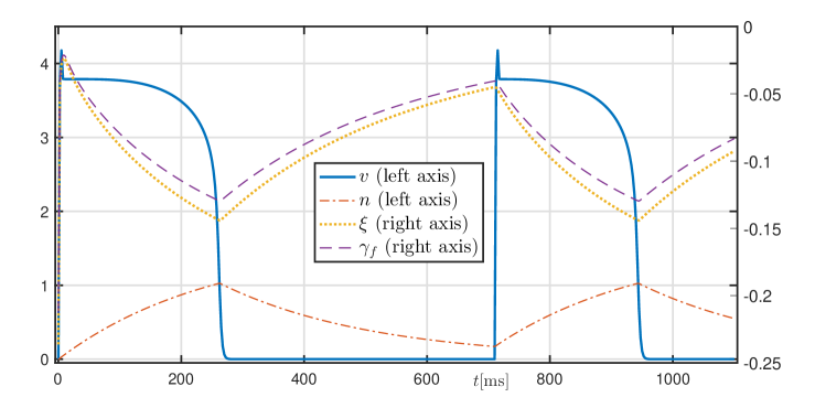
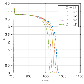
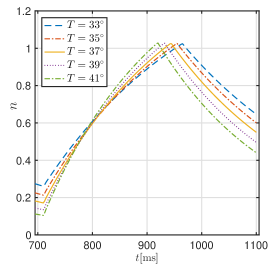
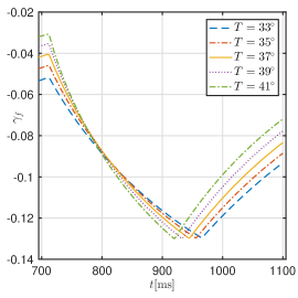
Figure 2.1: Top: kinetics of voltage, gating variable (left axis) and cell shortening with active strain function (right axis) plotted against time. Bottom: Variations of the dynamics of the coupled thermoelectric model according to temperature. The variations of the active strain and myocyte shortening coincide and therefore the latter are not shown.

2.3 Activation mechanisms

A constitutive equation for the activation functions $\gamma_{i}$ in terms of the microscopic cell shortening $\xi$ is adapted from Rossi et al. (2014) as follows

$$\gamma_{f}(\xi)={\gamma_{0}}\xi,\quad\gamma_{s}(\xi)=(1+{\gamma_{0}}\xi)^{-1}(1+K_{0}{\gamma_{0}}\xi)^{-1}-1,\quad\gamma_{n}(\xi)=K_{0}{\gamma_{0}}\xi,$$ (2.8)

where $\gamma_{0}$ is a positive constant that can control the intensity of the activation, and where the specific relation between the myocyte shortening $\xi$ and the dynamics of slow ionic quantities (in the context of our phenomenological model, only $n$) is made precise using the following law

$$\frac{d\xi}{dt}=\dfrac{\ell(\xi,n)}{\tau_{\xi}(T)}\qquad\text{in }\Omega\times(0,t_{\mathrm{final}}],$$ (2.9)

where, in analogy to (2.6), the dynamics of the myocyte shortening are here additionally modulated by a temperature-dependent constant

$$\ell(\xi,n):=K_{1}{\xi^{2}}(1+n)^{-1}-K_{2}{n},\qquad\tau_{\xi}(T):=\tau_{\xi}^{0}\,{\tilde{Q}_{10}(T)}.$$ (2.10)

Here $\tilde{Q}_{10}(T)=\tilde{\mu}^{-(T-T_{0})/10}$. The dynamics of these quantities can be observed in the top panel of Figure 2.1, for the case of base temperature and applying two pacing cycles. Examples of the dynamics of the thermo-electric quantities on the second cycle, and for varying temperatures are collected in the bottom plots of Figure 2.1. The structure of (2.9) suggests that thermo-electric effects could be similarly incorporated in other models for cellular activation (depending on cross-bridge transitions (Land et al., 2017), on calcium - stretch rate couplings in a viscoelastic setting (Eisner et al., 2017), or using phenomenological descriptions), that is through a phenomenological rescaling with $\tau_{\xi}$. However, a deeper understanding on the precise modification of ionic activity in the presence of temperature gradients would be a much more difficult task.

2.4 Initial and boundary conditions

Equations (2.3a)-(2.3b) will be supplemented either with mixed normal displacement-traction boundary conditions

$${\boldsymbol{u}}\cdot{\boldsymbol{\nu}}=0\quad\text{on}\quad\partial\Omega_{D}\times(0,t_{\mathrm{final}}],\qquad\text{and}\qquad{\mathbf{P}}{\boldsymbol{\nu}}=p_{N}J{\mathbf{F}}^{-\tt t}{\boldsymbol{\nu}}\quad\text{on}\quad\partial\Omega_{N}\times(0,t_{\mathrm{final}}],$$ (2.11)

(where $\partial\Omega_{D}$,$\partial\Omega_{N}$ conform a disjoint partition of the boundary, the traction written in terms of the first Piola-Kirchhoff stress tensor is ${\boldsymbol{t}}={\mathbf{P}}{\boldsymbol{\nu}}$, and the term $p_{N}$ denotes a possibly time-dependent prescribed boundary pressure), or alternatively with Robin conditions on the whole boundary

$${\mathbf{P}}{\boldsymbol{\nu}}+\eta J{\mathbf{F}}^{-\tt t}{\boldsymbol{u}}=\boldsymbol{0}\qquad\text{on}\quad\partial\Omega\times(0,t_{\mathrm{final}}],$$ (2.12)

which account for stiff springs connecting the cardiac medium with the surrounding soft tissue and organs (whose stiffness is encoded in the scalar $\eta$). On the other hand, for the nonlinear diffusion equation (2.5a) we prescribe zero-flux boundary conditions representing insulated tissue

$${\mathbf{D}}(v,{\mathbf{F}})\,\nabla v\cdot{\boldsymbol{\nu}}=0\qquad\text{on }\partial\Omega\times(0,t_{\mathrm{final}}].$$ (2.13)

Finally, the coupled set of equations is closed after defining adequate initial data for the transmembrane potential and for the internal variables $\xi,n$:

$$v({\boldsymbol{x}},0)=v_{0}({\boldsymbol{x}}),\quad n({\boldsymbol{x}},0)=n_{0}({\boldsymbol{x}}),\quad\xi({\boldsymbol{x}},0)=\xi_{0}({\boldsymbol{x}})\qquad\text{on }\Omega\times\{0\}.$$ (2.14)

For the electrical and activation model we chose resting values for the transmembrane potential, the slow recovery, and the myocyte shortening $v_{0}=n_{0}=\xi_{0}=0$, where initiation of wave propagation will be induced with S1-S2-type protocols.

3 Galerkin finite element method

3.1 Mixed-primal formulation in weak form

The specific structure of the governing equations (written in terms of the Kirchhoff stress, displacements, solid pressure, electric potential, activation generation, and ionic variables) suggests to cast the problem in mixed-primal form, that is, setting the active mechanical problem using a three-field formulation, and a primal form for the equations driving the electrophysiology. Further details on similar formulations for nearly incompressible hyperelasticity problems can be found in Ruiz-Baier (2015); Chavan et al. (2007). Restricting to the case of Robin boundary data for the mechanical problem, we proceed to test (2.3a), (2.3b), (2.4) against adequate functions, and doing so also for (2.5) yields the problem: For $t>0$, find $({\mathbf{\Pi}},{\boldsymbol{u}},p)\in{\mathbb{L}_{\tt sym}^{2}(\Omega)}\times\mathbf{H}^{1}(\Omega)\times\mathrm{L}^{2}(\Omega)$ and $(v,n,\xi)\in\mathrm{H}^{1}(\Omega)^{3}$ such that

$$\int_{\Omega}[{\mathbf{\Pi}}-\mathcal{G}({\boldsymbol{u}})+pJ{{\mathbf{I}}}]:{\boldsymbol{\tau}} =0 \forall{\boldsymbol{\tau}}\in{\mathbb{L}_{\tt sym}^{2}(\Omega)},$$ (3.1a)

$$\int_{\Omega}{\mathbf{\Pi}}:\nabla{\boldsymbol{v}}{\mathbf{F}}^{\tt-t}{+}\int_{\partial\Omega}\eta{\mathbf{F}}^{-\tt t}{\boldsymbol{u}}\cdot{\boldsymbol{v}} =\int_{\Omega}\rho_{0}{\boldsymbol{b}}\cdot{\boldsymbol{v}} \forall{\boldsymbol{v}}\in\mathbf{H}^{1}(\Omega),$$ (3.1b)

$$\int_{\Omega}[J-1]q =0 \forall q\in\mathrm{L}^{2}(\Omega),$$ (3.1c)

$$\int_{\Omega}\frac{\partial v}{\partial t}w+\int_{\Omega}{\mathbf{D}}(v,{\mathbf{F}})\,\nabla v\cdot\nabla w =\int_{\Omega}\biggl{[}\frac{f(v,n)}{\tau_{v}(T)}+I_{\rm ext}\biggr{]}w \forall w\in\mathrm{H}^{1}(\Omega),$$ (3.1d)

$$\int_{\Omega}\biggl{(}\frac{\partial n}{\partial t}m+\frac{\partial\xi}{\partial t}\varphi\biggr{)} =\int_{\Omega}\biggl{(}\frac{g(v,n)}{\tau_{n}(T)}m+\frac{\ell(\xi,n)}{\tau_{\xi}(T)}\varphi\biggr{)} \forall(m,\varphi)\in\mathrm{H}^{1}(\Omega)^{2}.$$ (3.1e)

3.2 Galerkin discretisation

The spatial discretisation follows a mixed-primal Galerkin approach based on the formulation (3.1). Our mechanical solver constitutes an extension of the formulation in Chavan et al. (2007) to the case of fully incompressible orthotropic materials, whereas a somewhat similar method (but using a stabilised form and dedicated to simplicial meshes) has been recently employed in Propp et al. (2018) for cardiac viscoelasticity. This family of discretisations has the advantage that the incompressibility constraint is enforced in a robust manner.

Let us denote by $\mathcal{T}_{h}$ a regular partition of $\Omega$ into hexahedra $K$ of maximum diameter $h_{K}$, and define the meshsize as $h:=\max\{h_{K}:K\in\mathcal{T}_{h}\}$. The specific finite element method we chose here is based on solving the discrete weak form of the hyperelasticity equations using, for the lowest-order case, piecewise constant functions to approximate each entry of the symmetric Kirchhoff stress tensor, piecewise linear approximation of displacements, and piecewise constant approximation of solid pressure. In turn, all unknowns in the thermo-electrical model are discretised with piecewise linear and continuous finite elements. More generally, we can use arbitrary-order finite dimensional spaces $\mathbb{H}_{h}\!\subset\!{\mathbb{L}_{\tt sym}^{2}(\Omega)}$, $\mathbf{V}_{h}\subset{\mathbf{H}}^{1}(\Omega)$, $W_{h}\subset\mathrm{H}^{1}(\Omega)$, $Q_{h}\subset\mathrm{L}^{2}(\Omega)$ defined as follows:

$$\begin{split}\mathbb{H}_{h}&:=\{{\boldsymbol{\tau}}_{h}\in{\mathbb{L}_{\tt sym}^{2}(\Omega):\tau_{h}^{ij}\in\mathbb{P}_{k}(K),\ \forall i,j}\in\{1,\ldots,d\},\forall K\in\mathcal{T}_{h}\},\\ \mathbf{V}_{h}&:=\{{\boldsymbol{v}}_{h}\in{\mathbf{H}}^{1}(\Omega):{\boldsymbol{v}}_{h}|_{K}\in\mathbb{P}_{k+1}{(K)^{3}},\forall K\in\mathcal{T}_{h}\},\\ Q_{h}&:=\{q_{h}\in\mathrm{L}^{2}(\Omega):q_{h}|_{K}\in\mathbb{P}_{k}(K),\forall K\in\mathcal{T}_{h}\},\\ W_{h}&:=\{w_{h}\in\mathrm{H}^{1}(\Omega):w_{h}|_{K}\in\mathbb{P}_{k+1}(K),\forall K\in\mathcal{T}_{h}\},\end{split}$$ (3.2)

where $\mathbb{P}_{r}(K)$ denotes the space of polynomial functions of degree $s\leq r$ defined on the hexahedron $K$. Assuming zero body loads, and applying a backward Euler time integration we end up with the following fully-discrete nonlinear electromechanical problem, starting from the discrete initial data $v^{0}_{h},n^{0}_{h},\xi^{0}_{h}$. For each $j=0,1,\ldots$: find $({\mathbf{\Pi}}_{h}^{j+1},{\boldsymbol{u}}_{h}^{j+1},p_{h}^{j+1})$ and $(v_{h}^{j+1},n_{h}^{j+1},\xi_{h}^{j+1})$ such that

$$\int_{\Omega}[{\mathbf{\Pi}}_{h}^{j+1}-\mathcal{G}({\boldsymbol{u}}_{h}^{j+1})+p_{h}^{j+1}J({\boldsymbol{u}}_{h}^{j+1}){{\mathbf{I}}}]:{\boldsymbol{\tau}}_{h} =0 \forall{\boldsymbol{\tau}}_{h}\in\mathbb{H}_{h},$$ (3.3a)

$$\int_{\Omega}{\mathbf{\Pi}}_{h}^{j+1}:\nabla{\boldsymbol{v}}_{h}{\mathbf{F}}^{\tt-t}({\boldsymbol{u}}_{h}^{j+1}){+}\int_{\partial\Omega}\eta{\mathbf{F}}^{\tt-t}({\boldsymbol{u}}_{h}^{j+1}){\boldsymbol{u}}_{h}^{j+1}\cdot{\boldsymbol{v}}_{h} =0 \forall{\boldsymbol{v}}_{h}\in\mathbf{V}_{h},$$ (3.3b)

$$\int_{\Omega}[J({\boldsymbol{u}}_{h}^{j+1})-1]q_{h} =0 \forall q_{h}\in Q_{h},$$ (3.3c)

$$\int_{\Omega}\frac{v_{h}^{j+1}-v_{h}^{j}}{\Delta t}w_{h}+\int_{\Omega}{\mathbf{D}}(v_{h}^{j+1},{\mathbf{F}}({\boldsymbol{u}}_{h}^{j+1}))\,\nabla v_{h}^{j+1}\cdot\nabla w_{h}-\int_{\Omega}\biggl{[}\frac{f(v_{h}^{{j}},n_{h}^{{j}})}{\tau_{v}(T)}+I_{\rm ext}\biggr{]}w_{h} =0 \forall w_{h}\in W_{h},$$ (3.3d)

$$\int_{\Omega}\frac{n_{h}^{j+1}-n_{h}^{j}}{\Delta t}m_{h}-\int_{\Omega}\frac{g(v_{h}^{{j}},n_{h}^{{j}})}{\tau_{n}(T)}m_{h} =0 \forall m_{h}\in W_{h},$$ (3.3e)

$$\int_{\Omega}\frac{\xi_{h}^{j+1}-\xi_{h}^{j}}{\Delta t}\varphi_{h}-\int_{\Omega}\frac{\ell(\xi_{h}^{{j}},n_{h}^{{j}})}{\tau_{\xi}(T)}\varphi_{h} =0 \forall\varphi_{h}\in W_{h}.$$ (3.3f)

Due to the intrinsic interpolation properties of the finite-dimensional spaces specified in (3.2), we expect to observe $\mathcal{O}(h^{k+1})$ convergence for Kirchhoff stress and pressure in the tensor and scalar $L^{2}-$norms, as well as $\mathcal{O}(h^{k+1})$ convergence for the remaining fields in the $\mathbf{H}^{1}-$norm (which reduces to first-order convergence for the lowest-order finite element family, $k=0$).

Alternatively to the method above, if we do not apply integration by parts in (3.1b), one can redefine a method that seeks for $\mathbb{H}(\mathbf{div};\Omega)$-conforming approximations for the Kirchhoff stress and $\mathbf{L}^{2}(\Omega)$ - conforming approximations of displacements. That is, for instance using Raviart-Thomas elements of first order to approximate rows of the Kirchhoff stress tensor, and piecewise constant approximation of displacements (Gatica, 2014), appropriately modified for the case of hexahedral meshes.

Thermo-electric model parameters
$v_{\star}=$	3	[–]		$v_{n}=$	1	[–]		$v^{*}=$	1.5415	[–]		$\mu=$	1.5	[–]
${\tau^{0}_{v}}=$	2.5	[ms]		$\beta=$	0.008	[–]		${\tau^{0}_{n}}=$	250	[ms]		$D_{0}=$	0.85	[cm2/s]
$D_{1}=$	0.09	[cm2/s]		$D_{2}=$	0.01	[cm2/s]		$L=$	0.9	[–]		$M=$	9	[–]
$T_{0}=$	37	[∘C]		$\tilde{\mu}=$	3.9	[–]
Mechano-chemical model parameters
$a=$	0.333	[kPa]		$a_{f}=$	18.535	[kPa]		$a_{s}=$	2.564	[kPa]		$a_{fs}=$	0.417	[–]
$b=$	9.242	[–]		$b_{f}=$	15.972	[–]		$b_{s}=$	10.446	[–]		$b_{fs}=$	11.602	[–]
$K_{0}=$	5	[–]		$K_{1}=$	3.5	[–]		$K_{2}=$	0.035	[–]		$\eta\in$	{0.05,0.9}	[kPa]
${\tau^{0}_{\xi}=}$	0.5	[ms]		$\gamma_{0}=$	0.9	[–]

Table 3.1: Coefficients for the electromechanical model (2.3), (2.5), (2.9), with values taken from Cherubini et al. (2017); Holzapfel and Ogden (2009); Rossi et al. (2014).

Algorithm 1 – Overall coupled electromechanics

1:  for a given computation start with an offline phase and  do

2:        Set geometry, size and orientation, and assign boundary labels to the epicardium $\partial\Omega_{\text{epi}}$, endocardium $\partial\Omega_{\text{endo}}$, and basal cut $\partial\Omega_{\text{base}}$

3:        Define a global meshsize and construct hexahedral meshes (surface and volumetric)

4:        Generate orthotropy of the medium through the rule-based algorithm in mixed form

5:        Set maximal and minimal angles for rotational anisotropy $\theta_{\text{epi}}$ and $\theta_{\text{endo}}$

6:        Set the ventricular centreline vector ${\boldsymbol{k}_{0}}$

7:        Define mixed finite-dimensional spaces for the approximation of a potential $\phi$ and an auxiliary sheetlet field ${\boldsymbol{\zeta}}$

8:        Apply boundary conditions on the finite element space for sheetlets and solve the discrete counterpart of (4.1)

9:        Obtain sheetlet directions from ${\boldsymbol{s}_{0}}={\boldsymbol{\zeta}}_{h}/\|{\boldsymbol{\zeta}}_{h}\|$

10:        Project the centreline as follows $\widehat{{\boldsymbol{k}_{0}}}={\boldsymbol{k}_{0}}-({\boldsymbol{k}_{0}}\cdot{\boldsymbol{s}_{0}}){\boldsymbol{s}_{0}}$

11:        Compute flat fibres field $\widehat{{\boldsymbol{f}_{0}}}={\boldsymbol{s}_{0}}\times\widehat{{\boldsymbol{k}_{0}}}/\|\widehat{{\boldsymbol{k}_{0}}}\|$

12:        Apply a rotation of flat fibres incorporating intramural angle variation

13:  end for

14:  Set timestep $\Delta t$, initial and final times $t=t_{0},t_{\text{final}}$;

15:  Define mixed finite-dimensional spaces in (3.2)

16:  Define constant and solution-dependent model coefficients

17:  Apply boundary conditions and set initial solutions from expressions or data

18:  Construct functional forms appearing in the Galerkin discretisation (3.3)

19:  while  $t<t_{\text{final}}$  do

20:        Construct the nonlinear algebraic system associated with (3.3d)-(3.3f), taking the reaction terms explicitly

21:        Construct the linear system arising from the Jacobian of the nonlinear problem

22:        for $k=1$ until convergence do

23:              Assemble and solve the matrix system associated with the Jacobian

24:              Update Newton approximation and reinitialise

25:        end for

26:        Update thermo-electric solutions $v_{h}^{j}\leftarrow v_{h}^{j+1}$, $n_{h}^{j}\leftarrow n_{h}^{j+1}$, $\xi_{h}^{j}\leftarrow\xi_{h}^{j+1}$ and time-dependent coefficients (e.g. boundary pressure $p_{N}(t)$)

27:        Compute orthotropic activation quantities from (2.8)

28:        Construct the nonlinear algebraic system associated with (3.3a)-(3.3c)

29:        Construct the linear system arising from the Jacobian of the nonlinear problem

30:        for $k=1$ until convergence do

31:              Assemble and solve the tangent linear system for increments

32:              Update Newton approximation and reinitialise

33:        end for

34:        Update time: $t\leftarrow t+\Delta t$, $j\leftarrow j+1$

35:        Output solutions for visualisation and data analysis

36:  end while

3.3 Implementation details

The coupling between activated mechanics and the electrophysiology solvers is not done monolithically, but rather realised using a segregated fixed-point scheme. The nonlinear mechanics are solved using an embedded Newton-Raphson method and an operator splitting algorithm separates an implicit diffusion solution (where another Newton iteration handles the nonlinear self-diffusion) from an explicit reaction step for the kinetic equations, turning the overall solver into a semi-implicit method. Updating and storing of the internal variables $\xi$ and $n$ is done locally at the quadrature points. The routines are implemented using the finite element library FEniCS (Alnæs et al., 2015), and in all cases the solution of linear systems is carried out with the BiCGStab method preconditioned with an algebraic multigrid solver (both provided by the PETSc library), and using a relative tolerance of 1e-4 for the unpreconditioned $\ell^{2}$-norm of the residual. The domains to be studied consist of 3D slabs, ring-shaped, and ellipsoidal geometries with varying thickness and basal cuts, discretised into hexahedral meshes of maximum meshsize ${h}=0.01$ cm. The time discretisation uses a fixed timestep $\Delta t$ (dictated by the dynamics of the cell ionic model rather than by a CFL condition, as the diffusion is discretised implicitly), and we observe that the hyperelasticity equations have a different inherent timescale, so we update their solution every five steps taken by the electrophysiology solver. Since in (2.9) the evolution of myocyte shortening does not depend locally on the macroscopic stretch, the activation system can be conveniently solved together with the ionic model. A tolerance of 1e-7 on the $\ell^{\infty}$-norm of the residual is employed to terminate the Newton iterates for the nonlinear diffusion and for the nonlinear hyperelasticity sub-problems. A summary of the overall process, including all steps from mesh generation to solution visualisation, is outlined in Algorithm 1.

4 Numerical results

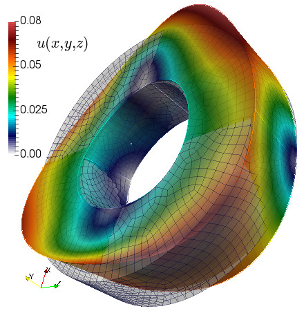
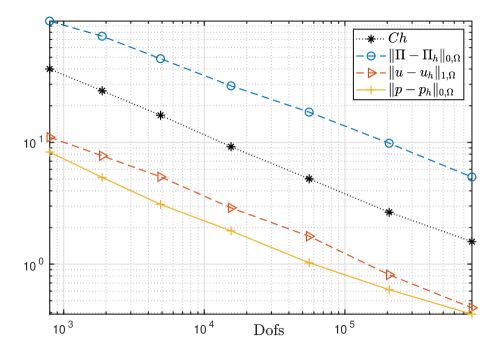
Figure 4.1: Example of approximate displacement field on the deformed domain and a coarse hexahedral mesh in the undeformed configuration (left); and error history for an accuracy test of the mixed formulation for hyperelasticity (right) generated using a lowest-order discretisation.

Before carrying out model validation and performing simulations with the fully coupled model described in Section 2, we conduct a mesh convergence test to assess the accuracy of the mixed finite element scheme proposed for the three-field hyperelasticity subproblem (2.3)-(2.4), in the case when the material is completely passive. The following test has been employed (for isotropic, Mooney-Rivlin materials) as a benchmark for different finite element solvers (Chamberland et al., 2010). In the 3D domain defined by a ring-shaped region of width 0.25 cm, internal diameter of 0.5 cm and external diameter of 1 cm, we define closed-form manufactured solutions as

$$p(x,y,z)=x^{4}-y^{4}-z^{4},\quad{\boldsymbol{u}}(x,y,z)=\biggl{(}x^{4}+\frac{2}{5}yz,\ y^{4}+\frac{2}{5}xz,\ \frac{1}{10}z^{4}-\frac{2}{5}xyz\biggr{)}^{\tt t},$$

and construct an exact form of the Kirchhoff stress, as well as body loads and eventually traction terms using these smooth functions. Sheetlets are radially defined, whereas fibres are clockwise oriented with respect to the $y$ axis, and the hyperelasticity parameters are set according to the second part of Table 3.1. Boundary conditions were considered of mixed type as in (2.11), but setting appropriate non-homogeneous terms. The traction boundary $\partial\Omega_{N}$ corresponds to the top and bottom faces of the ring (parallel to the $xz$ axis where the normal vector is ${\boldsymbol{\nu}}=(0,\pm 1,0)^{\tt t}$), whereas the normal displacement boundary $\partial\Omega_{D}$ is conformed by the internal and external curved surfaces. We compute errors between the exact solutions and the approximate fields generated by the lowest-order scheme on a sequence of unstructured hexahedral meshes of different resolutions. These (absolute) errors are measured in the tensor and scalar $L^{2}-$norms for the Kirchhoff stress and pressure, respectively; and in the $\mathbf{H}^{1}-$norm for the displacements. We plot the results versus the number of degrees of freedom in Figure 4.1(right), where we can observe an optimal convergence (first-order in this case), as anticipated in Section 3. The number of Newton iterates required to reach convergence was in average 4.

4.1 Conduction velocity assessment

Temp.	$h=0.025$ cm,$\Delta t=0.03$ ms	$h=0.0125$ cm,$\Delta t=0.0075$ ms	$h=0.006$ cm,$\Delta t=0.00125$ ms
$T=33^{\circ}$C	0.356	0.377	0.422
$T=35^{\circ}$C	0.428	0.435	0.441
$T=37^{\circ}$C	0.439	0.447	0.453
$T=39^{\circ}$C	0.442	0.450	0.448
$T=41^{\circ}$C	0.443	0.451	0.451

Table 4.1: Computed conduction velocities $[{\rm m/s}]$ according to different temperature values and spatio-temporal refinement.

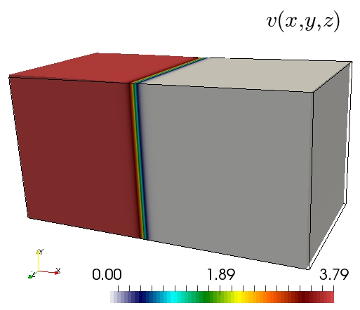
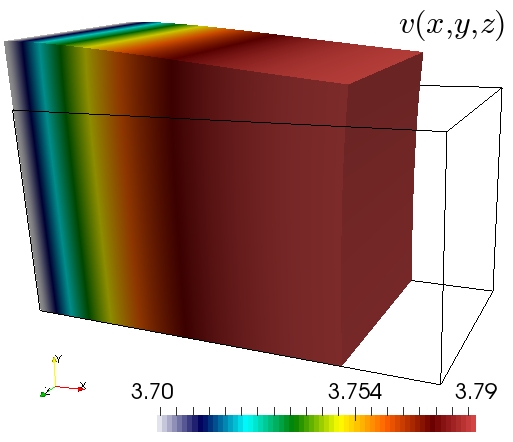
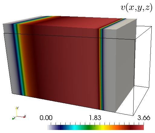
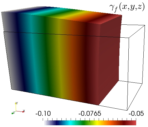
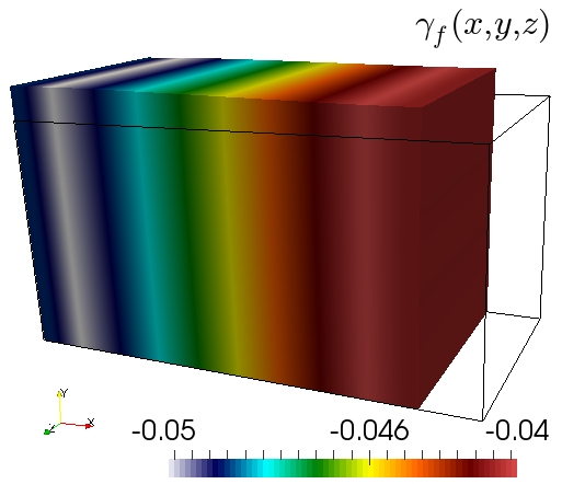
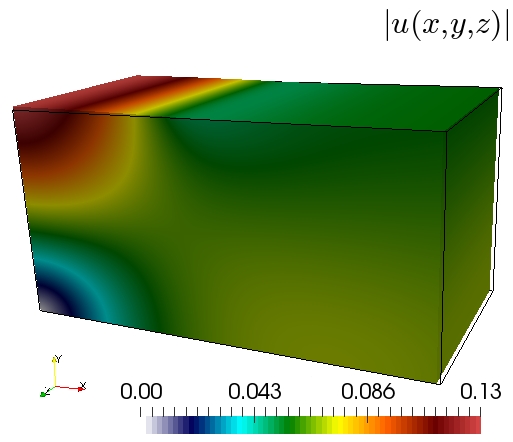
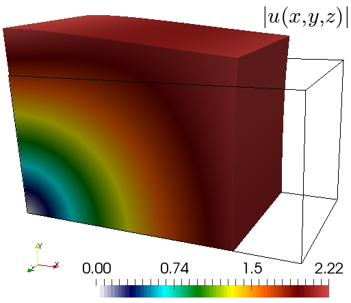
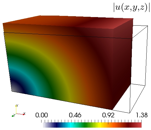
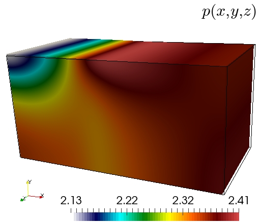
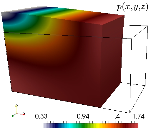
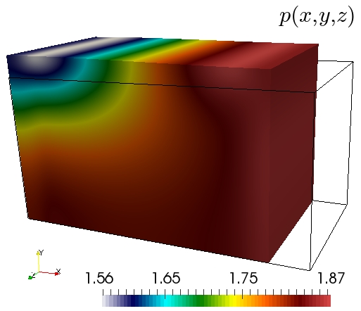
Figure 4.2: Samples of the approximate solutions (potential, activation, displacement magnitude, and solid pressure) shown on the deformed domain at $t=50,150,450$ ms (left, middle, and right panels). For this test we have used $T=39^{\circ}$C.

We next consider the electromechanical model (2.3), (2.5), (2.9) defined on the 3D slab $\Omega=(0,10)\times(0,5)\times(0,5)$ cm³. The boundary conditions correspond to (2.11) and (2.13). The bottom ($z=0$), back ($y=0$), and left ($x=0$) sides of the block will constitute $\partial\Omega_{D}$ where we impose zero normal displacements, and on the remainder of the boundary $\partial\Omega_{N}=\partial\Omega\setminus\partial\Omega_{D}$ we prescribe zero traction. We consider only constant fibre and sheet directions ${\boldsymbol{f}_{0}}=(1,0,0)^{\tt t}$, ${\boldsymbol{s}_{0}}=(0,1,0)^{\tt t}$, and a stimulus of amplitude 2 and duration 2 ms is applied on the left wall at time $t=1\,$ms, which initiates a planar wave propagation. At a temperature of $T=37^{\circ}$C, the thermo-electric effects are turned off (both $Q_{10}$ and Moore terms equal 1), and the reported maximum conduction velocity of 45.1 cm$/$s can be computed using $\tilde{D}=1.1\,$cm${}^{2}/$s (that is, setting $D_{1}=D_{2}=0$). Then, variations of temperature and of the constants that characterise the nonlinear diffusion lead to slight modifications on the conduction velocity. Here this value is computed using the approximate potential and activation times measured between the points $(x,y,z)=(4.663,2.5,2.5)$ and $(x,y,z)=(5.337,2.5,2.5)$, that is a spatial variation in the $x-$direction of $\delta x=0.674$ cm, and employing a threshold of amplitude 1. We also vary the mesh resolution and observe that the coarsest spatio-temporal discretisation that maintains conduction velocities in physiological ranges requires a meshsize of $h=0.025$ cm and a timestep of $\Delta t=0.03\,$ms. Our results are summarised in Table 4.1. We can note that for the lowest temperatures, the changes in the mesh resolution entail substantial modifications in the conduction velocity, whereas for higher temperatures the effect seems to be milder and even coarse meshes give physiological results. After computing each conduction velocity value, we have commenced another pacing cycle (with an S2 applied at $t=330$ ms), and run the simulation until $t=720$ ms. Snapshots of the potential, activation, displacement magnitude, and solid pressure are depicted in Figure 4.2, where we can observe (in particular for $t=150$ ms) a marked deformation in the sheetlet direction complying with the shortening in the fibre direction. In Figure 4.3 we plot the history of the main thermo-electric and kinematic variables on the midpoint of the line where conduction velocities are computed. We remark that the different thermal states, in addition to modifying the conduction velocity, also affect the shape and duration of the action potential wave. In agreement with the constitutive modelling, the amount of contraction is not linked to the velocity of propagation but rather to the duration of the action potential. More precisely, since the active-strain contraction is linked to the amount of tissue undergoing a certain level of voltage, it turns out that at lower temperature the action potential wave is larger (experimental evidence for this phenomenon can be found in Fenton et al., 2013), and therefore the amount of tissue undergoing contraction is larger.

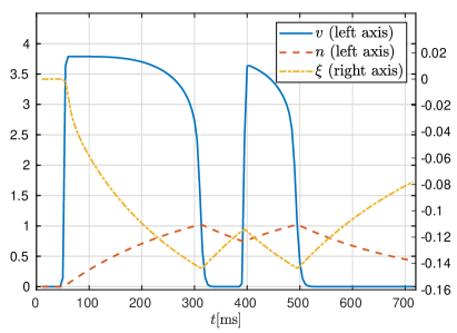
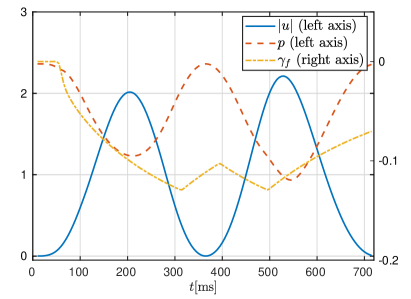
Figure 4.3: Evolution of main variables measured on the point (5,2.5,2.5) and up to $t=720$ ms, computed at temperature $T=39^{\circ}$C.

4.2 Scroll wave dynamics and localised temperature gradients

We now perform a series of tests aimed at analysing the differences in wave propagation patterns produced with different temperature conditions such as those encountered in transmural gradients induced by fever, cold/hot water, and/or localisation of other thermal sources such as ablation devices. First on the case of the base temperature $T=37^{\circ}$C, secondly in the case where the domain is subject to a temperature gradient in the direction of the sheetlets ${\boldsymbol{s}_{0}}=(0,1,0)^{\tt t}$, and third when the temperature has a radial gradient in the $xy$ plane (see Figure 4.4).

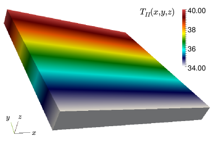
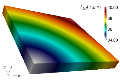
$$r=(x^{2}+y^{2})^{1/2},\,\,R=6.72\sqrt{2},$$

$$T_{II}(x,y,z)=\frac{1}{6.72}(40^{\circ}\text{C}\,y+34^{\circ}\text{C}\,(6.72-y)),\quad T_{III}(x,y,z)=\frac{1}{R}(40^{\circ}\text{C}\,r+34^{\circ}\text{C}\,(R-r)).$$

Figure 4.4: Temperature distributions in the undeformed configuration, where the colour code is in ^∘C.

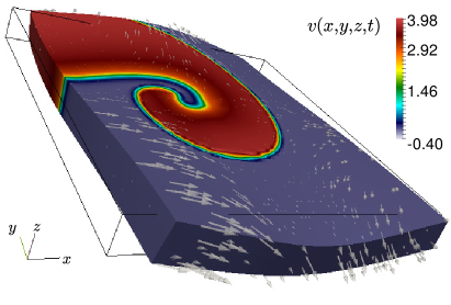
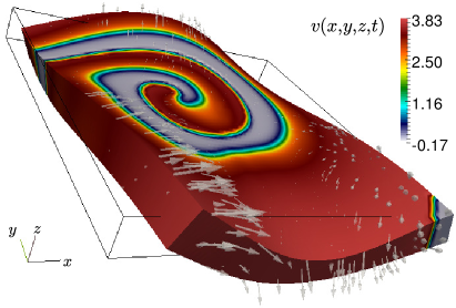
Figure 4.5: Scroll waves developed after $t=450$ ms (left panel) and $t=600$ ms (right panel) using $T=37^{\circ}$C, plotted on the deformed configuration, and where arrows indicate displacement directions.

The domain of interest is now the slab $\Omega=(0,6.72)\times(0,6.72)\times(0,0.672)$ cm³, which we discretise into a structured mesh of 72’000 hexahedral elements, with $h=0.116$ cm. We use a fixed timestep $\Delta t=0.03\,\rm ms$ and set a constant fibre direction ${\boldsymbol{f}_{0}}=(1,0,0)^{\tt t}$. We employ an S1-S2 protocol to initiate scroll waves (Bini et al., 2010), where S1 is a square wave stimulation current of amplitude 3 and duration 3  ms, starting at $t=1$  ms on the face defined by $x=0$; and S2 is a step function of the same duration and amplitude, applied on the lower left octant of the domain at $t=350\,$ ms. This time the boundary conditions for the structural problem are precisely as in (2.12), using the constant $\eta=0.05$; and the boundary conditions for the electrophysiology adopt the form (2.13). Figure 4.5 shows two snapshots of the voltage propagation through the deformed tissue slab for the first case, of constant temperature (case I). Differences between the patterns obtained at different temperatures are qualitatively shown in Figure 4.6, which displays the difference in the potential between case II and case I, as well as between case III and case I. A fourth case (not shown) was also tested, where the temperature gradient is placed in the direction of the fibres. Then the differences in propagation are much more pronounced (up to the point that the S1-S2 protocol described above is not able to produce scroll waves).

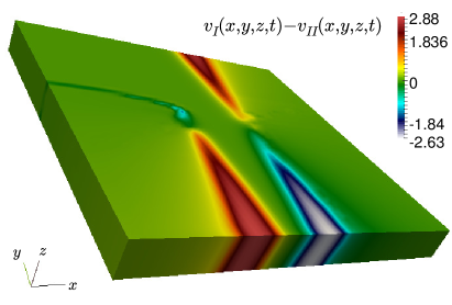
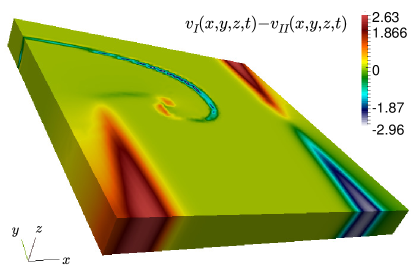
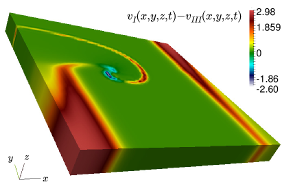
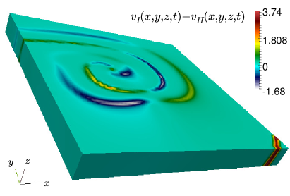
Figure 4.6: Potential difference between case I (uniform temperature at $T=37^{\circ}$C) and two different gradient distributions in the sheetlet (case II - left) and radial directions (case III - right), plotted on the reference domain at times $t=350$ ms (top panels), $t=450$ ms (middle row), and $t=600$ ms (bottom panels).

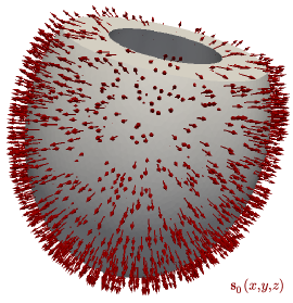
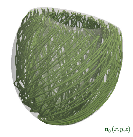
Figure 4.7: Ellipsoidal fibre distribution, collagen normal-sheetlet, and cross-fibre directions generated with a rule-based algorithm and setting $\theta_{\text{epi}}=-50^{\circ}$, $\theta_{\text{endo}}=60^{\circ}$.

4.3 Scroll waves in an idealised left-ventricular geometry

We generate the geometry of a truncated ellipsoid, as well as unstructured hexahedral meshes using GMSH (Geuzaine and Remacle, 2009). The domain has a height (base-to-apex) of 6.8 cm, a maximal equatorial diameter of 6.6 cm, a ventricular thickness of 0.5 cm at the apex and of 1.3 cm at the equator. Relatively coarse and fine partitions with 13’793 (corresponding to a meshsize of $h=0.104$ cm) and 86’264 elements (and with a meshsize of $h=0.052$ cm) are used for the simulations in this subsection. Consistently with other electromechanical simulations on idealised ventricular geometries, here we consider a time-dependent pressure distributed uniformly on the endocardium (that is, using the second relation in (2.11)). In addition, on the basal cut we impose zero normal displacements (the first condition in (2.11)), and on the epicardium we impose Robin conditions (2.12) setting a spatially varying stiffness coefficient, going linearly from $\eta_{\min}$ on the apex, to $\eta_{\max}$ on the base $\eta(y):=\frac{1}{y_{b}-y_{a}}[\eta_{\max}{(y_{b}-y)}+\eta_{\min}(y-y_{a})]$, where $y_{a},y_{b}$ denote the vertical component of the positions at the apex and base, respectively. These conditions are sufficiently general to mimic the presence of the pericardial sac (as well as the combined elastic effect of other surrounding organs) having spatially-varying stiffness.

 

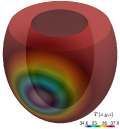
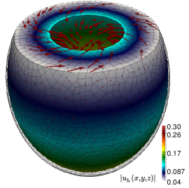
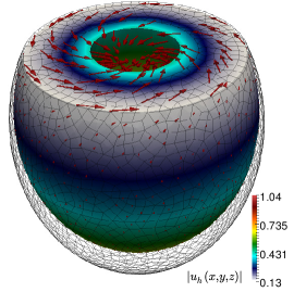
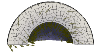
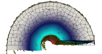
Figure 4.8: Temperature distribution for the second test case (top left), and two snapshots (200,300 ms after the S1 stimulus) illustrating the torsion and wall-thickening of the left ventricle (top centre and top right, where the arrows indicate the displacement direction). The bottom panels show cuts along the $z-$midplane for the top centre and top right figures.

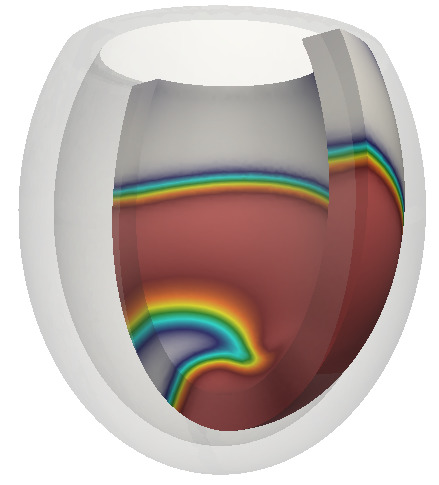
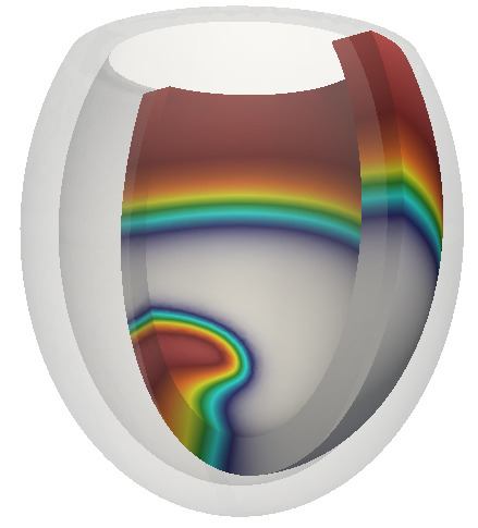
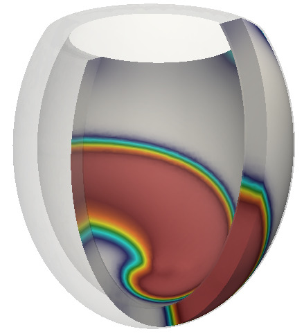
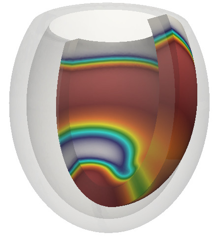
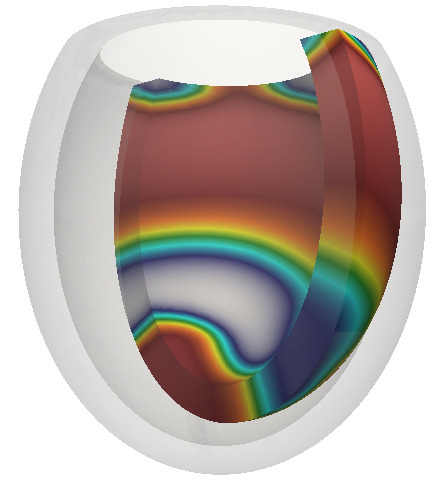
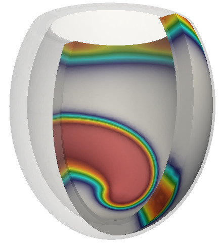
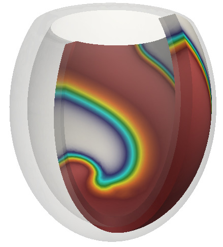
Figure 4.9: Propagation of the transmembrane potential plotted on the deformed domain, using a constant temperature (top panels) and a cold spot (bottom). Snapshots shown at 200,300,400,500 ms after the S2 stimulus.

Fibre and sheetlet directions are constructed using a slight modification to the rule-based algorithm proposed in Rossi et al. (2014), that we outline here for the sake of completeness (see Algorithm 1). The needed inputs are a unit vector ${\boldsymbol{k}_{0}}$ aligned with the centreline and pointing from apex to base, the desired maximal and minimal angles that will determine the rotational anisotropy from epicardium to endocardium, $\theta_{\text{epi}}$, $\theta_{\text{endo}}$; and boundary labels for the epicardium $\partial\Omega_{\text{epi}}$, endocardium $\partial\Omega_{\text{endo}}$, and basal cut $\partial\Omega_{\text{base}}$. The first step consists in solving the following Poisson problem (here stated in mixed form for a potential $\phi$ and a preliminary sheetlet direction ${\boldsymbol{\zeta}}$) endowed with mixed boundary conditions

$$\begin{split}-\nabla\cdot{\boldsymbol{\zeta}}&=0\quad\text{and}\quad{\boldsymbol{\zeta}}=\nabla\phi\qquad\text{in $\Omega$},\\ {\boldsymbol{\zeta}}\cdot{\boldsymbol{\nu}}&=0\quad\text{on }\partial\Omega_{\text{base}},\quad\phi=0\quad\text{on }\partial\Omega_{\text{endo}},\quad\phi=1\quad\text{on }\partial\Omega_{\text{epi}}.\end{split}$$ (4.1)

The unknowns of this problem are discretised with Brezzi-Douglas-Marini elements of first order defined on quads, and piecewise constant elements (Gatica, 2014). Once a discrete first sheetlet direction ${\boldsymbol{\zeta}}_{h}$ is computed, the final sheetlet directions are obtained by normalisation ${\boldsymbol{s}_{0}}={\boldsymbol{\zeta}}_{h}/\|{\boldsymbol{\zeta}}_{h}\|$ (all normalisations in this section refer to component-wise operations using the Euclidean norm). Secondly, we project the centreline $\widehat{{\boldsymbol{k}_{0}}}={\boldsymbol{k}_{0}}-({\boldsymbol{k}_{0}}\cdot{\boldsymbol{s}_{0}}){\boldsymbol{s}_{0}}$ and then compute an auxiliary vector field $\widehat{{\boldsymbol{f}_{0}}}$ (known as flat fibre field), using the sheetlet and the projected centreline vectors $\widehat{{\boldsymbol{f}_{0}}}={\boldsymbol{s}_{0}}\times\widehat{{\boldsymbol{k}_{0}}}/\|\widehat{{\boldsymbol{k}_{0}}}\|$. Thirdly, we proceed to project now the flat fibres onto the sheetlet planes exploiting the rotational anisotropy, through the operation

$${{\boldsymbol{f}_{0}}}=\widehat{{\boldsymbol{f}_{0}}}\cos(\theta(\phi_{h}))+{\boldsymbol{s}_{0}}\times\widehat{{\boldsymbol{f}_{0}}}\sin(\theta(\phi_{h}))+{\boldsymbol{s}_{0}}({\boldsymbol{s}_{0}}\cdot\widehat{{\boldsymbol{f}_{0}}})[1-\cos(\theta(\phi_{h}))],$$

where $\phi_{h}$ is the discrete potential and the function

$$\theta(\phi_{h}):=\frac{1}{180\pi}[(\theta_{\text{epi}}-\theta_{\text{endo}})\phi_{h}+\theta_{\text{endo}}],$$

modulates the intramural angle variation. Sample fibre, sheet and normal directions generated using this algorithm are shown in Figure 4.7.

The remaining constants employed in this Section are $\theta_{\text{epi}}=-50^{\circ}$, $\theta_{\text{endo}}=60^{\circ}$, $\eta_{\max}=0.6\,$kPa (that is, we consider a transmurally asymmetric fibre distribution), and $\eta_{\min}=0.001\,$kPa. As in the tests reported in previous subsections, the dynamics here are initiated through an S1-S2 approach (Karma, 2013), which is a standard stimulation protocol in cardiac electrophysiology (both experimentally and in silico), aimed at determining spiral wave inducibility, in the context of replicating archetypal features of cardiac arrhythmias. One typically generates a planar electrical excitation (S1), followed by a second broken stimulus (S2) during the repolarisation phase of the S1 wave, the so-called vulnerable window. In our numerical simulations, S1 is set on the apex and S2 is initiated at the same location, but only for the quadrant $x>0,z>0$.

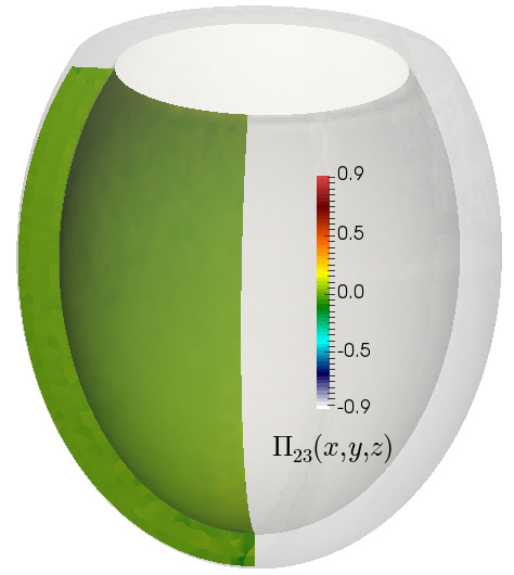
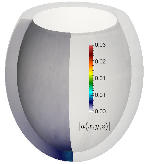
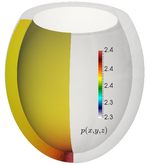
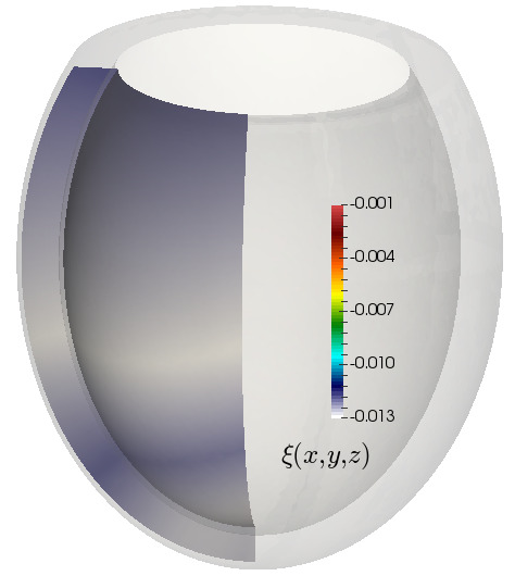
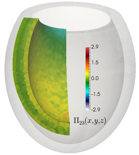
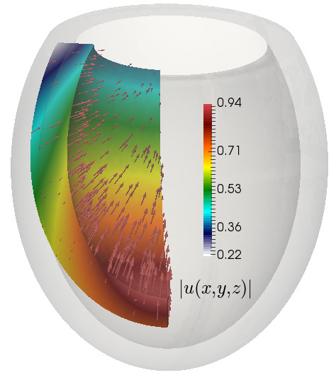
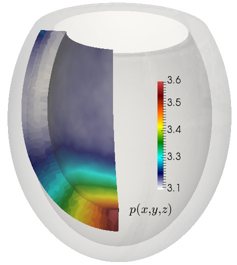
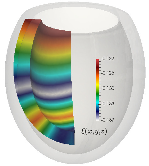
Figure 4.10: Sample approximate Kirchhoff stress, displacement, pressure, and myocyte shortening at end diastole, $t=$470 ms (top) and $t=$610 ms (bottom).

We consider two cases: one when the temperature is kept constant at $37^{\circ}$C, and another when at the time of switching on the electromechanical coupling, a localised point on the epicardium towards the base is maintained at a lower temperature $34^{\circ}$C. The temperature distribution in this second case is defined as

$$T(x,y,z)=37-3\exp(-[(x-3)^{3}+y^{2}+z^{2}]/3),$$

(see the leftmost panel in Figure 4.8). We illustrate the torsion and wall-thickening effects achieved by the orthotropic activation model in the centre and right panels of Figure 4.8, observed before applying the wave S2.

Finally, a few snapshots of the scroll wave dynamics for the two cases are presented in Figure 4.9, indicating again an important model dependency on temperature variations. In particular, the cold region notably increases the action potential duration. Once the arrhythmic pattern is fully established, the differences between the two cases are increased since higher nonlinearities appear. Samples of stress entries, displacement, pressure, and myocyte contraction are in presented in Figure 4.10, plotted on wedges that highlight ventricular thickening, stress concentrations on the endocardium, a more pronounced pressure profile near the apex, and apex to base motion. In addition to this test, we perform a set of simulations using a constant higher temperature at $39^{\circ}$C, and snapshots of the approximate potential at various time steps are displayed in Figure 4.11.

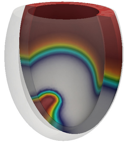
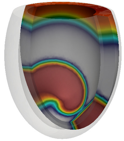
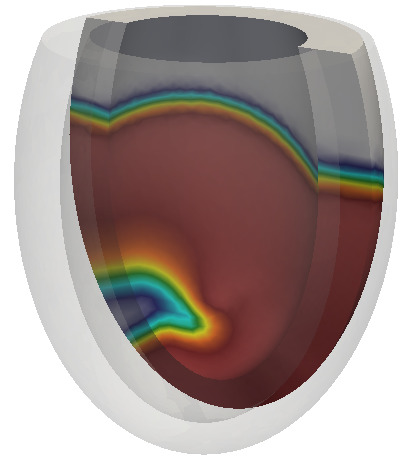
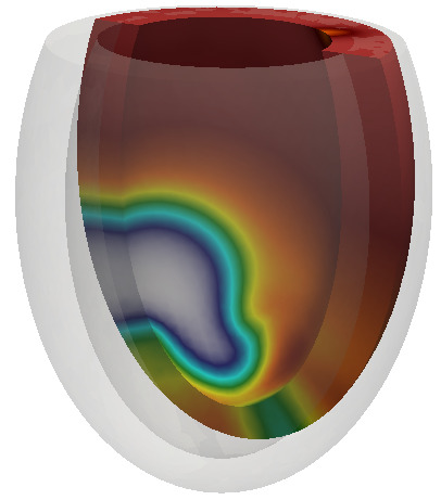
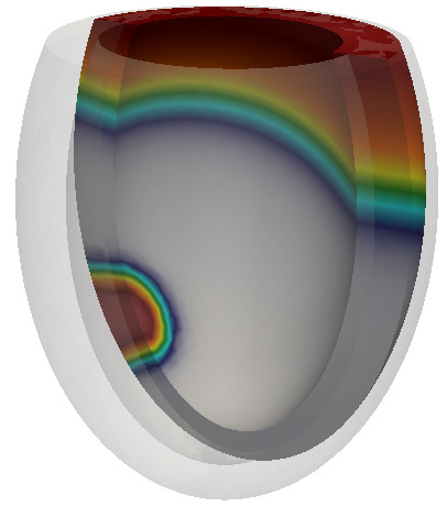
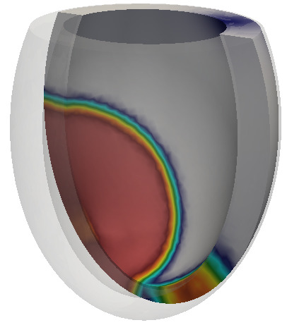
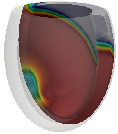
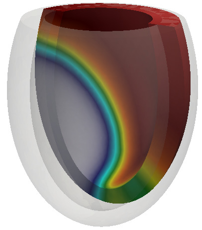
Figure 4.11: Propagation of the transmembrane potential plotted on the deformed domain, using a higher temperature throughout the domain and a thiner ventricular geometry. Snapshots shown at 100,200,…,800 ms after the S2 stimulus.

5 Concluding remarks

We have advanced a new theoretical framework for the modelling of cardiac electromechanics that incorporates active strain, anisotropic and nonlinear diffusion, and thermo-electrical coupling as main ingredients. The proposed models couple different multi-field and multi-scale (cell and sub-cell levels) phenomena, and they constitute a natural extension of porous medium electrophysiology Hurtado et al. (2016) to the case of cardiac electromechanics. The continuum homogenised approach features a temperature dependence of all reaction rates, as well as preserving material frame invariance and equilibrium constrains.

The novelties of this contribution also include a mixed-primal method based on a pressure-robust formulation for hyperelasticity. Our numerical scheme has been used to assess the influence of space and time discretisation at different thermal states in three-dimensional domains. Comparisons were made in terms of local conduction velocity as well as onset and development of scroll wave dynamics as precursors of life threatening arrhythmias. The numerical simulations demonstrated the suitability of the proposed model in reproducing key physiological features. In addition, we have observed model scalability adequate to conduct large scale computations.

Our results, collected in Section 4, suggest that the new model develops higher nonlinearities and allows for more complex fibrillation dynamics when simulating classical S1-S2 stimulation protocols in anisotropic ventricular domains. For instance, the presence of cold regions in combination with our active strain model lead to an enhanced cardiac dispersion of repolarisation, which in turn results into more involved scroll wave dynamics. Stimulation protocols (which represent the possible initiation of spiral waves and arrhythmic patterns from e.g. a fictitious ectopic focus) are greatly affected, and might even fail, under modified temperature conditions. For instance, allowing temperature gradients along or across the fibre direction can result in completely different activation patterns. A thorough computational assessment of these differences is therefore of key importance in determining experimental pacing mechanisms (Gizzi et al., 2017a). We believe that the disruptions produced uniquely by temperature gradients can be even more pronounced in the context of electromechanical simulations (as a consequence of the nonlinear coupling between the involved effects), and thus play a key role in the onset and development of arrhythmias. The set of preliminary tests presented in this paper highlights the importance of the proposed thermo-electro-mechanical coupling. Nevertheless, further investigations are necessary to determine other potential effects of the thermal coupling into the formation of local anchoring of spiral waves to material heterogeneities (pinning phenomena, Cherubini et al., 2012), their removal through low energy intra-cardiac defibrillators (unpinning protocols, see for instance Luther et al., 2011) and also the influence of the mechanochemical patterns in the induction and modulation of spatio-temporal alternans dynamics.

General limitations of our study reside in that we adopt a simplified phenomenological model for both the thermo - electrophysiology and the excitation contraction coupling. Also, we have employed only idealised geometries in all our computations, but remark that a more dedicated personalisation could be incorporated once the following list of possible generalisations are in place.

First, higher complexity in the electrophysiology and in the contraction models should be included to improve the (at this point, still quite basic) structure of the coupling mechanisms. In particular, these extensions could lead to more refined conclusions regarding the onset and control of arrhythmias and fibrillation. Secondly, it is left to investigate whether spatio-temporal variations of temperature have an effect, perhaps in long term and operating theatre scenarios. In perspective, the present study could serve in understanding and possibly controlling temperature-altered cardiac dynamics in patients subjected to whole-body hyperthermia. This is a medical procedure relevant for treating metastatic cancer and severe viral infections as e.g. HIV (Jha et al., 2016; Kinsht, 2006). Let us also remark that heat conduction in the short-scales we consider here (that is within one or two heart beats), can still be considered negligible. However, energy dissipation within an extended non-equilibrium thermodynamics framework could be an important improvement to our models. These extensions would incorporate a complete bio-heat formulation (Pennes, 1948; Gizzi et al., 2010), which can account for the combined effects of heat generation from the heart muscle, as well as advection-diffusion of temperature due to vasculature and blood flow.

Another limitation of the present model is the phenomenological description of the intracellular calcium. The lack of precise calcium dynamics forces us to include an ad hoc calcium-stretch coupling. More realistic models as the one in e.g. (Land et al., 2017) account also for better action potential shape and morphology, inter- and intracellular calcium dynamics and potentially including multiscale thermo-mechanical features; they will be incorporated in our framework in a next stage. On the same lines, we also aim at incorporating microstructure-based bidomain formulations (Richardson and Chapman, 2011), but specifically targeted for electromechanical couplings (Sharma and Roth, 2018).

In addition, we plan to apply the present model and computational methodology in the study of spatio-temporal alternans (Dupraz et al., 2015) as well as spiral pinning and unpinning phenomena (Hörning, 2012; Zhang et al., 2018). These supplementary studies would also contribute to further validate the proposed multiphysics framework against experimental evidence. In fact, the idealised ventricular domain embedded with myocardial fibres in rotational anisotropy that we used in Section 4.3 can be readily exploited towards the characterisation of the complex and unknown intramural dynamics, as soon as high-resolution imaging data are incorporated into our computational framework. A further tuning of the material parameters using synchronised endocardial and epicardial optical mapping datasets will also be carried out. These studies are considered as a direct application of the very recent technology developed in Christoph et al. (2018) for the identification of electromechanical waves, and phase singularities in particular, through advanced imaging procedures.

The passive material properties of the muscle have been considered independent of temperature, and a simple constitutive relation could be embedded in the strain-stress law using the results from Templeton et al. (1974), or in the cell contraction model following e.g. Lu et al. (2006). Moreover, taking as an example what has been proposed for other biological scenarios such as vascular pathologies, we estimate that the concepts of time-dependent mechanobiological stability (Cyron et al., 2014) as well as growth and remodelling (Cyron et al., 2016; Cyron and Humphrey, 2017), could be incorporated in the context of computational modelling of the heart. For instance, here we would consider distributed properties of collagen and muscular fibres, following for instance Pandolfi et al. (2016). Mechanoelectric feedback has been left out from this study (with the aim of isolating the effects of the thermo-electric contribution in an electromechanical context), so we could readily employ recent models for stretch activated currents (Quinn, 2015; Ward et al., 2008), or alternatively employ stress-assisted conductivity as in Cherubini et al. (2017). Other extensions include the use of geometrically detailed biventricular meshes, more sophisticate boundary conditions (setting for instance pressure-volume loops on the endocardium), and the presence of Purkinje networks (Costabal et al., 2016) and/or fast conduction systems that could definitely have an impact on the reentry dynamics. Goals in the longer term deal with optimal control problems exploiting data assimilation techniques (Barone et al., 2017) using imaging tools and in silico testing of novel defibrillation protocols (Luther et al., 2011).

Acknowledgments

This work has been partially supported by the Engineering and Physical Sciences Research Council (EPSRC) through the research grant EP/R00207X/; by the Italian National Group of Mathematical Physics (GNFM-INdAM); and by the International Center for Relativistic Astrophysics Network (ICRANet). In addition, fruitful discussions with Daniel E. Hurtado (PUC), Bishnu Lamichhane (Newcastle), Francesc Levrero (Oxford), Simone Pezzuto (USI), Adrienne Propp (Oxford), and Simone Rossi (Duke), are gratefully acknowledged. Finally, we thank the constructive criticism of two anonymous referees whose suggestions lead to several improvements with respect to the initial version of the manuscript.

References

- Alnæs et al. [2015] M. S. Alnæs, J. Blechta, J. Hake, A. Johansson, B. Kehlet, A. Logg, C. Richardson, J. Ring, M. E. Rognes, and G. N. Wells. The FEniCS project version 1.5. Archive of Numerical Software, 3(100):9–23, 2015.
- Barone et al. [2017] A. Barone, F. H. Fenton, and A. Veneziani. Numerical sensitivity analysis of a variational data assimilation procedure for cardiac conductivities. Chaos: An Interdisciplinary Journal of Nonlinear Science, 27:093930, 2017.
- Bini et al. [2010] D. Bini, C. Cherubini, S. Filippi, A. Gizzi, and P. E. Ricci. On spiral waves arising in natural systems. Communications in Computational Physics, 8:610, 2010.
- Bueno-Orovio et al. [2008] A. Bueno-Orovio, E. M. Cherry, and F. H. Fenton. Minimal model for human ventricular action potentials in tissue. Journal of Theoretical Biology, 7:544–560, 2008.
- Chamberland et al. [2010] É. Chamberland, A. Fortin, and M. Fortin. Comparison of the performance of some finite element discretizations for large deformation elasticity problems. Computers & Structures, 88(11):664–673, 2010.
- Chavan et al. [2007] K. S. Chavan, B. P. Lamichhane, and B. I. Wohlmuth. Locking-free finite element methods for linear and nonlinear elasticity in 2D and 3D. Computer Methods in Applied Mechanics and Engineering, 196:4075–4086, 2007.
- Cherubini et al. [2012] C. Cherubini, S. Filippi, and A. Gizzi. Electroelastic unpinning of rotating vortices in biological excitable media. Physical Review E, 85:031915, 2012.
- Cherubini et al. [2017] C. Cherubini, S. Filippi, A. Gizzi, and R. Ruiz-Baier. A note on stress-driven anisotropic diffusion and its role in active deformable media. Journal of Theoretical Biology, 430:221–228, 2017.
- Christoph et al. [2018] J. Christoph, M. Chebbok, C. Richter, J. Schröder-Schetelig, P. Bittihn, S. Stein, I. Uzelac, F.H. Fenton, G. Hasenfuss, Jr. Gilmour, R.F., and S. Luther. Electromechanical vortex filaments during cardiac fibrillation. Nature, 555(7698):667–672, 2018.
- Collet et al. [2017] A. Collet, J. Bragard, and P. C. Dauby. Temperature, geometry, and bifurcations in the numerical modeling of the cardiac mechano-electric feedback. Chaos: An Interdisciplinary Journal of Nonlinear Science, 27(9):093924, 2017.
- Colli Franzone et al. [2016] P. Colli Franzone, L. F. Pavarino, and S. Scacchi. Bioelectrical effects of mechanical feedbacks in a strongly coupled cardiac electro-mechanical model. Mathematical Models and Methods in Applied Sciences, 26(01):27–57, 2016.
- Costabal et al. [2016] F. S. Costabal, D. E. Hurtado, and E. Kuhl. Generating purkinje networks in the human heart. Journal of Biomechanics, 49:2455–2465, 2016.
- Cyron and Humphrey [2017] C. J. Cyron and J. D. Humphrey. Growth and remodeling of load-bearing biological soft tissues. Meccanica, 52:645–664, 2017.
- Cyron et al. [2014] C. J. Cyron, J. S. Wilson, and J. D. Humphrey. Mechanobiological stability: a new paradigm to understand the enlargement of aneurysms? Journal of the Royal Society Interface, 11:20140680, 2014.
- Cyron et al. [2016] C. J. Cyron, R. C. Aydin, and J. D. Humphrey. A homogenized constrained mixture (and mechanical analog) model for growth and remodeling of soft tissue. Biomechanical Modeling in Mechanobiology, 15:1389–1403, 2016.
- Dupraz et al. [2015] M. Dupraz, S. Filippi, A. Gizzi, A. Quarteroni, and R. Ruiz-Baier. Finite element and finite volume-element simulation of pseudo-ECGs and cardiac alternans. Mathematical Methods in the Applied Sciences, 38(6):1046–1058, 2015.
- Eisner et al. [2017] D. A. Eisner, J. L. Caldwell, K. Kistamás, and A. W. Trafford. Calcium and excitation-contraction coupling in the heart. Circulation Research, 121(2):181–195, 2017.
- Fenton and Karma [1998] F. H. Fenton and A. Karma. Vortex dynamics in three-dimensional continuous myocardium with fiber rotation: Filament instability and fibrillation. Chaos, 8:20–47, 1998.
- Fenton et al. [2013] F. H. Fenton, A. Gizzi, C. Cherubini, N. Pomella, and S. Filippi. Role of temperature on nonlinear cardiac dynamics. Physical Review E, 87:042709, 2013.
- Filippi et al. [2014] S. Filippi, A. Gizzi, C. Cherubini, S. Luther, and F. H. Fenton. Mechanistic insights into hypothermic ventricular fibrillation: the role of temperature and tissue size. Europace, 16:424–434, 2014.
- Gatica [2014] G. N. Gatica. A Simple Introduction to the Mixed Finite Element Method. Theory and Applications. Springer-Verlag, Berlin, 2014.
- Geuzaine and Remacle [2009] C. Geuzaine and J.-F. Remacle. Gmsh: A 3-D finite element mesh generator with built-in pre- and post-processing facilities. International Journal for Numerical Methods in Engineering, 79:1309–1331, 2009.
- Gizzi et al. [2010] A. Gizzi, C. Cherubini, S. Migliori, R. Alloni, R. Portuesi, and S. Filippi. On the electrical intestine turbulence induced by temperature changes. Physical Biology, 7:016011, 2010.
- Gizzi et al. [2017a] A. Gizzi, A. Loppini, E. M. Cherry, C. Cherubini, F. H. Fenton, and S. Filippi. Multi-band decomposition analysis: Application to cardiac alternans as a function of temperature. Physiological Measurements, 38:833–847, 2017a.
- Gizzi et al. [2017b] A. Gizzi, A. Loppini, R. Ruiz-Baier, A. Ippolito, A. Camassa, A. La Camera, E. Emmi, L. Di Perna, V. Garofalo, C. Cherubini, and S. Filippi. Nonlinear diffusion & thermo-electric coupling in a two-variable model of cardiac action potential. Chaos: An Interdisciplinary Journal of Nonlinear Science, 27:093919, 2017b.
- Hill and Sec [1938] A. V. Hill and R. S. Sec. The heat of shortening and the dynamic constants of muscle. Proceedings of the Royal Society of London B: Biological Sciences, 126:136–195, 1938.
- Holzapfel and Ogden [2009] G. A. Holzapfel and R. W. Ogden. Constitutive modelling of passive myocardium: a structurally based framework for material characterization. Philosophical Transactions of the Royal Society of London A: Mathematical, Physical and Engineering Sciences, 367:3445–3475, 2009.
- Hörning [2012] M. Hörning. Termination of pinned vortices by high-frequency wave trains in heartlike excitable media with anisotropic fiber orientation. Physical Review E, 86:031912, 2012.
- Hurtado et al. [2016] D. E. Hurtado, S. Castro, and A. Gizzi. Computational modeling of non-linear diffusion in cardiac electrophysiology: A novel porous-medium approach. Computer Methods in Applied Mechanics and Engineering, 300:70–83, 2016.
- Jha et al. [2016] S. Jha, P. K. Sharma, and R. Malviya. Hyperthermia: Role and risk factor for cancer treatment. Achievements in the Life Sciences, 10:161–167, 2016.
- Karma [1994] A. Karma. Electrical alternans and spiral wave breakup in cardiac tissue. Chaos: An Interdisciplinary Journal of Nonlinear Science, 4:461–472, 1994.
- Karma [2013] A. Karma. Physics of cardiac arrhythmogenesis. Annual Review of Condensed Matter Physics, 4:313—337, 2013.
- Kienast et al. [2017] R. Kienast, M. Handler, M. Stöger, D. Baumgarten, F. Hanser, and C. Baumgartner. Modeling hypothermia induced effects for the heterogeneous ventricular tissue from cellular level to the impact on the ECG. PLOS ONE, 12(8):1–22, 08 2017.
- Kinsht [2006] D. N. Kinsht. Modeling of heat transfer in whole-body hyperthermia. Biophysics, 51:659–663, 2006.
- Land et al. [2017] S. Land, S.-J. Park-Holohan, N. P. Smith, C. G. dos Remedios, J. C. Kentish, and S. A. Niederer. A model of cardiac contraction based on novel measurements of tension development in human cardiomyocytes. Journal of Molecular and Cellular Cardiology, 106(Supplement C):68–83, 2017.
- Lawton [1954] R. W. Lawton. The thermoelastic behavior of isolated aortic strips of the dog. Circulation Research, 2:344–353, 1954.
- Lee et al. [2009] J. Lee, S. Niederer, D. Nordsletten, I. Le Grice, B. Smail, D. Kay, and N. Smith. Coupling contraction, excitation, ventricular and coronary blood flow across scale and physics in the heart. Phil. Trans. Roy. Soc. London A, 367:2311–2331, 2009.
- Lu et al. [2006] X. Lu, L. S. Tobacman, and M. Kawai. Temperature-dependence of isometric tension and cross-bridge kinetics of cardiac muscle fibers reconstituted with a tropomyosin internal deletion mutant. Biophysical Journal, 91(11):4230–4240, 2006. ISSN 0006-3495.
- Luther et al. [2011] S. Luther, F. H. Fenton, and et. al. Low-energy control of electrical turbulence in the heart. Nature, 475:235–239, 2011.
- Nash and Hunter [2000] M. P. Nash and P. J. Hunter. Computational mechanics of the heart. Journal of Elasticity, 61:113–141, 2000.
- Nobile et al. [2012] F. Nobile, R. Ruiz-Baier, and A. Quarteroni. An active strain electromechanical model for cardiac tissue. International Journal for Numerical Methods in Biomedical Engineering, 28:52–71, 2012.
- Pandolfi et al. [2016] A. Pandolfi, A. Gizzi, and M. Vasta. Coupled electro-mechanical models of fiber-distributed active tissues. Journal of Biomechanics, 49:2436–2444, 2016.
- Pennes [1948] H. H. Pennes. Analysis of tissue and arterial blood temperatures in the resting human forearm. Journal of Applied Physiology, 1:93–122, 1948.
- Pezzuto et al. [2014] S. Pezzuto, D. Ambrosi, and A. Quarteroni. An orthotropic active-strain model for the myocardium mechanics and its numerical approximation. European Journal of Mechanics - A/Solids, 48:83–96, 2014.
- Propp et al. [2018] A. Propp, A. Gizzi, F. Levrero-Florencio, and R. Ruiz-Baier. An orthotropic electro-viscoelastic model for the heart with stress-assisted diffusion. Preprint available from http://people.maths.ox.ac.uk/ruizbaier, 2018.
- Qu et al. [2014] Z. Qu, G. Hu, A. Garfinkel, and J. N. Weiss. Nonlinear and stochastic dynamics in the heart. Physics Reports, 543:61–162, 2014.
- Quarteroni et al. [2017] A. Quarteroni, T. Lassila, S. Rossi, and R. Ruiz-Baier. Integrated heart – coupled multiscale and multiphysics models for the simulation of the cardiac function. Computer Methods in Applied Mechanics and Engineering, 314:345–407, 2017.
- Quinn [2015] T. A. Quinn. Cardiac mechano-electric coupling: a role in regulating normal function of the heart? Cardiovascular Research, 108:1–3, 2015.
- Richardson and Chapman [2011] G. Richardson and S.J. Chapman. Derivation of the bidomain equations for a beating heart with a general microstructure. SIAM J. Appl. Math., 71:657–675, 2011.
- Rossi et al. [2014] S. Rossi, T. Lassila, R. Ruiz-Baier, A. Sequeira, and A. Quarteroni. Thermodynamically consistent orthotropic activation model capturing ventricular systolic wall thickening in cardiac electromechanics. European Journal of Mechanics: A/Solids, 48:129–142, 2014.
- Ruiz-Baier [2015] R. Ruiz-Baier. Primal-mixed formulations for reaction-diffusion systems on deforming domains. Journal of Computational Physics, 299:320–338, 2015.
- Sharma and Roth [2018] K. Sharma and B. J. Roth. The mechanical bidomain model of cardiac muscle with curving fibers. Physical Biology, 15(066012), 2018.
- Spencer [1989] A. J. M. Spencer. Continuum Mechanics. Longman Group Ltd, London, 1989.
- Sugi and Pollack [1998] H. Sugi and G. H. Pollack. Mechanisms of work production and work absorption in muscle, volume Advances in Experimental Medicine and Biology. Springer, 1998.
- Templeton et al. [1974] G. H. Templeton, K. Wildenthal, J. T. Willerson, and W. C. Reardon. Influence of temperature on the mechanical properties of cardiac muscle. Circulation Research, 34(5):624–634, 1974.
- Trayanova and Rice [2011] N. A. Trayanova and J. J. Rice. Cardiac electromechanical models: from cell to organ. Frontiers in Physiology, 2:43, 2011.
- Vazquez [2006] J. L. Vazquez. The Porous Medium Equation: Mathematical Theory. Oxford Mathematical Monographs, 2006.
- Ward et al. [2008] M.-L. Ward, I. A. Williams, I. Chu, P. J. Cooper, Y. K. Ju, and D. G. Allen. Stretch-activated channels in the heart: Contributions to length-dependence and to cardiomyopathy. Progress in Biophysics and Molecular Biology, 97:232–249, 2008.
- Weinberg et al. [2017] S. H. Weinberg, D. B. Mair, and C. A Lemmon. Mechanotransduction dynamics at the cell-matrix interface. Biophysical Journal, 112:1962–1974, 2017.
- Wilson and Crandall [2011] T. E. Wilson and C. G. Crandall. Effect of thermal stress on cardiac function. Exercise and Sport Sciences Reviews, 39(1):12–17, 2011.
- Zhang et al. [2018] J. Zhang, J. Tang, J. Ma, J. M. Luo, and X. Q. Yang. The dynamics of spiral tip adjacent to inhomogeneity in cardiac tissue. Physica A: Statistical Mechanics and its Applications, 491:340–346, 2018.