capbtabboxtable[][\FBwidth]
From the Periphery to the Center:
Information Brokerage in an Evolving Network
Abstract
Interpersonal ties are pivotal to individual efficacy, status and performance in an agent society. This paper explores three important and interrelated themes in social network theory: the center/periphery partition of the network; network dynamics; and social integration of newcomers. We tackle the question: How would a newcomer harness information brokerage to integrate into a dynamic network going from periphery to center? We model integration as the interplay between the newcomer and the dynamics network and capture information brokerage using a process of relationship building. We analyze theoretical guarantees for the newcomer to reach the center through tactics; proving that a winning tactic always exists for certain types of network dynamics. We then propose three tactics and show their superior performance over alternative methods on four real-world datasets and four network models. In general, our tactics place the newcomer to the center by adding very few new edges on dynamic networks with nodes.
1 Introduction
An agent society (or system) is defined by patterns of dyadic links between individuals. Research on social networks has greatly advanced our understanding of how traits such as ties, modules, and flow, impact agents’ positions [4]. Gaining a central position is seen as beneficial thanks to the relative easiness it brings to receive diverse information and exercise influence over other agents, i.e., a central position defines an information broker who accesses and integrates information through social links. This notion has wide implications on roles, status and leadership in organizations [20] and has recently facilitated applications such as IoT [10] and semantic web [13].
A predominant meso-scale feature of many complex networks is the emergence of tiers: Sitting at the center is a densely-connected cohesive core, and on the outskirts a loosely-knit periphery. This paper asks the question: How would a newcomer harness information brokerage to integrate into a dynamic network going from the periphery to the center? Two assumptions are made: (a) We focus on networks that have a distinguished center, e.g., a core/periphery structure; and (b) We examine the decisions and processes of relationships building. The aim is to approach the question through a formal, algorithmic lens. This demands settling two issues: (1) The first concerns representations of center and brokerage. We stay consistent with the framework defined in [21] and treats information brokers as agents that give the newcomer low eccentricity, hence getting into the (Jordan) center of the network [26]. (2) The second is about network dynamics. As the network evolves with time, the model must make sense for dynamic networks. This sets this work apart from previous works on information brokerage where only static networks are of concern and brings extra complications to the problem. Even though we phrase the problem assuming additive changes to the network (as, e.g., a citation network), our notions and techniques also apply to fully dynamic networks.
Contribution.
(1) We formulate integration as repeated, parallel interplays between a newcomer and the ensemble of other agents in the network it aims to join. The network evolves in the form of a sequence of snapshots in discrete time, which is determined by the initial network, the network’s own evolution trace, and the newcomer’s strategy for adding ties. The goal of the newcomer is to adopt a tactic that moves it from periphery to center within a finite number of steps regardless of dynamic changes of the network. (2) We study the existence of such strategies under certain reasonable conditions. In particular, when the center is bounded – as in many networks with a center/periphery structure – the newcomer has a winning tactic. (3) We propose three simple tactics and compare them with two methods from [21] which are designed for the same problem on static networks. Our tactics outperform the alternatives over four real-world dynamic networks.We also propose four dynamic network models with varying core/periphery-ness: dynamic preferential attachment, Jackson-Rogers, rich-club and onion models, and analyze the performance of tactics over them. Our tactics bring the newcomer to the center by creating less than 10 new edges in all of the experiments performed.
Related work.
We focus on the individual strategies on networks with dynamic core periphery structure, which related to three categories: core-periphery structure, network building problem. Game-theoretical research on network formation focuses on equilibria among rational agents [14, 6]; in contrast, our paper complements this body of work by investigating optimal tactics for a single agent in a dynamic setting. Motivated from [25], [21] initiates the static version of the problem under investigation, namely, building the least amount of edges to bring a newcomer to the network center. We build on their work and study dynamic networks. As opposed to the static case, a desired tactic may not exist under certain forms of network dynamics.
The definition of a graph center goes back to the work of Jordan in the 19th century and eccentricity belongs to a family of distance-based centrality indices [3]. Despite its simplicity, eccentricity has been useful in many places, e.g. from analyzing islands networks [hage1995eccentricity] and the rise of the Medici family in marriage alliance network [22] to mapping Hollywood actors/actresses [11]. Although the center can be identified for any network, we specifically target at core/periphery structures [2]. Observations of such tiered structures root in economics where the world is divided between industrial, “core” nations and agricultural, “peripheral” nations [snyder1979structural, 17]. Similar structures are subsequently witnessed in, e.g., social networks [7], scientific citation [doreian1985structural], and trading networks [9]. Agents in the core, being hubs, enjoy many benefits such as control over information and domination of resources. A crucial feature of the core, apart from its central position and density, is the stability over time [8, 24].
2 Network Building in a Dynamic Network
A social network is an undirected graph ; is a set of vertices (or agents), an edge , denoted by , represents links between agents . The distance is the shortest length of any path between and ; for , set . The eccentricity of is . The radius and diameter of are, resp., and [11]. The center of is the set .
A dynamic network evolves in discrete-time, i.e., it consists of a (potentially infinite) list of networks where is the network instance at timestamp . We define the set of vertices of a dynamic network as the set . As may contain infinitely many timestamps, may be infinite. For any , the set of neighbors is . As individuals usually have an only bounded capacity to manage social links, we require that being finite for all . Thus the graph stays a locally-finite graph.
Two caveats exist: Firstly, we should clarify what forms of structural changes may happen. In principle, any addition/removal of vertices/edges may occur. For the majority of this paper, however, we focus on a simpler form of dynamics where the network only makes additive changes,i.e., the only allowable updates are the addition of vertices/edges. Secondly, we need a policy regarding the frequency of timestamps. One natural method is to separate consecutive instances with a fixed period, e.g., instances of a social network may be generated by day. Another common approach is to add a timestamp only when an update occurs, e.g., a timestamp may correspond to when certain update happens between two individuals causing a new edge to form. The exact meaning of a timestamp should be up to the actual application scenario.
We study the process that expands a network with new edges. Imagine an outside agent who aims to integrate into the network and explore information within. Information brokers refer to a set of appropriately located vertices who collectively give the newcomer good access to the information within the network. More formally, for , ( may or may not overlap), denotes the network . Throughout, we use to denote a newcomer. For any subset , define as . Thus is the resulting network obtained after integrating into via building links between and every vertex in . The following definition is proposed by [21].
Definition 1.
A broker set for is such that .
The intuition behind the definition is that by making contacts with members of a broker set, can gain maximum access to the network. As a broker set always exists for a graph , the question then focuses on the size of broker sets. The minimum broker set problem asks for a broker set with the smallest cardinality and is shown to be NP-complete [21].
The main goal of this paper is to extend the above notions to a dynamic setting, capturing the process in which a newcomer builds ties with an evolving network to gain maximal access of information in the network. Note that connecting to brokers embodies a dynamic process: As building relations requires effort and time, a broker set is built iteratively where edges are added for one by one, until its eccentricity becomes . Over a dynamic network , would act while the network evolves [28]. From ’s perspective, its position relies not only on its own actions but also on the ensemble of all other agents in the network. At any timestamp, both parties make moves simultaneously, affecting the next network instance. Agent ’s move consists of building new edges to the current graph; the others party’s move consists of updates of the form “adding a new edge (either between two existing nodes, or a new vertex and an existing node)”. Formally, for any network , an expansion of is a network whose every connected component contains at least one node in , i.e., is a network achieved by the two types of updates.
Definition 2.
Fix an initial network and a newcomer . For , an integration process (IP) is a dynamic network where
where is a set of vertices in that are not adjacent to , and is an expansion of that does not contain .
Conceptually, one can view an IP as an iterative interplay between and the network who acts as a sort of “opponent”. Progressing from iteration to the network changes by (i) “attaching” a subgraph ; this may bring more vertices and edges to ; and (ii) adding an edge between and all vertices in . The sequence of edges is called the evolution trace and the sequence of sets is called the newcomer strategy of . The IP is uniquely determined by the initial network , actions of the network (in the form of an evolution trace) and the actions of (in the form of a newcomer strategy). The definition of a dynamic network means that an IP must satisfy a locally-finiteness (LF) condition:
(LF) Any agent (including ) eventually stops adding new edges, i.e., does not appear in the network .
3 Information Broker in a Dynamic Network
A question arises as to how the newcomer may choose its strategy during an IP to get into the network center.
Definition 3.
An IP is a broker scheme of if for some .
We are interested in tactics that construct a broker scheme regardless of the evolution trace. Here, our attention is on a type of strategies where makes decisions about at each timestamp given only the current network instance .
Definition 4.
A tactic of is a function defined on the set of all networks such that for any and . An IP is said to be consistent with if its newcomer strategy satisfies that ; we use to denote the class of all IPs consistent with .
We generalize information brokerage to the dynamic context.
Definition 5.
Let be a collection of IPs. A broker tactic for is a tactic such that and any is a broker scheme.
The rest of the section studies the existence of broker tactics.
Definition 6.
Fix numbers and . An IP is -confined if of the evolution trace contains at most and any for all .
-confined IP is static where broker tactics always exist.
Theorem 1.
For any , there exists a broker tactic of for the class of -confined IPs.
Proof.
Define the tactic of as follows: Let be an arbitrary set of vertices in not adjacent to (or the set of all vertices not adjacent to if more than such vertices exist). We claim that any IP consistent with is a broker scheme of . Since , for any timestamp , the network instance contains at most one vertex not-linked to . Moreover, if is linked to all other vertices in , and then is a broker scheme.
Now suppose that for all , the evolution process adds a new vertex, say and an edge where . Then there must be a timestamp , such that for some , as otherwise some vertex in will have an infinite degree. In the instance , the furthest vertex from is with and hence . Clearly, is not connected to all vertices in and thus . Therefore at this timestamp, , and the IP is a broker scheme. ∎
Theorem 2.
No broker tactic exists for the set of -confined IPs when .
Proof.
Take a tactic of . Inductively construct -confined IP in where for any : Suppose at instance . Consider the graph . If is not adjacent to any vertex in , then clearly will not reach the center of regardless of . Otherwise, take that is the furthest from . Let . Let be a simple path attaches to at one end, do not belong to , and the edges are . Now set .
Clearly, as the furthest vertex from is . Now pick a path between and , and let be the vertex along this path that is adjacent to ; , and for all other vertices , . As , . This means that . ∎
One can view as specification of an IP protocol: When , the newcomer gains an upper hand to reach the center; If, on the other hand, , may never “catch up” with the rest of the network. The only case left is when , and we will focus on this case in our experiments.
To further investigate the existence of a broker tactic, we look closely at the proof of Thm. 1. The non-existence of a broker tactic is due to the fact that the center “shifts” as new vertices are added. This may not be the case in real-life, e.g., a core/periphery structure contains a highly stable network core meaning that the network center would be relatively stable [8, 24].
Definition 7.
Let be a dynamic network. We say that has a bounded center if there exists a vertex , and such that .
Bounded center property means that the center of the dynamic network would not expand or shift indefinitely. The following fact easily follows from (LF).
Lemma 1.
is a dynamic network with a bounded center if and only if the set is a finite set.
Proof.
Suppose is finite. Pick any and set as ; must be in as is finite. Therefore .
Conversely, suppose has a bounded center. Then is a subset of the union where each , . Clearly, . Suppose is a finite set, by (LF), is also finite. Therefore, is also finite, and hence is finite. ∎
Theorem 3.
There exists a broker tactic for the class of all -confined IPs with a bounded center.
Proof.
Define tactic by where and if such a vertex exists; otherwise. To show that there is some that has a bounded center, simply take and evolution trace where the edges in each are , . The corresponding IP will set . Clearly after timestamp 3 when all edges are added, and for all .
Take an IP with a bounded center. By Lem. 1, is finite. By (LF), the set is also finite. Thus for some timestamp , all edges where would have been added to . At this timestamp, belongs to and the IP is a broker scheme. ∎
4 Cost-Effective Tactics and Evaluations
As shown empirically below, real networks usually have bounded centers, but the tactic in the proof of Thm. 3 is unpractical as it may create arbitrarily many edges. To fix a framework where tactics are comparable, from now on, we focus on tactics that add a single edge in a timestamp (i.e., ) until enters . By the cost of an IP, we mean the number of timestamps elapsed before enters the center (infinite if never enters the center). We are interested in cost-effective tactics that result in the least expected cost.
Uset-based tactics.
Over static networks, our problem reduces to finding a minimum broker set. The problem is shown to be NP-complete by [21] who also gave several cost-effective tactics. At any timestamp of , the uncovered set (Uset) is . Two tactics, named and resp., add an edge from to a vertex that has maximum degree (as in ) or betweenness (as in ) centrality. Over static networks, their tactics build a sub-radius dominating set which corresponds to a broker set and is normally small, e.g., finds a broker set of size 4 on a (static) collaboration network with vertices.
Rset-based tactics.
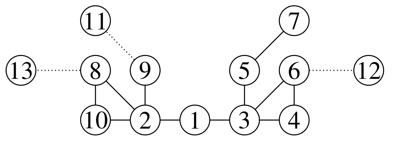
A downside, however, lies with the Uset-based tactics over core/periphery structures: Once a link is created from to someone in the core, these tactics would forbid further links with those that are also in the core (as they are “covered”). As a result, they result in suboptimal solutions. We thus modify the method by allowing to link with some vertices in the Uset, as long as they are close to uncovered vertices. More formally, we define a remote-center set (Rset) at timestamp of as , where is a furthest vertex from . We introduce and as tactics that, instead of choosing vertices from at timestamp , links with a in the Rset that has the largest degree (in ) or maximum betweenness (in ) centrality. To contrast these tactics, Fig. 1 shows an example where gave suboptimal solutions for both static/dynamic case; gave an optimal solution for static but not for the dynamic case; and / gave optimal solutions for both cases.
MUF.
Another tactic for is to link with neighbors of a center vertex , thus getting into the center. To minimize cost, is chosen to have the least degree in . A heuristic then selects from the most useful friends (MUF) of , which are defined as neighbors of that are at distance from the furthest vertex from . Alg.1 implements this tactic for one timestamp (when ). This tactic will work in dynamic networks whose center does not change much.
We run and evaluate the tactics on 4 real-world datasets.
Datasets.
The number of timestamps in these networks ranges from 50 to .
- CollegeMsg network (Msg)
-
is a timestamped online social network at the University of California, Irvine [23]; An edge denotes a message sent between and .
- Bitcoin OTC trust network (Bitcoin)
-
record anonymous Bitcoin trading on Bitcoin OTC with temporal information [18]. An edge denotes a trade between and .
- Cit-HepPh network (Cit)
-
is a high-energy physics citation network [19], which collects all papers from 1992 to 1998 on arXiv; An (undirected) edge denotes that paper cites paper .
- Trade network (Trade)
-
denotes yearly world trade partnership, 1951 – 2009 [15]; Edges represent trade partnership which is defined based on import/export between two countries.
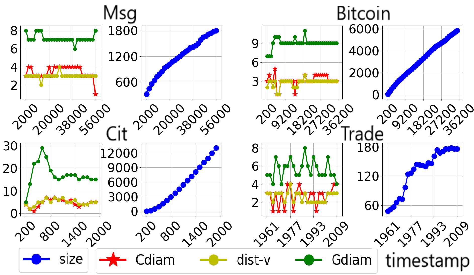
All networks above, apart from Trade, has only additive changes to the network. Table 1 shows multiple statistics of the last networks instance. The goodness of fit shows how well nodal degrees align with a power-law distribution, indicating a clear scale-free property. clus-coef and diam show that the networks have high clustering coefficient and low diameter, indicating small-world property. Cp-coef is a metrics for core-periphery structure; a positive value indicates a clear core/periphery structure [12]. Fig. 2 analyzes temporal properties of the networks. It is clearly seen that, despite the continuous expansion of the network (in size), the graph center gains little in terms of diameter. Moreover, the location of the center does not shift as the maximum distance between a fixed vertex and vertices in the center stay bounded by a small distance during all timestamps.
| Trade | Msg | Bitcoin | Cit | |
| 176 | 1899 | 5875 | 14083 | |
| 1229 | 20296 | 21489 | 104211 | |
| clust-coef | 0.54 | 0.10 | 0.17 | 0.26 |
| max.deg | 113 | 255 | 795 | 266 |
| diam | 4 | 8 | 9 | 15 |
| center size | 118 | 1 | 16 | 61 |
| timestamps | 50 | 59835 | 35592 | 2000 |
| goodness of fit | 0.74 | 0.89 | 0.86 | 0.91 |
| cp-coef | 0.11 | 0.08 | 0.11 | 0.14 |
Experiment 1 (Cost).
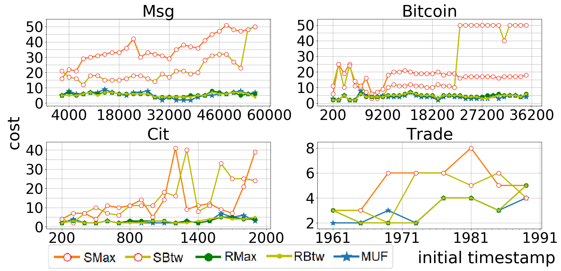
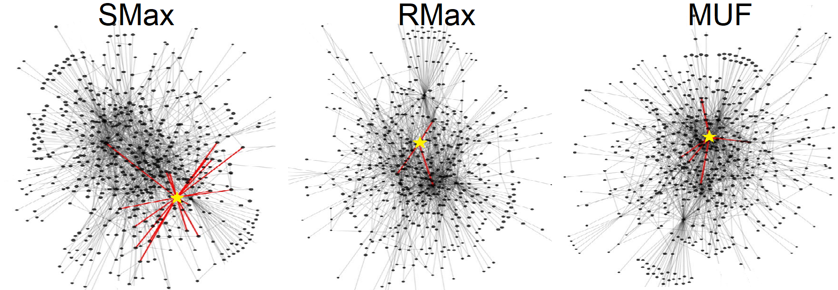
The goal is to compare the tactics treating / as benchmarks. For each dataset, we choose 28(Msg), 36(Bitcoin), 18(Cit), and 8(Trade) timestamps as an initial network from which IP are simulated. We also tune the interval between two consecutive timestamps where the newcomer adds an edge; See Fig. 3 for results of tactics: , MUF significantly outperform the benchmarks in all cases, obtaining costs generally below 10. They are robust in the sense that the costs vary little when starting from different initial network, while costs of / dramatically increase as initial timestamp changes. To visually compare the tactics, Fig. 4 illustrates the result of //MUF after running on an instance of Bitcoin with 2200 initial vertices, stopping when enters the center. apparently incurs higher cost building more edges than the other two tactics. It is also apparent that connects largely to peripheral vertices, while MUF positions well into the center.
5 Dynamic Center/Periphery Models
To analyze factors attributing to tactic performance, we run dynamic network models of center/periphery structures.
Dynamic BA model.
This well-established dynamic model takes a parameter and adds a new vertex at each timestamp who randomly links with vertices by a preferential attachment mechanism. Over multiple iterations, the graph develops a scale-free property, however, it fails to achieve a highly-clustered core.
Dynamic JR model.
The model proposed by [16] simulates stochastic friendship making among an agent population. An agent may link with a friend-of-friends or a random individual. At each timestamp, the model randomly samples for every vertex a set of non-adjacent vertices from the entire network, and another set of vertices who are at distance 2 from ( and may not be disjoint). It then builds edges between and every vertex in with probability . As argued in [16], the model meets most of the desired properties such as scale-free and small-world properties. The value relies on and an expected average degree which are parameters of the model. We pick to resemble the fitted values on the real-world networks in [16].
Dynamic rich-club.
Rich-club has been a “go-to” model of a core/periphery structure which develops a dense, central core with a sparse periphery [5, 8]. At each timestamp, the process adds a new vertex with probability (and links it with a random vertex) or a link between two existing vertices with probability . If the latter case, it chooses a random source and links it with a target as follows: For every , set ; The probability that is . The probability , computed by , depends on the targeted average degree and graph size , which are parameters in the model.
Dynamic onion.
An onion is a core/periphery structure, but unlike in a rich-club, peripheral vertices here are connected to form one or several layers surrounding the core, resembling highly resilient networks, e.g., criminal rings [8]. The original static onion model generates a network with a fixed a power-law degree distribution (where depends on the average degree ). We dynamize this model so that vertices are iteratively added, loosely speaking: At each timestamp, we (1) add a new vertex whose degree with probability ; (2) To add to while preserving the degree distribution, create a pool of “studs” (i.e., half-edges) initially containing studs attached to ; (3) randomly severe existing edges into studs which are added to ; (4) repeatedly “join” random pairs of studs in to form edge with probability , taking care to avoid self-loops and duplicates, until [27].
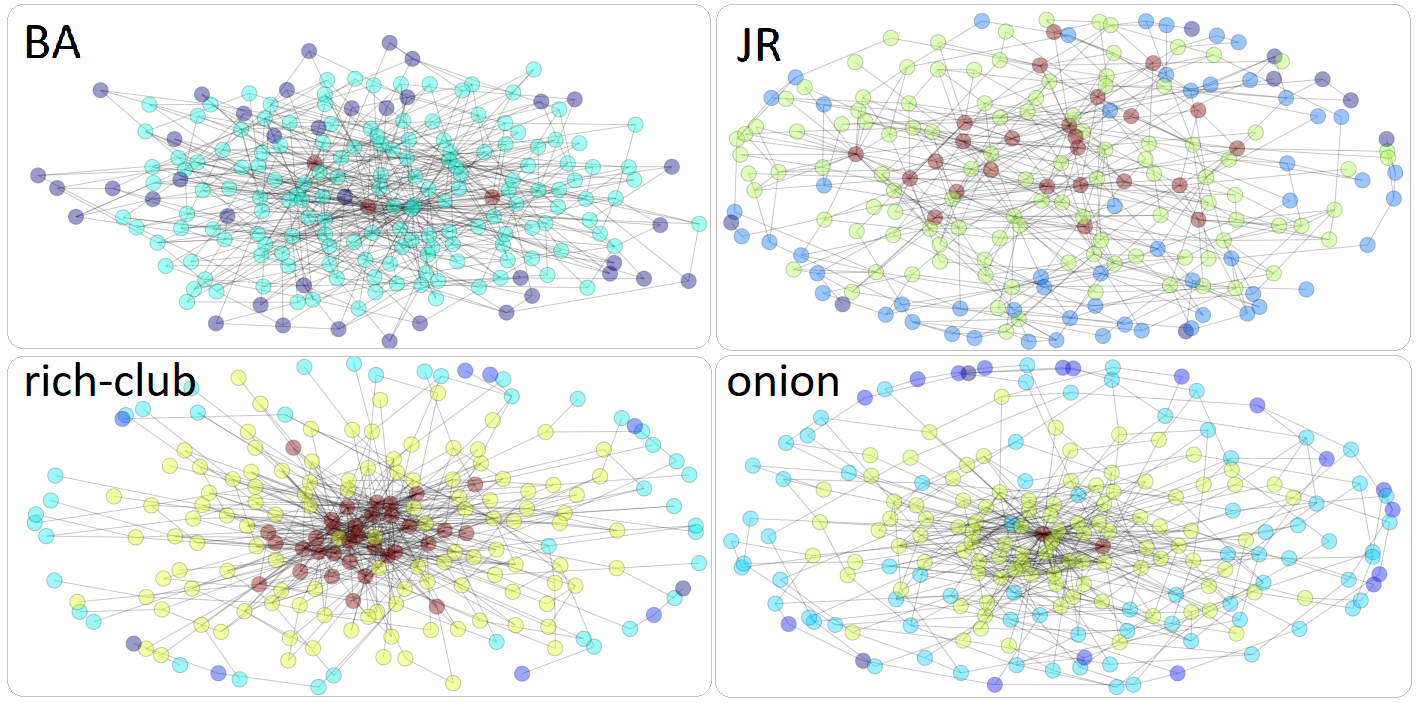
Table 2 summarizes key statistics of the models minding that they share the same parameter – average degree . Here we set to resemble values in empirical data sets11180 datasets on KONECT and SNAP have average degree between 2 and 10 http://konect.uni-koblenz.de/, http://snap.stanford.edu/, the network size 500 and the initial network being a cycle graph with length 10, as for BA model in [1]. For the JR model, a column is created for each value of . The rich-club and onion models have exceptionally high CP coefficient showing a clear core/periphery structure. Fig. 5 visually contrasts the four models clearly displaying the core in rich-club and onion, while for BA and JR the center is not clear.
| BA | JR0.25 | JR0.5 | JR1 | rich-club | onion | |
|---|---|---|---|---|---|---|
| clustering | 0.04 | 0.29 | 0.34 | 0.24 | 0.04 | 0.21 |
| max deg | 53.4 | 31.6 | 32.9 | 27.18 | 46.44 | 118 |
| center size | 120.5 | 33.0 | 47.1 | 19.18 | 27.16 | 3 |
| diameter | 5.6 | 8.3 | 7.84 | 6.54 | 9.46 | 7.4 |
| radius | 4 | 5 | 4.7 | 4.08 | 5.2 | 4.18 |
| cp-coef | -0.09 | 0.04 | 0.02 | -0.05 | 0.13 | 0.26 |
Experiment 2.
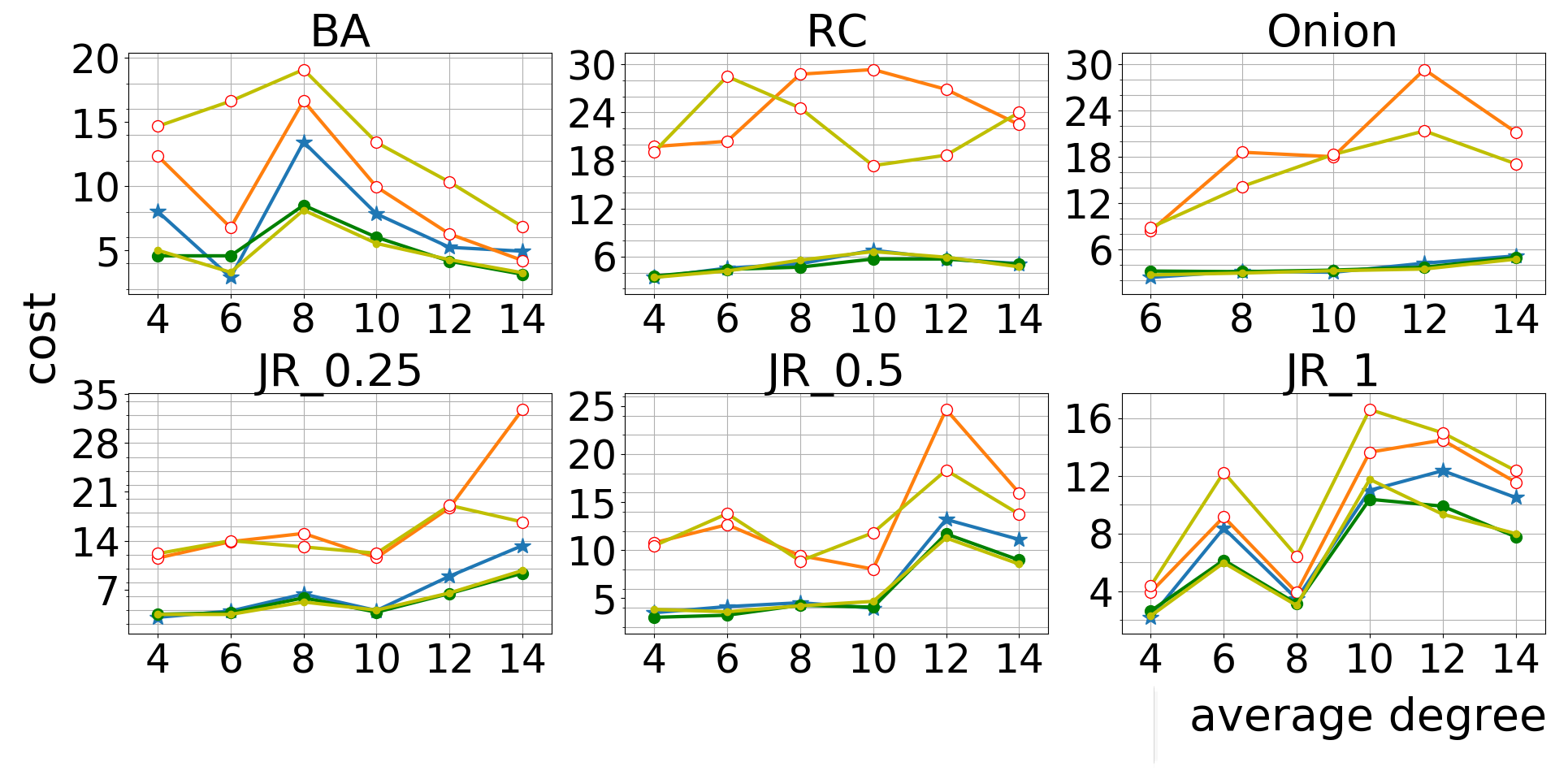
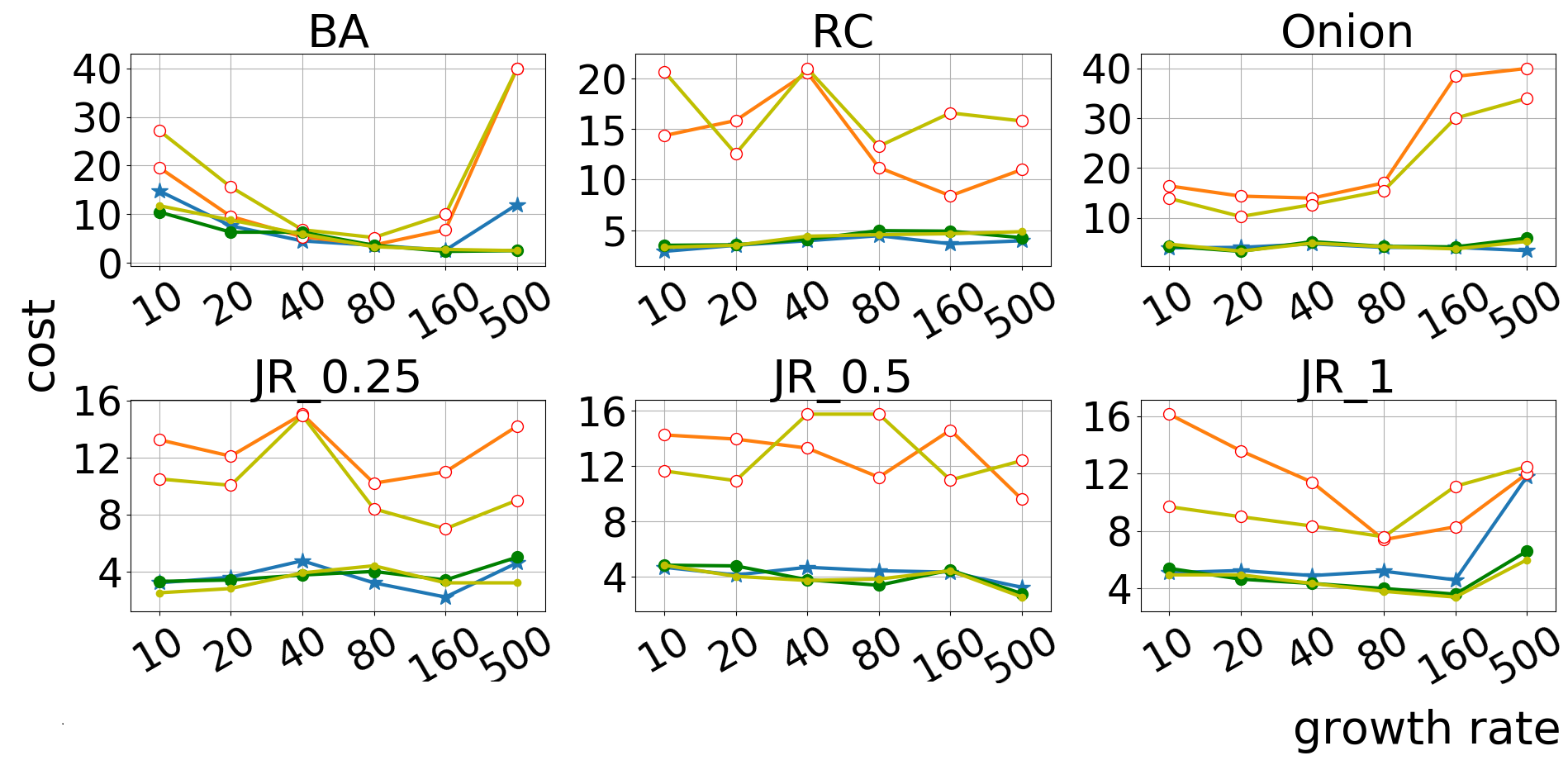
We run all tactics treating & as benchmarks over synthetic dynamic networks. IPs are simulated using the models above; the initial network is generated by the corresponding model and has size 500. There are several parameters which we may adjust. The first is the average degree which corresponds to the speed of adding edges to the network at each timestamp. The second is the growth rate of the network, which is the number of vertices that can be added in each timestamp. Firstly, we take and fix ; the costs of all tactics are plotted in Fig. 6. Then, we fix and adjust from 10 to 500; the costs are plotted in Fig. 7 (so that the resulting IP is -confined). All values in Fig. 6 and Fig. 7 are averaged among 100 trials.
We make several discussions: Apparent from the plots, , and MUF places into the center with much less costs compared to the benchmarks; The cost of these tactics is also very stable where the cost remains below 10 for every model even when or . Recall from Thm. 2 that when the network expands more rapidly, potentially no broker tactic would exist leading to an infinite cost; our experiment show that this would not happen for the four models of dynamic networks. The gap in cost between //MUF and / gets very wide (5 - 8 times) for models with a high CP-coefficient (rich-club, onion). This may be due to dense ties among core members resulting in them being excluded by /.
-
Tactics have relatively similar performance over BA and JR-1 networks; This may be due to the lack of a tight-knit core in these two models.
-
A faster growth rate (with a fixed ) would not affect the costs of tactics as the tactics exploit the central vertices which are relatively stable regardless of .
-
The vertices with high betweenness tend to locate around the center, so tactics with maximum betweenness have better performance on high CP-coefficient networks.
6 Conclusion and Future Work
We develop a structural investigation into the process where a newcomer integrates into a dynamic network through building ties. Our conclusions concern with conditions that warrant the existence of a broker tactic and simple cost-effective tactics over center/periphery networks. Five tactics are extensively compared on four real world datasets and four dynamic network models.
Modeling network dynamics has posed many challenges and we hope this work addresses some of them by providing a new angle and further insights. Many future work remain: (1) It is a natural question to explore dynamic models where ties are added as well as severed. (2) A distinction exists between the notions of network core and center [2]; A future question would be to investigate tactics that place the newcomer into the core, rather than just the network center. (3) Community structure is another prevalent meso-scale property and the same question could be targeted at dynamic community structure models. (4) Moving from the tactics of a single agent to a population of agents, one may formulate and investigate game-theoretical models of network formation based on the notions of social capital.
References
- [1] Albert-László Barabási and Réka Albert. Emergence of scaling in random networks. science, 286(5439):509–512, 1999.
- [2] Stephen Borgatti and Martin Everett. Models of core/periphery structures. social networks, 21(4):375–395, 2000.
- [3] Stephen Borgatti and Martin G Everett. A graph-theoretic perspective on centrality. social networks, 28(4):466–484, 2006.
- [4] Stephen Borgatti and Daniel Halgin. On network theory. Organization science, 22(5):1168–1181, 2011.
- [5] Stefan Bornholdt and Holger Ebel. World wide web scaling exponent from simon’s 1955 model. Phys Rev E, 64(3):035104, 2001.
- [6] Simina Brânzei and Kate Larson. Social distance games. In AAMAS-2011, pages 1281–1282. International Foundation for Autonomous Agents and Multiagent Systems, 2011.
- [7] Robert Christley, Pinchbeck, Bowers, Clancy, French, Bennett, and Turner. Infection in social networks: using network analysis to identify high-risk individuals. AJE, 162(10):1024–1031, 2005.
- [8] Peter Csermely, András London, Ling-Yun Wu, and Brian Uzzi. Structure and dynamics of core/periphery networks. Journal of Complex Networks, 1(2):93–123, 2013.
- [9] Daniel Fricke and Thomas Lux. Core–periphery structure in the overnight money market: evidence from the e-mid trading platform. COMPUT ECON, 45(3):359–395, 2015.
- [10] Ivan Galov, Aleksandr Lomov, and Dmitry Korzun. Design of semantic information broker for localized computing environments in the internet of things. In FRUCT-2015, pages 36–43. IEEE, 2015.
- [11] John Michael Harris, Jeffry Hirst, and Michael Mossinghoff. Combinatorics and graph theory, volume 2. Springer, 2008.
- [12] Petter Holme. Core-periphery organization of complex networks. Phys Rev E, 72(4):046111, 2005.
- [13] Jukka Honkola, Hannu Laine, Ronald Brown, and Olli Tyrkkö. Smart-m3 information sharing platform. In ISCC-2010, pages 1041–1046. IEEE, 2010.
- [14] Matthew Jackson. Social and economic networks. Princeton university press, 2010.
- [15] Matthew. Jackson and Stephen Nei. Networks of military alliances, wars, and international trade. PNAS, 112(50):15277–15284, 2015.
- [16] Matthew Jackson and Brian Rogers. Meeting strangers and friends of friends: How random are social networks? AER, 97(3):890–915, 2007.
- [17] Paul Krugman and Anthony Venables. Globalization and the inequality of nations. QJE, 110(4):857–880, 1995.
- [18] Srijan Kumar, Francesca Spezzano, Subrahmanian, and Christos Faloutsos. Edge weight prediction in weighted signed networks. In ICDM-2016, pages 221–230. IEEE, 2016.
- [19] Jure Leskovec, Jon Kleinberg, and Christos Faloutsos. Graph evolution: Densification and shrinking diameters. TKDD, 1(1):2, 2007.
- [20] Jiamou Liu and Anastasia Moskvina. Hierarchies, ties and power in organizational networks: model and analysis. Social Network Analysis and Mining, 6(1):106, 2016.
- [21] Anastasia Moskvina and Jiamou Liu. How to build your network? a structural analysis. In IJCAI-2016, pages 2597–2603. AAAI Press, 2016.
- [22] John Padgett and Christopher Ansell. Robust action and the rise of the medici, 1400-1434. AJS, 98(6):1259–1319, 1993.
- [23] Pietro Panzarasa, Tore Opsahl, and Kathleen Carley. Patterns and dynamics of users’ behavior and interaction: Network analysis of an online community. JAIST, 60(5):911–932, 2009.
- [24] Puck Rombach, Mason Porter, James Fowler, and Peter Mucha. Core-periphery structure in networks (revisited). SIAM Review, 59(3):619–646, 2017.
- [25] Brian Uzzi and Shannon Dunlap. How to build your network. Harvard business review, 83(12):53, 2005.
- [26] Stanley Wasserman and Katherine Faust. Social network analysis: Methods and applications, volume 8. Cambridge University Press, 1994.
- [27] Zhi-Xi Wu and Petter Holme. Onion structure and network robustness. Phys Rev E, 84(2):026106, 2011.
- [28] Bo Yan, Yang Chen, and Jiamou Liu. Dynamic relationship building: Exploitation versus exploration on a social network. In WISE-2017, pages 75–90. Springer, 2017.