Comparison analysis on two numerical methods for fractional diffusion problems based on rational approximations of $t^{\gamma},\ 0\leq t\leq 1$

Abstract.

We discuss, study, and compare experimentally three methods for solving the system of algebraic equations ${\mathbb{A}}^{\alpha}{\bf u}={\bf f}$, $0<\alpha<1$, where ${\mathbb{A}}$ is a symmetric and positive definite matrix obtained from finite difference or finite element approximations of second order elliptic problems in $\mathbb{R}^{d}$, $d=1,2,3$. The first method, introduced in [5], based on the best uniform rational approximation (BURA) $r_{\alpha}(t)$ of $t^{1-\alpha}$ for $0\leq t\leq 1$, is used to get the rational approximation of $t^{-\alpha}$ in the form $t^{-1}r_{\alpha}(t)$. Here we develop another method, denoted by R-BURA, that is based on the best rational approximation $r_{1-\alpha}(t)$ of $t^{\alpha}$ on the interval $[0,1]$ and approximates $t^{-\alpha}$ via $r^{-1}_{1-\alpha}(t)$. The third method, introduced and studied by Bonito and Pasciak in [2], is based on an exponentially convergent quadrature scheme for the Dundord-Taylor integral representation of the fractional powers of elliptic operators. All three methods reduce the solution of the system ${\mathbb{A}}^{\alpha}{\bf u}={\bf f}$ to solving a number of equations of the type $({\mathbb{A}}+c\mathbb{I}){\bf u}={\bf f}$, $c\geq 0$. Comprehensive numerical experiments on model problems with ${\mathbb{A}}$ obtained by approximation of elliptic equations in one and two spatial dimensions are used to compare the efficiency of these three algorithms depending on the fractional power $\alpha$. The presented results prove the concept of the new R-BURA method, which performs well for $\alpha$ close to $1$ in contrast to BURA, which performs well for $\alpha$ close to $0$. As a result, we show theoretically and experimentally, that they have mutually complementary advantages.

1. Introduction

1.1. Algebraic problems under consideration

Now let $\mathbb{R}^{N}$, $N$ positive integer, be an $N$-dimensional vector space with the standard $\ell_{2}$-inner product, ${\bf u}^{T}{\bf v}$, for any real vectors ${\bf u},{\bf v}\in\mathbb{R}^{N}$, and let ${\mathbb{A}}\in\mathbb{R}^{N\times N}$ be a symmetric and positive definite matrix with eigenvalues and eigenvectors $\{(\lambda_{i},{\bf\Psi}_{i})\}_{i=1}^{N}$. We assume that the eigenvectors are orthonormal, that is ${\bf\Psi}_{i}^{T}{\bf\Psi}_{j}=\delta_{ij}$, and $0<\lambda_{1}\leq\lambda_{2}\leq\dots\lambda_{N}$.

For $0<\alpha<1$ and given ${\bf f}\in\mathbb{R}^{N}$ we consider the following algebraic problem:

(1) $$\mbox{find }~{}~{}{\bf u}\in\mathbb{R}^{N}~{}~{}\mbox{such that }\quad{{\mathbb{A}}}^{\alpha}{\bf u}={\bf f}$$

where the fractional power ${\mathbb{A}}^{\alpha}$ is defined through eigenvalues and eigenvectors of ${\mathbb{A}}$

$${\mathbb{A}}^{\alpha}=\mathbb{W}{\mathbb{D}}^{\alpha}\mathbb{W}^{T},\ \ \mbox{ where }\ \ {\mathbb{A}}=\mathbb{W}{\mathbb{D}}\mathbb{W}^{T}.$$

Here $\mathbb{W},{\mathbb{D}}\in\mathbb{R}^{N\times N}$ are defined as $\mathbb{W}=[{\bf\Psi}_{1}^{T},{\bf\Psi}_{2}^{T},...,{\bf\Psi}_{N}^{T}]$ and ${\mathbb{D}}=diag(\lambda_{1},\dots,\lambda_{N})$. Then ${\mathbb{A}}^{-\alpha}=\mathbb{W}{\mathbb{D}}^{-\alpha}\mathbb{W}^{T}$ and the solution of ${\mathbb{A}}^{\alpha}{\bf u}={\bf f}$ can be expressed as

(2) $${{\bf u}}={\mathbb{A}}^{-\alpha}{\bf f}=\mathbb{W}{\mathbb{D}}^{-\alpha}\mathbb{W}^{T}{\bf f}.$$

For any $\beta\in\mathbb{R}$ we have $\|{\bf u}\|_{{\mathbb{A}}^{\beta+\alpha}}=\|{\bf f}\|_{{\mathbb{A}}^{\beta-\alpha}}$, where $\|{\bf u}\|^{2}_{{\mathbb{A}}^{\gamma}}={\bf u}^{T}{\mathbb{A}}^{\gamma}{\bf u},\ \gamma\in\mathbb{R}.$

1.2. Examples of SPD matrices under consideration

1.2.1. Example 1.

The first example of such a matrix is ${\mathbb{A}}\in\mathbb{R}^{N\times N}$, $N=n^{2}$, that has the following block stricture (here ${\mathbb{A}}_{i,i}\in\mathbb{R}^{n\times n}$, $i=1,\cdots,n$ and ${\mathbb{I}}_{n}$ is the identity matrix in $\mathbb{R}^{n}$)

(3) $${\mathbb{A}}=(n+1)^{2}\left[\begin{array}[]{ccccc}{\mathbb{A}}_{1,1}&-{\mathbb{I}}_{n}&&&\\ -{\mathbb{I}}_{n}&{\mathbb{A}}_{2,2}&-{\mathbb{I}}_{n}&&\\ \cdots&\cdots&\cdots&\cdots&\cdots\\ &-{\mathbb{I}}_{n}&{\mathbb{A}}_{i,i}&-{\mathbb{I}}_{n}&\\ \cdots&\cdots&\cdots&\cdots&\cdots\\ &&&-{\mathbb{I}}_{n}&{\mathbb{A}}_{n,n}\end{array}\right],\quad{\mathbb{A}}_{i,i}=\left[\begin{array}[]{cccc}4&-1&&\\ -1&4&-1&\\ \cdots&\cdots&\cdots&\cdots\\ &-1&4&-1\\ &&-1&4\end{array}\right].$$

This matrix is generated by the finite difference approximation of the following boundary value problem

(4) $$\begin{split}-\Delta u=f,\ \ x\in\Omega=(0,1)\times(0,1),\ \ u=0,\ \ x\in\partial\Omega\end{split}$$

on a uniform mesh with mesh-size $h=1/(n+1)$.

For a given ${\bf f}\in\mathbb{R}^{N}$ the algebraic problem

(5) $$\mbox{ find }{\bf u}\in\mathbb{R}^{N}\ \ \mbox{ that satisfies }\ \ {{\mathbb{A}}}^{\alpha}{\bf u}={\bf f}$$

is an approximation to the boundary value problem

(6) $$(-\Delta)^{\alpha}u=f,\ \ x\in\Omega=(0,1)\times(0,1),\ \ u=0,\ \ x\in\partial\Omega$$

with ${\bf f}$ being a projection of $f(x)$ onto the space of mesh functions.

We are not aware of rigorous analysis of the approximation properties of problem (5). However, this linear system approximates (4) due to its relation of the finite element approximation on a triangular mesh, discussed below.

1.2.2. Example 2.

We partition $\Omega=(0,1)\times(0,1)$ into squares of size $h=1/(n+1)$. Let ${\mathcal{T}}_{h}$ be obtained by subdividing each square into two triangles by connecting the upper left corner with the lower right corner. On this triangulation we introduce the space $V_{h}\subset H^{1}_{0}(\Omega)$ of continuous piece-wise linear function. The finite element approximation of (4) is: find $u_{h}\in V_{h}$ such that

(7) $$a(u_{h},v):=\int_{\Omega}\nabla u_{h}(x)\cdot\nabla v(x)dx=(f,v):=(\pi_{h}f,v)\ \ \forall v\in V_{h}.$$

Here $(\cdot,\cdot)$ is the standard $L_{2}$-inner product on $V_{h}$. We define the operator ${\mathrm{A}}:V_{h}\to V_{h}$ by $({\mathrm{A}}u,v)=(z,v)$ for all $v\in V_{h}$. Then ${\mathrm{A}}y=z\in V_{h}$ should have representation through the nodal basis $\psi_{k}$: $z=\sum c_{k}\psi_{k}$ and then the operator ${\mathrm{A}}$ is expressed through the global “stiffness” matrix $\{{\mathbb{A}}\}_{i,k}=a(\psi_{i},\psi_{k})$ and the global “mass” matrix ${\mathbb{M}}=\{(\psi_{i},\psi_{k})\}_{i,k}$ via the relation ${\mathrm{A}}={{\mathbb{M}}}^{-1}{{\mathbb{A}}}$.

The matrix ${{\mathbb{M}}}$ is not diagonal and has similar sparsity pattern as the the “stiffness” matrix ${{\mathbb{A}}}$. The algebraic problem

(8) $${\mathrm{A}}^{\alpha}u_{h}=\pi_{h}f$$

is stable and $u_{h}(x)=\sum_{i=1}^{N}u_{i}\psi_{i}(x),\ {\bf u}=\{u_{1},\cdots,u_{N}\}^{T}$ approximates the solution $u(x)$ of (6), see, [2].

In order to get the matrix ${\mathbb{A}}$, as need in (5), (instead of ${{\mathrm{A}}}$) we can apply the following approach. First, we introduce the “lumped” mass inner product in $V_{h}$, [15, pp.239–242]. Namely, for $z,v\in V_{h}$ we define

$$(z,v)_{h}=\frac{1}{3}\sum_{\tau\in{\mathcal{T}}_{h}}\sum_{i=1}^{3}|\tau|\ z(P_{i})v(P_{i}),\ \ \mbox{and lumped ``mass" matrix}\ \ {{\mathbb{M}}}=\{(\psi_{i},\psi_{k})_{h}\}_{i,k},$$

where $P_{1},P_{2},P_{3}$ are the vertexes of the triangle $\tau$ and $|\tau|$ is its area. Note that the lumped mass matrix ${{\mathbb{M}}}_{h}$ is diagonal! Moreover, since the mesh is square, all diagonal elements of ${{\mathbb{M}}}^{-1}_{h}$ are equal to $h^{-2}=(n+1)^{2}$ and ${{\mathrm{A}}}:V_{h}\to V_{h}$ is defined by

$$({{\mathrm{A}}}u_{h},v)_{h}=a(u_{h},v)\ \ \mbox{ gives }\ \ {\mathrm{A}}={{\mathbb{M}}}^{-1}{{\mathbb{A}}}.$$

Since on a uniform mesh $(\cdot,\cdot)_{h}$ is a good approximation of $(\cdot,\cdot)$ then one concludes that (5) approximates the problem (6).

1.2.3. Example 3.

Similar considerations could be also used in solving elliptic problem with non-constant coefficient in the reaction term generated by the weak form

(9) $$A(u_{h},v):=a(u_{h},v)+(qu_{h},v)_{h}=(f,v)\ \ \forall v\in V_{h},$$

with $q=q(x)\geq 0$. The bilinear form is symmetric and coercive on $V_{h}$ and the corresponding algebraic problem will have the same properties as the one involving Laplace operator. Then the matrix of the corresponding linear system is the sum ${\mathbb{A}}+{\mathbb{D}},$ where ${\mathbb{D}}$ is a diagonal matrix in $\mathbb{R}^{N}$ with entries the values of $q(x)$ at the mesh points.

Remark 1.1.

One can generate matrices with similar structure while solving elliptic problems with Neumann or Robin boundary conditions.

1.3. The concept of the best uniform rational approximation (BURA)

We shall use the following notation for a class of rational functions:

$$\mathcal{R}(k,m)=\{r(t):~{}r(t)=P_{k}(t)/Q_{m}(t),\ \ \mbox{where}\ P_{k}\in{\mathcal{P}}_{k},\ \mbox{and }\ Q_{m}\in{\mathcal{P}}_{m},\ \mbox{monic}\}$$

with ${\mathcal{P}}_{j}$ set of algebraic polynomials of degree $j$. The best uniform approximation $r_{\alpha}(t)\in\mathcal{R}(k,m)$ of $t^{1-\alpha}$ on $[0,1]$ (called further $(k,m)$-BURA), and its approximation error $E_{\alpha,k,m}$ are defined as follows:

$$r_{\alpha}(t):=\mathop{\rm argmin}_{r\in\mathcal{R}(k,m)}\left\|t^{1-\alpha}-r(t)\right\|_{L^{\infty}(0,1)},\ \ \varepsilon(t)=r_{1-\alpha}(t)-t^{\alpha},\ \ E_{\alpha,k,m}:=\|\varepsilon(t)\|_{L^{\infty}(0,1)}.$$

For $k=m$ the existence and uniqueness of $r_{\alpha}(t)$ has been established long time ago [11, Chapters 9.1 and 9.2]. Moreover, it is known that both the numerator and the denominator of the minimizer are of exact degree $k$ and the error function $\varepsilon(t)$ possesses $2k+2$ extreme points in $[0,1]$, including the endpoints of the interval.

1.4. Methods for solving equations involving functions of matrices

The formula (2) could be used in practical computations if the eigenvectors and eigenvalues are explicitly known and Fast Fourier Transform is applicable to perform the matrix vector multiplication with $\mathbb{W}$, thus leading to almost optimal computational complexity, $O(N\log N)$. However, this approach is limited to separable problems with constant coefficients in simple domains and boundary conditions.

This work is related also to the more difficult problem of stable computations of the matrix square root and other functions of matrices, see, e.g. the earlier papers [3, 7, 10], as well as, [4] for some more recent related results. However, in this paper we do not deal with evaluation of ${\mathbb{A}}^{\alpha}$, instead we discuss efficient methods for solving the algebraic system ${\mathbb{A}}^{\alpha}{\bf u}={\bf f}$, where ${\mathbb{A}}$ is an SPD matrix generated by approximation of second order elliptic operators.

Our research is also connected with the work done in [8, 9], where numerical approximation of a fractional-in-space diffusion equation is considered. In [9], the proposed solver relies on Lanczos method. First, the adaptively preconditioned thick restart Lanczos procedure is applied to a system with ${\mathbb{A}}$. The gathered spectral information is then used to solve the system with ${\mathbb{A}}^{\alpha}$. In [3] an extended Krylov subspace method is proposed, originating by actions of the SPD matrix and its inverse. It is shown that for the same approximation quality, the variant of the extended subspaces requires about the square root of the dimension of the standard Krylov subspaces using only positive or negative matrix powers. A drawback of this method is the memory required to store the full dense matrix $\mathbb{W}$, and the substantial deterioration of the convergence rate for ill-conditioned matrices. The advantage of the approach discussed in this paper is the robustness and almost optimal computational complexity.

1.5. Our contributions

We investigate two approaches for approximate solving of ${\mathbb{A}}^{-\alpha}\bf f$ that are based on the best uniform rational approximation (BURA) $r(t)$ of $t^{\gamma}$, $\gamma>0$, on $[0,1]$. One subclass of such approximations is expressed through diagonal Walsh table $P_{k}(t)/Q_{k}(t)$, i.e. $r\in{\mathcal{R}}(k,k)$, see, e.g. [14, 16]. Another subclass is the upper diagonal $P_{k+1}(t)/Q_{k}(t)$, i.e., $r\in{\mathcal{R}}(k+1,k)$. The first analyzed method is introduced in [5], where the BURA $r_{\alpha}(t)$ of $t^{1-\alpha}$, $0<t\leq 1$, introduces a rational approximation of $t^{-\alpha}$ in the form $t^{-1}r_{\alpha}(t)$. Here we develop a new method, denoted by R-BURA, where the best uniform rational approximation $r_{1-\alpha}(t)$ of $t^{\alpha}$ is used to approximate $t^{-\alpha}$ by $1/r_{1-\alpha}(t)$. Both methods reduce solving (1) to a number of equations $({\mathbb{A}}+c{\mathbb{I}}){\bf u}={\bf F}$, $c\geq 0$.

Our comparative analysis includes also the method proposed in [2] that is based on approximation of the integral representation of the solution of (6). Then exponentially convergent quadrature formulae are applied to evaluate numerically the related integrals. In fact, this Q-method leads also to a rational approximation as well. The problem with checkerboard right hand side, introduced in [2], is used in the numerical tests of our comparative analysis.

The rest of the paper is organized as follows. In Section 2 we introduce the basic properties of the studied solution methods and algorithms. The analysis includes error estimates of the BURA, [5], the new R-BURA, and Q-method of Bonito and Pasciak, [2]. Section 3 contains numerical tests for fractional Laplace problems. In the case of BURA and R-BURA solvers, the impact of scaling is analyzed and experimentally confirmed. Among others, the numerical results complete the proof of concept of the new R-BURA approach, illustrating its advantages in the case of larger $\alpha\in(1/2,1)$.

2. Description of the numerical methods

2.1. The BURA method

In this paper we consider two BURA subclasses $(k,k)$ and $(k+1,k)$, introduced in Section 1.5. Let ${\Lambda}:=\|{\mathbb{A}}\|_{\infty}=\max_{1\leq i\leq N}\sum_{j=1}^{N}|a_{ij}|$. Following [5], we obtain the rescaled SPD matrix ${\mathcal{A}}:={\Lambda}^{-1}{\mathbb{A}}$ with spectrum in $(0,1]$. Then the original problem ${\mathbb{A}}^{\alpha}{\bf u}={\bf f}$ can be rewritten as ${\mathcal{A}}^{\alpha}{\bf u}={\Lambda}^{-\alpha}{\bf f}$. Note that the eigenvalues of ${\mathcal{A}}$ are $\mu_{i}:={\Lambda}^{-1}\lambda_{i}$, $0<\mu_{i}\leq 1$, $i=1,\cdots,N$.

Let $r_{\alpha}(t)$ be the BURA of $t^{1-\alpha}$ in ${\mathcal{R}}(k,k)$ or ${\mathcal{R}}(k+1,k)$. Then

(10) $${\bf u}_{r}:={\Lambda}^{-\alpha}{\mathcal{A}}^{-1}r_{\alpha}({\mathcal{A}}){\bf f},$$

are called $(k,k)$-BURA and $(k+1,k)$-BURA approximation of ${\bf u}$, respectively.

Using the spectral decomposition of ${\mathbb{A}}$, we can derive the following estimation of the BURA error:

(11) $$\frac{\|{\bf u}_{r}-{\bf u}\|_{2}}{\|{\bf f}\|_{2}}={\Lambda}^{-\alpha}\max_{\mu_{i}}\frac{\left|r_{\alpha}(\mu_{i})-\mu_{i}^{1-\alpha}\right|}{\mu_{i}}\leq\frac{{\Lambda}^{1-\alpha}E_{\alpha,k,m}}{\lambda_{1}}.$$

Then using [13, Theorem 1] (about the behavior of $E_{\alpha,k.k}$ as $k\to\infty$) we get the following property of the $(k,k)$-BURA:

(12) $$\lim_{k\to\infty}e^{2\pi\sqrt{(1-\alpha)k}}\|{\bf u}_{r}-{\bf u}\|_{2}=\frac{4^{2-\alpha}{\Lambda}^{1-\alpha}}{\lambda_{1}}\sin(\pi\alpha)\|{\bf f}\|_{2}.$$

Since $E_{\alpha,k,k}\geq E_{\alpha,k+1,k}\geq E_{\alpha,k+1,k+1}$ by definition, (12) is valid for $(k+1,k)$-BURA, as well.

We restricted our experiments to $(k,k)$-BURA method. The implementation uses the decomposition of the rational function $t^{-1}r_{\alpha}(t)$ into sum of partial fractions so that

$${\bf u}_{r}=\sum_{j=0}^{k}c_{j}({\mathcal{A}}-d_{j}{{\mathbb{I}}})^{-1}{\bf f}={\Lambda}\sum_{j=0}^{k}c_{j}({\mathbb{A}}-{\Lambda}d_{j}{{\mathbb{I}}})^{-1}{\bf f}.$$

Here $0=d_{0}>d_{1}\dots>d_{k}$ are the poles of $r_{\alpha}(t)$ plus the additional pole at zero, and $c_{j}>0$ for every $j$ (see [12] for more details). Obviously, the approximation ${\bf u}_{r}$ is obtained by solving $k+1$ linear systems with nonnegative diagonal shifts of ${\mathbb{A}}$.

2.2. The R-BURA method

In this approach, we approximate $t^{-\alpha}$ by $r^{-1}_{1-\alpha}(t)$ where $r_{1-\alpha}(t)$ is the best rational approximation of $t^{\alpha}$ in ${\mathcal{R}}(k,k)$ or ${\mathcal{R}}(k+1,k)$. Then

(13) $${\bf u}_{r}:={\Lambda}^{-\alpha}r^{-1}_{1-\alpha}({\mathcal{A}}){\bf f}$$

are called $(k,k)$-R-BURA and $(k+1,k)$-R-BURA approximation of ${\bf u}$, respectively.

For the analysis of the BURA-method we shall need the following properties of $r_{\alpha}(t)$:

Lemma 2.1.

Let $\alpha\in(0,1)$ and $k$ be a positive integer. Then the best rational approximation (BURA) $r_{\alpha}(t)\in\mathcal{R}({k,k})$ of $t^{1-\alpha}$ in $[0,1]$ has the following properties:

• $r_{\alpha}(t)$ is strictly monotonically increasing concave function when $t\in[0,1]$;

• $r_{\alpha}(0)=E_{\alpha,k,k}$.

Proof.

The second part follows directly from [12, Lemma 2.1], where it is shown that $\eta_{1}=0$ is an extreme point for $t^{1-\alpha}-r_{\alpha}(t)$ with negative value. The same lemma states that all the $k$ zeros and $k$ poles (denoted by $d_{j}$) of $r_{\alpha}$ are real, pairwise different, non-positive, and interlacing. Then for the decomposition of $r_{\alpha}(t)$ into partial fractions

$$r_{\alpha}(t)=b^{\ast}_{0}+\sum_{j=1}^{k}\frac{c^{\ast}_{j}}{t-d_{j}}$$

we have $c_{j}^{\ast},d_{j}<0$, $j=1,\cdots,m$, for more details, see, e.g. [6, Theorem 1]. Hence,

$$\begin{split}r^{\prime}_{\alpha}(t)=\sum_{j=1}^{k}\frac{-c^{\ast}_{j}}{(t-d_{j})^{2}}>0,\qquad r^{\prime\prime}_{\alpha}(t)=\sum_{j=1}^{k}\frac{2c^{\ast}_{j}}{(t-d_{j})^{3}}<0,\qquad\forall t\in[0,1].\end{split}$$

The proof is completed. ∎

Applying Lemma 2.1, the $(k,k)$-R-BURA approximation error is estimated analogously to the BURA error:

$$\frac{\|{\bf u}_{r}-{\bf u}\|_{2}}{\|{\bf f}\|_{2}}\leq{\Lambda}^{-\alpha}\max_{\mu_{i}}\frac{\left|r_{1-\alpha}(\mu_{i})-\mu_{i}^{\alpha}\right|}{\mu^{\alpha}_{i}r_{1-\alpha}(\mu_{i})}\leq\frac{{\Lambda}^{-\alpha}E_{1-\alpha,k,k}}{\mu^{\alpha}_{1}r_{1-\alpha}(\mu_{1})}\leq\frac{E_{1-\alpha,k,k}}{\lambda^{\alpha}_{1}r_{1-\alpha}(\mu_{1})}.$$

Note that, $r_{1-\alpha}(t)$ has no zeros inside the interval $t\in[0,1]$, therefore the denominator is strictly positive and the error bound is well-defined. On the other hand, $r_{1-\alpha}(0)=E_{1-\alpha,k,k}$ when $h\to 0$ then $\mu_{1}\to 0$ and the error deteriorates. The error function $\varepsilon(t)=r_{1-\alpha}(t)-t^{\alpha}$ has $2k+1$ roots $\{\xi_{i}\}_{1}^{2k+1}$ in $(0,1)$, due to the $2k+2$ extreme points, including $\{0,1\}$, see, e.g., [12]. Since $\varepsilon(0)=E_{1-\alpha,k,k}>0$, we have

(14) $$r_{1-\alpha}(t)\geq t^{\alpha},\qquad\forall t\in[0,\xi_{1}]\cup\bigcup\limits_{i=1}^{k}[\xi_{2i},\xi_{2i+1}].$$

Therefore, whenever $\mu_{1}$ is a priori estimated (enough to have a good lower bound for $\lambda_{1}$), we can choose a proper $k$, such that

(15) $$\frac{\|{\bf u}_{r}-{\bf u}\|_{2}}{\|{\bf f}\|_{2}}\leq\frac{E_{1-\alpha,k,k}}{\lambda^{\alpha}_{1}\mu^{\alpha}_{1}}=\frac{{\Lambda}^{\alpha}E_{1-\alpha,k,k}}{\lambda^{2\alpha}_{1}},\qquad\mu_{1}\in\bigcup\limits_{i=1}^{k}[\xi_{2i},\xi_{2i+1}].$$

The case $\mu_{1}\in[0,\xi_{1}]$ is more subtle and needs special care. Using $r_{1-\alpha}(t)=t^{\alpha}+\varepsilon(t)$, with $0<\varepsilon(t)\leq E_{1-\alpha,k,k}$, together with the fact that the function $g(\varepsilon):=\varepsilon/(\mu^{\alpha}_{1}+\varepsilon)$ is monotonically increasing for $\varepsilon\geq 0$ we obtain

$$\frac{\left|r_{1-\alpha}(\mu_{1})-\mu_{1}^{\alpha}\right|}{\mu^{\alpha}_{1}r_{1-\alpha}(\mu_{1})}\leq\frac{E_{1-\alpha,k,k}}{\mu^{\alpha}_{1}(\mu^{\alpha}_{1}+E_{1-\alpha,k,k})}\leq\frac{E_{1-\alpha,k,k}}{\mu^{\alpha}_{1}E_{1-\alpha,k,k}}.$$

For every $\mu_{i}>\xi_{1}$ we have

$$\frac{\left|r_{1-\alpha}(\mu_{i})-\mu_{i}^{\alpha}\right|}{\mu^{\alpha}_{i}r_{1-\alpha}(\mu_{i})}\leq\frac{E_{1-\alpha,k,k}}{\mu^{\alpha}_{i}r_{1-\alpha}(\xi_{1})}\leq\frac{E_{1-\alpha,k,k}}{\mu^{\alpha}_{1}\xi^{\alpha}_{1}}.$$

Therefore, since $\xi^{\alpha}_{1}=r_{1-\alpha}(\xi_{1})>r_{1-\alpha}(0)=E_{1-\alpha,k,k}$,

(16) $$\frac{\|{\bf u}_{r}-{\bf u}\|_{2}}{\|{\bf f}\|_{2}}\leq\frac{E_{1-\alpha,k,k}}{\lambda^{\alpha}_{1}\max(\xi^{\alpha}_{1},E_{1-\alpha,k,k})}=\lambda^{-\alpha}_{1},\qquad\forall\mu_{1}\in[0,\xi_{1}].$$

Typically $\lambda_{1}=\mathrm{O}(1)$ for all $h$ and $\mu_{1}\to 0$ as $h\to 0$, thus unlike the BURA case (11) the $(k,k)$-R-BURA relative error is uniformly bounded when $k$ is fixed and $h\to 0$.

The asymptotic behavior of the relative error (15) is derived analogously to (12):

(17) $$\lim_{k\to\infty}e^{2\pi\sqrt{\alpha k}}\|{\bf u}_{r}-{\bf u}\|_{2}=\frac{4^{2-\alpha}{\Lambda}^{\alpha}}{\lambda^{2\alpha}_{1}}\sin(\pi\alpha)\|{\bf f}\|_{2}.$$

In our experiments, we work with $r_{1-\alpha}$ in $\mathcal{R}(k+1,k)$ and $\mathcal{R}(k+1,k+1)$. Similar to BURA-method, the numerical computation of ${\bf u}_{r}$ involves solving of $k+1$ independent linear systems with nonnegative diagonal shifts of ${\mathbb{A}}$.

2.3. Q-method

The solver, proposed by Bonito and Pasciak in [2], incorporates an exponentially convergent quadrature scheme for the approximate computation of an integral solution representation, i.e., uses the rational function

$$Q_{\alpha}(t):=\frac{2k^{\prime}\sin(\pi\alpha)}{\pi}\sum_{\ell=-m}^{M}\frac{e^{2(\alpha-1)\ell k^{\prime}}}{t+e^{-2\ell k^{\prime}}},\qquad t\in(0,\infty),$$

where $m=\lceil(1-\alpha)k\rceil$, $M=\lceil\alpha k\rceil$, $k^{\prime}=\pi/(2\sqrt{\alpha(1-\alpha)k})$. Since

$$\lceil(1-\alpha)k\rceil+\lceil\alpha k\rceil=\left\{\begin{array}[]{lcl}k+1,&&\alpha k\notin\mathbb{Z}\\ k,&&\alpha k\in\mathbb{Z}\end{array}\right.$$

$Q_{\alpha}$ is either a $(k+1,k+1)$ or a $(k+2,k+2)$ rational function. The approximant of ${\bf u}_{h}$ has the form

(18) $${\bf u}_{Q}:=\frac{2k^{\prime}\sin(\pi\alpha)}{\pi}\sum_{\ell=-m}^{M}e^{2(\alpha-1)\ell k^{\prime}}\left({\mathbb{A}}+e^{-2\ell k^{\prime}}{\mathbb{I}}\right)^{-1}{\bf f}.$$

The parameter $k^{\prime}>0$ controls the accuracy of ${\bf u}_{Q}$ and the number of linear systems to be solved. For example, $k^{\prime}=1/3$ gives rise to 120 systems for $\alpha=\{0.25,0.75\}$ and $91$ systems for $\alpha=0.5$ guaranteeing $\|{\bf u}_{Q}-{\bf u}\|_{2}\approx 10^{-7}\|{\bf f}\|_{2}$. We have

(19) $$\frac{\|{\bf u}_{Q}-{\bf u}\|_{2}}{\|{\bf f}\|_{2}}\leq\max_{\lambda_{i}}\left|Q_{\alpha}(\lambda_{i})-\lambda_{i}^{-\alpha}\right|\approx\left|Q_{\alpha}(\lambda_{1})-\lambda^{-\alpha}_{1}\right|.$$

Finally, the error analysis, developed in [2] states

(20) $$\lim_{k\to\infty}e^{\pi\sqrt{\alpha(1-\alpha)k}}\|{\bf u}_{Q}-{\bf u}\|_{2}=\frac{2\sin(\pi\alpha)}{\pi}\left(\frac{1}{\alpha}+\frac{1}{(1-\alpha)\lambda_{1}}\right)\|{\bf f}\|_{2}.$$

Remark 2.2.

Varying the quadrature formulae, a family of related methods can be obtained. For example, Gauss-Jacobi quadrature rule is used to approximate the integral representation of the solution in [1].

2.4. Comparison of the three solvers

Comparing (12) with (20) we observe exponential decay of both errors with respect to the number of linear systems to be solved. The exponential order of the BURA estimate is at least twice higher than the one for the quadrature rule, but there is a multiplicative factor ${\Lambda}^{1-\alpha}$ in (12), which depends on the mesh size $h$ and ${\Lambda}\to\infty$ as $h\to 0$. This implies trade-off between numerical accuracy and computational efficiency for the BURA method. The choice of $k$ for $r_{\alpha}\in\mathcal{R}(k,k)$ should be synchronized with $h$, while the size of $h$ does not affect the choice of $k$ for $Q_{\alpha}$. Another difference between the two approaches is that the error bound in (12) is unbalanced and can be reached only for ${\bf f}={\bf\Psi}_{1}$ and only if ${\Lambda}^{-1}\lambda_{1}$ is an extreme point for $r_{\alpha}$ (see (11)), while the error bound in (20) is balanced. Hence, the BURA error heavily depends on the decomposition of the right-hand-side ${\bf f}$ along $\{{\bf\Psi}_{i}\}$ and possesses a wide range of values, while the quadrature error is independent on ${\bf f}$.

The errors in (11) and (15) are bounded by the expressions ${\Lambda}^{1-\alpha}E_{\alpha,k,k}/\lambda_{1}$ and ${\Lambda}^{\alpha}E_{1-\alpha,k,k}/\lambda^{2\alpha}_{1}$. Since $E_{\alpha,k,k}$ is monotonically increasing function with respect to $\alpha$ and ${\Lambda},\lambda_{1}>1$, for $\alpha>0.5$ the R-BURA method provides better theoretical error bounds, while for $\alpha<0.5$ so does the BURA one. In the case $\alpha=0.5$ the two approaches behave similarly. The drawback for the R-BURA method is the additional condition on $k$ and $h$, namely $\mu_{1}\in\bigcup\limits_{i=1}^{k}[\xi_{2i},\xi_{2i+1}]$. On the other hand, if we can guarantee this, then the R-BURA method has some advantage, as we solve one linear system less ($k+1$ for BURA vs $k$ for R-BURA, when using the same $(k,k)$ function $r_{0.5}(t)$). Below we provide an experimental comparison of these approaches for various $h$ and $k=\{7,8,9\}$.

3. Numerical tests: comparative analysis and proof of concept

We consider the fractional Laplace problem with homogeneous boundary conditions (6) in both 1-D and 2-D. In 1-D we use the well-known eigenvectors and eigenvalues of the corresponding SPD matrix for experimental validation of the theoretical error analysis. In 2-D we investigate the relation between numerical accuracy and computational efficiency of the considered three solvers.

3.1. Algorithm for computing BURA

Following [5] we consider $\alpha=\{0.25,0.5,0.75\}$ and investigate methods with similar computational efficiency. The rational functions $r_{\alpha}(t)$ are computed using the modified Remez algorithm, described in [5, Section 3.2]. In the case $\alpha=0.25$ we compare $(k,k)$-BURA with the $k$-Q-method, $k=9$. The corresponding numerical solvers incorporate $10$, respectively $11$ linear systems with positive diagonal shifts of ${\mathbb{A}}$. In the cases $\alpha=\{0.5,0.75\}$ we compare $(k,k)$-BURA, $(k+1,k)$-R-BURA, $(k+1,k+1)$-R-BURA, and $k$-Q-method for $k=7$. This gives rise to $k+1$ linear systems with positive diagonal shifts of ${\mathcal{A}}$ for the first two methods and $k+2$ linear systems with positive diagonal shifts for the last method.

Table 1. Errors $E_{\alpha,k,m}$ of $r_{\alpha}(t)$ for $t\in[0,1]$, used in the analysis of BURA and R-BURA numerical methods.

$\alpha$	$E_{\alpha,5,5}$	$E_{\alpha,6,6}$	$E_{\alpha,7,7}$	$E_{\alpha,8,7}$	$E_{\alpha,8,8}$	$E_{\alpha,9,8}$	$E_{\alpha,9,9}$	$E_{\alpha,10,9}$
0.25	2.8676e-5	9.2522e-6	3.2566e-6	1.9500e-6	1.2288e-6	7.5972e-7	4.9096e-7	3.1128e-7
0.50	2.6896e-4	1.0747e-4	4.6037e-5	3.0789e-5	2.0852e-5	$\ast$	$\ast$	$\ast$
0.75	2.7348e-3	1.4312e-3	7.8269e-4	$\ast$	$\ast$	$\ast$	$\ast$	$\ast$

The maximal approximation errors of the involved BURA functions are summarized in Table 1. We use $\ast$ to indicate errors that cannot be computed when the Quadruple-precision floating-point format is applied for the arithmetics. The first four zeros of the associated functions $\varepsilon(t)=r_{1-\alpha}(t)-t^{\alpha}$ are presented in Table 2. Note that they are needed only in the analysis of R-BURA setting, thus we exclude $\alpha=0.25$ where R-BURA behaves worse than BURA.

Table 2. First four roots of $\varepsilon(t)$ for $r_{1-\alpha}\in\mathcal{R}(k,m)$.

	First four zeros $\xi_{1},\xi_{2},\xi_{3},\xi_{4}$ of $\varepsilon(t)=r_{1-\alpha}(t)-t^{\alpha}$
$(k,m)$	$\alpha=0.50$				$\alpha=0.75$
	$\xi_{1}$	$\xi_{2}$	$\xi_{3}$	$\xi_{4}$	$\xi_{1}$	$\xi_{2}$	$\xi_{3}$	$\xi_{4}$
$(5,5)$	1.030e-7	6.732e-6	6.592e-5	4.352e-4	2.185e-6	7.269e-5	5.004e-4	2.353e-3
$(6,6)$	1.650e-8	1.076e-6	1.053e-5	6.950e-5	4.836e-7	1.609e-5	1.108e-4	5.216e-4
$(7,7)$	3.100e-9	1.981e-7	1.932e-6	1.275e-5	1.202e-7	3.999e-6	2.754e-5	1.297e-4
$(8,7)$	1.400e-9	8.840e-8	8.644e-7	5.705e-6	6.070e-8	2.019e-6	1.390e-5	6.544e-5
$(8,8)$	7.00e-10	4.070e-8	3.967e-7	2.617e-6	3.280e-8	1.091e-6	7.509e-6	3.536e-5

3.2. Numerical results for 1-D fractional Laplace problem

For this problem we have $\lambda_{1}=(4/h^{2})\sin^{2}(\pi h/2)$, ${\Lambda}=4/h^{2}$, and $\mu_{1}=\sin^{2}(\pi h/2)$. The numerical results are given on Figures 1 – 2.

First, we solve the system ${\mathbb{A}}^{\alpha}{\bf u}={\bf\Psi}_{1}$. The theoretical errors of the three methods, given by ${\Lambda}^{-\alpha}|\mu^{-1}_{1}r_{\alpha}(\mu_{1})-\mu^{-\alpha}_{1}|$ of BURA, ${\Lambda}^{-\alpha}|r_{1-\alpha}(\mu_{1})-\mu_{1}^{\alpha}|/(\mu^{\alpha}_{1}r_{1-\alpha}(\mu_{1}))$ of R-BURA, and $|Q_{\alpha}(\lambda_{1})-\lambda^{-\alpha}_{1}|$ of the Q-method, are presented as function of $h\in[10^{-7},10^{-2}]$ on Figure 1. The numerical results in each graph are obtained by comparable computational complexity (expressed through the number of systems solved).

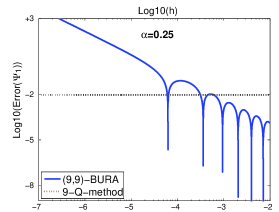
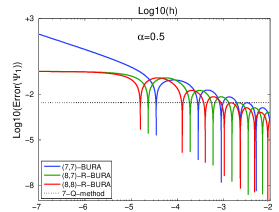
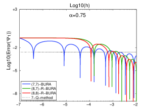
Figure 1. Comparison of the theoretical error bounds $\|{\bf u}_{r}-{\bf u}\|_{2}/\|{\bf f}\|_{2}$, ${\bf f}={\bf\Psi}_{1}$, of the three solvers with respect to $h$ for the 1-D fractional Laplacian.

The oscillating behavior of the BURA-related error is due to the placement of $\mu_{1}$ with respect to the extreme points of $\varepsilon(t)$. When $\alpha=0.75$, $k=8$ (right plot) and $h<10^{-4}$ we observe the constant asymptotic behavior of the R-BURA errors towards $\pi^{-2\alpha}$ as $h\to 0$. Similar observation is made for $\alpha=0.5$ and $h<2\cdot 10^{-5}$. Since $\mu_{1}\approx\pi^{2}h^{2}/4$, we have that $\mu_{1}\approx 2.5\cdot 10^{-8}$ for $\alpha=0.75$ and $h=10^{-4}$, which, as seen from Table 2, is close to the first zero $\xi_{1}$ of $\varepsilon(t)$ for the corresponding $(8,7)-$ and $(8,8)-$ approximations $r_{0.25}(t)$. This asymptotic behavior perfectly agrees with the error estimate (16). The same analysis can be made for $\alpha=0.5$ and $h=2\cdot 10^{-5}$, where $\mu_{1}\approx 5\cdot 10^{-10}$. The Q-method errors are independent of $h$. We observe that for $\alpha=0.5$ the BURA and R-BURA solvers have comparable accuracy over the whole interval $(0,1]$. For $\alpha=0.75$ and $h\in[10^{-4},10^{-3}]$, we observe that both $(8,7)-$ and $(8,8)$-R-BURA functions give worse relative errors than the $(7,7)$-BURA function, since $\mu_{1}\in[\xi_{1},\xi_{2}]$ (see Table 2).

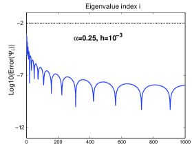
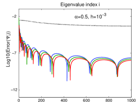
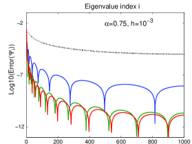
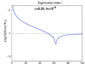
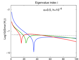
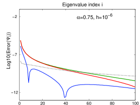
Figure 2. Spectral decomposition of the error for the 1-D fractional Laplace problem with $h=10^{-3}$ (top) and $h=10^{-6}$ (bottom). Colors are with respect to the legend of Fig. 1. Top: for each $i$ we plot the corresponding errors $\|{\bf u}_{r}-{\bf u}_{Q}\|_{2}/\|{\bf f}\|_{2}$ for ${\bf f}={\bf\Psi}_{i}$. The bottom plots present the corresponding errors for the first $100$ eigenvectors, i.e., for $\{{\bf\Psi}_{i}\}_{1}^{100}$ .

The second set of experiments deals with the error over the whole spectrum of ${\mathbb{A}}$ and is presented on Figure 2. For $h=10^{-3}$ and $h=10^{-6}$ we compute ${\Lambda}^{-\alpha}|\mu^{-1}_{i}r_{\alpha}(\mu_{i})-\mu^{-\alpha}_{i}|$, ${\Lambda}^{-\alpha}|r_{1-\alpha}(\mu_{i})-\mu_{i}^{\alpha}|/(\mu^{\alpha}_{i}r_{1-\alpha}(\mu_{i}))$, and $|Q_{\alpha}(\lambda_{i})-\lambda^{-\alpha}_{i}|$ for all $i$, which is equivalent to letting the right-hand-side in (5) run over the eigenvectors of ${\mathbb{A}}$ (${\bf f}={\bf\Psi}_{i}$). The plots on the first row illustrate the complete spectral decomposition of the error for $h=10^{-3}$. For $h=10^{-6}$ we show the spectral error over the first $1\%$ of the eigen-modes on the second row. The unbalanced behavior of the BURA-related errors in contrast to the balanced behavior of the errors of the Q-method is clearly observed. High-frequency modes are practically perfectly reconstructed by the R-BURA methods, while the low-frequency ones lead to larger errors. When $h=10^{-3}$ and $k$ is chosen accordingly, all BURA-related errors are smaller than the corresponding Q-related errors. When $h=10^{-6}$ and $k$ is chosen poorly, then the BURA and R-BURA errors on the first several eigenvectors can be significantly larger than the corresponding Q-method errors. However, among a million of eigenvectors, the Q-method outperforms the BURA methods on not more than $50$ of them. Comparing BURA to R-BURA approaches, we experimentally confirm that the two methods behave similarly when $\alpha=0.5$, while R-BURA is better for $\alpha=0.75$.

3.3. 2-D numerical experiments

We consider the finite difference approximation of (6) with two different r.h.s., namely, $f_{1}$ and $f_{2}$:

(21) $$f_{1}(x,y)=\left\{\begin{array}[]{rl}1,&\text{if }(x-0.5)(y-0.5)>0,\\ -1,&\text{otherwise}.\end{array}\right.\quad f_{2}(x,y)=\cos(\pi hx)\cos(\pi hy)$$

The function $f_{1}$ has a jump discontinuity along $x=0.5$ and $y=0.5$ and has already been used as a test function in this framework [2, 5]. In this case $\lambda_{1}\approx 2\pi^{2}$, ${\Lambda}=\|{\mathbb{A}}\|_{\infty}=8h^{-2}$, and $\mu_{1}=\sin^{2}(\pi h/2)$. The reference solution ${\bf u}_{Q}$ is generated by the Q-method with $k^{\prime}=1/3$ on a fine mesh with mesh-size $h=2^{-12}$. Note that ${\bf u}_{Q}$ is an approximation to the exact solution ${\bf u}$ with six correct digits, $\|{\bf u}_{Q}-{\bf u}\|_{2}/\|{\bf f}\|_{2}\approx 10^{-7}$. The numerical results are summarized in Tables 3–5. The presented relative $\ell_{2}$-errors illustrate the theoretical analysis, while $\ell_{\infty}$-errors are given as additional information.

Table 3. Relative errors for various discretization levels and $\alpha=0.25$.

$k$	$h$	Checkerboard rhs				Tensor product cosine rhs
		$(k,k)$-BURA		$k$-Q-method		$(k,k)$-BURA		$k$-Q-method
		$\ell_{2}$	$\ell_{\infty}$	$\ell_{2}$	$\ell_{\infty}$	$\ell_{2}$	$\ell_{\infty}$	$\ell_{2}$	$\ell_{\infty}$
$9$	$2^{-8}$	5.863e-3	5.236e-2	1.080e-2	4.285e-2	2.781e-4	2.600e-3	6.823e-3	9.381e-3
	$2^{-9}$	2.823e-3	3.234e-2	9.707e-3	2.425e-2	1.441e-4	1.813e-3	6.752e-3	8.586e-3
	$2^{-10}$	1.253e-3	1.785e-2	9.436e-3	1.870e-2	2.268e-4	1.210e-3	6.726e-3	7.984e-3
	$2^{-11}$	5.027e-4	7.443e-3	9.381e-3	1.383e-2	4.888e-4	7.707e-4	6.717e-3	7.412e-3
	$2^{-12}$	4.883e-3	1.019e-2	9.374e-3	9.568e-3	4.425e-3	5.031e-3	6.713e-3	6.790e-3

The balanced error distribution along the full spectrum for the Q-method gives rise to stable relative errors, independent of $h$ for all $\alpha$ on both examples. The error distribution for BURA and R-BURA methods depends on $h$ and $k$. From Table 3 we see that for $\alpha=0.25$ and $h\geq 2^{-12}$ the choice $k=9$ for the $(k,k)$-BURA method has lower $\ell_{2}$-error than the error of the Q-solver for comparable computational work.

Table 4. Relative errors for ${\bf f}_{1}$ on various discretization levels and $\alpha=\{0.5,0.75\}$.

$(\alpha,k)$	$h$	Checkerboard right-hand-side
		$(k,k)$-BURA		$(k+1,k)$-R-BURA		$(k+1,k+1)$-R-BURA		$k$-Q-method
		$\ell_{2}$	$\ell_{\infty}$	$\ell_{2}$	$\ell_{\infty}$	$\ell_{2}$	$\ell_{\infty}$	$\ell_{2}$	$\ell_{\infty}$
$(0.50,7)$	$2^{-8}$	1.383e-3	6.814e-3	1.351e-3	6.820e-3	1.347e-3	6.806e-3	3.113e-3	6.800e-3
	$2^{-9}$	8.692e-4	3.503e-3	6.777e-4	3.497e-3	6.687e-4	3.497e-3	2.895e-3	4.573e-3
	$2^{-10}$	7.657e-4	1.808e-3	7.845e-4	1.766e-3	4.660e-4	1.619e-3	2.841e-3	3.552e-3
	$2^{-11}$	8.243e-4	1.447e-3	1.879e-3	4.204e-3	2.583e-4	6.293e-4	2.830e-3	3.078e-3
	$2^{-12}$	5.423e-3	1.135e-2	1.976e-3	4.831e-3	1.447e-3	2.861e-3	2.828e-3	2.902e-3
$(0.75,7)$	$2^{-8}$	4.194e-4	1.277e-3	4.226e-4	1.278e-3	4.206e-4	1.272e-3	1.558e-3	2.276e-3
	$2^{-9}$	2.509e-4	6.038e-4	2.281e-4	6.053e-4	1.967e-4	6.029e-4	1.514e-3	1.984e-3
	$2^{-10}$	4.264e-4	9.644e-4	2.410e-4	5.451e-4	1.234e-4	2.604e-4	1.503e-3	1.887e-3
	$2^{-11}$	5.222e-4	1.206e-3	2.128e-4	3.923e-4	5.601e-4	1.185e-3	1.500e-3	1.843e-3
	$2^{-12}$	6.560e-5	1.420e-4	3.077e-3	6.268e-3	1.316e-3	2.819e-3	1.499e-3	1.823e-3

Next set of numerical experiments is presented in Tables 4 – 5. For $\alpha=0.5$ and $k=7$, we have $\mu_{1}>\xi_{2}$ for $h\geq 2^{-12}$ and both $(8,7)$- and $(8,8)$-R-BURA methods are reliable. Their $\ell_{2}$ relative errors are smaller than the corresponding errors for the $k$-Q-solver on all considered mesh sizes. The $(8,8)$-R-BURA solver is more accurate than the $(8,7)$-R-BURA one. The choice $k=7$ for the BURA solver is reliable for $h\geq 2^{-11}$, but for $h=2^{-12}$ a larger k is needed. Like the 1-D case, BURA and R-BURA solvers behave similarly when $k$ is properly chosen.

Table 5. Relative errors for ${\bf f}_{2}$ on various discretization levels and $\alpha=\{0.5,0.75\}$.

$(\alpha,k)$	$h$	Tensor product cosine right-hand-side
		$(k,k)$-BURA		$(k+1,k)$-R-BURA		$(k+1,k+1)$-R-BURA		$k$-Q-method
		$\ell_{2}$	$\ell_{\infty}$	$\ell_{2}$	$\ell_{\infty}$	$\ell_{2}$	$\ell_{\infty}$	$\ell_{2}$	$\ell_{\infty}$
$(0.50,7)$	$2^{-8}$	1.509e-4	3.299e-4	5.790e-5	1.810e-4	5.031e-5	1.809e-4	1.423e-3	2.901e-3
	$2^{-9}$	2.717e-4	6.065e-4	1.179e-4	2.901e-4	1.075e-4	2.438e-4	1.418e-3	2.867e-3
	$2^{-10}$	3.432e-4	8.118e-4	3.292e-4	7.450e-4	1.801e-4	4.192e-4	1.415e-3	2.858e-3
	$2^{-11}$	4.545e-4	1.282e-3	8.335e-4	1.817e-3	1.648e-4	4.218e-4	1.415e-3	2.856e-3
	$2^{-12}$	2.420e-3	5.190e-3	9.188e-4	2.139e-3	6.791e-4	1.635e-3	1.414e-3	2.856e-3
$(0.75,7)$	$2^{-8}$	2.222e-5	5.484e-5	1.893e-5	3.896e-5	3.586e-6	8.906e-6	7.386e-4	1.422e-3
	$2^{-9}$	7.383e-5	1.836e-4	5.171e-5	1.086e-4	6.334e-6	1.750e-5	7.367e-4	1.420e-3
	$2^{-10}$	1.861e-4	4.059e-4	1.024e-4	2.215e-4	4.212e-5	9.762e-5	7.358e-4	1.420e-3
	$2^{-11}$	2.333e-4	5.147e-4	1.125e-4	2.941e-4	2.492e-4	5.215e-4	7.354e-4	1.420e-3
	$2^{-12}$	9.046e-5	2.771e-4	1.369e-3	2.802e-3	5.864e-4	1.238e-3	7.353e-4	1.420e-3

For $\alpha=0.75$ and $h<2^{-10}$, we have $\mu_{1}\in[\xi_{1},\xi_{2}]$ for both $(8,7)$- and $(8,8)$-R-BURA methods. As a result the $(8,8)$-R-BURA solution is less accurate than the one obtained by $(7,7)$-BURA for $h=\{2^{-11},2^{-12}\}$, while the $(8,7)$-R-BURA solver is outperformed by all the other three for $h=2^{-12}$. Once we guarantee that $\mu_{1}>\xi_{2}$, the R-BURA approach gives rise to the highest accuracy. Again, the $(8,8)$-R-BURA solution is more accurate than the one obtained by $(8,7)$-R-BURA.

Finally, we present a comparison on numerical accuracy versus computational efficiency for properly chosen $k$ and $h$. We fix $h=2^{-10}$ and for each BURA-related method we compute the smallest $k$, such that the corresponding $k$-Q-method gives smaller relative $\ell_{2}$-error for ${\bf f}_{1}$ and ${\bf f}_{2}$. When $\alpha=0.25$ the $(9,9)$-BURA solver has lower accuracy than the $37$-Q-method for ${\bf f}_{1}$ and the $36$-Q-method for ${\bf f}_{2}$, respectively. This means that, instead of the 10 linear systems incorporated in the BURA-method, we need to solve 39, respectively 37, linear systems for the Q-method. For $\alpha=0.5$ and both $\{{\bf f}_{1},{\bf f}_{2}\}$ we need to use $k=16$ for the Q-method to get better accuracy than $(7,7)$-BURA, $k=16$ for the Q-method to get better accuracy than $(8,7)$-R-BURA, and $k=20$ for the Q-method to get better accuracy than $(8,8)$-R-BURA. For ${\bf f}_{1}$ and $\alpha=0.75$ we need to use $k=13$ for the Q-method to get better accuracy than $(7,7)$-BURA, $k=17$ for the Q-method to get better accuracy than $(8,7)$-R-BURA, and $k=25$ for the Q-method to get better accuracy than $(8,8)$-R-BURA. Finally, for ${\bf f}_{2}$ and $\alpha=0.75$ we need to use $k=13$ for the Q-method to get better accuracy than $(7,7)$-BURA, $k=21$ for the Q-method to get better accuracy than $(8,7)$-R-BURA, and $k=29$ for the Q-method to get better accuracy than $(8,8)$-R-BURA. Therefore, with respect to numerical accuracy versus computational efficiency the R-BURA solver for $\alpha=0.75$ behaves similarly to the BURA solver for $\alpha=0.25$ and can be up to four times more efficient than the corresponding Q-solver.

4. Concluding remarks

We present a comparative analysis of three methods for solving equations involving fractional powers of elliptic operators, namely, the method of Bonito and Pasciak, [2], BURA method based on the best rational approximation of $t^{1-\alpha}$, [5], and the new method, R-BURA, based on the best rational approximation of $t^{\alpha}$ on $[0,1]$.

The method of Bonito and Pasciak, [2], uses Sinc quadratures and has exponential convergence with respect to the number of quadrature nodes. The BURA method, [5], has exponential convergence as well, is accurate for $\alpha$ close to $0$, and performs well for fixed step-size $h$. The new method, R-BURA, has also exponential convergence with respect to the degree of the rational approximation for fixed step-size $h$. In contrast to BURA, R-BURA method performs better for $\alpha$ close to $1$. However, the accuracy of both methods deteriorates when $h\to 0$.

Based on this study, we expect that one could be able to construct a method that combines the advantages of these approaches, computational efficiency and exponential convergence rate.

References

• [1] L.ย Aceto and P.ย Novati. Rational approximation to the fractional Laplacian operator in reaction-diffusion problems. SIAM J. Sci. Comput., 39(1):A214 โ€“ A228, 2017.
• [2] A.ย Bonito and J.ย Pasciak. Numerical approximation of fractional powers of elliptic operators. Mathematics of Computation, 84(295):2083โ€“2110, 2015.
• [3] V.ย Druskin and L.ย Knizhnerman. Extended Krylov subspaces: approximation of the matrix square root and related functions. SIAM Journal on Matrix Analysis and Applications, 19(3):755โ€“771, 1998.
• [4] S.-I. Filip, Y.ย Nakatsukasa, L.ย N. Trefethen, and B.ย Beckermann. Rational minimax approximation via adaptive barycentric representations. arXiv preprint arXiv:1705.10132v2, 2018.
• [5] S.ย Harizanov, R.ย Lazarov, S.ย Margenov, P.ย Marinov, and Y.ย Vutov. Optimal solvers for linear systems with fractional powers of sparse SPD matrices. Numerical Linear Algebra with Applications, 25(4):115โ€“128, 2018.
• [6] S.ย Harizanov and S.ย Margenov. Positive approximations of the inverse of fractional powers of SPD M-matrices. arXiv preprint arXiv:1706.07620, 2017.
• [7] N.ย J. Higham. Stable iterations for the matrix square root. Numerical Algorithms, 15(2):227โ€“242, 1997.
• [8] M.ย Iliฤ‡, F.ย Liu, I.ย W. Turner, and V.ย Anh. Numerical approximation of a fractional-in-space diffusion equation, I. Fractional Calculus and Applied Analysis, 8(3):323โ€“341, 2005.
• [9] M.ย Iliฤ‡, I.ย W. Turner, and V.ย Anh. A numerical solution using an adaptively preconditioned Lanczos method for a class of linear systems related with the fractional Poisson equation. International Journal of Stochastic Analysis, 2008, 2009.
• [10] C.ย Kenney and A.ย J. Laub. Rational iterative methods for the matrix sign function. SIAM J. Matrix Anal. Appl., 12(2):273โ€“291, Mar. 1991.
• [11] G.ย Meinardus. Approximation of Functions: Theory and Numerical Methods. Springer, New York, 1967.
• [12] E.ย B. Saff and H.ย Stahl. Asymptotic distribution of poles and zeros of best rational approximants to $x^{\alpha}$ on $[0,1]$. In โ€Topics in Complex Analysisโ€, Banach Center Publications, volumeย 31. Institute of Mathematics, Polish Academy of Sciences, Warsaw, 1995.
• [13] H.ย Stahl. Best uniform rational approximation of $x^{\alpha}$ on $[0,1]$. Bulletin of the American Mathematical Society, 28(1):116โ€“122, 1993.
• [14] H.ย R. Stahl. Best uniform rational approximation of $x^{\alpha}$ on $[0,1]$. Acta Mathematica, 190(2):241โ€“306, 2003.
• [15] V.ย Thomรฉe. Galerkin finite element methods for parabolic problems, volumeย 25 of Springer Series in Computational Mathematics. Springer-Verlag, Berlin, second edition, 2006.
• [16] R.ย S. Varga and A.ย J. Carpenter. Some numerical results on best uniform rational approximation of $x^{\alpha}$ on [0, 1]. Numerical Algorithms, 2(2):171โ€“185, 1992.