Information Loss in the Human Auditory System

Abstract

From the eardrum to the auditory cortex, where acoustic stimuli are decoded, there are several stages of auditory processing and transmission where information may potentially get lost. In this paper, we aim at quantifying the information loss in the human auditory system by using information theoretic tools. To do so, we consider a speech communication model, where words are uttered and sent through a noisy channel, and then received and processed by a human listener. We define a notion of information loss that is related to the human word recognition rate. To assess the word recognition rate of humans, we conduct a closed-vocabulary intelligibility test. We derive upper and lower bounds on the information loss. Simulations reveal that the bounds are tight and we observe that the information loss in the human auditory system increases as the signal to noise ratio (SNR) decreases. Our framework also allows us to study whether humans are optimal in terms of speech perception in a noisy environment. Towards that end, we derive optimal classifiers and compare the human and machine performance in terms of information loss and word recognition rate. We observe a higher information loss and lower word recognition rate for humans compared to the optimal classifiers. In fact, depending on the SNR, the machine classifier may outperform humans by as much as 8 dB. This implies that for the speech-in-stationary-noise setup considered here, the human auditory system is sub-optimal for recognizing noisy words.

I Introduction

As an acoustic signal enters the ear, it passes several processing stages until the information it carries is decoded in the brain. There exist numerous works that have studied and modeled some stages of auditory processing, from biophysical to computational models [1, 2, 3, 4, 5, 6, 7, 8, 9, 10, 11]. Due to the information processing and transmission at each stage, some information loss may occur. In this study, our motivation is to quantify the information loss in the human auditory system, from the eardrum to the speech decoding stage in the brain. This is a first step towards assessing the information loss of the individual components in the human auditory system. We model a speech communication system, where a speaker utters a word from a fixed dictionary and the word waveform passes a noisy communication channel, before it is classified by a human listener.

Our key idea is to define a notion of information loss, which is related to the number of words that are not correctly recognized. Since a certain degree of information is also lost in the acoustic communication channel, we normalize the information loss so it describes the ratio of the amount of information lost due to being processed by the listener and the total amount of information that reaches the listener’s eardrum.

To assess the word recognition rate of humans, we conduct a closed-vocabulary intelligibility test. This test is a listening test that reflects key properties of the DANTALE II intelligibility test [12], where intelligibility is determined by presenting speech stimuli contaminated by noise to test subjects, and calculating the word recognition rate.

We quantify the information flow through the acoustic channel by establishing computable lower and upper bounds on the mutual information between the words being uttered and the output of the noisy acoustic channel. Simulations reveal that the bounds are tight, and we observe that the information loss in the human auditory system increases as the signal to noise ratio (SNR) decreases. We also observe, that the information loss has an inverse relationship with the word recognition rate of humans.

Our framework further allows us to assess whether humans are optimal in terms of speech perception in a noisy environment. It may be hypothesized that the ability to understand speech under varying acoustic conditions has provided humans with an evolutionary advantage. In particular, it has been hypothesized that animals are close-to-optimal at performing tasks that are important for their survival, e.g. they transfer information optimally from the sensory world to the brain [13, 14]. Rieke et al. [15] studied the peripheral auditory system of the bullfrog. They first estimated the input stimulus (i.e., stimulus reconstruction) by linearly filtering the output (spike trains) of the auditory system. They then measured the information rate carried by spike trains, e.g. the rate at which the spike trains remove uncertainty about the sensory output. This information rate reaches its upper bound, i.e. the stimulus is transfered optimally, when the input stimulus is a natural sound, rather than a synthetic stimulus. This indicates that the auditory system of this organism is tuned to natural stimuli. Similar studies have been done on different organisms, e.g. [16, 17]. For example, in [17], they investigated a single neuron, which is sensitive to movements in the visual system of the blowfly in terms of information rate and conclude that the visual system of this organism transmits information optimally.

To answer the question of whether humans are optimal in terms of speech perception, we derive optimal classifiers and compare human and machine performances in terms of their information losses and word recognition rates. It is observed that with equal SNR, humans have higher information loss compared to the optimal classifiers. In fact, depending on the SNR, the machine classifier may outperform humans by as much as 8 dB, depending on the prior knowledge assumed available to the classifier. This implies that for the speech-in-stationary-noise setup considered here, the human auditory system is sub-optimal for recognizing noisy word.

I-A Overview of the Paper

The rest of the paper is organized as follows. In Sec.​​ II, we describe our speech communication model. In Sec.​​ III, we introduce and quantify the relative information loss in the speech communication model and find lower and upper bounds for it. We also derive the optimal classifiers in this section. We explain the simulation study and report the results in Sec.​​ IV and discuss them in Sec.​​ V. Sec.​​ VI concludes the paper.

I-B Notation

We denote random vectors and random scalars with boldface uppercase, and italic uppercase letters respectively. Boldface lowercase and italic lowercase letters are used for denoting deterministic vectors and deterministic scalars respectively. We denote the expectation operation with respect to random variable y by $E_{\textbf{y}}[.]$. The information theoretic quantities of differential entropy, entropy, and mutual information are denoted by $h(.)$, $H(.)$ and $I(.;.)$, respectively. The trace operation and the matrix determinant are denoted by $tr(.)$ and $|.|$ respectively. We denote Markov chains by two-headed arrows; e.g $X\leftrightarrow Y\leftrightarrow Z$. The probability mass function (PMF) is denoted by $P(.)$, and $f(.)$ is used for the probability density function (PDF). For example, $f_{\textbf{Y}|m}(\textbf{y}|m)$ denotes the conditional PDF of Y given $M=m$. The notation $\textbf{y}^{z}$ represents the sequence $[\textbf{y}_{1},\textbf{y}_{2},...,\textbf{y}_{z}]$.

II Communication Model

Figure 1: Block diagram of the speech communication model

Figure 1 illustrates the speech communication model that is composed of three parts: Speaker, Noisy Channel, and Listener/Classifier. We elaborate on these parts below.

II-A Speaker

The speaker constructs sequences of words by choosing words randomly from fixed dictionaries that are also known by the listener/classifier. Let us consider a set $c=\{1,2,...,\Gamma\}$. The waveform of the $m^{th}$ word is modeled as a random vector $\textbf{X}_{m}\in\mathbb{R}^{n},m\in c$ that contains $n$ samples. The discrete random variable $M$ indexes the word that is picked and uttered. $P(M=m)$ denotes the probability that the $m^{th}$ word is chosen.

II-B Noisy Channel

Figure 2: The word $\textbf{X}_{m}$ is conveyed over a noisy acoustic channel.

The noisy channel is composed of a clean speech term multiplied by a scaling factor and an additive noise term (Fig. 2). The additive noise, W, is zero-mean coloured Gaussian $\textbf{W}\sim\mathcal{N}(\textbf{0},\mathbf{\Sigma}_{\textbf{W}})$ and has a long-term spectrum similar to the average long-term spectrum of the clean words. The scale factor $\sqrt{\theta}$ serves to modify the SNR, which is defined as the ratio of the average power of the words $\textit{p}_{ave}=E_{m}[\|\sqrt{\theta}\textbf{x}_{m}\|_{2}^{2}]$, to the noise power $p_{noise}=E[\|\textbf{W}\|_{2}^{2}]$. Without loss of generality, we fix $p_{noise}=E[\|\textbf{W}\|_{2}^{2}]=E_{m}[\|\sqrt{\theta}\textbf{x}_{m}\|_{2}^{2}]$, then $\text{SNR}=\frac{\textit{p}_{ave}}{\textit{p}_{noise}}=\theta$. The received word waveform Y is expressed as:

$$\textbf{Y}=\sqrt{\theta}\textbf{X}_{m}+\textbf{W}.$$ (1)

II-C Listener/Classifier

The listener receives the noisy word waveform y and attempts to recognize it by mapping it to one of the words in the dictionary. The random variable $M^{*}$ specifies the word selected by the listener/classifier.

III Analysis

III-A Relative Information Loss

Consider the speech communication model in Fig.​​ 1. Since $m^{*}$ is a deterministic function of y, we can write:

$$P(M^{*}=m^{*}|\textbf{y},M=m)=P(M^{*}=m^{*}|\textbf{y}).$$ (2)

Equation (2) implies that $M,\textbf{Y}$ and $M^{*}$ form a Markov chain, $M\leftrightarrow\textbf{Y}\leftrightarrow M^{*}$, from which, by the data processing inequality, we have[18]:

$$0\leq I(M;M^{*})\leq I(M;\textbf{Y})\leq H(M).$$ (3)

As mentioned above, information may be lost at any stage of auditory processing. As the result, the amount of information common between $M^{*}$ and $M$, i.e. $I(M;M^{*})$, is less than $I(M;\textbf{Y})$. Therefore, the difference between $I(M;\textbf{Y})$ and $I(M;M^{*})$ is the amount of information that is lost in the listener/classifier part (cf. Fig 1). Based on this argument, we define the information loss, $l\geq 0$, as follows:

$$l\triangleq I(M;\textbf{Y})-I(M;M^{*}).$$ (4)

If the classifier block in Fig.​​ 1 is performed by human listeners, $l$ quantifies the amount of information that is lost in the human auditory system from the eardrum to the decoding stage in the brain. However, the information loss $l$ in (4) does not reveal the size of the loss compared to the total information that reaches the eardrum $I(M;\textbf{Y})$. Thus, we introduce a relative information loss $l_{I}$ as:

$$l_{I}=\dfrac{I(M;\textbf{Y})-I(M;M^{*})}{I(M;\textbf{Y})}=1-\dfrac{I(M;M^{*})}{I(M;\textbf{Y})}.$$ (5)

When the decoding block is performed by human listeners, $l_{I}$ can be interpreted as the fraction of the information reaching the eardrum, which is actually used for decoding the speech signal. From (3), it is easy to show that $0\leq l_{I}\leq 1$.

III-B Bounds on $I(M;\textbf{Y})$

To calculate $l_{I}$, let us start with the definition of $I(M;\textbf{Y})$:

$$I(M;\textbf{Y})=h(\textbf{Y})-h(\textbf{Y}|M).$$ (6)

The PDF of Y can be obtained as:

$$f_{\textbf{Y}}(\textbf{y}) =\sum_{m=1}^{\Gamma}P(M=m)f_{\textbf{Y}|m}(\textbf{y}|m).$$ (7)

As seen, $f_{\textbf{Y}}(\textbf{y})$ is a mixture of distributions, and to the best of the authors knowledge, there exists no closed-form expression for the entropy of a mixture distribution. However, we can find upper and lower bounds for $I(M;\textbf{Y})$, and, consequently, for $l_{I}$.

We first divide $\textbf{X}_{m}$ and Y into successive, non-overlapping frames each of length $k$:

$$\textbf{X}_{m} =[\textbf{X}_{m,1},\textbf{X}_{m,2},...,\textbf{X}_{m,v}],$$

Y $$=[\textbf{Y}_{1},\textbf{Y}_{2},...,\textbf{Y}_{v}],$$

where $\textbf{X}_{m,z}\in\mathbb{R}^{k},z\in\{1,2,...,v\}$ is the $z^{th}$ frame of the $m^{th}$ word, $\textbf{Y}_{z}\in\mathbb{R}^{k}$ is the $z^{th}$ frame of the noisy word, and $v$ denotes the number of frames. Using the product rule, we can write:

$$f_{\textbf{Y}}(\textbf{y})=\prod_{z=1}^{v}f_{\textbf{Y}_{z}|\textbf{y}^{z-1}}(\textbf{y}_{z}|\textbf{y}^{z-1}).$$ (9)

Note that we do not assume frames to be independent.

Let $I_{l}(M;\textbf{Y})$ and $I_{u}(M;\textbf{Y})$ denote lower and upper bounds for $I(M;\textbf{Y})$, and let $D_{KL}$ and $C_{\beta}$ ($\beta\in[0,1]$) denote the KL-divergence and the Chernoff $\beta$-divergence between two distributions respectively [19]:

$$D_{KL}(g||f)=\int g(x)\log\dfrac{g(x)}{f(x)}dx,$$

$$C_{\beta}(g||f)=-\log\int g^{\beta}(x)f^{1-\beta}(x)dx.$$ (10)

Lemma 1.

The mutual information between $M$ and Y is lower and upper bounded by:

$$I_{l}(M;\textbf{Y})=\max\left\{0,-\sum_{m=1}^{\Gamma}P(M=m)\right.$$

$$\left.\times\log\left(\sum_{m^{\prime}=1}^{\Gamma}P(M=m^{\prime})\right.\right.$$

$$\left.\left.\times\exp\left(-C_{\beta}(f_{\textbf{Y}^{v-1}|m}f_{\textbf{Y}_{v}|\textbf{y}^{v-1},m}||f_{\textbf{Y}^{v-1}|m^{\prime}}f_{\textbf{Y}_{v}|\textbf{y}^{v-1},m^{\prime}})\right)\right)\right\}.$$

and

$$I_{u}(M;\textbf{Y})=\min\left\{H(M),-\sum_{m=1}^{\Gamma}P(M=m)\right.$$

$$\left.\times\log\left(\sum_{m^{\prime}=1}^{\Gamma}P(M=m^{\prime})\right.\right.$$

$$\left.\left.\times\exp\left(-\sum_{z=1}^{v}E_{\textbf{y}^{z-1}}\left[D_{KL}(f_{\textbf{Y}_{z}|\textbf{y}^{z-1},m}||f_{\textbf{Y}_{z}|\textbf{y}^{z-1},m^{\prime}})\right]\right)\right)\right\}.$$ (11)

Proof.

See Appendix A. ∎

III-B1 Gaussian Case

As seen from (1), the lower and upper bounds for $I(M;\textbf{Y})$ depend on the PDF of $f_{\textbf{Y}_{z}|\textbf{y}^{z-1},m}(\textbf{y}_{z}|\textbf{y}^{z-1},m)$. From (1), we have:

$$\textbf{Y}_{z}=\sqrt{\theta}\textbf{X}_{m,z}+\textbf{W}_{z}.$$ (12)

At high and medium SNRs where humans successfully recognize all the words, the information loss is zero. We thus focus on low SNRs in this work. At low SNRs ($\theta\ll 1$), the additive Gaussian noise $\textbf{W}_{z}$ in (12) is dominant. Therefore, it is reasonable to assume that $f_{\textbf{Y}_{z}|m}(\textbf{y}_{z}|m)$ approximately follows a Gaussian distribution $f_{\textbf{Y}_{z}|m}(\textbf{y}_{z}|m)\sim\mathcal{N}(\textbf{0},\mathbf{\Sigma}_{\textbf{Y}_{z}|m})$. Consequently, $f_{\textbf{Y}_{z}|\textbf{y}^{z-1},m}(\textbf{y}_{z}|\textbf{y}^{z-1},m)$ also follows a Gaussian distribution, $f_{\textbf{Y}_{z}|\textbf{y}^{z-1},m}(\textbf{y}_{z}|\textbf{y}^{z-1},m)\sim\mathcal{N}(\mathbf{\mu}_{\textbf{Y}_{z}|\textbf{y}^{z-1},m},\mathbf{\Sigma}_{\textbf{Y}_{z}|\textbf{y}^{z-1},m})$, where:

$$\mathbf{\Sigma}_{\textbf{Y}_{z}|\textbf{y}^{z-1},m}=\mathbf{\Sigma}_{\textbf{Y}_{z}|m}-\mathbf{\Sigma}_{\textbf{Y}_{z}\textbf{Y}^{z-1}|m}\mathbf{\Sigma}_{\textbf{Y}^{z-1}|m}^{-1}(\mathbf{\Sigma}_{\textbf{Y}_{z}\textbf{Y}^{z-1}|m})^{T},$$

$$\mathbf{\Sigma}_{\textbf{Y}_{z}\textbf{Y}^{z-1}|m}=\theta\mathbf{\Sigma}_{\textbf{X}_{m,z}\textbf{X}_{m}^{z-1}}+\mathbf{\Sigma}_{\textbf{W}_{z}\textbf{W}^{z-1}},$$

$$\mathbf{\Sigma}_{\textbf{Y}^{z-1}|m}=\theta\mathbf{\Sigma}_{\textbf{X}_{m}^{z-1}}+\mathbf{\Sigma}_{\textbf{W}^{z-1}},$$

$$\mathbf{\mu}_{\textbf{Y}_{z}|\textbf{y}^{z-1},m}=\mathbf{\Sigma}_{\textbf{Y}_{z}\textbf{Y}^{z-1}|m}\mathbf{\Sigma}_{\textbf{Y}^{z-1}|m}^{-1}\textbf{y}^{z-1}.$$ (13)

When $\textbf{Y}_{z}$ is Gaussian (i.e. for low SNRs), we obtain the closed form expression for the KL-divergence and the Chernoff $\beta$-divergence of two Gaussians [19] in (1):

$$E_{\textbf{y}^{z-1}}\left[D_{KL}(f_{\textbf{Y}_{z}|\textbf{y}^{z-1},m}||f_{\textbf{Y}_{z}|\textbf{y}^{z-1},m^{\prime}})\right]=$$

$$\dfrac{1}{2}\left[\log\dfrac{|\mathbf{\Sigma}_{\textbf{Y}_{z}|\textbf{y}^{z-1},m^{\prime}}|}{|\mathbf{\Sigma}_{\textbf{Y}_{z}|\textbf{y}^{z-1},m}|}+\operatorname{tr}(A^{T}\mathbf{\Sigma}_{\textbf{Y}^{z-1}|m})-\right.$$

$$\left.\operatorname{tr}((\mathbf{\Sigma}_{\textbf{Y}_{z}|\textbf{y}^{z-1},m^{\prime}})^{-1}(\mathbf{\Sigma}_{\textbf{Y}_{z}|\textbf{y}^{z-1},m}))-k\right],$$

$$C_{\beta}(f_{\textbf{Y}^{v-1}|m}f_{\textbf{Y}_{v}|\textbf{y}^{v-1},m}||f_{\textbf{Y}^{v-1}|m^{\prime}}f_{\textbf{Y}_{v}|\textbf{y}^{v-1},m^{\prime}})=$$

$$\dfrac{1}{2}\log\left(|\mathbf{\Sigma}_{\textbf{Y}_{v}|\textbf{y}^{v-1},m}|^{\beta}|\mathbf{\Sigma}_{\textbf{Y}_{v}|\textbf{y}^{v-1},m^{\prime}}|^{1-\beta}\right.$$

$$\left.\times|\beta\mathbf{\Sigma}_{\textbf{Y}_{v}|\textbf{y}^{v-1},m}+(1-\beta)\mathbf{\Sigma}_{\textbf{Y}_{v}|\textbf{y}^{v-1},m^{\prime}}||\mathbf{\Sigma}_{\textbf{Y}_{v-1}|m}|^{\beta}\right.$$

$$\left.|\mathbf{\Sigma}_{\textbf{Y}_{v-1}|m^{\prime}}|^{1-\beta}|\beta\mathbf{\Sigma}_{\textbf{Y}_{v}|m}+(1-\beta)\mathbf{\Sigma}_{\textbf{Y}_{v}|m^{\prime}}+B|\right),$$ (14)

where

$$A=(\mathbf{\Sigma}_{\textbf{Y}_{z}\textbf{Y}^{z-1}|m}\mathbf{\Sigma}_{\textbf{Y}^{z-1}|m}^{-1}-\mathbf{\Sigma}_{\textbf{Y}_{z}\textbf{Y}^{z-1}|m^{\prime}}\mathbf{\Sigma}_{\textbf{Y}^{z-1}|m^{\prime}}^{-1})^{T}$$

$$\times\mathbf{\Sigma}_{\textbf{Y}_{z}|\textbf{y}^{z-1},m^{\prime}}(\mathbf{\Sigma}_{\textbf{Y}_{z}\textbf{Y}^{z-1}|m}\mathbf{\Sigma}_{\textbf{Y}^{z-1}|m}^{-1}-\mathbf{\Sigma}_{\textbf{Y}_{z}\textbf{Y}^{z-1}|m^{\prime}}\mathbf{\Sigma}_{\textbf{Y}^{z-1}|m^{\prime}}^{-1})$$

$$B=\beta(1-\beta)(\mathbf{\Sigma}_{\textbf{Y}_{z}\textbf{Y}^{z-1}|m}\mathbf{\Sigma}_{\textbf{Y}^{z-1}|m}^{-1}-\mathbf{\Sigma}_{\textbf{Y}_{z}\textbf{Y}^{z-1}|m^{\prime}}\mathbf{\Sigma}_{\textbf{Y}^{z-1}|m^{\prime}}^{-1})^{T}$$

$$\times(\beta\mathbf{\Sigma}_{\textbf{Y}_{v}|\textbf{y}^{v-1},m^{\prime}}+(1-\beta)\mathbf{\Sigma}_{\textbf{Y}_{v}|\textbf{y}^{v-1},m})^{-1}$$

$$\times(\mathbf{\Sigma}_{\textbf{Y}_{z}\textbf{Y}^{z-1}|m}\mathbf{\Sigma}_{\textbf{Y}^{z-1}|m}^{-1}-\mathbf{\Sigma}_{\textbf{Y}_{z}\textbf{Y}^{z-1}|m^{\prime}}\mathbf{\Sigma}_{\textbf{Y}^{z-1}|m^{\prime}}^{-1}).$$ (15)

We will use this result for Gaussian signals to bound the relative information loss in the next subsection and derive optimal classifiers in subsection III.D.

III-C Bounds on Relative Information Loss

Suppose that $P_{c}\triangleq P(M^{*}=M)$ is the word recognition rate. From the definition of mutual information we have:

$$I(M;M^{*}) =H(M)-H(M|M^{*})$$

$$=\log(\Gamma)-P_{c}\log\left(\!\frac{1}{P_{c}}\!\right)\!-\!(1-P_{c})\log\left(\!\frac{\Gamma-1}{1-P_{c}}\!\right),$$ (16)

where the first term on the right-hand side of (III-C) follows from the fact that $M$ is drawn uniformly from the set $\{1,2,\cdots,\Gamma\}$, and the last two terms result from calculating $-H(M|M^{*})$ using the definition of conditional entropy.

As can be seen from (III-C), $I(M;M^{*})$ depends on $P_{c}$. In order to calculate this probability, if the classifier block is performed by human listeners, we perform a listening test (see section IV for more details). We also derive optimal classifiers in the next subsection, to obtain $P_{c}$, when the decoder part is performed by the optimal machine classifier.

Using (1) and (III-C), the upper and lower bound for the relative information loss are obtained as follows:

$$l_{I}^{u} =1-\dfrac{I(M;M^{*})}{I_{u}(M;\textbf{Y})},$$

$$l_{I}^{l} =\begin{cases}1-\dfrac{I(M;M^{*})}{I_{l}(M;\textbf{Y})},&\text{if $I(M;M^{*})<I_{l}(M;\textbf{Y})$}.\\ 0,&\text{otherwise},\end{cases}$$ (17)

where $l_{I}^{u}$ and $l_{I}^{l}$ denote the upper and lower bound for the relative information loss, respectively. The tightness of the lower and upper bounds for $l_{I}$ depends on how tight the lower and upper bounds for the entropy $h(\textbf{Y})$ of the Gaussian mixture model (GMM) are. In [20], it is shown that the upper and lower bounds for the entropy of the GMM are significantly tighter than well-known existing bounds [21] [22][23]. We also observe that in our case, the upper and lower bounds for $l_{I}$ are tight (See Section IV).

III-D Optimal Classifier

In this section, we derive the optimal classifiers for our speech communication model. Since the performance of the optimal classifiers will be compared to that of the humans, in order to have a fair comparison, we make an assumption and some requirements for the optimal classifiers based on the situations that human listeners encounter.

1. We assume that test subjects are able to learn and store a model of the words based on the spectral envelope contents of sub-words encountered during the training phase. In a similar manner, subjects create an internal noise model. This assumption is inspired by [24, 25], which suggest that humans build internal statistical models of the words based on characteristics of the spectral contents of sub-words. In our classifier, this is achieved by allowing the classifier to have access to training data in terms of average short-term speech spectra of the clean speech and of the noise.

In addition, we impose the following requirements on the subjective listening test and the classifier:

1. We design a classifier, which maximizes the probability of correct word detection. This reflects the fact that subjects are instructed to make a best guess of each noisy word.

2. When listening to the stimuli, i.e. the noisy sentences, the subjects are not informed about the SNRs a priori. In a similar manner, the classifier does not rely on a priori knowledge of the SNR. Therefore from the decoder point of view, the realization of the SNR, $\theta$, is uniformly drawn from $\Theta\sim\mathcal{U}(a,b)$ where $b>a>0$.

3. Subjects do not know a priori when the words start. Similarly, the classifier has no a priori information about the temporal locations of the words within the noisy sentences.

In the following, we derive three different classifiers implying different assumptions on how humans perform the classification task. We observe, however, that all the classifiers perform almost identically (See Section IV), which means that it does not matter which one we choose to compare with human performance.

III-D1 MAP ($M$)

The classifier chooses which word was spoken by maximizing the posterior probability: $P(M=m|\textbf{y})$; in other words:

$$m^{*}=\underset{m\in\{1,...,\Gamma\}}{\mathrm{arg}\mathrm{max}}\{P(M=m|\textbf{y})\}.$$ (18)

Lemma 2.

The optimal $m^{*}$ defined in (18) is given by:

$$m^{*}=\underset{m\in\{1,...,\Gamma\}}{\mathrm{arg}\mathrm{max}}\int_{a}^{b}\left(\prod_{z=1}^{v}\dfrac{|2\pi\mathbf{\Sigma}_{\textbf{Y}^{z}|m}|^{-\frac{1}{2}}}{|2\pi\mathbf{\Sigma}_{\textbf{Y}^{z-1}|m}|^{-\frac{1}{2}}}\right)$$

$$\times\exp\frac{-1}{2}\sum_{z=1}^{v}\left((\textbf{y}^{z})^{T}\mathbf{\Sigma}_{\textbf{Y}^{z}|m}^{-1}\textbf{y}^{z}-\left(\textbf{y}^{z-1}\right)^{T}\mathbf{\Sigma}_{\textbf{Y}^{z-1}|m}^{-1}\textbf{y}^{z-1}\right)d\theta,$$

where

$$\mathbf{\Sigma}_{\textbf{Y}^{z}|m}=\theta\mathbf{\Sigma}_{\textbf{X}_{m}^{z}}+\mathbf{\Sigma}_{\textbf{W}^{z}},$$

$$\mathbf{\Sigma}_{\textbf{Y}^{z-1}|m}=\theta\mathbf{\Sigma}_{\textbf{X}_{m}^{z-1}}+\mathbf{\Sigma}_{\textbf{W}^{z-1}}.$$

Proof.

See Appendix B. ∎

III-D2 MAP ($M,\theta\>\text{continuous}$)

One may argue that subjects are able to identify the SNR and thereby the scale factor $\theta$ after having listened to a particular test stimulus, before deciding on the word. In this case, one should maximize $f_{M,\Theta|\textbf{y}}(m,\theta|\textbf{y})$ rather than $P(M=m|\textbf{y})$. This leads to the following optimization problem:

$$(m^{*},\theta^{*})=\underset{m\in\{1,...,\Gamma\},\theta\in[a,b]}{\mathrm{arg}\mathrm{max}}\{f_{M,\Theta|\textbf{y}}(m,\theta|\textbf{y})\}.$$ (19)

Lemma 3.

The optimal pair $(m^{*},\theta^{*})$ defined in (19) is given by:

$$m^{*}=\underset{m\in\{1,...,\Gamma\}}{\mathrm{arg}\mathrm{max}}\left\{-\sum_{z=1}^{v}\left((\textbf{y}^{z})^{T}(\mathbf{\Sigma}_{\textbf{Y}^{z}|m}^{*})^{-1}\textbf{y}^{z}+\log|\mathbf{\Sigma}_{\textbf{Y}^{z}|m}^{*}|\right.\right.$$

$$\left.\left.-(\textbf{y}^{z-1})^{T}(\mathbf{\Sigma}_{\textbf{Y}^{z-1}|m}^{*})^{-1}\textbf{y}^{z-1}-\log|\mathbf{\Sigma}_{\textbf{Y}^{z-1}|m}^{*}|\right)\right\},$$

where

$$\mathbf{\Sigma}_{\textbf{Y}^{z}|m}^{*}=\theta^{*}\mathbf{\Sigma}_{\textbf{X}_{m}^{z}}+\mathbf{\Sigma}_{\textbf{W}^{z}},\mathbf{\Sigma}_{\textbf{Y}^{z-1}|m}^{*}=\theta^{*}\mathbf{\Sigma}_{\textbf{X}_{m}^{z-1}}+\mathbf{\Sigma}_{\textbf{W}^{z-1}}.$$

$\theta^{*}$ is obtained by solving the following equation with respect to $\theta$:

$$\sum_{z=1}^{v}\left(-(\textbf{y}^{z})^{T}\left(\mathbf{\Sigma}_{\textbf{Y}^{z}|m}^{-1}\mathbf{\Sigma}_{\textbf{X}_{m}^{z}}\mathbf{\Sigma}_{\textbf{Y}^{z}|m}^{-1}\right)\textbf{y}^{z}+\operatorname{tr}\left(\mathbf{\Sigma}_{\textbf{Y}^{z}|m}^{-1}\mathbf{\Sigma}_{\textbf{X}_{m}^{z}}\right)\right.$$

$$\left.+(\textbf{y}^{z-1})^{T}\left(\mathbf{\Sigma}_{\textbf{Y}^{z-1}|m}^{-1}\mathbf{\Sigma}_{\textbf{X}_{m}^{z-1}}\mathbf{\Sigma}_{\textbf{Y}^{z-1}|m}^{-1}\right)\textbf{y}^{z-1}\right.$$

$$\left.-\operatorname{tr}\left(\mathbf{\Sigma}_{\textbf{Y}^{z-1}|m}^{-1}\mathbf{\Sigma}_{\textbf{X}_{m}^{z-1}}\right)\right)=0.$$

Proof.

See Appendix C. ∎

III-D3 MAP ($M,\theta\>\text{discrete}$)

In the version of the listening test used in this paper, a fixed limited set of SNRs are used, and it might be reasonable to assume that the subjects can identify these SNRs through the training phase. In this case, the scale factor is a discrete random variable ($\Theta=\theta_{i},\quad i\in\{1,...,s\}$) rather than a continuous one. Thus, we maximize $P(M=m,\Theta=\theta_{i}|\textbf{y})$. The optimization problem in (19) can thus be rewritten as:

$$(m^{*},i^{*})=\underset{m\in\{1,...,\Gamma\},i\in\{1,...,s\}}{\mathrm{arg}\mathrm{max}}\{P(M=m,\Theta=\theta_{i}|\textbf{y})\}.$$ (20)

Lemma 4.

The optimal pair $(m^{*},i^{*})$ defined in (20) is given by:

$$(m^{*},i^{*})=\!\!\!\!\!\!\!\!\!\!\!\!\!\!\!\!\underset{m\in\{1,...,\Gamma\},i\in\{1,...,s\}}{\mathrm{arg}\mathrm{max}}\!\!\!-\sum_{z=1}^{v}\left((\textbf{y}^{z})^{T}(\mathbf{\Sigma}_{\textbf{Y}^{z}|m}^{i})^{-1}\textbf{y}^{z}\right.$$

$$\left.+\log|\mathbf{\Sigma}_{\textbf{Y}^{z}|m}^{i}|-(\textbf{y}^{z-1})^{T}(\mathbf{\Sigma}_{\textbf{Y}^{z-1}|m}^{i})^{-1}\textbf{y}^{z-1}-\log|\mathbf{\Sigma}_{\textbf{Y}^{z-1}|m}^{i}|\right),$$

where

$$\mathbf{\Sigma}_{\textbf{Y}^{z}|m}^{i}=\theta_{i}\mathbf{\Sigma}_{\textbf{X}_{m}^{z}}+\mathbf{\Sigma}_{\textbf{W}^{z}},\mathbf{\Sigma}_{\textbf{Y}^{z-1}|m}^{i}=\theta_{i}\mathbf{\Sigma}_{\textbf{X}_{m}^{z-1}}+\mathbf{\Sigma}_{\textbf{W}^{z-1}}.$$

Proof.

See Appendix D. ∎

In order to take into account requirement (iii) that subjects do not know when the word starts a priori, a window with the same size as the word is shifted within the stimuli. For each shift, the likelihoods $P(M=m|\textbf{y}^{w})$ , $f_{M,\Theta}(m,\theta|\textbf{y}^{w})$, and $P(M=m,\Theta=\theta_{i}|\textbf{y}^{w})$ are calculated using lemma 2, lemma 3, and lemma 4. Denoting by $\textbf{y}^{w}$ the portion of y captured by a shift of $w$, new problems corresponding to problems (2)-(4) are respectively formulated as:

$$m^{*}=\underset{m\in\{1,...,\Gamma\}}{\mathrm{arg}\mathrm{max}}\{\underset{w}{\mathrm{max}}\{P(M=m|\textbf{y}^{w})\}\},$$

$$(m^{*},\theta^{*})=\underset{m\in\{1,...,\Gamma\},\theta\in[a,b]}{\mathrm{arg}\mathrm{max}}\{\underset{w}{\mathrm{max}}\{f_{M,\Theta|\textbf{y}^{w}}(m,\theta|\textbf{y}^{w})\}\},$$

$$(m^{*},i^{*})=\!\!\!\!\!\!\!\!\!\!\!\!\!\underset{m\in\{1,...,\Gamma\},i\in\{1,...,s\}}{\mathrm{arg}\mathrm{max}}\!\!\!\!\!\{\underset{w}{\mathrm{max}}\{P(M=m,\Theta=\theta_{i}|\textbf{y}^{w})\}\}.$$ (21)

IV Simulations And Experiments

IV-A Database

We use the DANTALE II database [12] for our simulations. This database contains 150 sentences sampled at 20 kHz and with a resolution of 16 bits. The sentences are spoken by a native Danish speaker. Each sentence is composed of five words from five categories (name, verb, numeral, adjective, object). There are 10 different words in each of the five categories ($\Gamma=10$). The sentences are syntactically fixed, but semantically unpredictable (nonsense), i.e. sentences have the same grammatical structure, but do not necessarily make sense.

IV-B Listening Test

We perform a listening test inspired by the Danish sentence test paradigm DANTALE II [12], which has been designed in order to determine the speech reception threshold (SRT), i.e. the signal-to-noise ratio for which the word recognition rate is 50%. In our test, the sentences are contaminated with additive stationary Gaussian noise with the same long-term spectrum as the sentences. The listening test is composed of two phases: training phase and test phase. In the training phase, we ask normal-hearing subjects to listen to versions of the noisy sentences to familiarize themselves with the test. In the test phase, subjects listen to the noisy sentences at different SNRs and they choose the words they hear using a GUI interface. The GUI interface displays all candidate words on a computer screen (i.e. this is a closed-set listening set), and subjects are asked to choose a candidate word for each of the 5 word categories even if they were unable to recognize the words (forced-choice). In both phases, DANTALE II sentences are used and subjects listen to the noisy sentences using headphones.

Eighteen normal-hearing native Danish speaking subjects participated in this test. In the training phase, the subjects were exposed to 12 noisy sentences at 6 different SNRs, where each SNR was used twice. In the test phase, each subject listened to 48 sentences (6 SNRs $\times$ 8 repetitions). From this listening test, we obtained the human performance for word recognition which is shown in Fig. 3 (blue circles and green fitted curve). The fitted line is a Maximum Likelihood (ML)-fitted logistic function of the form $f(x)=\frac{1-\frac{1}{10}}{1+\exp(cx+d)}+\frac{1}{10}$.

IV-C Computing Information and Relative Information Loss

To calculate $I_{u}(M;\textbf{Y})$, and $I_{l}(M;\textbf{Y})$ in (1), and performance of the optimal classifiers, we need to build the covariance matrix $\mathbf{\Sigma}_{\textbf{Y}_{z}|\textbf{y}^{z-1},m}$ for frames of each word. In the DANTALE II database, each word has 15 different realizations ($\textbf{x}_{m}(j),j\in\{1,2,...,15\}$, where $j$ denotes the $j^{th}$ realization of the $m^{th}$ word). In our simulations, we use 14 different realizations of words for training (building covariance matrices), and one realization of the words for testing. Using the leave-one-out method, where 14 realizations are used for training and the last one for testing, we obtain 15 results whose average is used as the final result. In this way, we assume that the listeners learn one statistical model (covariance matrices) of sub-words for all realizations of that word through the training phase. To construct the covariance matrix $\mathbf{\Sigma}_{\textbf{Y}_{z}|\textbf{y}^{z-1},m}$ for each frame, we first build $\mathbf{\Sigma}_{\textbf{Y}^{z}}=\theta\mathbf{\Sigma}_{\textbf{X}_{m}^{z}}+\mathbf{\Sigma}_{\textbf{W}^{z}}$. We segment each word into $v$ non-overlapping frames with a duration of 20 ms. We then stack the same sequence of 14 realizations in a long vector $[\textbf{x}_{m}^{z}(1),\textbf{x}_{m}^{z}(2),...,\textbf{x}_{m}^{z}(14)]$. Then the vector of the linear prediction (LP) coefficients ($\textbf{a}_{\textbf{X}_{m}^{z}}$) of this long vector is obtained, and the covariance matrix $\mathbf{\Sigma}_{\textbf{X}_{m}^{z}}$ of this sequence is calculated as described in [26]. In a similar manner, we construct $\mathbf{\Sigma}_{\textbf{W}^{z}}$ using the LP coefficient ($\textbf{a}_{\textbf{W}^{z}}$) of a long vector that is built by stacking all realizations of all words. The covariance matrices of $\mathbf{\Sigma}_{\textbf{Y}_{z}|m}$ and $\mathbf{\Sigma}_{\textbf{Y}_{z}\textbf{Y}^{z-1}|m}$ are the sub-matrices of $\mathbf{\Sigma}_{\textbf{Y}^{z}|m}$. Therefore, using (III-B1), $\mathbf{\Sigma}_{\textbf{Y}_{z}|\textbf{y}^{z-1},m}$ can be calculated. In our simulations, we consider two cases. In the first case, we assume that frames are independent of each other $f_{\textbf{Y}_{z}|\textbf{y}^{z-1}}(\textbf{y}_{z}|\textbf{y}^{z-1})=f_{\textbf{Y}_{z}}(\textbf{y}_{z})$. In the second case, we consider a Markov model of first order $f_{\textbf{Y}_{z}|\textbf{y}^{z-1}}(\textbf{y}_{z}|\textbf{y}^{z-1})=f_{\textbf{Y}_{z}|\textbf{y}_{z-1}}(\textbf{y}_{z}|\textbf{y}_{z-1})$.

Using (III-C) and (1), we calculate the bounds on the relative information loss in the human auditory system and the relative information loss in the optimal classifiers. The result is plotted in Fig. 4. The relationship between the relative information loss and probability of detection ($P_{c}$) for humans and the optimal classifier are plotted in Fig. 5.

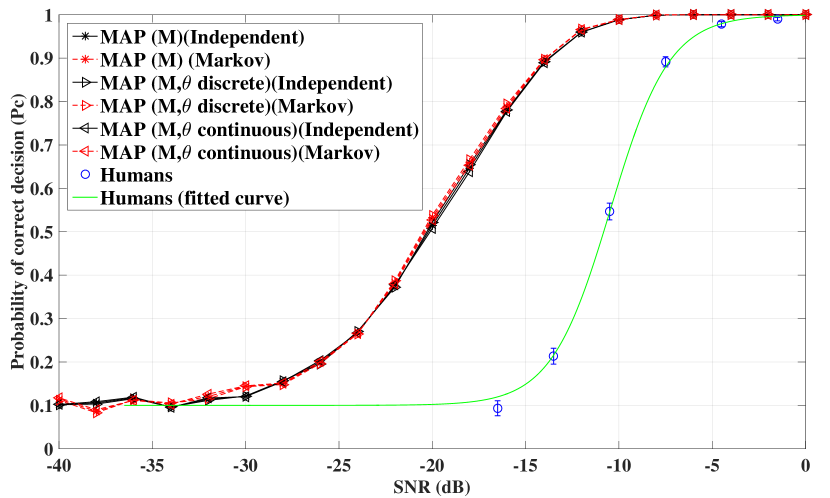
Figure 3: Performance of humans and the optimal classifiers for word recognition as a function of SNR. The error bars show the standard deviation of probability of correct decision among subjects.

Figure 4: Upper and lower bounds for the relative information loss $l_{I}$ in the human auditory system and the relative information loss in the optimal classifier as a function of SNR.

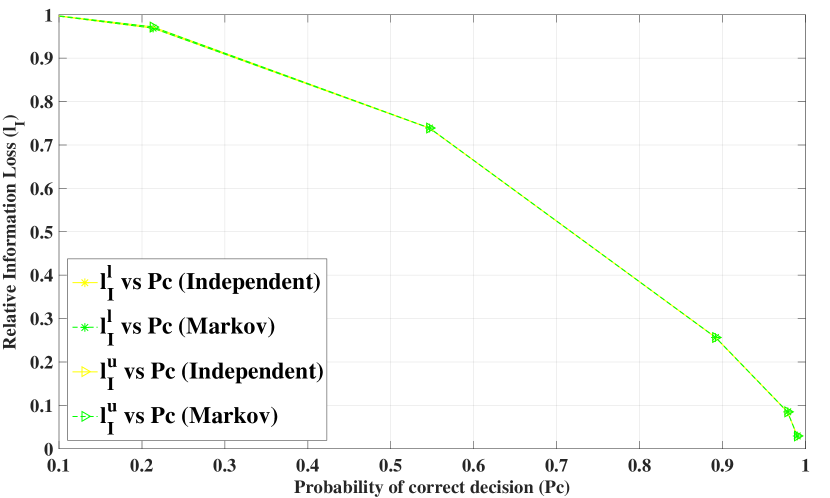
Figure 5: The relative information loss $l_{I}$ vs. probability of correct decision, $P_{c}$, for humans.

V Discussion

We observe from Fig. 3 that the word recognition rate for the classifiers and humans reach 1 at high SNRs, whereas at low SNRs, it is at the chance level $P_{c}=0.1$. This is because at high noise levels, the words are completely masked by noise, and both classifiers and humans choose words randomly from $\Gamma=10$ words. It can also be seen that the optimal classifiers perform almost identically, when we consider the Markov model of the first order compared to the optimal classifiers employing an independent-frame assumption. This implies that the independence assumption does not compromise the performance significantly. This result suggests that an independent-frame assumption, which is often employed in various speech processing contexts (e.g. [27]), is a reasonable assumption, at least in this context. The fact that the performances of all three classifiers are nearly identical, means that, in this test, the alphabet of the SNR and prior assumptions on it, are insignificant. Finally, we observe from Fig. 3 that machine performance is substantially better than human performance. In particular, the $50\%$ speech perception threshold for machine receivers is approximately $8$ dB lower than that of humans. The superior performance of classifiers for detecting noisy words compared to humans contradicts our hypothesis that humans are optimal at recognizing words in noise. In other words, the human auditory system performs sub-optimally in this particular task.

As can be seen from Fig. 4, the relative information loss at high SNRs ($\text{SNR}>-2\;\text{dB}$) for humans is around 0, whereas at low SNRs the relative information loss reaches its maximum 1. This is because for SNRs less than $-16$ dB, humans can not recognize the words and therefore simply guess; so in this case $I(M;M^{*})=0$ and $l_{I}=1$. We can therefore conclude that not only is less and less information available at the eardrum for decreasing SNRs, but of the information that is available at the eardrum, less and less is used for identifying the word. On the contrary, at high SNRs, there is no loss of the useful information needed for identifying the words in the human auditory system. It should be noted that the lower and upper bounds for the relative information loss for humans almost coincide. We also observe that the relative information loss in the optimal classifiers is less than the relative information loss in the human auditory system, which confirms that in this set-up, the human auditory system performs sub-optimally.

From Fig. 5, it is seen that there is an inverse relationship between probability of correct decision (or speech intelligibility) and the relative information loss for humans. This monotonic relationship between intelligibility and the amount of information that reaches the brain has also been observed in [28].

VI Conclusion

In this paper, we defined and quantified the information loss in the human auditory system. We first considered a speech communication model where words are spoken and sent through a noisy channel, and then received by a listener. For this setup, we defined and bounded the relative information loss in the listener. The relative information loss describes the fraction of speech information that reaches the eardrum of the listener, but which is not used to decode the speech. To obtain the word recognition rate for humans, we conducted a listening test. The results showed that bounds for the relative information loss in the human auditory system are tight and as SNR increases, the relative information loss decreases. We also assessed the hypothesis that whether humans are optimal in recognizing speech signals in noise. To do so, we derived optimal classifiers and compared their performance for information loss and word recognition rate to those of humans. The lower information loss and higher word recognition rate for machine classifiers compared to humans implied the sub-optimality of the human auditory system for recognizing noisy words, at least for speech contaminated by additive, Gaussian, speech-shaped noise.

Appendix A Proof of Lemma 1

Upper and lower bounds for the entropy of the mixture of distributions $f_{\textbf{Y}}(\textbf{y})=\sum_{m=1}^{\Gamma}P(M=m)f_{\textbf{Y}|m}(\textbf{y}|m)$ are obtained as [20]:

$$h_{l}(\textbf{Y})=h(\textbf{Y}|M)-\sum_{m=1}^{\Gamma}P(M=m)$$

$$\times \log\left(\sum_{m^{\prime}=1}^{\Gamma}P(M=m^{\prime})e^{-C_{\beta}(f_{\textbf{Y}|m}(\textbf{y}|m)||f_{\textbf{Y}|m^{\prime}}(\textbf{y}|m^{\prime}))}\right),$$

$$h_{u}(\textbf{Y})=h(\textbf{Y}|M)-\sum_{m=1}^{\Gamma}P(M=m)$$

$$\times \log\left(\sum_{m^{\prime}=1}^{\Gamma}P(M=m^{\prime})e^{-D_{KL}(f_{\textbf{Y}|m}(\textbf{y}|m)||f_{\textbf{Y}|m^{\prime}}(\textbf{y}|m^{\prime}))}\right),$$ (22)

where $h_{u}(\textbf{Y})$ and $h_{l}(\textbf{Y})$ denote the upper and lower bounds for $h(\textbf{Y})$ respectively. From (9), we have:

$$f_{\textbf{Y}|m}(\textbf{y})= \prod_{z=1}^{v}f_{\textbf{Y}_{z}|\textbf{y}^{z-1},m}(\textbf{y}_{z}|\textbf{y}^{z-1},m)$$ (23)

So the KL-divergence and the Chernoff $\beta$-divergence in (A) can be written as:

$$D_{KL}(f_{\textbf{Y}|m}||f_{\textbf{Y}|m^{\prime}})$$

$$=\sum_{z=1}^{v}E_{\textbf{y}^{z-1}}\left[D_{KL}(f_{\textbf{Y}_{z}|\textbf{y}^{z-1},m}||f_{\textbf{Y}_{z}|\textbf{y}^{z-1},m^{\prime}})\right],$$

$$C_{\beta}(f_{\textbf{Y}|m}||f_{\textbf{Y}|m^{\prime}})$$

$$=C_{\beta}(f_{\textbf{Y}^{v-1}|m}f_{\textbf{Y}_{v}|\textbf{y}^{v-1},m}||f_{\textbf{Y}^{v-1}|m^{\prime}}f_{\textbf{Y}_{v}|\textbf{y}^{v-1},m^{\prime}}).$$ (24)

Using (A) and the fact that $0\leq I(M;\textbf{Y})\leq H(M)=\log(\Gamma)$, we find a lower and upper bound for $I(M;\textbf{Y})$:

$$I_{l}(M;\textbf{Y})=\max\left\{0,h_{l}(\textbf{Y})-h(\textbf{Y}|M)\right\},$$

$$I_{u}(M;\textbf{Y})=\min\left\{\log(\Gamma),h_{u}(\textbf{Y})-h(\textbf{Y}|M)\right\}.$$ (25)

Using the result in (A) and substituting (A) in (A) completes our proof.

Appendix B Proof of lemma 2

Using Bayes’ theorem, the posterior probability can be written as [29]:

$$P(M=m|\textbf{y})=\dfrac{f_{\textbf{Y}|m}(\textbf{y}|m)P(M=m)}{f_{\textbf{Y}}(\textbf{y})}.$$ (26)

Since the speaker chooses words uniformly, $P(M=m)=\frac{1}{\Gamma},\forall m$, and $f_{\textbf{Y}}(\textbf{y})$ is independent of $M$, from (26), (18) can be rewritten:

$$m^{*}= \underset{m\in\{1,...,\Gamma\}}{\mathrm{arg}\mathrm{max}}\{P(M=m|\textbf{y})\}=$$

$$\underset{m\in\{1,...,\Gamma\}}{\mathrm{arg}\mathrm{max}}\{f_{\textbf{Y}|m}(\textbf{y}|m)\}.$$ (27)

In (23), we have obtained the PDF of $f_{\textbf{Y}|m}(\textbf{y}|m)$. However, the classifier does not know the SNR, $\theta$, so we can write:

$$f_{\textbf{Y}|m,\theta}(\textbf{y}|m,\theta)=\prod_{z=1}^{v}\dfrac{\mathcal{N}(\textbf{0},\mathbf{\Sigma}_{\textbf{Y}^{z}|m})}{\mathcal{N}(\textbf{0},\mathbf{\Sigma}_{\textbf{Y}^{z-1}|m})}.$$ (28)

Using (III-B1), we obtain:

$$\mathbf{\Sigma}_{\textbf{Y}^{z}|m}=\theta\mathbf{\Sigma}_{\textbf{X}_{m}^{z}}+\mathbf{\Sigma}_{\textbf{W}^{z}},$$

$$\mathbf{\Sigma}_{\textbf{Y}^{z-1}|m}=\theta\mathbf{\Sigma}_{\textbf{X}_{m}^{z-1}}+\mathbf{\Sigma}_{\textbf{W}^{z-1}}.$$ (29)

Using (28), we can calculate $f_{\textbf{Y}|m}(\textbf{y}|m)$ as:

$$f_{\textbf{Y}|m}(\textbf{y}|m)=\int f_{\textbf{Y}|m,\theta}(\textbf{y}|m,\theta)f_{\Theta}(\theta)d\theta$$

$$=\int\prod_{z=1}^{v}\dfrac{\mathcal{N}(\textbf{0},\mathbf{\Sigma}_{\textbf{Y}^{z}|m})}{\mathcal{N}(\textbf{0},\mathbf{\Sigma}_{\textbf{Y}^{z-1}|m})}\times f_{\Theta}(\theta)d\theta.$$ (30)

Since $\Theta\sim\mathcal{U}(a,b)$, we simply get:

$$m^{*}=\underset{m\in\{1,...,\Gamma\}}{\mathrm{arg}\mathrm{max}}\left\{\int_{a}^{b}\prod_{z=1}^{v}\dfrac{\mathcal{N}(\textbf{0},\mathbf{\Sigma}_{\textbf{Y}^{z}|m})}{\mathcal{N}(\textbf{0},\mathbf{\Sigma}_{\textbf{Y}^{z-1}|m})}\frac{1}{b-a}d\theta\right\}$$

$$=\underset{m\in\{1,...,\Gamma\}}{\mathrm{arg}\mathrm{max}}\int_{a}^{b}\left(\prod_{z=1}^{v}\dfrac{|2\pi\mathbf{\Sigma}_{\textbf{Y}^{z}|m}|^{-\frac{1}{2}}}{|2\pi\mathbf{\Sigma}_{\textbf{Y}^{z-1}|m}|^{-\frac{1}{2}}}\right)$$

$$\times\exp\frac{-1}{2}\sum_{z=1}^{v}\left((\textbf{y}^{z})^{T}\mathbf{\Sigma}_{\textbf{Y}^{z}|m}^{-1}\textbf{y}^{z}-\left(\textbf{y}^{z-1}\right)^{T}\mathbf{\Sigma}_{\textbf{Y}^{z-1}|m}^{-1}\textbf{y}^{z-1}\right)d\theta.$$ (31)

Appendix C Proof of Lemma 3

According to Bayes’ theorem, $f_{M,\Theta|\textbf{y}}(m,\theta|\textbf{y})$ can be written as:

$$f_{M,\Theta|\textbf{y}}(m,\theta|\textbf{y})=\dfrac{f_{\textbf{Y}|m,\theta}(\textbf{y}|m,\theta)f_{M,\Theta}(m,\theta)}{f_{\textbf{Y}}(\textbf{y})}.$$ (32)

Since $M$ and $\theta$ are mutually independent, it follows that $f_{M,\Theta}(m,\theta)=P(M=m)f_{\Theta}(\theta)=\frac{1}{\Gamma(b-a)}$. Using (32) and (28), (19) can then be expressed as:

$$(m^{*},\theta^{*})=\underset{m\in\{1,...,\Gamma\},\theta\in[a,b]}{\mathrm{arg}\mathrm{max}}\{f_{\textbf{Y}|m,\theta}(\textbf{y}|m,\theta)\},$$

$$=\underset{m\in\{1,...,\Gamma\},\theta\in[a,b]}{\mathrm{arg}\mathrm{max}}\left(\prod_{z=1}^{v}\dfrac{|2\pi\mathbf{\Sigma}_{\textbf{Y}^{z}|m}|^{-\frac{1}{2}}}{|2\pi\mathbf{\Sigma}_{\textbf{Y}^{z-1}|m}|^{-\frac{1}{2}}}\right)$$

$$\times\exp\frac{-1}{2}\sum_{z=1}^{v}\left((\textbf{y}^{z})^{T}\mathbf{\Sigma}_{\textbf{Y}^{z}|m}^{-1}\textbf{y}^{z}-\left(\textbf{y}^{z-1}\right)^{T}\mathbf{\Sigma}_{\textbf{Y}^{z-1}|m}^{-1}\textbf{y}^{z-1}\right).$$

By applying the logarithm, we get :

$$(m^{*},\theta^{*})=\underset{m\in\{1,...,\Gamma\},\theta\in[a,b]}{\mathrm{arg}\mathrm{max}}-\sum_{z=1}^{v}\left((\textbf{y}^{z})^{T}\mathbf{\Sigma}_{\textbf{Y}^{z}|m}^{-1}\textbf{y}^{z}\right.$$

$$\left.+\log|\mathbf{\Sigma}_{\textbf{Y}^{z}|m}|-\left(\textbf{y}^{z-1}\right)^{T}\mathbf{\Sigma}_{\textbf{Y}^{z-1}|m}^{-1}\textbf{y}^{z-1}-\log|\mathbf{\Sigma}_{\textbf{Y}^{z-1}|m}|\right).$$ (33)

Equation (C) indicates that the decoder chooses the pair $(m,\theta)$ maximizing

$$g=-\sum_{z=1}^{v}\left((\textbf{y}^{z})^{T}\mathbf{\Sigma}_{\textbf{Y}^{z}|m}^{-1}\textbf{y}^{z}+\log|\mathbf{\Sigma}_{\textbf{Y}^{z}|m}|\right.$$

$$\left.-\left(\textbf{y}^{z-1}\right)^{T}\mathbf{\Sigma}_{\textbf{Y}^{z-1}|m}^{-1}\textbf{y}^{z-1}-\log|\mathbf{\Sigma}_{\textbf{Y}^{z-1}|m}|\right).$$ (34)

Here $\textbf{y}^{z}$ and $\textbf{y}^{z-1}$ are assumed as constants at the decoder, so using that $\frac{\partial\log|\mathbf{\Sigma}_{\textbf{Y}^{z}|m}|}{\partial\theta}=\operatorname{tr}\left(\mathbf{\Sigma}_{\textbf{Y}^{z}|m}^{-1}\frac{\partial\mathbf{\Sigma}_{\textbf{Y}^{z}|m}}{\partial\theta}\right)$, and that $\frac{\partial\mathbf{\Sigma}_{\textbf{Y}^{z}|m}^{-1}}{\partial\theta}=-\mathbf{\Sigma}_{\textbf{Y}^{z}|m}^{-1}\frac{\partial\mathbf{\Sigma}_{\textbf{Y}^{z}|m}}{\partial\theta}\mathbf{\Sigma}_{\textbf{Y}^{z}|m}^{-1}$, we can find $\theta^{*}$ by taking the derivate of $g$ with respect to $\theta$ in the equation (C):

$$\dfrac{\partial g}{\partial\theta}=\sum_{z=1}^{v}\left(-(\textbf{y}^{z})^{T}\left(\mathbf{\Sigma}_{\textbf{Y}^{z}|m}^{-1}\mathbf{\Sigma}_{\textbf{X}_{m}^{z}}\mathbf{\Sigma}_{\textbf{Y}^{z}|m}^{-1}\right)\textbf{y}^{z}+\operatorname{tr}\left(\mathbf{\Sigma}_{\textbf{Y}^{z}|m}^{-1}\mathbf{\Sigma}_{\textbf{X}_{m}^{z}}\right)\right.$$

$$\left.+(\textbf{y}^{z-1})^{T}\left(\mathbf{\Sigma}_{\textbf{Y}^{z-1}|m}^{-1}\mathbf{\Sigma}_{\textbf{X}_{m}^{z-1}}\mathbf{\Sigma}_{\textbf{Y}^{z-1}|m}^{-1}\right)\textbf{y}^{z-1}\right.$$

$$\left.-\operatorname{tr}\left(\mathbf{\Sigma}_{\textbf{Y}^{z-1}|m}^{-1}\mathbf{\Sigma}_{\textbf{X}_{m}^{z-1}}\right)\right),$$

We obtain $\theta^{*}$ by solving $\dfrac{\partial g}{\partial\theta}=0$. Finally, $m^{*}$ is calculated as follows:

$$m^{*}=\underset{m\in\{1,...,\Gamma\}}{\mathrm{arg}\mathrm{max}}\left\{-\sum_{z=1}^{v}\left((\textbf{y}^{z})^{T}(\mathbf{\Sigma}_{\textbf{Y}^{z}|m}^{*})^{-1}\textbf{y}^{z}+\log|\mathbf{\Sigma}_{\textbf{Y}^{z}|m}^{*}|\right.\right.$$

$$\left.\left.-(\textbf{y}^{z-1})^{T}(\mathbf{\Sigma}_{\textbf{Y}^{z-1}|m}^{*})^{-1}\textbf{y}^{z-1}+\log|\mathbf{\Sigma}_{\textbf{Y}^{z-1}|m}^{*}|\right)\right\},$$

where

$$\mathbf{\Sigma}_{\textbf{Y}^{z}|m}^{*}=\theta^{*}\mathbf{\Sigma}_{\textbf{X}_{m}^{z}}+\mathbf{\Sigma}_{\textbf{W}^{z}},\mathbf{\Sigma}_{\textbf{Y}^{z-1}|m}^{*}=\theta^{*}\mathbf{\Sigma}_{\textbf{X}_{m}^{z-1}}+\mathbf{\Sigma}_{\textbf{W}^{z-1}}.$$

Appendix D Proof of Lemma 4

Using Bayes’ theorem, $P(M=m,\Theta=\theta_{i}|\textbf{y})$ can be expressed as:

$$P(M=m,\Theta=\theta_{i}|\textbf{y})=\dfrac{f_{\textbf{Y}|m,\theta_{i}}(\textbf{y}|m,\theta_{i})P(M=m,\Theta=\theta_{i})}{f_{\textbf{Y}}(\textbf{y})}.$$ (35)

Because $M$ and $\theta_{i}$ are mutually independent, $P(M,\Theta=\theta_{i})=P(M=m)P(\Theta=\theta_{i})=\frac{1}{\Gamma}\times\frac{1}{s}$. Using (35), (20) can be rewritten as:

$$(m^{*},i^{*})=\underset{m\in\{1,...,\Gamma\},i\in\{1,...,s\}}{\mathrm{arg}\mathrm{max}}\{f_{\textbf{Y}|m,\theta_{i}}(\textbf{y}|m,\theta_{i})\}.$$ (36)

Using (28), $f_{\textbf{Y}|m,\theta_{i}}$ is obtained as:

$$f_{\textbf{Y}|m,\theta_{i}}(\textbf{y}|m,\theta_{i})=\left(\prod_{z=1}^{v}\dfrac{|2\pi\mathbf{\Sigma}_{\textbf{Y}^{z}|m}^{i}|^{-\frac{1}{2}}}{|2\pi\mathbf{\Sigma}_{\textbf{Y}^{z-1}|m}^{i}|^{-\frac{1}{2}}}\right)$$

$$\times\exp\frac{-1}{2}\sum_{z=1}^{v}\left((\textbf{y}^{z})^{T}(\mathbf{\Sigma}_{\textbf{Y}^{z}|m}^{i})^{-1}\textbf{y}^{z}\right.$$

$$\left.-(\textbf{y}^{z-1})^{T}(\mathbf{\Sigma}_{\textbf{Y}^{z-1}|m}^{i})^{-1}\textbf{y}^{z-1}\right),$$

where

$$\mathbf{\Sigma}_{\textbf{Y}^{z}|m}^{i}=\theta_{i}\mathbf{\Sigma}_{\textbf{X}_{m}^{z}}+\mathbf{\Sigma}_{\textbf{W}^{z}},\mathbf{\Sigma}_{\textbf{Y}^{z-1}|m}^{i}=\theta_{i}\mathbf{\Sigma}_{\textbf{X}_{m}^{z-1}}+\mathbf{\Sigma}_{\textbf{W}^{z-1}}.$$

By applying the logarithm, the optimal pair $(m^{*},i^{*})$ is obtained as:

$$(m^{*},i^{*})=\!\!\!\!\!\!\!\!\!\!\!\!\!\!\!\!\underset{m\in\{1,...,\Gamma\},i\in\{1,...,s\}}{\mathrm{arg}\mathrm{max}}\!\!\!-\sum_{z=1}^{v}\left((\textbf{y}^{z})^{T}(\mathbf{\Sigma}_{\textbf{Y}^{z}|m}^{i})^{-1}\textbf{y}^{z}\right.$$

$$\left.+\log|\mathbf{\Sigma}_{\textbf{Y}^{z}|m}^{i}|-(\textbf{y}^{z-1})^{T}(\mathbf{\Sigma}_{\textbf{Y}^{z-1}|m}^{i})^{-1}\textbf{y}^{z-1}-\log|\mathbf{\Sigma}_{\textbf{Y}^{z-1}|m}^{i}|\right).$$

References

• [1] S. Seneff, “A joint synchrony/mean-rate model of auditory speech processing,” in Readings in speech recognition.   Morgan Kaufmann Publishers Inc., 1990, pp. 101–111.
• [2] O. Ghitza, “Auditory nerve representation as a front-end for speech recognition in a noisy environment,” Computer Speech & Language, vol. 1, no. 2, pp. 109–130, 1986.
• [3] R. F. Lyon, “A computational model of filtering, detection, and compression in the cochlea,” in Acoustics, Speech, and Signal Processing, IEEE International Conference on ICASSP’82., vol. 7.   IEEE, 1982, pp. 1282–1285.
• [4] J. Tchorz and B. Kollmeier, “A model of auditory perception as front end for automatic speech recognition,” The Journal of the Acoustical Society of America, vol. 106, no. 4, pp. 2040–2050, 1999.
• [5] T. Dau, D. Püschel, and A. Kohlrausch, “A quantitative model of the “effective”signal processing in the auditory system. i. model structure,” The Journal of the Acoustical Society of America, vol. 99, no. 6, pp. 3615–3622, 1996.
• [6] X. Yang, K. Wang, and S. A. Shamma, “Auditory representations of acoustic signals,” Information Theory, IEEE Transactions on, vol. 38, no. 2, pp. 824–839, 1992.
• [7] L. G. Huettel and L. M. Collins, “Using computational auditory models to predict simultaneous masking data: Model comparison,” Biomedical Engineering, IEEE Transactions on, vol. 46, no. 12, pp. 1432–1440, 1999.
• [8] L. H. Carney, “A model for the responses of low-frequency auditory-nerve fibers in cat,” The Journal of the Acoustical Society of America, vol. 93, no. 1, pp. 401–417, 1993.
• [9] W. M. Siebert, “Stimulus transformations in the peripheral auditory system,” Recognizing patterns, pp. 104–133, 1968.
• [10] R. D. Patterson, M. H. Allerhand, and C. Giguere, “Time-domain modeling of peripheral auditory processing: A modular architecture and a software platform,” The Journal of the Acoustical Society of America, vol. 98, no. 4, pp. 1890–1894, 1995.
• [11] T. Harczos, A. Chilian, and P. Husar, “Making use of auditory models for better mimicking of normal hearing processes with cochlear implants: The sam coding strategy,” Biomedical Circuits and Systems, IEEE Transactions on, vol. 7, no. 4, pp. 414–425, 2013.
• [12] K. Wagener, J. L. Josvassen, and R. Ardenkjær, “Design, optimization and evaluation of a danish sentence test in noise: Diseño, optimización y evaluación de la prueba danesa de frases en ruido,” International Journal of Audiology, vol. 42, no. 1, pp. 10–17, 2003.
• [13] W. Bialek, D. L. Ruderman, and A. Zee, “Optimal sampling of natural images: a design principle for the visual system,” in Advances in neural information processing systems, 1991, pp. 363–369.
• [14] J. J. Atick, “Could information theory provide an ecological theory of sensory processing?” Network: Computation in neural systems, vol. 3, no. 2, pp. 213–251, 1992.
• [15] F. Rieke, D. A. Bodnar, and W. Bialek, “Naturalistic stimuli increase the rate and efficiency of information transmission by primary auditory afferents,” Proceedings of the Royal Society of London B: Biological Sciences, vol. 262, no. 1365, pp. 259–265, 1995.
• [16] W. Bialek, M. DeWeese, F. Rieke, and D. Warland, “Bits and brains: Information flow in the nervous system,” Physica A: Statistical Mechanics and its Applications, vol. 200, no. 1-4, pp. 581–593, 1993.
• [17] W. Bialek, F. Rieke, R. R. de Ruyter van Steveninck, and D. Warland, “Reading a neural code,” Science, vol. 252, no. 5014, pp. 1854–1857, 1991.
• [18] T. M. Cover and J. A. Thomas, Elements of information theory.   John Wiley & Sons, 2012.
• [19] Rényi and Alfréd, “On measures of entropy and information,” in Proceedings of the Fourth Berkeley Symposium on Mathematical Statistics and Probability, Volume 1: Contributions to the Theory of Statistics.   The Regents of the University of California, 1961.
• [20] A. Kolchinsky and B. D. Tracey, “Estimating mixture entropy with pairwise distances,” arXiv preprint arXiv:1706.02419, 2017.
• [21] M. F. Huber, T. Bailey, H. Durrant-Whyte, and U. D. Hanebeck, “On entropy approximation for gaussian mixture random vectors,” in Multisensor Fusion and Integration for Intelligent Systems, 2008. MFI 2008. IEEE International Conference on.   IEEE, 2008, pp. 181–188.
• [22] T. Jebara and R. Kondor, “Bhattacharyya and expected likelihood kernels,” in Learning theory and kernel machines.   Springer, 2003, pp. 57–71.
• [23] H. Joe, “Estimation of entropy and other functionals of a multivariate density,” Annals of the Institute of Statistical Mathematics, vol. 41, no. 4, pp. 683–697, 1989.
• [24] M. R. Schädler, A. Warzybok, S. Hochmuth, and B. Kollmeier, “Matrix sentence intelligibility prediction using an automatic speech recognition system,” International Journal of Audiology, vol. 54, no. sup2, pp. 100–107, 2015.
• [25] R. M. Meyer and T. Brand, “Comparison of different short-term speech intelligibility index procedures in fluctuating noise for listeners with normal and impaired hearing,” Acta acustica united with Acustica, vol. 99, no. 3, pp. 442–456, 2013.
• [26] S. Godsill, “The restoration of degraded audio signals.” Ph.D. dissertation, University of Cambridge, 1993.
• [27] J. R. Deller Jr, J. G. Proakis, and J. H. Hansen, Discrete time processing of speech signals.   Prentice Hall PTR, 1993.
• [28] J. Jensen and C. H. Taal, “Speech intelligibility prediction based on mutual information,” IEEE/ACM Transactions on Audio, Speech and Language Processing (TASLP), vol. 22, no. 2, pp. 430–440, 2014.
• [29] J. G. Proakis, Digital communications.   New York: McGraw-Hill, 1995.