Marchenko method with incomplete data and singular nucleon scattering

We apply the Marchenko method of quantum inverse scattering to study nucleon scattering problems. Assuming a $\beta/r^{2}$ type repulsive core and comparing our results to the Reid93 phenomenological potential we estimate the constant $\beta$, determining the singularity strength, in various spin/isospin channels. Instead of using Bargmann type S-matrices which allows only integer singularity strength, here we consider an analytical approach based on the incomplete data method, which is suitable for fractional singularity strengths as well.

1 Introduction and motivation

The characteristic features of the phenomenological nucleon potentials [1, 2, 3], shown in Fig. 1, are well known. The force at medium to long range is attractive; this feature is due to pion and other heavier meson exchange. The strong repulsive core of the potential at short distances had no satisfactory theoretical explanation until recent advances in lattice QCD simulations made possible to determine the potential in fully dynamical lattice QCD [4, 5]. The results of this first principles calculation resemble the phenomenological potential, including its repulsive core. The short distance behaviour of the potential was subsequently studied also in perturbative QCD. The results of the perturbative calculations [6, 7] show that at extremely short distances the potential behaves as $1/r^{2}$ (up to log corrections characteristic to perturbative QCD). Calculations in holographic QCD [8] also give a similar inverse square potential at short distances.

Although the recent theory of low energy nuclear interactions is based on effective chiral field theory (EFT) of mesons and nucleons (for a review, see [9]), the phenomenological potential remains important as a source of intuition and is still often used in the study of multinucleon systems and in the determination of the equation of state for dense nuclear matter as starting point of quantitative work.

As can be seen in Fig. 1, the phenomenological potential is not uniquely determined. Nevertheless, known versions more or less agree on its main qualitative features at large and medium distances and substantially deviate only at short distances (corresponding to higher energies). From a purist viewpoint the notion of nuclear potential does not make much sense much below 0.5 fermi for various reasons: the nonrelativistic quantum-mechanical description based on the Schrödinger equation cannot work beyond about 350 MeV laboratory (LAB) energy because it cannot incorporate particle production; relativistic effects become important at the corresponding energy range; finally the composite nature of nucleons becomes relevant at distances comparable to their size. (By using EFT, which is a relativistic quantum field theory, the first two difficulties are avoided but it cannot directly address the last problem either.) Therefore a meaningful reconstruction of an effective nuclear potential (more precisely a Hamilton operator in the Schrödinger equation) must be based on experimental data in the $0<E_{\rm LAB}<350\ {\rm MeV}$ energy range. This leads to the problem of quantum inverse scattering with incomplete data.

We have investigated [10] analogous problems in the $1+1$ dimensional Sine-Gordon model. Since this relativistic model is integrable, there is no particle production, but we can still ask the question whether an effective potential exists which exactly reproduces the known scattering phase shifts. We found that the answer is affirmative both in the centre of mass (COM) and the LAB frame, but the price one has to pay is frame-dependence. However, we also found that in this model the frame-dependence is weak, both at small and large distances and the COM and LAB frame effective potentials are qualitatively similar and numerically close also at medium distance. Thus an approximate notion of effective potential makes sense, at least in this model.

In the theory of inverse scattering with incomplete data the lack of full information on the scattering phase shifts is (partially) compensated by other, additional pieces of information. In this paper we concentrate on the singular core of the potential and assume it behaves for small $r$ as

$$U(r)\sim\frac{\nu(\nu+1)}{r^{2}}+{\rm O}(1)$$ (1.1)

(in natural units), where the parameter $\nu$ is non-negative (repulsive core). In a recent paper [11] we studied the singular behaviour of the nucleon potential in the ${}^{1}S_{0}$ channel and in the ${}^{3}S_{1}$-${}^{3}D_{1}$ coupled channels. Assuming a rational, Bargmann-type S-matrix, a (1.1)-type small $r$ asymptotic behaviour naturally emerges. In this method the incompleteness of the scattering data is compensated by the assumption on the rational form of the S-matrix. For Bargmann-type S-matrices the strength parameter $\nu$ can only take integer values. By making comparisons to phenomenological potentials we found that $\nu=2$ in the ${}^{1}S_{0}$ channel and $\nu=1$, $\nu=3$ correspond to the ${}^{3}S_{1}$ and ${}^{3}D_{1}$ channels, respectively (up to small mixing effects).

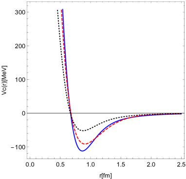
Figure 1: The phenomenological nucleon potential in the ${}^{1}S_{0}$ channel. The solid (blue) line is the AV18 fit [2], the dashed (red) line is the Reid93 fit [1] and the dotted line (black) is the CDBonn potential [3].

However, on physical grounds, there is no reason why the effective strength parameter $\nu$ should be integer. In this paper we undertake a systematic study of the strength parameter $\nu$ in various $np$ scattering channels assuming the form (1.1) but not requiring $\nu$ integer. We use the Marchenko method of quantum inverse scattering because this efficient method is applicable to all type of potentials (not necessarily of Bargmann-type). In case of Bargmann potentials the Marchenko method has the extra advantage that the results can be obtained purely algebraically [11]; in other cases it requires the solution of a linear integral equation.

Quantum inverse scattering, the problem of finding the potential from scattering data, is completely solved in the one-dimensional case [12, 13, 14] in a mathematically precise way. The same mathematical problem emerges for three-dimensional spherically symmetric potentials after partial wave expansion. The potential can be uniquely reconstructed, in a given class of potentials, if full information on scattering at all energies and some additional data related to bound states (binding energies and asymptotic decay constants) are all available. Since this is rarely the case, the method has not been used often [15] in nuclear theory, except in the case of Bargmann-type potentials [16, 17].

First, using the methods of [18], we slightly generalized existing results to incorporate singular potentials. Secondly, we worked out a method to extrapolate limited range data so that the resulting potential is of the form (1.1). This is possible because the asymptotic large energy behaviour is intimately related to the singularity strength via the generalized Levinson’s theorem.

We tested our method on an exactly solvable generalized Pöschl-Teller (Bargmann-type) potential, a slight generalization of those studied in [19]. We found that the correct $\nu$ can be reproduced with reasonable precision with our method.

Finally we undertook a systematic study of the $\nu$ parameter for various low angular momentum partial waves of $np$ scattering: in the ${}^{1}S_{0}$, ${}^{3}P_{1}$, ${}^{3}P_{0}$ and ${}^{3}D_{2}$ channels. We constructed the potential in each channel with a (1.1) type singular behaviour based on experimental data below 350 MeV LAB energy and extrapolated with some fixed $\nu$. We decided to compare the resulting potential to the Reid93 phenomenological potential [1] at each channel, since it is a better description [20] of post-1993 data than the alternative AV18 [2] phenomenological potential. We determined the best choice for $\nu$ by requiring it gives the best fit in the energy range 500-1000 MeV, somewhat above the validity range of the original experimental data. We found that the singularity of the central potential in the ${}^{1}S_{0}$ channel is still best approximated by $\nu=2.0$, an integer. (Visible deviations appear if we choose $\nu=1.8$ or $\nu=2.2$.) But the best choice for the ${}^{3}P_{1}$, ${}^{3}P_{0}$, ${}^{3}D_{2}$ channels turn out to be $\nu=2.3$, $\nu=3.2$, $\nu=2.3$, respectively.

As discussed above, the strength of the repulsive core (and the precise shape of the attraction pocket) depends on the particular choice of the phenomenological potential and this leads to a corresponding ambiguity in the determination of our strength parameter $\nu$. Since our favourite choice (the Reid93 parametrization) is just one particular choice, in the case of some channels (where both are available) we made a study of $\nu$ values obtained by comparison to the AV18 parametrization. We found that the optimal $\nu$ values differ only slightly between the two determinations.

The paper is organized as follows. In the next section we summarize Marchenko’s quantum inverse scattering algorithm. In section 3 we present our extrapolation method for singular potentials, which is then applied in the next two sections to $np$ scattering in various low angular momentum partial waves. Our conclusions are summarized in section 6.

2 Marchenko method of inverse scattering

In this paper we will apply the Marchenko method of inverse scattering to $np$ scattering problems. Since our main focus is the singularity strength of the repulsive core of the potential, we have generalized the theory of quantum inverse scattering to the case of singular potentials (see [11]).

Our starting point is the radial Schrödinger equation

$$-\frac{\hbar^{2}}{2m}u^{\prime\prime}(r)+\frac{\hbar^{2}}{2m}\,\frac{\ell(\ell+1)}{r^{2}}u(r)+V(r)u(r)=Eu(r),$$ (2.1)

where $m$ is the reduced mass, $V$ is the interaction potential and $E$ is the total energy of the particles. We introduce

$$q(r)=\frac{2m}{\hbar^{2}}V(r),\qquad k^{2}=\frac{2mE}{\hbar^{2}},\qquad U(r)=q(r)+\frac{\ell(\ell+1)}{r^{2}},$$ (2.2)

which allows us to simplify (2.1) as

$$-u^{\prime\prime}(r)+U(r)u(r)=k^{2}u(r).$$ (2.3)

We will consider potentials which are singular at the origin and vanish exponentially at large distances,

$$q(r) \sim \frac{\beta_{o}}{r^{2}}+{\rm O}(1),\qquad\quad\quad r\to 0,$$ (2.4)

$$q(r) \sim e^{-2\kappa r},\qquad\quad r\to\infty,\quad(\kappa>0).$$ (2.5)

The small $r$ singularity of the total potential term in (2.3) is determined by the parameter $\nu$ defined by

$$\nu(\nu+1)=\beta_{o}+\ell(\ell+1).$$ (2.6)

Quantum inverse scattering is a method to reconstruct the potential from scattering data. The latter is the set

$$\big{\{}S(k),0<k<\infty;\{s_{j},\kappa_{j}\}_{j=1}^{J}\big{\}},$$ (2.7)

where $S(k)=\exp\{2i\delta(k)\}$ is the S-matrix. We see that we not only need the phase shift $\delta(k)$ for all energies (all momenta $k$), but also additional bound state information $\{s_{j},\kappa_{j}\}$ for all bound states $j=1,\dots,J$. Here $\kappa_{j}$ is related to the binding energy by

$$E_{j}=-\frac{\hbar^{2}\kappa_{j}^{2}}{2m}$$ (2.8)

and $s_{j}$ to the asymptotic decay constant of the normalized bound state wave function $\psi_{j}(r)$ by

$$s_{j}=A_{j}^{2},\qquad\qquad\psi_{j}(r)\sim A_{j}{\rm e}^{-\kappa_{j}r},\qquad r\to\infty.$$ (2.9)

The set of scattering data is only restricted by the requirement

$$\delta(k)={\rm O}(k^{2\ell+1}),\qquad k\to 0$$ (2.10)

(in the convention $\delta(0)=0$), and that the singularity strength $\nu$, calculated from the generalized Levinsons’s theorem [11],

$$\nu=\frac{2}{\pi}[\delta(0)-\delta(\infty)]-2J+\ell,$$ (2.11)

must be non-negative (repulsive core).

If all scattering data are available, we first have to construct Marchenko’s $F(r,s)$ function, which is the sum of a bound state contribution and a scattering contribution.

$$F(r,s)=F_{\rm bound}(r,s)+F_{\rm scatt}(r,s),$$ (2.12)

where

$$F_{\rm bound}(r,s)=(-1)^{\ell+1}\sum_{j=1}^{J}s_{j}\ h_{\ell}(i\kappa_{j}r)\ h_{\ell}(i\kappa_{j}s),$$ (2.13)

and

$$\begin{split}&F_{\rm scatt}(r,s)=-\frac{\sin\nu\pi}{\pi(r+s)}+\frac{1}{2\pi}\int_{0}^{\infty}{\rm d}k\,\Big{\{}[S(k)-1]h_{\ell}(kr)h_{\ell}(ks)+[S(-k)-1]h_{\ell}(-kr)h_{\ell}(-ks)\\ &+[1-S(\infty)](-1)^{\ell+1}\,{\rm e}^{ik(r+s)}+[1-S(-\infty)](-1)^{\ell+1}\,{\rm e}^{-ik(r+s)}\Big{\}}.\end{split}$$ (2.14)

Here $h_{\ell}(x)$ is the Riccati-Hankel function, defined as

$$h_{\ell}(x)=(-i)^{\ell+1}e^{ix}\sum^{\ell}_{m=0}\frac{i^{m}}{m!(2x)^{m}}\frac{(\ell+m)!}{(\ell-m)!}.$$ (2.15)

The scattering part can be rewritten after partial integration as

$$F_{\rm scatt}(r,s)=\frac{2}{\pi}(-1)^{\ell}\frac{1}{r+s}\int_{0}^{\infty}{\rm d}k\,\delta^{\prime}(k){\rm Re}\,\left\{S(k){\rm e}^{ik(r+s)}R_{\ell}(r,s,k)\right\},$$ (2.16)

where

$$R_{\ell}(r,s,k)=\frac{1}{s-r}\left[sP_{\ell}(kr)P_{\ell-1}(ks)-rP_{\ell}(ks)P_{\ell-1}(kr)\right]$$ (2.17)

and $P_{\ell}$ is the polynomial part of the Hankel function (2.15):

$$P_{\ell}(x)=\sum_{m=0}^{\ell}C_{\ell,m}\left(\frac{i}{x}\right)^{m},\qquad\quad C_{\ell,m}=\frac{(\ell+m)!}{2^{m}m!(\ell-m)!}.$$ (2.18)

After some algebra, we can write

$$R_{\ell}(r,s,k)=\sum_{m=0}^{\ell}C_{\ell,m}\frac{Z_{m}(-i(r+s)k)}{(-rsk^{2})^{m}},$$ (2.19)

where $Z_{m}(\xi)$ is a polynomial of degree $m$. The first few polynomials are

$$Z_{0}(\xi)=1,\qquad Z_{1}(\xi)=\xi,\qquad Z_{2}(\xi)=\xi(\xi+1),\qquad Z_{3}=\xi(\xi^{2}+3\xi+3)$$ (2.20)

and

$$Z_{4}=\xi(\xi^{3}+6\xi^{2}+15\xi+15).$$ (2.21)

This gives

$$R_{0}(r,s,k) = 1,$$ (2.22)

$$R_{1}(r,s,k) = 1+\frac{i(r+s)}{rsk},$$ (2.23)

$$R_{2}(r,s,k) = 1+\frac{3i(r+s)}{rsk}-\frac{3i(r+s)}{(rs)^{2}k^{3}}-\frac{3(r+s)^{2}}{(rs)^{2}k^{2}},$$ (2.24)

etc. (2.19) is most convenient for numerical integration because it reduces the calculation of Marchenko’s $F$, a function of two variables, to the calculation of $\ell+1$ functions of one variable.

The next step is to solve the Marchenko equation

$$F(r,s)+A(r,s)+\int_{r}^{\infty}A(r,u)F(u,s)\,{\rm d}u=0,\qquad\quad s\geq r$$ (2.25)

for $A(r,s)$. Finally one has to take the derivative of $A(r,r)$ and obtain the potential in the Schrödinger equation (2.3) by

$$q(r)=-2\frac{{\rm d}}{{\rm d}r}\,A(r,r),\quad\qquad U(r)=q(r)+\frac{\ell(\ell+1)}{r^{2}}.$$ (2.26)

3 Singular potentials and incomplete data

Marchenko’s method is useful only if we have access to the full set of scattering data (2.7). In our case of the nonrelativistic nucleon potential, as explained in the introduction, for various reasons we can only use low energy data up to about 350 MeV LAB energy. Since for the uncoupled channels we are considering there are no bound states, the only missing piece is scattering phase shifts for energies above the maximal energy, which we take to be 350 MeV.

In this paper we adopted the following strategy. We use measured phase shifts up to the maximal energy and smoothly extrapolate this function for higher energies taking into account the singularity strength of the potential, which, in the absence of bound states, is related to the asymptotic value of the phase shift by the relation

$$\delta(\infty)=-\frac{\pi}{2}(\nu-\ell).$$ (3.1)

In more detail, we use as our phase shift

$$\delta(k)=\left\{\begin{split}&\delta_{\rm int}(k),\qquad 0<k<k_{o},\\ &\delta_{\rm ext}(k),\qquad k>k_{o},\end{split}\right.$$ (3.2)

where $\delta_{\rm int}$ is an interpolating function based on the measured data points with the only constraint

$$\delta_{\rm int}(k)={\rm O}(k^{2\ell+1})$$ (3.3)

for small $k$, and $\delta_{\rm ext}$ is the extrapolated part with

$$\delta_{\rm ext}(\infty)=-\frac{\pi}{2}(\nu-\ell)$$ (3.4)

asymptotics. Moreover, at the point $k=k_{o}=2.054\,{\rm fm}^{-1}$, which corresponds to the maximal energy, we require that the interpolation and the extrapolation are joined smoothly. We made the simple choice

$$\delta_{ext}(k)=-\frac{\pi}{2}(\nu-\ell)+\sum_{m=1}^{3}\frac{a_{m}}{k^{m}}$$ (3.5)

and determined the three constants $a_{m}$ from the requirements that the value, the slope and the curvature of the two functions coincide at $k=k_{o}$.

In the next subsection we study a test example, which shows that this simple method work reasonably well, at least in the class of functions resembling the phenomenological nucleon potential.

3.1 A test example

To test our method we have chosen the $\ell=0$ phase shift

$$\delta_{\rm exact}(k)=-\pi+\sum_{n=1}^{6}\arctan\left(\frac{x_{n}}{k}\right),$$ (3.6)

where

$$x_{1}=-0.0401,x_{2}=-0.7540,x_{3}=0.6152,x_{4}=2.0424,x_{5}=4.1650,x_{6}=4.6000.\quad$$ (3.7)

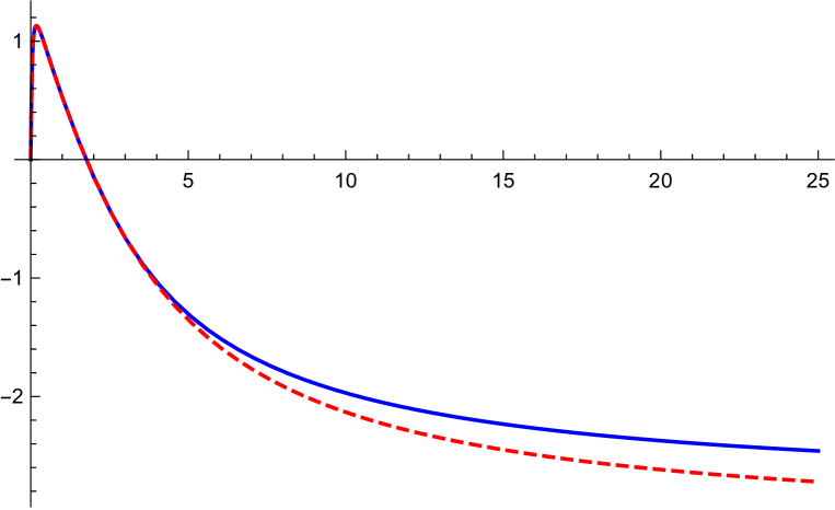
(a) $\nu=1.8$

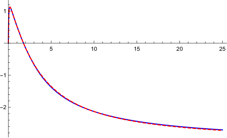
(b) $\nu=2.0$

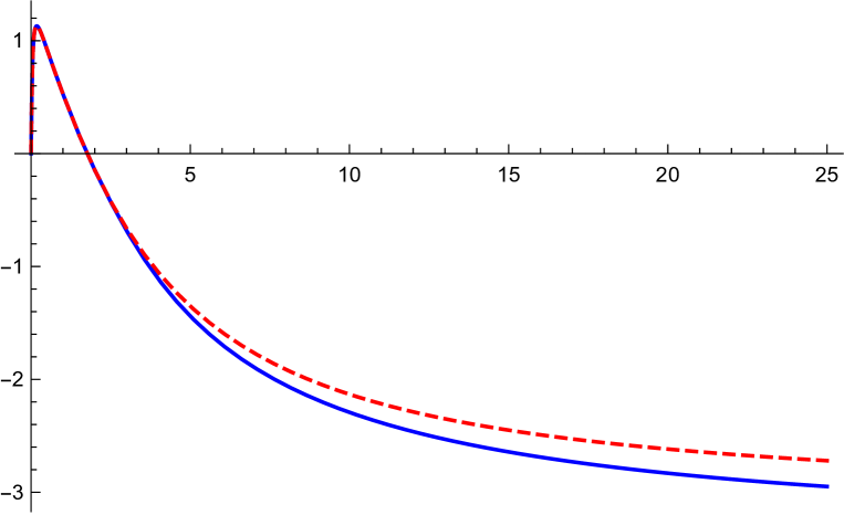
(c) $\nu=2.2$

Figure 2: Reconstruction of the phase shift $\delta(k)$ (radian) with different singularity strength values. The solid (blue) line is the phase shift obtained with our extrapolation method and the dashed (red) line is the original phase shift. The extrapolation starts at $k=2$.

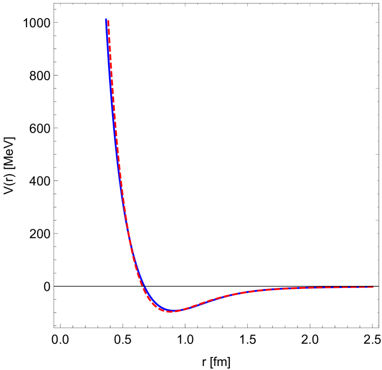
(a) $\nu=1.8$

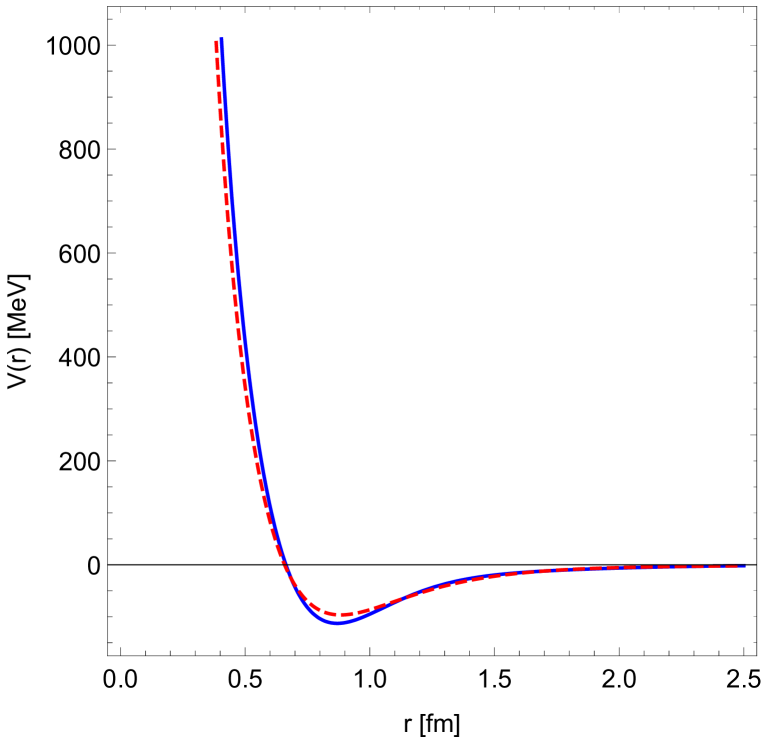
(b) $\nu=2.2$

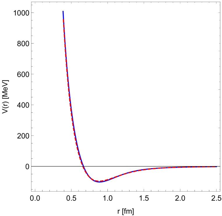
(c) $\nu=2.0$

Figure 3: Reconstruction of the test potential with different singularity strength values. The solid (blue) line is the potential obtained with our extrapolation method and the dashed (red) line is the original test potential.

Assuming the absence of bound states, from Levinson’s theorem we see that this phase shift corresponds to a Bargmann-type S-matrix with $\nu=2$. The parameter values are from [21] and we also used this Bargmann S-matrix in [11] to represent the phenomenological potential for $np$ scattering in the ${}^{1}S_{0}$ channel. However, for our present purposes it just serves as an exactly known test potential, which is qualitatively similar to the nucleon phenomenological potential.

To mimic what we want to do in the real case later, we approximate the phase shift as

$$\delta(k)=\left\{\begin{split}&\delta_{\rm exact}(k),\qquad 0<k<2,\\ &\delta_{\rm ext}(k),\qquad\qquad k>2,\end{split}\right.$$ (3.8)

where the extrapolation is of the form (3.5) and the two parts are glued together at $k=2$ requiring that the values, slopes and curvatures match at that point.

We have considered the values $\nu=1.8$, $\nu=2.0$ and $\nu=2.2$. The reconstruction of the potential for the original, Bargmann-type phase shift (3.6) is of course already known [21, 11]. For the extrapolated phase shifts we calculated both Marchenko’s $F$ function and the solution of the Marchenko equation numerically. The extrapolated phase shifts are compared to the original in Fig. 2, while the potential reconstructed with the Marchenko method is shown in Fig. 3. As we can see, for $\nu=1.8$ and $\nu=2.2$ some deviation (with opposite sign) is clearly visible, while for the true value $\nu=2.0$ the agreement of our extrapolated phase shift and potential with the original is quite good. We can conclude that our extrapolation method works reasonably well and the “true” value of the singularity strength $\nu$ can be estimated.

4 ${}^{1}S_{0}$ channel as an example of inverse scattering with incomplete data

In this section we apply our extrapolation method to the central potential in the ${}^{1}S_{0}$ isovector channel.

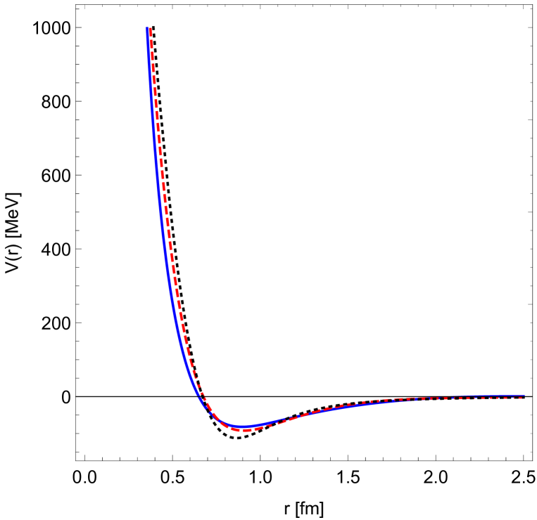
(a) $\nu=1.8$

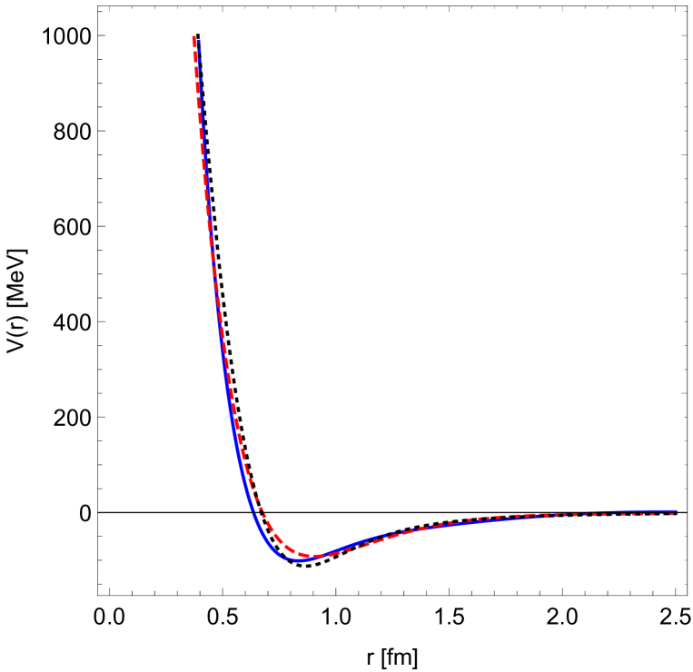
(b) $\nu=2.2$

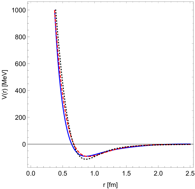
(c) $\nu=2.0$

Figure 4: Reconstruction of the ${}^{1}S_{0}$ channel central potential with different singularity strength values. The solid (blue) line is the potential obtained with our extrapolation method and the dashed (red) line is the Reid93 [1] potential. For comparison, the AV18 potential [2] is also shown (dotted, black).

For this purpose we downloaded the phase shifts from the publicly available GWDAC data base [22]. We use 35 phase shift data for LAB energies between 0 and 350 MeV. For concreteness, we have chosen the results of the analysis of Ref. [23] (unweighted fit). Of course, these results are already processed and not raw experimental data but for simplicity we call them ‘experimental’ data. The results of other phase shift analyses differ very little from these, in the potential model region we are studying.

Next we constructed our phase shift function by smoothly gluing together the interpolation to the experimental data with the extrapolation for higher energies as explained in section 3. Because in our previous study [11] based on Bargmann-type extrapolation we found that $\nu=2$ gives satisfactory results, we have considered the parameter values $\nu=1.8$, $\nu=2.0$ and $\nu=2.2$ here.

Having constructed our $\delta(k)$, we calculated Marchenko’s $F$ function numerically using the formula (see (2.16), (2.22))

$$F_{0}(r,s)=F_{(0)}(x)=\frac{2}{\pi x}\int_{0}^{\infty}{\rm d}k\,\delta^{\prime}(k)\cos[2\delta(k)+kx],$$ (4.1)

where $x=r+s$. There is no bound state contribution in this problem.

Finally we solved the Marchenko integral equation (2.25) numerically. The calculation is greatly simplified by noticing that for every fixed $r$ we have a separate problem, parametrized by $r$, where only the $s$ variable is dynamical.

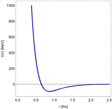
Figure 5: Comparison of the reconstructed ${}^{1}S_{0}$ channel potential at $\nu=2.0$ (solid, blue) to the Bargmann-type potential (dotted, black).

The results are shown in Fig. 4. Here we compare our potentials, reconstructed by the Marchenko method from our extrapolated phase shifts, for the three different strength parameter values with the Reid93 [1] phenomenological potential. (In the plots the alternative AV18 [2] phenomenological potential is also shown.) The figure suggests that $\nu=2.0$ is the best choice here. For $\nu=1.8$ and $\nu=2.2$ there is already a noticable deviation (in opposite directions) from Reid93 in the high energy range above 500 MeV. Thus our conclusion is that the integer value $\nu=2$ found previously in the class of Bargmann potentials remains the best choice here, even if we allow for non-integer values of the parameter. Actually, the potential reconstructed by the above method and the Bargmann potential differ by very little, as shown in Fig. 5. $\nu=2$ corresponds to $\beta_{o}=6$ in (2.6).

5 Other channels

5.1 The ${}^{3}P_{1}$, ${}^{3}P_{0}$ and ${}^{3}D_{2}$ channels

We have also studied the potentials corresponding to the uncoupled channels ${}^{3}P_{1}$, ${}^{3}P_{0}$ and ${}^{3}D_{2}$ with the same method.

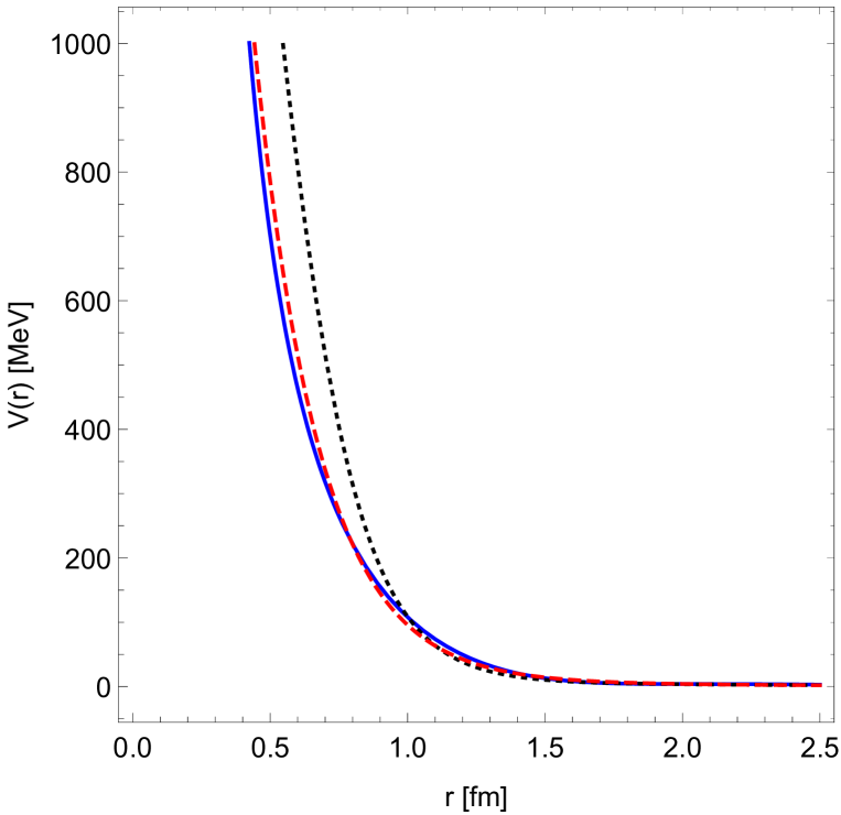
(a) $\nu=2.1$

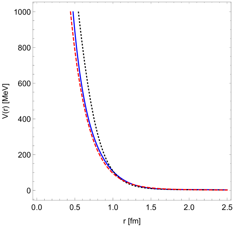
(b) $\nu=2.5$

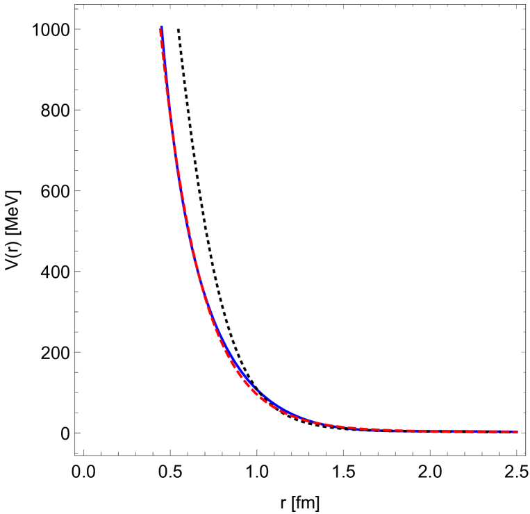
(c) $\nu=2.3$

Figure 6: Reconstruction of the ${}^{3}P_{1}$ channel nucleon potential with different singularity strength values. The solid (blue) line is the potential obtained with our extrapolation method and the dashed (red) line is the Reid93 [1] potential. For comparison, the AV18 potential [2] is also shown (dotted, black).

For ${}^{3}P_{1}$ and ${}^{3}P_{0}$ the angular momentum is $\ell=1$ and we have the constraint that the interpolating function near $k=0$ has to be ${\rm O}(k^{3})$. Marchenko’s $F$ function is given by the formula (see (2.16), (2.23))

$$F_{1}(r,s)=-F_{(0)}(x)-\frac{F_{(1)}(x)}{rs},$$ (5.1)

where $F_{(0)}$ is given by (4.1),

$$F_{(1)}(x)=-\frac{2}{\pi}\int_{0}^{\infty}\frac{{\rm d}k}{k}\delta^{\prime}(k)\sin[2\delta(k)+kx]$$ (5.2)

and $x=r+s$.

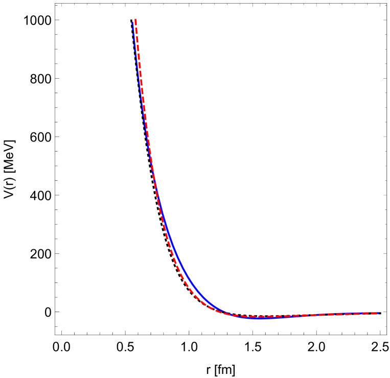
(a) $\nu=3.0$

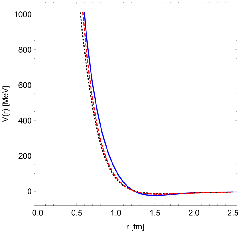
(b) $\nu=3.4$

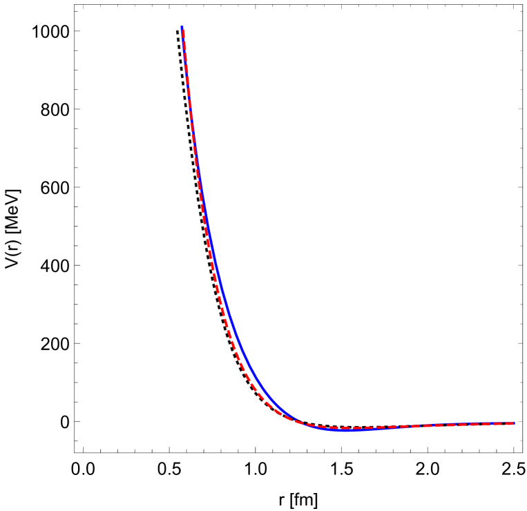
(c) $\nu=3.2$

Figure 7: Reconstruction of the ${}^{3}P_{0}$ channel nucleon potential with different singularity strength values. The solid (blue) line is the potential obtained with our extrapolation method and the dashed (red) line is the Reid93 [1] potential. For comparison, the AV18 potential [2] is also shown (dotted, black).

For ${}^{3}D_{2}$ $\ell=2$ and the constraint is $\delta(k)={\rm O}(k^{5})$. Marchenko’s $F$ function is given by (see (2.16), (2.24))

$$F_{2}(r,s)=F_{(0)}(x)+3\frac{F_{(1)}(x)}{rs}+3\frac{F_{(2)}(x)}{(rs)^{2}},$$ (5.3)

where $F_{(0)}$ is given by (4.1), $F_{(1)}$ by (5.2) and

$$F_{(2)}(x)=\frac{2}{\pi}\int_{0}^{\infty}{\rm d}k\,\delta^{\prime}(k)\Big{\{}\frac{\sin[2\delta(k)+kx]}{k^{3}}-\frac{x\cos[2\delta(k)+kx]}{k^{2}}\Big{\}}.$$ (5.4)

channel	$\ell$ value	best fit $\nu$ value	$\beta_{o}$ value
${}^{1}S_{0}$	0	2.0	6.0
${}^{3}P_{1}$	1	2.3	5.6
${}^{3}P_{0}$	1	3.2	11.4
${}^{3}D_{2}$	2	2.3	1.6

Table 1: Fractional $\nu$ values and the corresponding $\beta_{o}$ values

The results are shown in Figs. 6, 7 and 8. We found that for ${}^{3}P_{1}$ the best fit is $\nu=2.3$ (we also considered the neighbouring values $\nu=2.3\pm 0.2$). Similarly, for ${}^{3}P_{0}$ the best value is $\nu=3.2$ and in the plots the neighbouring $\nu=3.2\pm 0.2$ values are also shown. Finally for ${}^{3}D_{2}$ we have chosen $\nu=2.3$, $\nu=2.3\pm 0.1$.

As expected, there is no reason why the effective strength parameter $\nu$ should be integer. Indeed, in all our examples the best choice turns out to be fractional. We summarize our results for the best $\nu$ and the corresponding $\beta_{o}$ values in Table 1.

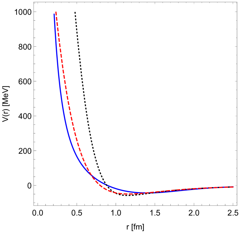
(a) $\nu=2.2$

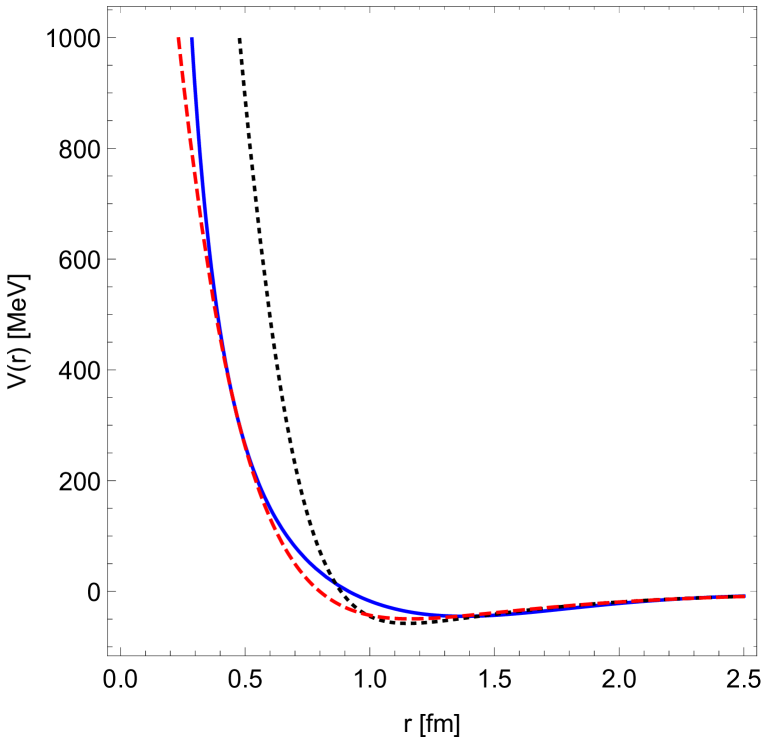
(b) $\nu=2.4$

(c) $\nu=2.3$

Figure 8: Reconstruction of the ${}^{3}D_{2}$ channel nucleon potential with different singularity strength values. The solid (blue) line is the potential obtained with our extrapolation method and the dashed (red) line is the Reid93 [1] potential. For comparison, the AV18 potential [2] is also shown (dotted, black).

5.2 An overall picture

The nonrelativistic Hamiltonian describing the nucleon-nucleon interaction is traditionally [24] written as a sum of three terms:

$$V(r)=V_{\rm C}(r)+V_{\rm T}(r)S_{12}+V_{\rm SO}(r)\vec{S}\cdot\vec{L},$$ (5.5)

where

$$S_{12}=3(\vec{\sigma}_{1}\cdot\vec{r}_{o})(\vec{\sigma}_{2}\cdot\vec{r}_{o})-(\vec{\sigma}_{1}\cdot\vec{\sigma}_{2})$$ (5.6)

is the tensor operator with $\vec{\sigma}_{1,2}$ the sigma matrices in the spin space of particles 1, 2 and $\vec{r}_{o}$ is the unit vector along the line connecting the two particles. $\vec{S}\cdot\vec{L}$ is the spin-orbit interaction operator. Later more operators were considered, like in the Argonne potentials AV14, AV18 [2], but here we use this simple form and further assume that only the central and tensor potentials are singular and the total singularity strength is described by the formula

$$\beta_{o}=A_{ST}-B_{T}S_{12}$$ (5.7)

with the constant $A_{ST}$ depending on the total spin and isospin and the constant $B_{T}$ depending only on isospin (since for $S=0$ the tensor operator vanishes). The tensor potential needs to be singular, since only the tensor operator $S_{12}$ has off-diagonal matrix elements in the case of coupled channels and the singularity of off-diagonal matrix elements of the potential is observed, for example, in the ${}^{3}S_{1}$-${}^{3}D_{1}$ coupled problem.

The matrix elements of $S_{12}$ are as follows. For the $S=0$ uncoupled channels ($J=\ell$) $S_{12}=0$. For the $S=1$ uncoupled channels ($J=\ell$) $S_{12}=2$. For the coupled channels the formulas are generally more complicated, for example, for the ${}^{3}S_{1}$-${}^{3}D_{1}$ channel, in the $\ell=(0,2)$ basis the matrix elements are

$$\begin{pmatrix}0&\sqrt{8}\\ \sqrt{8}&-2\end{pmatrix}.$$ (5.8)

Finally, for the exceptional uncoupled channel ${}^{3}P_{0}$, $S_{12}=-4$. We summarize these data in Table 2.

channel	$\beta_{o}$ value	$S/T$ values	$S_{12}$ values
${}^{1}S_{0}$	6.0	0/1	0
${}^{3}P_{1}$	5.6	1/1	2
${}^{3}P_{0}$	11.4	1/1	-4
${}^{3}D_{2}$	1.6	1/0	2
${}^{3}S_{1}$-${}^{3}D_{1}$	$1.6\left(\begin{array}[]{cc}2&-\sqrt{2}\\ -\sqrt{2}&3\end{array}\right)$	1/0	$\left(\begin{array}[]{cc}0&\sqrt{8}\\ \sqrt{8}&-2\end{array}\right)$

Table 2: The values of parameters for various channels

From ${}^{1}S_{0}$ we get $A_{01}=6.0$ and from ${}^{3}P_{1}$, ${}^{3}P_{0}$ (approximately) $A_{11}=7.5$ and $B_{1}=1.0$. The ${}^{3}D_{2}$ channel result only gives the linear combination

$$A_{10}-2B_{0}=1.6.$$ (5.9)

But since the ${}^{3}S_{1}$-${}^{3}D_{1}$ coupled problem also corresponds to $ST=10$, the same parameters also appear in the corresponding singularity strength matrices

$$\beta_{o}=A_{10}-B_{0}\begin{pmatrix}0&\sqrt{8}\\ \sqrt{8}&-2\end{pmatrix},\quad\nu(\nu+1)=A_{10}-B_{0}\begin{pmatrix}0&\sqrt{8}\\ \sqrt{8}&-2\end{pmatrix}+\begin{pmatrix}0&0\\ 0&6\end{pmatrix}.$$ (5.10)

We have studied [11] this coupled problem using Bargmann-type S-matrices and found that (neglecting small mixing effects) the best choice is $\nu_{1}=1$ (s-channel) and $\nu_{2}=3$ (d-channel). Using these values we can calculate the trace

$${\rm Tr}\{\nu(\nu+1)\}=2A_{10}+2B_{0}+6=2+12=14,$$ (5.11)

which, together with (5.9), gives $A_{10}=3.2$, $B_{0}=0.8$. Using these parameters in (5.10) we find the eigenvalues $\nu_{1}=1.2$ and $\nu_{2}=2.9$. The limiting value of the mixing angle can also be calculated.

To determine the parameters for $ST=10$ more accurately, we need to apply the extrapolation method used in this paper to this coupled system. We intend to study this problem in a separate publication [25].

6 Conclusion

In this paper, motivated by recent theoretical progress which suggests a $1/r^{2}$ type singular core in the two-nucleon interaction potential, we have undertaken a systematic study of the singularity strength of this repulsion. Starting from the experimental data for low and medium energies we extrapolated these scattering phase shifts to high energies with a fixed value of the singularity strength parameter $\nu$. Using Marchenko’s method of quantum inverse scattering we reconstructed the corresponding potential and compared it to the Reid93 phenomenological potential up to the 500-1000 MeV energy range, just above the validity of the experimental data used, to find the value of $\nu$ giving the best match. We decided to use Reid93 because it is known to have the best overall description of $np$ scattering data among available phenomenological potentials. Had we compared our results to AV18, an other successful phenomenological potential, the best values of $\nu$ would have been only slightly different and the overall pattern would have remained unchanged.

In our work, we determine the singularity strength $\nu$ of the potential in a precise way by comparing with Reid93 potential up to relatively high energies. As it is highlighted in the generalized Levinson’s theorem (2.11), $\nu$ is a global parameter sensitive not only to high energy but also low energy scattering phase shifts. Therefore, a satisfactory global potential description, even at lower energies, can only be obtained with the true singularity strength, as it is verified especially in Figs 3 and 4.

Our extrapolation method works for all positive $\nu$ values. This is in contrast to the case of extrapolations based on Bargmann potentials, frequently constructed by SUSY quantum mechanics methods, where $\nu$ can only be integer. In the best studied example, the case of the ${}^{1}S_{0}$ channel central potential, the singularity strength turns out to be $\nu=2$, both in the case of SUSY extrapolation or using our method. But in all other examples we studied here the best values for $\nu$ are actually fractional.

Comparing the results for $\nu$ for various channels, an overall coherent picture emerges. We have formulated a conjecture (5.7), which expresses $\nu$ in terms of a few parameters, depending on the spin and isospin quantum numbers. We do not have a sufficient amount of data to determine and test these parameters for all channels, but our conjecture seems consistent with the singularity strength parameters even in the ${}^{3}S_{1}$-${}^{3}D_{1}$ coupled channel problem, found previously by Bargmann-type extrapolation. We intend to extend our extrapolation method to coupled channel problems to be able to study these questions further.

Acknowledgments

This work was supported by the National Natural Science Foundation of China (Grant No. 11575254), by the Chinese Academy of Sciences President’s International Fellowship Initiative (Grant No. 2017PM0045 and Grant No. 2017VMA0041) and by the Hungarian National Science Fund OTKA (under K116505). J. B. would like to thank the CAS Institute of Modern Physics, Lanzhou, where most of this work has been carried out, for hospitality.

References

- [1] V. G. J. Stoks, R. A. M. Klomp, C. P. F. Terheggen and J. J. de Swart, Phys. Rev. C 49, 2950 (1994).
- [2] R. B. Wiringa, V. G. J. Stoks and R. Schiavilla, Phys. Rev. C 51, 38 (1995).
- [3] R. Machleidt, Phys. Rev. C 63, 024001 (2001).
- [4] N. Ishii, S. Aoki and T. Hatsuda, The nuclear force from lattice QCD, Phys. Rev. Lett. 99, 022001 (2007) [arXiv:nucl-th/0611096].
- [5] S. Aoki, Hadron Interactions from lattice QCD, EPJ Web Conf. 113 (2016) 01009 [arXiv:1603.00989 [hep-lat]].
- [6] S. Aoki, J. Balog and P. Weisz, The Repulsive core of the NN potential and the operator product expansion, PoS LAT 2009 (2009) 132 [arXiv:0910.4255 [hep-lat]].
- [7] S. Aoki, J. Balog and P. Weisz, Application of the operator product expansion to the short distance behavior of nuclear potentials, JHEP 1005 (2010) 008 [arXiv:1002.0977 [hep-lat]].
- [8] Y. Kim, S. Lee and P. Yi, Holographic Deuteron and Nucleon-Nucleon Potential, JHEP 0904 (2009) 086 [arXiv:0902.4048 [hep-th]].
- [9] R. Machleidt and D. R. Entem, Chiral effective field theory and nuclear forces, Phys. Rept. 503 (2011) 1 [arXiv:1105.2919 [nucl-th]].
- [10] M. Elbistan, P. Zhang and J. Balog, Effective potential for relativistic scattering, PTEP 2017 (2017) no.2, 023B01 [arXiv:1611.07923 [nucl-th]].
- [11] M. Elbistan, P. Zhang and J. Balog, Neutron-proton scattering and singular potentials, J. Phys. G: Nucl. Part. Phys. 45 105103 (2018), [arXiv:1803.03047 [nucl-th]].
- [12] I. Gelfand, B. Levitan, On the determination of a differential equation from its spectral function, Izvestiya Akad. Nauk SSSR. Ser. Mat. 15, (1951) 309-360. (in Russian)
- [13] B. Levitan, Inverse Sturm-Liouville problems, VNU Press, Utrecht, 1987.
- [14] V. A. Marchenko, Sturm-Liouville operators and applications, Birkhäuser, Basel, 1986.
- [15] M. Selg, Inverted approach to the inverse scattering problem: complete solution of the Marchenko equation for a model system, arXiv:1501.04195 [quant-ph].
- [16] H. V. von Geramb and H. Kohlhoff, Nucleon-nucleon potentials from phase shifts inversion, Lect. Notes Phys. 427 (1994) 285.
- [17] H. Kohlhoff and H. V. von Geramb, Coupled channels Marchenko inversion for nucleon-nucleon potentials, Lect. Notes Phys. 427 (1994) 314.
- [18] For a review see A. G. Ramm, One-dimensional inverse scattering and spectral problems, CUBO a Math. Journal 6 (2004) 313-426 [arXiv:math-ph/0309028].
- [19] C.-L. Ho, J.-C. Lee and R. Sasaki, Scattering Amplitudes for Multi-indexed Extensions of Solvable Potentials, Annals Phys. 343 (2014) 115 [arXiv:1309.5471 [quant-ph]].
- [20] R. Machleidt, The Nuclear force in the third millennium, Nucl. Phys. A 689 (2001) 11 [nucl-th/0009055].
- [21] B. F. Samsonov and F. Stancu, Phase equivalent chains of Darboux transformations in scattering theory, Phys. Rev. C 66 (2002) 034001, quant-ph/0204112.
- [22] GWDAC (http://gwdac.phys.gwu.edu/)
- [23] R. L. Workman, W. J. Briscoe and I. I. Strakovsky, Partial-Wave Analysis of Nucleon-Nucleon Elastic Scattering Data, Phys. Rev. C 94 (2016) no.6, 065203 [arXiv:1609.01741 [nucl-th]].
- [24] R. V. Reid, Jr., Annals Phys. (N.Y.) 50 (1968) 411.
- [25] M. Elbistan, P. Zhang and J. Balog, in preparation.