Simulation and Optimization of an Astrophotonic Reformatter

Abstract

Image slicing is a powerful technique in astronomy. It allows the instrument designer to reduce the slit width of the spectrograph, increasing spectral resolving power whilst retaining throughput. Conventionally this is done using bulk optics, such as mirrors and prisms, however more recently astrophotonic components known as photonic lanterns and photonic reformatters have also been used.
These devices reformat the multi-mode (MM) input light from a telescope into single-mode (SM) outputs, which can then be re-arranged to suit the spectrograph. The photonic dicer (PD) is one such device, designed to reduce the dependence of spectrograph size on telescope aperture and eliminate modal noise.
We simulate the PD, by optimising the throughput and geometrical design using Soapy and BeamProp. The simulated device shows a transmission between 8 and 20 %, depending upon the type of adaptive optics (AO) correction applied, matching the experimental results well. We also investigate our idealised model of the PD and show that the barycentre of the slit varies only slightly with time, meaning that the modal noise contribution is very low when compared to conventional fibre systems. We further optimise our model device for both higher throughput and reduced modal noise. This device improves throughput by 6.4 % and reduces the movement of the slit output by 50%, further improving stability. This shows the importance of properly simulating such devices, including atmospheric effects.
Our work complements recent work in the field and is essential for optimising future photonic reformatters.

1 Introduction

To detect an Earth-like planet around a Sun-like star or an M-dwarf using the Doppler technique requires sub-m/s radial velocity measurements.These measurements allow us to probe the Goldilocks zone, detecting the small planets that may harbour life (e.g., Mayor et al., 2003; Quirrenbach et al., 2016). To achieve the required precision a highly stable spectrograph making carefully calibrated measurements is required. Operating at the diffraction limit, (e.g. using a SM fibre to feed the spectrograph) makes this task a lot easier as the spatial profile of the input to the spectrograph is constant with time (e.g., Coudé du Foresto, 1994; Crepp, 2014; Schwab et al., 2014; Jovanovic et al., 2016). This is challenging, however, as a telescope rarely produces a diffraction limited point spread function (PSF), leading to large coupling losses. This means most current astronomical spectrographs operate in the seeing limited, or MM regime and relaxing the alignment and telescope tolerances allowing efficient coupling of the telescope PSF. However operating in the seeing limited regime increases the required size of the spectrograph.

The dependence of the spectrograph size on the telescope diameter feeding it can be derived from fundamental relationships. In its basic configuration a dispersive spectrograph is composed of an input entrance slit into which light is coupled from the target. This is collimated by an optic and a dispersive element (e.g. grating or prism) which separates the light chromatically. Finally an optic is used to re-image the slit to the detection plane, which measures intensity as a function of position, and since position corresponds to wavelength one can measure the spectrum. The resolving power of such a spectrograph is given by

$$\hskip 85.35826ptR=\frac{\lambda}{\Delta\lambda}=\frac{m\rho\lambda W}{\chi D_{\mathrm{T}}},$$ (1)

where $\lambda$ is the central wavelength of observation, $\Delta\lambda$ is the smallest wavelength difference that can be resolved, $m$ is the diffraction order, $\rho$ is grating ruling density, $W$ is the illuminated grating length, $\chi$ is the angular slit width and $D_{\mathrm{T}}$ is the diameter of telescope.

This relation can also be thought of as the number of spatial modes that form a telescope PSF, which scales with the square of the telescope aperture $D_{\mathrm{T}}$ divided by the Fried seeing parameter $\mathrm{r_{0}}$ (Harris & Allington-Smith, 2013; Spaleniak et al., 2013; MacLachlan et al., 2017).

If the input of a spectrograph is not diffraction limited (i.e. $\chi>\lambda/D_{\rm{T}}$) the size of a given type of grating to be used in a spectrograph depends on the telescope’s diameter. To maintain high spectral resolving power (R > 100,000) on large telescopes, the spectrograph must also become proportionally larger. Manufacturing errors of such large components and difficulties stabilising their performance make it much harder to achieve very high measurement precision (Bland-Hawthorn & Horton, 2006).

Currently, the largest telescopes have primary mirrors around 8-10 m in diameter and require spectrographs with meter squared dimensions, weighing many tons in order to efficiently couple light and achieve high resolving power (e.g. Vogt et al., 1994; Noguchi et al., 2002; Tollestrup et al., 2012). The Extremely Large Telescopes (ELTs) currently under construction, will be an order of magnitude larger and a challenge for conventional spectrograph designs (Cunningham, 2009; Mueller et al., 2014; Zerbi et al., 2014).

To reduce the size of the instrument, the number of modes can be reduced using AO. In particular extreme AO systems can deliver a close to perfect diffraction limited PSF (> 90 % Strehl ratio) in the H-band, though these are limited by a narrow field of view and require a very bright guide star (e.g., Dekany et al., 2013; Agapito et al., 2014; Macintosh et al., 2014; Jovanovic et al., 2015). Not all telescopes are equipped with an extreme AO system that can provide a high-Strehl PSF, and they cannot provide this level of performance at visible wavelengths.

For non diffraction-limited systems another approach to reduce size is spatial reformatting of the coupled target into a slit geometry, commonly known as image slicing (e.g., Weitzel et al., 1996, and references therein). The input can be manipulated and smaller segments can then be fed to smaller, more stable instruments (Allington-Smith et al., 2002; Hook et al., 2004; Harris & Allington-Smith, 2013).

Astrophotonic examples of this technique include PIMMS (the Photonic Integrated Multimode Micro Spectrograph) (Bland-Hawthorn et al., 2010), an ultrafast laser inscription (ULI) device in conjunction with a multicore fibre (Thomson et al., 2011), the Photonic TIGER concept which is a multicore fibre feeding a spectrograph (Leon-Saval et al., 2012), and the PD a ULI photonic spatial reformatter (Harris et al., 2015). They are all composed of a combination of optical fibre guided-wave manipulations and transitions, which were developed from the PL (Leon-Saval et al., 2005, 2013; Birks et al., 2015). The device converts the MM PSF from the telescope to many SM inputs to feed the spectrograph (Cvetojevic et al., 2009, 2012). Initially PLs were developed using fibres (e.g., Yerolatsitis et al., 2017), but later other groups manufactured them as integrated devices using different techniques (eg. Thomson et al., 2011; Spaleniak et al., 2013).

Potentially one of the largest advantages of working in the SM regime is the elimination of modal noise in the spectrograph, allowing more precise calibration (Probst et al., 2015). Modal noise is caused by the temporally varying MM input to the spectrograph, resulting in a change of the measured barycentre for a given wavelength. This translates into spectrograph noise and thus is a major limiting factor for precise spectroscopic measurements using MM fibres (e.g., Lemke et al., 2011; Perruchot et al., 2011; McCoy et al., 2012; Bouchy et al., 2013; Iuzzolino et al., 2014; Halverson et al., 2015). A single mode fibre acts as spatial filter eliminating the modal noise as only the fundamental mode propagates (neglecting polarisation) and higher order modes radiate out in the cladding. Using reformatters has been proposed to combine the throughput of a MM system with the modal noise free behaviour of a SM fibre, though recent papers have shown that the optical configuration should be treated carefully for parts bringing in modal noise causing the final system to not be modal noise free (Spaleniak et al., 2016; Cvetojevic et al., 2017). Finally, it should be mentioned that astrophotonic reformatters do not preserve imaging information as a conventional image slicer does.

In this paper, we compare the simulated performance of the PD, a photonic reformatter tested on-sky by Harris et al. (2015) with computer models. This astrophotonic spatial reformatter re-arranges the coupled PSF into a diffraction-limited pseudoslit output. It has the potential to enable more precise high-resolution spectroscopic measurements of astronomical sources, if it can be shown to be a modal noise free design.

In Section 2 we describe the configuration parameters taken into account for the simulated version of the PD. Then we present results in Section 3, including the procedure followed and the techniques used for the optimisation. We discuss the results in Section 4 and conclude in Section 5.

2 Methods

In order to calibrate future designs, and test their potential, realistic simulation conditions are required. For this work two tools were combined to simulate the PD’s on-sky performance: Soapy (Reeves, 2016), a Monte Carlo AO simulation program, is used to model the atmosphere and its impact on the performance of the PD; and the finite-difference beam propagation solver BeamPROP by RSoft Synopsys, which is used to model the PD itself.

The simulations were performed in two ways: First, Soapy was used to determine an AO-corrected output phase, which could then be used as an input for the BeamProp software, and secondly using the on-sky data from Harris et al. (2015) as the input (real). In order to identify areas of improvement, these two methods are compared.

2.1 Soapy Configuration

Soapy was configured to approximate the CANARY (Myers et al., 2008) parameters used on-sky for the PD tests (see Table 1). The simulation was run in the same three AO modes as used on-sky, namely closed-loop, tip-tilt and open-loop. To match the on-sky AO performance the seeing parameter (Fried parameter - $\mathrm{r_{0}}$) was set to a range of 0.09 to 0.11 m, which is representative of the conditions encountered during the on-sky experiments described in Harris et al. (2015). In the first step, Soapy is used to produce 12000 near infrared (NIR) data frames, each with an exposure time of 6 ms. The science camera parameters of the Soapy output frames were 128x128 pixels, covering 3.0 arcseconds, just under ten times the angular size of the PD on-sky. Unlike the on-sky camera data, these frames contain both phase and amplitude information, which was found to be essential to the simulation accuracy and is detailed in Section 3.1. These Soapy frames were used as an input to BeamProp.

Table 1: Simulation Soapy input parameters

		Modes of AO operation
	closed-loop	open-loop	tip-tilt
Parameters
Seeing (arcsec)	1.03	0.94	1.15
Instantaneous Strehl ratio (mean)	0.26	0.08	0.07
Long exposure Strehl ratio (mean)	0.12	0.01	0.01
Fried parameter $\mathrm{r_{0}}$ (m) (@1550 nm)	0.1	0.11	0.09
Atmosphere layers	5	5	5
DM integrator loop gain tip-tilt	0.3	0.001	0.3
DM integrator loop gain Piezo	0.3	0.001	0.001

2.2 BeamProp Configuration

Each frame from Soapy was then used as an input for BeamProp; the angular size of the PD was set to 321 mas. For these simulations the PD architecture was as described in MacLachlan et al. (2014) and is shown in Figure 2. BeamProp requires refractive indices for both the core and cladding of the device. The cladding is a borosilicate glass (Corning, EAGLE200), which has a refractive index $\mathrm{n_{cl}}$ of $\sim$1.49 at 1550 nm. As no refractive index measurements were made of the waveguides in the PD, this value is taken from Thomson et al. (2011). The value $\mathit{\Delta}=\frac{n_{\mathrm{core}}-n_{\mathrm{clad}}}{n_{\mathrm{core}}}\approx 1.76\times 10^{-3}$, is expected to be close to the waveguides in the PD, but due to differences in the inscription parameters, small variations are expected (see Table 2).

By default, BeamProp does not take into account the material propagation loss. For our simulations, we ran tests using losses of 0.1 dB/cm (Nasu et al., 2005), though this was shown to be small in comparison to the losses due to geometrical changes (< 2 % over the PD length). However, this will need to be taken into account in future modelling with more efficient devices.

Table 2: Comparison of ULI inscription parameters used in Thomson et al. and Harris et al.

Parameters	Thomson et al.	Harris et al.
$n_{\mathrm{cl}}$ (@1550 nm)	$\sim$ 1.49	$\sim$ 1.49
Pulse Energy (nJ)	165	251
Pulse repetition rate (kHz)	500	500
Pulse duration (fs)	350 (1047 nm)	460 (1064 nm)

To increase the accuracy of the simulations, introducing noise to the step refractive index profile of the waveguides was considered, similar to that measured by Thomson et al. (2011) (see Figure 1). This greatly increased simulation time and the differences in efficiency between noisy and noiseless waveguides were found to be minor (< 0.001 %). Thus simulations were performed without taking into account noise in the refractive index profile of the waveguides.

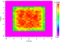
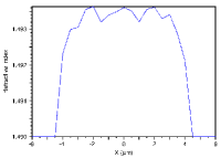
Figure 1: Left: Colour map showing the refractive index profile of a noisy waveguide, Right: Cross-section of the colour map.

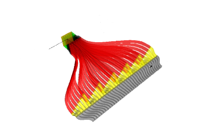
Figure 2: The Photonic Dicer 3D design in the RSoft CAD environment. The colours indicate the 5 different transition planes used.

2.3 Throughput calculation

In order to calculate the total throughput ($T_{\mathrm{tot}}$) of the PD the ratio of the flux in the slit output ($F_{\mathrm{slit}}$) to that of the input field ($F_{\mathrm{ref\star}}$) was taken for each of the science frames. As BeamProp does not take into account any size differences in images, a constant $k$ is used to normalise the input and output spatial sizes of the fields as they were different; this results in

$$\centering\hskip 56.9055pt{T_{\mathrm{tot}}=\frac{F_{\mathrm{slit}}(i)}{F_{\mathrm{ref\star}}(i)\times k},\quad i=\#frames}.\@add@centering$$ (2)

2.4 Dicer Plane Optimisation

The PD was designed in 2013, without the ability to do the full system modelling available using our software suite. This means that there are potential optimisation possibilities that were not taken into account. To investigate this, we use a Monte Carlo simulation routine built into BeamProp to calculate the relative losses for different propagation planes (see Figure 2), changing the size of the PD to the optimal one.

In order for the transitions to have low losses, they should be gradual (Birks et al., 2015). However, as using ULI results in relatively high material and bend losses these transition losses need to be balanced against length.

Simulation results for the optimal device (see Figure 6) show that the optimal PD length is shorter than the constructed one by several mm, leading to greater throughput and a more compact design.

3 Results

3.1 Throughput performance results

Here, the throughput results are presented from the simulation configurations as described in section 2. As stated above, the Soapy AO modes were configured to approximate the on-sky corresponding performance. Consequently, the tip-tilt AO mode was adjusted to perform worse than the open-loop case, in terms of correction, by regulating the seeing/Fried parameter in our simulations (see Table 1). Hence, simulations were performed using our produced Soapy data (phase and amplitude information provided) and real on-sky images acquired in the focal plane at the input of the PD provided by CANARY (Myers et al., 2008). As Canary uses an InGaAs camera only intensity is recorded, therefore for the simulations a flat phase front (all phase = 0) and the square root of the intensity (amplitude) is used.

The results of simulating 12000 frames are shown in Figure 3. For closed-loop operation mode (full AO correction) the transmission of the PD was measured to be 20 $\pm$2 (%). In open-loop operation mode the transmission was measured to be 8 $\pm$2 (%); and for tip-tilt correction results shown to be 9 $\pm$2 (%).

The camera data taken from the on-sky run (real) were also simulated by BeamProp and the results are shown in Table 3. This shows an overestimation of the throughput by a factor of $\sim$2. The reason of this overestimated result is the absence of phase information in the on-sky data fields and as a consequence BeamProp considers zero-phase everywhere.

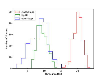
Figure 3: Histogram plot of throughput measurements in the three different AO modes, with each mode containing 12000 simulation results binned by a factor of 60. In order of correction, red shows closed-loop, green tip-tilt correction and blue shows open-loop.

As with Harris et al. (2015) we also investigated the ratio of output power in the slit to input power coupled to the PD, in order to calculate a value of light transmitted through the PD. To do this the ensquared energy (EE) at the input of the PD was calculated and plotted against the corresponding throughput. Figure 4 shows the result of this; as in Harris et al. (2015) we see a positive linear correlation of EE with calculated slit output power. The black line shows where the input EE and output throughput are equal. Some values are close to equal; this is due to evanescent field coupling which is further explained in section 4.3.

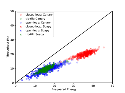
Figure 4: Throughput measurements of the simulated PD slit end versus the amount of light coupled at 321 mas (the square entrance of the device as configured in BeamProp). This is shown for the simulated data of Soapy (bold colour) and on-sky results (transparent) in all three AO operating modes. Note that the number of points are binned by a factor of 60 into 200 points from the 12000, for each AO mode.

Table 3: Fractional throughput results comparing theoretical simulations and on-sky conditions. The incorrect results for real measured input data + BeamProp show a factor of two overestimation because BeamProp assumes zero phase if phase information is not provided; this highlights the importance of having phase information of the input beam in the simulations.

		Data and results
AO mode	On-sky	Soapy	On-sky
		+BeamProp	+BeamProp
closed-loop (%)	20 $\pm$ 2	20 $\pm$ 2	45 $\pm$ 2
tip-tilt (%)	9 $\pm$ 2	9 $\pm$ 2	20 $\pm$ 2
open-loop (%)	11 $\pm$ 2	8 $\pm$ 2	24 $\pm$ 2

For a better understanding of the coupling efficiency EE, the ratio between closed-loop and tip-tilt correction was calculated and plotted versus the device MM entrance input size for averaged Soapy and real data images (Figure 5). This figure illustrates that the EE under closed-loop mode is higher than that of tip-tilt by a factor of $\sim$ 2.8 for real and $\sim$ 2.4 for Soapy data. This factor varies inversely with the spatial size of the sampling as a function of overall throughput.

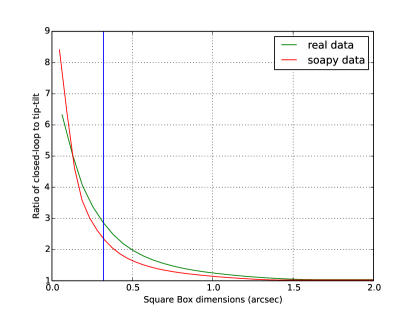
Figure 5: The relation of closed-loop and tip-tilt AO mode ratios of EE as a function of spatial scale (square box centred), plotted for both simulated (Soapy) and on-sky averaged data (real). The PD square entrance size is represented by the blue vertical line.

3.2 Optimisation results

In order to optimise the PD, the average of the real and imaginary parts of the electric field of the frames from a closed-loop dataset by Soapy was chosen. Using this as an input, a Monte Carlo simulation was performed on the PD, optimising each of its transition planes for throughput by scanning for different lengths among the 5 transition planes of the device. The results of this are shown in Figure 6. In this figure, throughput results from simulations with the optimised and unoptimised versions of the PD using all of the three AO modes as an input are plotted against the propagation length of the device. The solid and dashed lines represent the unoptimised and optimised PD, respectively. In this illustration we notice the shorter more efficient version of the PD, as well as the high coupling losses at the entrance input of the device, where the PL section is located. That means the transition can be further improved to be more adiabatic and thus lower in loss.

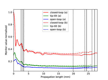
Figure 6: Co-added computed power enclosed inside the 36 waveguides as a function of the propagating length. Vertical solid black lines indicate the 5 transition planes of the device as it was originally built, and vertical dashed black lines represent the optimised locations of the planes. This is shown for the three AO operating modes in three different colours (constant lines for default PD (a) and dashed lines (b) for the optimised version correspondingly). Computed powers are normalised according to the maximum of each AO modes. Averaged frames of all three AO modes were used as an input. Power fluctuations are discussed in section 4.3.

3.3 Modal noise results

To investigate whether our theoretical PD was subject to modal noise, we performed two analyses. The first is similar to a classical modal noise experiment, where the measured barycentre of the slit moves (Rawson et al., 1980; Chen et al., 2006). To do this we chose a single wavelength and examined the stability of the near field image of the slit using our Soapy produced images as an input. The second is a more recently discovered phenomenon, namely periodic variations of throughput as a function of wavelength, due to modal mismatch in the reformatting devices (Spaleniak et al., 2016; Cvetojevic et al., 2017).

To check the stability of the slit, the intensities of output frames from the simulations were averaged. The variation of the mode field diameter (MFD) and its barycentric position were calculated to look for disturbances of the coupled field that are translated to a different speckle pattern at the slit output. Figure 7 presents the analysis results of the PD. In the top panel the averaged slit image (intensity) from BeamProp is illustrated. The middle panel shows the MFD of the slit profile calculated from the Gaussian fit, and the bottom panel depicts the barycentre position of the MFD calculated across the slit. Measurements of the barycentre movement are presented as a portion of one-thousandth of the core diameter ($d$/1000). Results show a mean variation of 1.2 $\upmu$m (10% of the averaged MFD) in the MFD dimension, while the semi amplitude barycentre variation was found to be of the order of $2\times 10^{-4}$ ($d$/1000). It should be noted that the simulations did not include any manufacturing errors in the straightness of the slit. These variations degrade the spectral resolving power and introduce noise and uncertainties in the produced spectra.

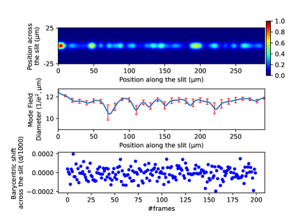
Figure 7: Top panel: Near field averaged image (intensity) of the slit from BeamProp simulations (@1550 nm). Middle panel: MFD of the slit profile including 1$\upsigma$ errors from individual frames. Bottom panel: Near field barycentre shifts across the slit.

Measurements of the throughput were performed in two wavelength regimes; in the first one covering the 1545 - 1555 nm wavelength range with 0.1 nm steps to approximate a typical low resolution spectrum (R $\sim$ 15.500), and in the second one covering the 1554.5 - 1555.5 nm wavelength range with 0.01 nm steps corresponding to a typical high resolution spectrum (R $\sim$155.000). It should be noted that the launch mode profile remained the same in those simulations for all wavelengths, namely a 50 $\upmu$m (MFD @ $\mathrm{1/e^{2}}$) representative of a diffraction-limited input injected into the entrance of the PD. Normalised throughput results are presented in Figure 8, where it can be seen that there is no significant variation of throughput with wavelength, both for high and low resolution simulations.

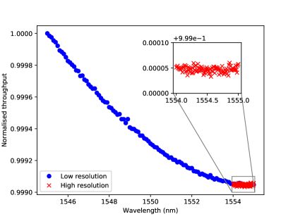
Figure 8: Throughput performance of the PD as a function of wavelength for low spectral resolution scanning with steps of 0.1 nm (R $\sim$ 15.500), and high spectral resolution scanning with steps of 0.01 nm (R $\sim$ 155.000). Inset: High spectral resolution magnified.

4 Discussion

4.1 Adaptive optics performance

In order to match the performance for each AO operation mode, the datasets from Soapy were compared to the corresponding on-sky ones. By comparing the EE within a growing box starting from the centre of averaged data frames as a function of square box spatial dimensions, we matched our simulated to on-sky ones. We found most results converged for the same AO parameters as on-sky, though the mean seeing value of all AO modes used in Soapy was 1.04 arcseconds instead of the 0.7 arcseconds as seen on-sky (see Table 1 & Harris et al. (2015)). This might be caused by various factors, including the unstable atmospheric conditions on-sky, vibrations due to electronics in the telescope and the impact of the wind on the telescope dome and around its components. This raises the question of how best to optimise future simulations and what data to take for future on-sky tests. Future work will involve adding more noise to our simulations to try to better compare our results with on-sky data. It should be noted also that the effect of changing atmospheric conditions was considered in order to represent better the on-sky conditions (see Figure 6 and Table 1 by adjusting the seeing parameter in each AO mode).

4.2 F-ratio calibration

Harris et al. (2015) state that the relative scaling between the calibration and main arms of their experiment configuration had a magnification mismatch. This was caused by errors in focal length calculation due to the extremely short focal length $\sim$ 4.5 mm lenses that imaged the PSF generated by CANARY onto the PD entrance. Our initial tests were performed with their platescale of 7.96 arcseconds/mm (a PD entrance aperture of 405 mas), which led to an underestimation of the on-sky throughput performance. Following further investigation we concluded that a platescale of 6.37 arcseconds/mm (PD entrance aperture of 321 mas) produced a much better fit of the resulting throughput compared to the on-sky results. With the appropriate corrections on magnification, we found that their results fit ours. As their lenses had short focal lengths it is likely that their scaling has large errors, which leads to the mismatch. In future on-sky experiments it would be extremely useful to have accurately characterised optical designs.

4.3 Evanescent field coupling

In Figure 4 we see that the measurements with lower EE (and hence less light into the PD) show a throughput closer to the input EE (a higher device transmission); while when the EE was increased, the fraction of light passing through the PD appears to drop.

To investigate this effect, a test was conducted with three data frames from Soapy, one in closed-loop mode, one in open-loop and one in tip-tilt (full field). As with our other simulations, this was propagated through the PD and the throughput measured. The field outside the PD was then set to zero and the simulation was re-run (cut field). A third simulation was then performed with the field inside the PD set to zero (Cut-inside field) (see Figure 9 (full, cut, cut-inside field)).

To calculate the relative throughput for each simulation per AO mode, we use the following equation

$$\begin{split}T_{\rm{tot}}&=EE_{\rm{b}}\times T_{\rm{b}}+EE_{\rm{c}}\times T_{\rm{c}}\\ 20.53\%&=42.05\%\times 46.28\%+57.94\%\times 1.86\%\\ 9\%&=16.06\%\times 49.07\%+83.94\%\times 1.34\%\\ 11.95\%&=20.4\%\times 50.12\%+79.6\%\times 2.17\%\end{split}$$ (3)

Where $EE_{\rm{a,b,c}}$ the percentage of the light in the partial simulation ($EE_{\rm{a}}=EE_{\rm{b}}+EE_{\rm{c}}=100\%$), and $T_{\rm{b,c}}$ the throughput in the partial simulation.

Table 4: Evanescent field contribution results (See section 4.3)

	Full field	Cut field	Cut-inside field
AO mode	(Throughput)	$(EE_{\rm{b}}\times T_{\rm{b}}$)	$(EE_{\rm{c}}\times T_{\rm{c}}$)
closed-loop (%)	20.53	42.05 $\times$ 46.28	57.94 $\times$ 1.86
tip-tilt (%)	9	16.06 $\times$ 49.07	83.94 $\times$ 1.34
open-loop (%)	11.95	20.4 $\times$ 50.12	79.6$\times$ 2.17

The results from this are shown in Table 4. This result shows that the light coupled into the PD was not coupled entirely at the entrance to the PD. We can explain this as being due to the small refractive index difference between core and cladding ($\mathrm{\Delta\approx 1.76\times 10^{-3}}$). This gives the PD a large evanescent field, which couples light into the waveguides.

We looked into this further, by examining the partial power monitors in RSoft as the light propagated along the waveguides. Figure 6 shows the normalised power within the waveguides. As expected, this drops as the light propagates through the PD. However in the second to last section we see the power increasing slightly. This is due to the power monitors in RSoft not taking the evanescent field of the waveguides into account. As the waveguides in the second to last section are brought together, the evanescent field from each one is coupled into the adjacent waveguide, which means the evanescent fields overlap, increasing the measured power in the PD.

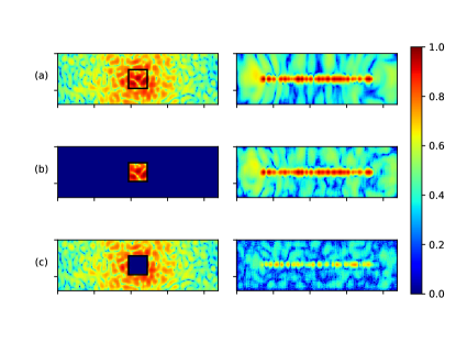
Figure 9: (a-c) Colour map images (logarithm of intensities) of the Soapy closed AO mode input data at the left together with the corresponding reformatted output of the PD at the right, for 3 different EE coupled to device spatial simulation domain, (a - full field) and (b - cut field) 42.05 % of the full frame, (c - cut-inside field) 57.94 % of the full frame. The simulated spatial domain for each of the 6 frames is 438$\times$138 $\upmu$m.

To summarise, our findings indicate that up to 2% of the light within the slit output originates from evanescent field coupling. Thus, a slit mask should be used in front of the PD entrance if the evanescent field is undesired depending on the scientific goals.

4.4 Modal noise

As we can see from the bottom panel in Figure 7 the modal pattern in the slit is not straight and has some limited residual movement even though the slit was configured to be straight. This, as with modal noise, will limit the spectral resolving power of the spectrograph, though not to the same extent as with the modal noise in conventional fibres (Chen et al., 2006). In order to prove that statement two experiments were performed to justify our hypothesis. Firstly, following the procedure as described in section 3.3 the variation of the MFD and its barycentric position were calculated for a device identical to the PD, though at the output level of the slit the waveguides were separated and not touching each other. Secondly, the same method was applied to a common circular MM fibre 50 $\upmu$m in diameter with a NA = 0.22 and refractive index of the core equal to 1.45. Results suggest that for the separated version of the PD, barycentric movement is 50% more stable than the original version of the PD (semi amplitude variation $10^{-4}$ ($d$/1000), see Figure 10), while for the MM fibre case the barycentre movement of the average of the speckles that were calculated, is three orders larger than the PD (semi amplitude variation $2\times 10^{-2}$ ($d$/1000), see Figure 11) and qualitatively similar to results in the literature (e.g. Feger et al. (2012)).

It should be cautioned that, as noted in Spaleniak et al. (2016) any imperfections in the manufacture of the slit will result in modal noise due to movement of the barycentre of the MFD. Following our results above, we would suggest (as already pointed out in the aforementioned paper) separated slit cores, to allow reduction of this modal noise.

We also see no variation in throughput with wavelength for the PD, as seen with similar devices and wavelength regimes (e.g. (Spaleniak et al., 2016; Cvetojevic et al., 2017)). This suggests our device is free of noise caused by modal mismatch between components (e.g. the mismatch between a MM fibre and PL in Cvetojevic et al. (2017)).

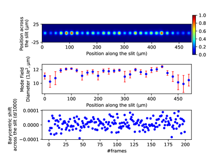
Figure 10: Top panel: Near field averaged image (intensity) of the separated slit from BeamProp simulations. Middle panel: MFD of the slit profile including 1$\upsigma$ errors from individual frames. Bottom panel: Measurements of barycentre movement across the slit from individual frames.

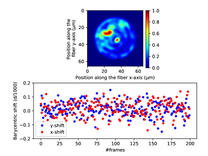
Figure 11: Top panel: Typical near field image of the 50 $\upmu$m MM fibre output from BeamProp simulations. Bottom panel: Measurements of barycentre movement along the fibre y-axis (blue) and x-axis (red) from individual frames.

5 Conclusions

We have conducted a theoretical study concerning the performance of an existing astrophotonic component, the photonic dicer. We make use of Soapy, a Monte Carlo AO simulation program to model the atmosphere and its impact on the performance of the device, and BeamProp by RSoft, a finite-difference beam propagation solver to simulate the device itself. The simulated AO corrected PSFs were used as an input to our replicated PD in RSoft.

Our results matched the on-sky results well. Showing a simulated throughput of 20 $\pm$ 2% in closed-loop (compared to the same value on-sky), 9 $\pm$ 2% in tip-tilt (compared to the same value on-sky) and 8 $\pm$ 2% in open-loop (compared to 11 $\pm$ 2% for on-sky). The slight variation is likely due to changing atmospheric seeing during the course of the observations, which were only partially reproduced in the simulation.

We also investigated the effect of modal noise on the PD. We showed that although it is not completely modal noise free it should show a reduction of three orders of magnitude as compared to a standard MM fibre. This can also be improved by separating the output slit, as suggested in Spaleniak et al. (2016).

Further simulations were used to optimise the device and showed a throughput improvement of 6.4%. This shows the importance of fully simulating such devices, in particular with atmospheric effects.

Our simulations also revealed an error in magnification at the input of the photonic dicer reported in Harris et al. (2015). A value of 7.96 arcseconds/mm was reported for the plate scale while our investigation resulted in a plate scale of 6.37 arcseconds/mm. Optimising this will be important in future work for both the devices and also the adaptive optics performance.

Our results suggest that detailed simulations are a valuable tool for the design of new components for astronomy with the aim of enabling more precise measurements, easier calibration of the acquired data, and more compact instruments for future telescopes. Simulations like ours can be used to estimate the on-sky performance in non ideal observing conditions.

Aims for future work include further optimisation for better coupling to the telescope point spread function by repositioning of the photonic dicer entrance wave-guide positions and improvement of the transmission of the device by a better manufacturing process. Additionally, there is high potential for more advanced photonic instrument concepts such as an integrated spatial reformatter feeding an arrayed waveguide grating (AWG) (Stoll et al., 2017; Cvetojevic et al., 2017).

References

- Agapito et al. (2014) Agapito G., Arcidiacono C., Quirós-Pacheco F., Esposito S., 2014, Experimental Astronomy, 37, 503
- Allington-Smith et al. (2002) Allington-Smith J., et al., 2002, PASP, 114, 892
- Birks et al. (2015) Birks T. A., Gris-Sánchez I., Yerolatsitis S., Leon-Saval S. G., Thomson R. R., 2015, Adv. Opt. Photon., 7, 107
- Bland-Hawthorn & Horton (2006) Bland-Hawthorn J., Horton A., 2006, Proc. SPIE, 6269, 62690N
- Bland-Hawthorn et al. (2010) Bland-Hawthorn J., et al., 2010, Proc. SPIE, 7735, 77350N
- Bouchy et al. (2013) Bouchy F., Díaz R. F., Hébrard G., Arnold L., Boisse I., Delfosse X., Perruchot S., Santerne A., 2013, A&A, 549, A49
- Chen et al. (2006) Chen C.-H., Reynolds R. O., Kost A., 2006, Appl. Opt., 45, 519
- Coudé du Foresto (1994) Coudé du Foresto V., 1994, IAU Symposium, 158, 261
- Crepp (2014) Crepp J. R., 2014, Science, 346, 809
- Cunningham (2009) Cunningham C., 2009, Nature Photonics, 3, 239
- Cvetojevic et al. (2009) Cvetojevic N., Lawrence J. S., Ellis S. C., Bland-Hawthorn J., Haynes R., Horton A., 2009, Opt. Express, 17, 18643
- Cvetojevic et al. (2012) Cvetojevic N., Jovanovic N., Lawrence J., Withford M., Bland-Hawthorn J., 2012, Opt. Express, 20, 2062
- Cvetojevic et al. (2017) Cvetojevic N., et al., 2017, Opt. Express, 25, 25546
- Dekany et al. (2013) Dekany R., et al., 2013, ApJ, 776, 130
- Feger et al. (2012) Feger T., Brucalassi A., Grupp F. U., Lang-Bardl F., Holzwarth R., Hopp U., Bender R., 2012, Proc. SPIE, 8446, 844692
- Halverson et al. (2015) Halverson S., Roy A., Mahadevan S., Schwab C., 2015, ApJ, 814, L22
- Harris & Allington-Smith (2013) Harris R. J., Allington-Smith J. R., 2013, MNRAS, 428, 3139
- Harris et al. (2015) Harris R. J., et al., 2015, MNRAS, 450, 428
- Hook et al. (2004) Hook I. M., Jørgensen I., Allington-Smith J. R., Davies R. L., Metcalfe N., Murowinski R. G., Crampton D., 2004, PASP, 116, 425
- Hunter (2007) Hunter J. D., 2007, Computing In Science & Engineering, 9, 90
- Iuzzolino et al. (2014) Iuzzolino M., Tozzi A., Sanna N., Zangrilli L., Oliva E., 2014, Proc. SPIE, 9147, 914766
- Jovanovic et al. (2015) Jovanovic N., et al., 2015, PASP, 127, 890
- Jovanovic et al. (2016) Jovanovic N., Schwab C., Cvetojevic N., Guyon O., Martinache F., 2016, PASP, 128, 121001
- Lemke et al. (2011) Lemke U., Corbett J., Allington-Smith J., Murray G., 2011, MNRAS, 417, 689
- Leon-Saval et al. (2005) Leon-Saval S. G., Birks T. A., Bland-Hawthorn J., Englund M., 2005, in Optical Fiber Communication Conference and Exposition and The National Fiber Optic Engineers Conference. Optical Society of America, p. PDP25, http://www.osapublishing.org/abstract.cfm?URI=OFC-2005-PDP25
- Leon-Saval et al. (2012) Leon-Saval S. G., Betters C. H., Bland-Hawthorn J., 2012, Proc. SPIE, 8450, 84501K
- Leon-Saval et al. (2013) Leon-Saval S. G., Argyros A., Bland-Hawthorn J., 2013, Nanophotonics, 2, 429
- MacLachlan et al. (2014) MacLachlan D. G., Harris R., Choudhury D., Arriola A., Brown G., Allington-Smith J., Thomson R. R., 2014, Proc. SPIE, 9151, 91511W
- MacLachlan et al. (2017) MacLachlan D. G., et al., 2017, MNRAS, 464, 4950
- Macintosh et al. (2014) Macintosh B., et al., 2014, Proceedings of the National Academy of Science, 111, 12661
- Mayor et al. (2003) Mayor M., et al., 2003, The Messenger, 114, 20
- McCoy et al. (2012) McCoy K. S., Ramsey L., Mahadevan S., Halverson S., Redman S. L., 2012, Proc. SPIE, 8446, 84468J
- Mueller et al. (2014) Mueller M., et al., 2014, Proc. SPIE, 9147, 91479A
- Myers et al. (2008) Myers R. M., et al., 2008, Proc. SPIE, 7015, 70150E
- Nasu et al. (2005) Nasu Y., Kohtoku M., Hibino Y., 2005, Opt. Lett., 30, 723
- Noguchi et al. (2002) Noguchi K., et al., 2002, Publications of the Astronomical Society of Japan, 54, 855
- Perruchot et al. (2011) Perruchot S., et al., 2011, Proc. SPIE, 8151, 815115
- Probst et al. (2015) Probst R. A., et al., 2015, New Journal of Physics, 17, 023048
- Quirrenbach et al. (2016) Quirrenbach A., et al., 2016, Proc. SPIE, 9908, 990812
- Rawson et al. (1980) Rawson E. G., Goodman J. W., Norton R. E., 1980, J. Opt. Soc. Am., 70, 968
- Reeves (2016) Reeves A., 2016, Proc. SPIE, 9909, 99097F
- Schwab et al. (2014) Schwab C., Leon-Saval S. G., Betters C. H., Bland-Hawthorn J., Mahadevan S., 2014, IAU Symposium, 293, 403
- Spaleniak et al. (2013) Spaleniak I., Jovanovic N., Gross S., Ireland M. J., Lawrence J. S., Withford M. J., 2013, Optics Express, 21, 27197
- Spaleniak et al. (2016) Spaleniak I., et al., 2016, Proc. SPIE, 9912, 991228
- Stoll et al. (2017) Stoll A., Zhang Z., Haynes R., Roth M., 2017, Photonics, 4
- (46) Synopsys, RSoft Photonic System Design Suite Version 2017.03, https://optics.synopsys.com/rsoft/
- Thomson et al. (2011) Thomson R., Birks T., Leon-Saval S., Kar A., Bland-Hawthorn J., 2011, Optics Express, 19, 5698
- Tollestrup et al. (2012) Tollestrup E. V., Pazder J., Barrick G., Martioli E., Schiavon R., Anthony A., Halman M., Veillet C., 2012, Proc. SPIE, 8446, 84462A
- Van der walt et al. (2011) Van der walt S., Colbert S. C., Gaël V., 2011, Computing in Science & Engineering, 13, 22
- Vogt et al. (1994) Vogt S. S., et al., 1994, Proc. SPIE, 2198, 362
- Weitzel et al. (1996) Weitzel L., Krabbe A., Kroker H., Thatte N., Tacconi-Garman L. E., Cameron M., Genzel R., 1996, A&AS, 119, 531
- Yerolatsitis et al. (2017) Yerolatsitis S., Harrington K., Birks T. A., 2017, Optics Express, 25, 18713
- Zerbi et al. (2014) Zerbi F. M., et al., 2014, Proc. SPIE, 9147, 914723