Distributed Big-Data Optimization
via Block-Iterative Convexification and Averaging

Abstract

In this paper, we study distributed big-data nonconvex optimization in multi-agent networks. We consider the (constrained) minimization of the sum of a smooth (possibly) nonconvex function, i.e., the agents’ sum-utility, plus a convex (possibly) nonsmooth regularizer. Our interest is in big-data problems wherein there is a large number of variables to optimize. If treated by means of standard distributed optimization algorithms, these large-scale problems may be intractable, due to the prohibitive local computation and communication burden at each node. We propose a novel distributed solution method whereby at each iteration agents optimize and then communicate (in an uncoordinated fashion) only a subset of their decision variables. To deal with non-convexity of the cost function, the novel scheme hinges on Successive Convex Approximation (SCA) techniques coupled with i) a tracking mechanism instrumental to locally estimate gradient averages; and ii) a novel block-wise consensus-based protocol to perform local block-averaging operations and gradient tacking. Asymptotic convergence to stationary solutions of the nonconvex problem is established. Finally, numerical results show the effectiveness of the proposed algorithm and highlight how the block dimension impacts on the communication overhead and practical convergence speed.

I Introduction

In many modern control, estimation, and learning applications, optimization problems with a very-high dimensional decision variable arise. These problems are often referred to as big-data and call for the development of new algorithms. A lot of attention has been devoted in recent years to devise parallel, possibly asynchronous, algorithms to solve problems of this sort on shared-memory systems. Distributed optimization has also received significant attention, since it provides methods to solve cooperatively networked optimization problems by exchanging messages only with neighbors and without resorting to any shared memory or centralized coordination.

In this paper, we consider distributed big-data optimization, that is, big-data problems that must be solved by a network of agents in a distributed way. We are not aware of any work in the literature that can address the challenges of big-data optimization over networks. We organize the relevant literature in two groups, namely: (i) centralized and parallel methods for big-data optimization, and (ii) primal distributed methods for multi-agent optimization.

A coordinate-descent method for huge-scale smooth optimization problems has been introduced in [1], and then extended in [2, 3, 4] to deal with (convex) composite objective functions in a parallel fashion. A parallel algorithm based on Successive Convex Approximation (SCA) has been proposed in [5] to cope with non-convex objective functions. An asynchronous extension has been proposed in [6]. In [7] a parallel stochastic-gradient algorithm has been studied wherein each processor randomly chooses a component of the sum-utility function and updates only a block (chosen uniformly at random) of the entire decision variable. Finally, an asynchronous parallel mini-batch algorithm for stochastic optimization has been proposed in [8]. These algorithms, however, are not implementable efficiently in a distributed network setting, because either they assume that all agents know the whole sum-utility or that, at each iteration, each agent has access to the other agents’ variables.

In the last years, distributed multi-agent optimization has received significant attention. Here, we refer only to distributed primal methods, which are more closely related to the approach proposed in this paper. In [9], a coordinate descent method to solve linearly constrained problems over undirected networks has been proposed. In [10] a broadcast-based algorithm over time-varying digraphs has been studied, and its extension to distributed online optimization has been considered in [11]. In [12] a distributed algorithm for convex optimization over time-varying networks in the presence of constraints and uncertainty using a proximal minimization approach has been proposed. A distributed algorithm, termed NEXT, combining SCA techniques with a novel gradient tracking mechanism instrumental to estimate locally the average of the agents’ gradients, has been proposed in [13, 14] to solve nonconvex constrained optimization problems over time-varying networks. The scheme has been extended in  [15, 16] to deal with directed (time-varying) graphs. More recently in [17] and [18], special instances of the two aforementioned algorithms have been shown to enjoy geometric convergence rate when applied to unconstrained smooth (strongly) convex problems. A Newton-Raphson consensus strategy has been introduced in [19] to solve unconstrained, convex optimization problems leveraging asynchronous, symmetric gossip communications. The same technique has been extended to design an algorithm for directed, asynchronous, and lossy communications networks in [20]. None of these schemes can efficiently deal with big-data problems. In fact, when it comes to big-data problems, local computation and communication requirements need to be explicitly taken into account in the algorithmic design. Specifically, (i) local optimization steps on the entire decision variable cannot be performed, because they would be too computationally demanding; and (ii) communicating, at each iteration, the entire vector of variables of the agents would incur in an unaffordable communication overhead.

First attempts to distributed big-data optimization are [21, 22] for a structured, partitioned, optimization problem, and [23] by means of a partial stochastic gradient for strongly convex smooth problems. These schemes however are not applicable to multi-agent problems wherein the agents’ functions are not (partially) separable.

In this paper, we propose the first distributed algorithm for (possibly nonconvex) big-data optimization problems over networks, modeled as digraphs. To cope with the issues posed by big-data problems, in the proposed scheme, agents maintain a local estimate of the common decision variables but, at every iteration, they update and communicate only one block. Blocks are selected in an uncoordinated fashion among the agents by means of an “essentially cyclic rule” guaranteeing that all blocks are persistently updated. Specifically, each agent minimizes a strongly-convex local approximation of the nonconvex sum-utility function with respect to the selected block variable only. Inspired by the SONATA algorithm [16], the surrogate is based on the agent local cost-function and a local gradient estimate (of the smooth global-cost portion). The optimization step is combined with a block-wise consensus step, tracking the network average gradient and guaranteeing the asymptotic agreement of the local solution estimates to a common stationary solution of the nonconvex problem.

The paper is organized as follows. In Section II, we present the problem set-up and recall some preliminaries. In Section III, we first introduce the new block-wise consensus protocol, and then formally present our novel distributed big-data optimization algorithm along with its convergence properties. Finally, in Section IV, we show a numerical example to test our algorithm.

II Distributed Big-Data Optimization:
Set-up and Preliminaries

In this section, we introduce the big-data optimization set-up and recall two distributed optimization algorithms inspiring the one we propose in this paper.

II-A Distributed Big-Data Optimization Set-up

We consider a multi-agent system composed of $N$ agents, aiming at solving cooperatively the following (possibly) nonconvex, nonsmooth, large-scale optimization problem

$$\begin{split}\min_{\mathbf{x}}\,\,\,\,\,\>&\>U(\mathbf{x})\triangleq\sum_{i=1}^{N}f_{i}(\mathbf{x})+\sum_{\ell=1}^{B}g_{\ell}(\mathbf{x}_{\ell})\\ \text{subj.\ to}\>&\>\mathbf{x}_{\ell}\in\mathcal{K}_{\ell},\quad\ell\in\{1,\ldots,B\},\end{split}$$ (P)

where $\mathbf{x}$ is the vector of optimization variables, partitioned in $B$ blocks

$$\mathbf{x}\triangleq\begin{bmatrix}\mathbf{x}_{1}\\[-3.99994pt] \vdots\\[-3.99994pt] \mathbf{x}_{B}\end{bmatrix},$$

with each $\mathbf{x}_{\ell}\in^{d}$, $\ell\in\{1,\ldots,B\}$; $f_{i}:^{dB}\rightarrow$ is the cost function of agent $i$, assumed to be smooth but (possibly) nonconvex; $g_{\ell}:^{d}\rightarrow$, $\ell\in\{1,\ldots,B\}$, is a convex (possibly nonsmooth) function; and $\cal K_{\ell}$, $\ell\in\{1,\ldots,B\}$, is a closed convex set. Usually the nonsmooth term in (P) is used to promote some extra structure in the solution, such as (group) sparsity. In the following, we will denote by $\mathcal{K}\triangleq\mathcal{K}_{1}\times\cdots\times\mathcal{K}_{B}$ the feasible set of (P). We study problem (P) under the following assumptions.

Assumption II.1 (On the optimization problem)

1. Each $\mathcal{K}_{\ell}\neq\emptyset$ is closed and convex;

2. Each $f_{i}:\mathbb{R}^{dB}\rightarrow\mathbb{R}$ is $C^{1}$ on (an open set containing) $\mathcal{K}$;

3. Each $\nabla f_{i}$ is $L_{i}$-Lipschitz continuous and bounded on $\mathcal{K}$;

4. Each $g_{\ell}:\mathbb{R}^{d}\rightarrow\mathbb{R}$ is convex (possibly nonsmooth) on (an open set containing) $\mathcal{K}$, with bounded subgradients over $\mathcal{K}$;

5. $U$ is coercive on $\mathcal{K}$, i.e., $\operatornamewithlimits{lim\vphantom{p}}_{\mathbf{x}\in\mathcal{K},\|\mathbf{x}\|\to\infty}U(\mathbf{x})=\infty$. $\square$

The above assumptions are quite standard and satisfied by many practical problems; see, e.g. [5]. Here, we only remark that we do not assume any convexity of $f_{i}$. In the following, we also make the blanket assumption that each agent $i$ knows only its own cost function $f_{i}$ (the regularizers $g_{\ell}$ and the feasible set $\cal K$) but not the other agents’ functions.

On the communication network: The communication network of the agents is modeled as a fixed, directed graph $\mathcal{G}=(\{1,\ldots,N\},\mathcal{E})$, where $\mathcal{E}\subseteq\{1,\ldots,N\}\times\{1,\ldots,N\}$ is the set of edges. The edge $(i,j)$ models the fact that agent $i$ can send a message to agent $j$. We denote by $\mathcal{N}_{i}$ the set of in-neighbors of node $i$ in the fixed graph $\mathcal{G}$ including itself, i.e., $\mathcal{N}_{i}\triangleq\left\{j\in\{1,\ldots,N\}\mid(j,i)\in\mathcal{E}\right\}{\cup\{i\}}$. We make the following assumption on the graph connectivity.

Assumption II.2

The graph $\mathcal{G}$ is strongly connected.  $\square$

Algorithmic Desiderata: Our goal is to solve problem (P) in a distributed fashion, leveraging local communications among neighboring agents. As a major departure from current literature on distributed optimization, here we focus on big-data instances of problem (P) wherein the vector of variables $\mathbf{x}$ is composed of a huge number of components ($B$ is very large). In such problems, minimizing the sum-utility with respect to the whole $\mathbf{x}$, or even computing the gradient or evaluating the value of a single function $f_{i}$, can require substantial computational efforts. Moreover, exchanging an estimate of the entire local decision variable $\mathbf{x}$ over the network (like current distributed schemes do) is not efficient or even feasible, due to the excessive communication overhead. We design next the first scheme able to deal with such challenges. To this end, we first review two existing distributed algorithms for nonconvex optimization that will act as building blocks for our novel algorithm.

II-B NEXT and SONATA: A Quick Overview

In [13, 14] a distributed algorithm, termed NEXT, is proposed to solve nonconvex optimization problems in the form (P). The algorithm is based on an iterative two-step procedure whereby all the agents first update their local estimate $\mathbf{x}_{(i)}$ of the optimization variable $\mathbf{x}$ by solving a suitably chosen convexification of (P), and then communicate with their neighbors to asymptotically force an agreement among the local variables while converging to a stationary solution of (P). The strongly convex approximation of the original noncovex function has the following form: The nonconvex cost function $f_{i}$ is replaced by a suitable strongly convex surrogate function $\tilde{f}_{i}$ (see [5]) whereas the sum of the unknown functions of the other agents $\sum_{j\neq i}f_{j}$ is approximated by a linear term whose coefficients track the gradient of $\sum_{j\neq i}f_{j}$. More formally, given the current iterate $\mathbf{x}_{(i)}^{t}$, the optimization step reads:

$$\widetilde{\mathbf{x}}_{(i)}^{t} =\mathop{\rm argmin}_{\mathbf{x}\in\mathcal{K}}\tilde{f}_{i}(\mathbf{x};\mathbf{x}_{(i)}^{t})+(\mathbf{x}-\mathbf{x}_{(i)}^{t})^{\top}\widetilde{\boldsymbol{\pi}}_{(i)}^{t}+g(\mathbf{x}),$$

$$\mathbf{v}_{(i)}^{t} =\mathbf{x}_{(i)}^{t}+\gamma^{t}(\widetilde{\mathbf{x}}_{(i)}^{t}-\mathbf{x}_{(i)}^{t}),$$

where $\widetilde{\boldsymbol{\pi}}_{(i)}^{t}$ is a local estimate of $\sum_{j\neq i}\nabla f_{j}(\mathbf{x}_{(i)}^{t})$ (that needs to be properly updated); $g(\mathbf{x})\triangleq\sum_{\ell=1}^{B}g_{\ell}(\mathbf{x}_{\ell})$; and $\gamma^{t}$ is the step-size. Given $\widetilde{\mathbf{x}}_{(i)}^{t}$ and $\mathbf{x}_{(i)}^{t}$, the local variable is updated from $\mathbf{x}_{(i)}^{t}$ along the direction $\widetilde{\mathbf{x}}_{(i)}^{t}-\mathbf{x}_{(i)}^{t}$ using the step-size value $\gamma^{t}$. The resulting $\mathbf{v}_{(i)}^{t}$ will then be averaged with the neighboring counterparts to enforce a consensus.

The second step of NEXT, consists in communicating with the neighbors in order to update the local decision variables as well as the gradient estimates $\widetilde{\boldsymbol{\pi}}_{(i)}^{t}$. Formally, we have the following two consensus-based updates:

$$\mathbf{x}_{(i)}^{t+1} =\sum_{j\in\mathcal{N}_{i}}a_{ij}\mathbf{v}_{(j)}^{t},$$

$$\mathbf{y}_{(i)}^{t+1} =\sum_{j\in\mathcal{N}_{i}}a_{ij}\mathbf{y}_{(j)}^{t}+\nabla f_{i}(\mathbf{x}_{(i)}^{t+1})-\nabla f_{i}(\mathbf{x}_{(i)}^{t}),$$

$$\widetilde{\boldsymbol{\pi}}_{(i)}^{t+1} =N\cdot\mathbf{y}_{(i)}^{t}\!-\!\nabla f_{i}(\mathbf{x}_{(i)}^{t+1}),$$

where $\mathbf{y}_{(i)}^{t}$ is an auxiliary local variable (exchanged among neighbors) instrumental to update $\widetilde{\boldsymbol{\pi}}_{(i)}^{t}$; and $\mathbf{A}\triangleq[a_{ij}]_{i,j=1}^{N}$ is a doubly-stochastic matrix that matches the communication graph $\mathcal{G}$: $a_{ij}>0$, if $j\in\mathcal{N}_{i}$; and $a_{ij}=0$ otherwise.

Note that NEXT requires the weight matrices $\mathbf{A}$ to be doubly-stochastic, which limits the applicability of the algorithm to directed graphs. SONATA, proposed in [15, 16], overcomes this limitation by replacing the plain consensus scheme of NEXT with a push-sum-like mechanism, which recovers dynamic average consensus of the local decision variable $\mathbf{x}_{(i)}^{t}$ and gradient estimates $\mathbf{y}_{(i)}^{t}$ by using only column stochastic weight matrices. Introducing an auxiliary local variable $\phi_{(i)}^{t}$ at each agent’s side, the consensus protocol of SONATA reads

$$\phi_{(i)}^{t+1} =\sum_{j\in\mathcal{N}_{i}}a_{ij}\phi_{(j)}^{t},$$

$$\mathbf{x}_{(i)}^{t+1} =\frac{1}{\phi_{(i)}^{t+1}}\sum_{j\in\mathcal{N}_{i}}a_{ij}\phi_{(j)}^{t}\mathbf{v}_{(j)}^{t},$$

$$\mathbf{y}_{(i)}^{t+1} =\frac{1}{\phi_{(i)}^{t+1}}\!\left(\sum_{j\in\mathcal{N}_{i}}\!a_{ij}\,\phi_{(j)}^{t}\mathbf{y}_{(j)}^{t}+\nabla f_{i}(\mathbf{x}_{(i)}^{t+1})-\nabla f_{i}(\mathbf{x}_{(i)}^{t})\!\right)\!,$$

$$\widetilde{\boldsymbol{\pi}}_{(i)}^{t+1} =N\cdot\mathbf{y}_{(i)}^{t}-\nabla f_{i}(\mathbf{x}_{(i)}^{t+1}),$$

where now $\mathbf{A}\triangleq[a_{ij}]_{i,j=1}^{N}$ is only column stochastic (still matching the graph $\mathcal{G}$).

III Block-SONATA Distributed Algorithm

In this section we introduce our distributed big-data optimization algorithm. Differently from current distributed methods, our algorithm performs block-wise updates and communications. A building block of the proposed scheme is a block-wise consensus protocol of independent interest, which is introduced next (cf. Sec. III-A). Then, we will be ready to describe our new algorithm (cf. Sec. III-B).

III-A Block-wise Consensus

We propose a push-sum-like scheme that acts at the level of each block $\ell\in\{1,\ldots,B\}$. Specifically, consider a system of $N$ agents, whose communication network is modeled as a digraph $\cal G$ satisfying Assumption II.2; and let the agents aim at agreeing on the (weighted) average value of their initial states $\mathbf{x}_{(i)}^{0}$, $i\in\{1,\ldots,N\}$. While at each iteration $t$ agents can update their entire vector $\mathbf{x}_{(i)}^{t}$, they can however send to their neighbors only one block; let denote by $\mathbf{x}_{(i,\ell_{i}^{t})}$ the block $\ell_{i}^{t}$ that, at time $t$, agent $i$ selects (according to a suitably chosen rule) and sends to its neighbors, with $\ell_{i}^{t}\in\{1,\ldots,B\}$. Thus, at each iteration, agent $i$ runs a consensus protocol on the $\ell$-th block by using only information received from in-neighbors that have sent block $\ell$ at time $t$ (if any). A natural way to model this protocol is to introduce a block-dependent neighbor set, defined as

$$\mathcal{N}_{i,\ell}^{t}\triangleq\{j\in\mathcal{N}_{i}\mid\ell_{j}^{t}=\ell\}\cup\{i\}\subseteq\mathcal{N}_{i},$$

which includes, besides agent $i$, only the in-neighbors of agent $i$ in $\mathcal{G}$ that have sent block $\ell$ at time $t$. Consistently, we denote by $\mathcal{G}_{\ell}^{t}\triangleq(\{1,\ldots,N\},\mathcal{E}_{\ell}^{t})$ the time-varying subgraph of $\mathcal{G}$ associated to block $\ell$ at iteration $t$. Its edge set is

$$\mathcal{E}_{\ell}^{t}\triangleq\{(j,i)\in\mathcal{E}\mid j\in\mathcal{N}_{i,\ell}^{t},i\in\{1,\ldots,N\}\}.$$

Following the idea of consensus protocols over time-varying digraphs, we introduce a weight matrix $\mathbf{A}_{\ell}^{t}\triangleq[a_{ij\ell}^{t}]_{i,j=1}^{N}$ matching $\mathcal{G}_{\ell}^{t}$, such that $a_{ij\ell}^{t}\in[\theta,1]$, for some $\theta\in(0,1)$, if $j\in\mathcal{N}_{i,\ell}^{t}$; and $a_{ij\ell}^{t}=0$ otherwise. Using $\mathbf{A}_{\ell}^{t}$, we can rewrite the consensus scheme of SONATA block-wise as

$$\begin{split}\phi_{(i,\ell)}^{t+1}&=\sum_{j\in\mathcal{N}_{i}}a_{ij\ell}^{t}\phi_{(j,\ell)}^{t},\hskip 54.06006pt\ell\in\{1,\ldots,B\},\\ \mathbf{x}_{(i,\ell)}^{t+1}&=\dfrac{1}{\phi_{(i,\ell)}^{t+1}}\sum_{j\in\mathcal{N}_{i}}a_{ij\ell}^{t}\phi_{(j,\ell)}^{t}\,\mathbf{x}_{(j,\ell)}^{t},\hskip 5.69046pt\ell\in\{1,\ldots,B\},\end{split}$$ (1)

where $\phi_{(i,\ell)}^{0}$ and $\mathbf{x}_{(i,\ell)}^{0}$ are given, for all $i\in\{1,\ldots,N\}$.

We study now under which conditions the block consensus protocol (1) reaches an asymptotic agreement.

For push-sum-like algorithms (as the one just stated) to achieve asymptotic consensus, the following standard assumption is needed.

Assumption III.1

For all $\ell\in\{1,\ldots,B\}$ and $t\geq 0$, the matrix $\mathbf{A}_{\ell}^{t}$ is column stochastic, that is, $\mathbf{1}^{\top}\mathbf{A}_{\ell}^{t}=\mathbf{1}^{\top}$. $\square$

We show next how nodes can locally build a matrix $\mathbf{A}_{\ell}^{t}$ satisfying Assumption III.1 for each time-varying, directed graph $\mathcal{G}_{\ell}^{t}$. Since in our distributed optimization algorithm we work with a static, strongly connected digraph $\mathcal{G}$ (cf. Assumption II.2), we assume that a column stochastic matrix $\tilde{\mathbf{A}}$ that matches $\mathcal{G}$ is available, i.e., $\tilde{a}_{ij}>0$ if $(j,i)\in\mathcal{E}$ and $\tilde{a}_{ij}=0$ otherwise, and $\mathbf{1}^{\top}\tilde{\mathbf{A}}=\mathbf{1}^{\top}\tilde{\mathbf{A}}$.

To show how $\mathbf{A}_{\ell}^{t}$ can be constructed in a distributed way, we start observing that at iteration $t$, an agent $j$ either sends a block $\ell$ to all its out-neighbors in $\mathcal{G}$, $\ell=\ell_{j}^{t}$, or to none, $\ell\neq\ell_{j}^{t}$. Thus, let us concentrate on the $j$-th column $\mathbf{A}_{\ell}^{t}(:,j)$ of $\mathbf{A}_{\ell}^{t}$. If agent $j$ does not send block $\ell$ at iteration $t$, $\ell\neq\ell_{j}^{t}$, then all elements of $\mathbf{A}_{\ell}^{t}(:,j)$ will be zero except $a_{jj\ell}^{t}$. Thus, to be the $j$-th column stochastic, it must be $\mathbf{1}^{\top}\mathbf{A}_{\ell}^{t}(:,j)=a_{jj\ell}^{t}=1$ (i.e., $\mathbf{A}_{\ell}^{t}(:,j)$ is the $j$-th vector of the canonical basis). Viceversa, if $j$ sends block $\ell$, all its out-neighbors in $\mathcal{G}$ will receive it and, thus, column $\mathbf{A}_{\ell}^{t}(:,j)$ has the same nonzero entries as column $\tilde{\mathbf{A}}(:,j)$ of $\tilde{\mathbf{A}}$. Since $\tilde{\mathbf{A}}$ is column stochastic, the same entries can be chosen, that is, $\mathbf{A}_{\ell}^{t}(:,j)=\tilde{\mathbf{A}}(:j)$. This rule can be stated from the point of view of each agent $i$ and its in-neighbors, thus showing that each agent can locally construct its own weights. For each $i\in\{1,\ldots,N\}$ and $\ell\in\{1,\ldots,B\}$, weights $a_{ij\ell}^{t}$ can be defined as

$$a_{ij\ell}^{t}\triangleq\begin{cases}\tilde{a}_{ij},&\text{if }j\in\mathcal{N}_{i}\text{ and }\ell=\ell_{j}^{t},\\ 1,&\text{if }j=i\text{ and }\ell\neq\ell_{j}^{t},\\ 0,&\textnormal{otherwise}.\end{cases}$$ (2)

Besides imposing $\mathbf{A}_{\ell}^{t}$ to be column stochastic for each $t$, another key aspect to achieve consensus is that the time-varying digraphs $\mathcal{G}_{\ell}^{t}$ be $T$-strongly connected, i.e., for all $t\geq 0$ the union digraph $\bigcup_{s=0}^{T-1}\mathcal{G}_{\ell}^{t+s}$ is strongly connected.

Since each (time-varying) digraph $\mathcal{G}_{\ell}^{t}$ is induced by the block selection rule, its connectivity properties are determined by the block selection rule. Thus, the $T$-strongly connectivity requirement imposes a condition on the way the blocks are selected. The following general essentially cyclic rule is enough to meet this requirement.

Assumption III.2 (Block Updating Rule)

For each agent $i\in\{1,\ldots,N\}$, there exists a (finite) constant $T_{i}>0$ such that

$$\bigcup_{s=0}^{T_{i}-1}\{\ell_{i}^{t+s}\}=\{1,\ldots,B\},\text{ for all }t\geq 0.\vspace{-0.3cm} \square$$

Note that the above rule does not impose any coordination among the agents, but agents selects their own block independently. Therefore, at the same iteration, different agents may update different blocks. Moreover, some blocks can be updated more often than others. However, the rule guarantees that, within a finite time window of length $T\leq\max_{i\in\{1,\ldots,N\}}T_{i}$ all the blocks have been updated at least once by all agents. This is enough for $\mathcal{G}_{\ell}^{t}$ to be $T$-strongly connected, as stated next.

Proposition III.3

Under Assumption II.2 and $\square$ ‣ III.2, there exists a $0<T\leq\max\limits_{i\in\{1,\ldots,N\}}\!T_{i}$, such that $\bigcup_{s=0}^{T-1}\mathcal{G}_{\ell}^{t+s}$, $\ell\in\{1,\ldots,B\}$, is strongly connected, for all $t\geq 0$.

Proof:

Consider a particular block $\ell$, and define $s_{i}^{t}(\ell)$ as the last time agent $i$ sends block $\ell$ in the time window $[t,t+T-1]$, where $t\geq 0$. The essentially cyclic rule (cf.  Assumption $\square$ ‣ III.2) implies that $s_{i}^{t}(\ell)\leq T-1$ for all $i\in\{1,\ldots,N\}$. By definition of $\mathcal{G}_{\ell}^{t}$, we have that any edge $(j,i)\in\mathcal{E}$ also belongs to $G_{\ell}^{t+s_{i}^{t}(\ell)}$. Since $\mathcal{E}\subseteq\bigcup_{i\in\mathcal{V}}\mathcal{G}_{\ell}^{t+s_{i}^{t}(\ell)}\subseteq\bigcup_{\tau=t}^{t+T-1}\mathcal{G}_{\ell}^{\tau}$, we have $\bigcup_{s=0}^{T-1}\mathcal{G}_{\ell}^{t+s}$ is strongly connected, since $\mathcal{G}$ is so (cf. Assumption II.2). ∎

Since $\{\mathcal{G}_{\ell}^{t}\}_{t\in{\mathbb{N}}}$ is $T$-strongly connected for all $\ell\in\{1,\ldots,B\}$ and each $\mathbf{A}_{\ell}^{t}$ is a column stochastic matrix matching $\mathcal{G}_{\ell}^{t}$, a direct application of [10, Corollary 2] leads to the following convergence results for the matrix product $\mathbf{A}_{\ell}^{t+T:t}\triangleq\mathbf{A}_{\ell}^{t+T}\mathbf{A}_{\ell}^{t+T-1}\cdots\mathbf{A}_{\ell}^{t}$.

Proposition III.4

Suppose that Assumptions II.2 and $\square$ ‣ III.2 hold true, and let $\mathbf{A}_{\ell}^{t}$ be defined as in (2), with $\ell\in\{1,\dots,B\}$. Then, the matrix product $\mathbf{A}_{\ell}^{t+T:t}\triangleq\mathbf{A}_{\ell}^{t+T}\mathbf{A}_{\ell}^{t+T-1}\cdots\mathbf{A}_{\ell}^{t}$ satisfies the geometrical decay property, i.e., there exists a sequence of (real) stochastic vectors $\{\boldsymbol{\xi}^{t}_{\ell}\}_{t\in{\mathbb{N}}}$ such that

$$\big{|}(\mathbf{A}_{\ell}^{t+T:t})_{ij}-(\boldsymbol{\xi}_{\ell}^{t})_{i}\big{|}\leq c_{\ell}(\rho_{\ell})^{T},$$

for some $c_{\ell}>0$ and $\rho_{\ell}\in(0,1)$.

Invoking Proposition III.4, we can finally obtain the desired convergence results for the proposed block consensus protocol (1).

Theorem III.5

Consider the block consensus scheme (1), under Assumptions II.2 and $\square$ ‣ III.2, and let each weight matrix $\mathbf{A}_{\ell}^{t}$ be defined according to (2). Then, the following holds:

$$\operatornamewithlimits{lim\vphantom{p}}_{t\to\infty}\Big{\|}\mathbf{x}_{(i,\ell)}^{t}-\textstyle\sum\limits_{i=1}^{N}\phi_{(i,\ell)}^{0}\mathbf{x}_{(i,\ell)}^{0}\Big{\|}=0,\>\>\forall\,\ell\in\{1,\ldots,B\}. \square$$

III-B Algorithm design: Block-SONATA

We are now in the position to introduce our new big-data algorithm, which combines SONATA (suitably tailored to a block implementation) and the proposed block consensus scheme. Specifically, each agent maintains a set of local and auxiliary variables, which are exactly the same as in SONATA (cf. Section II-B), namely $\mathbf{x}_{(i)}^{t}$, $\mathbf{v}_{(i)}^{t}$, $\boldsymbol{\phi}_{(i)}^{t}$, $\mathbf{y}_{(i)}^{t}$ and $\widetilde{\boldsymbol{\pi}}_{(i)}^{t}$. Consistently with the block structure of the optimization variable, we partition accordingly these variables. We denote by $\mathbf{x}_{(i,\ell)}^{t}\in^{d}$ the $\ell$-th block-component of local estimate $\mathbf{x}_{(i)}^{t}$ that agent $i$ has at time $t$; we use the same notation for the blocks of the other vectors.

Informally, agent $i$ first performs a minimization only with respect to the block-variable it selects; then, it performs the block-wise consensus update introduced in the previous subsection. The Block-SONATA distributed algorithm is formally reported in the table below (from the perspective of node $i$) and discussed in details afterwards. Each $i$ initializes the local states as: $\mathbf{x}_{(i)}^{0}$ to an arbitrary value, $\boldsymbol{\phi}_{(i)}^{0}\!=\![1,\!\ldots\!,1]^{\top}\triangleq\mathbf{1}$, and $\mathbf{y}_{(i)}^{0}\!=\!\nabla f_{i}(\mathbf{x}_{(i)}^{0})$.

Optimization:

 Select $\ell_{i}^{t}\in\{1,\ldots,B\}$ and compute

$$\begin{split}&\widetilde{\mathbf{x}}_{(i,\ell_{i}^{t})}^{t}\!\!\triangleq\!\mathop{\rm argmin}_{\mathbf{x}_{\ell_{i}^{t}}\in\mathcal{K}_{\ell_{i}^{t}}}\!\tilde{f}_{i,\ell_{i}^{t}}\big{(}\mathbf{x}_{\ell_{i}^{t}};\mathbf{x}_{(i)}^{t}\big{)}\!+\!(\mathbf{x}_{\ell_{i}^{t}}\!-\!\mathbf{x}_{(i,\ell_{i}^{t})}^{t})^{\!\top}\!\widetilde{\boldsymbol{\pi}}_{(i,\ell_{i}^{t})}^{t}\!+\!g_{\ell_{i}^{t}}(\mathbf{x}_{\ell_{i}^{t}}),\end{split}$$ (3)

$$\mathbf{v}_{(i,\ell_{i}^{t})}^{t}=\mathbf{x}_{(i,\ell_{i}^{t})}^{t}+\gamma^{t}(\widetilde{\mathbf{x}}_{(i,\ell_{i}^{t})}^{t}-\mathbf{x}_{(i,\ell_{i}^{t})}^{t});$$ (4)

Communication:

 Broadcast $\mathbf{v}_{(i,\ell_{i}^{t})}^{t}$, $\phi_{(j,\ell_{i}^{t})}^{t}$, $\mathbf{y}_{(j,\ell_{i}^{t})}^{t}$ to the out-neighbors

 for ​$\ell\!\in\!\{1,\ldots,B\}$:​ receive $\phi_{(j,\ell)}^{t}$,$\mathbf{v}_{(j,\ell)}^{t}$,$\mathbf{y}_{(j,\ell)}^{t}$ from $j\!\in\!\mathcal{N}_{i,\ell}^{t}$, and update:

$$\phi_{(i,\ell)}^{t+1} =\sum_{j\in\mathcal{N}_{i}}a_{ij\ell}^{t}\,\phi_{(j,\ell)}^{t},$$ (5)

$$\mathbf{x}_{(i,\ell)}^{t+1} =\dfrac{1}{\phi_{(i,\ell)}^{t+1}}\sum_{j\in\mathcal{N}_{i}}a_{ij\ell}^{t}\,\phi_{(j,\ell)}^{t}\mathbf{v}_{(j,\ell)}^{t},$$ (6)

$$\begin{split}\mathbf{y}_{(i,\ell)}^{t+1}&=\dfrac{1}{\phi_{(i,\ell)}^{t+1}}\Big{(}\sum_{j\in\mathcal{N}_{i}}\!\!a_{ij\ell}^{t}\,\phi_{(j,\ell)}^{t}\mathbf{y}_{(j,\ell)}^{t}+\nabla_{\ell}f_{i}\big{(}\mathbf{x}_{(i)}^{t+1}\big{)}-\nabla_{\ell}f_{i}\big{(}\mathbf{x}_{(i)}^{t}\big{)}\Big{)}\end{split}$$ (7)

$$\widetilde{\boldsymbol{\pi}}_{(i,\ell)}^{t+1} =N\cdot\mathbf{y}_{(i,\ell)}^{t+1}-\nabla_{\ell}f_{i}\big{(}\mathbf{x}_{(i)}^{t+1}\big{)}.$$ (8)

Distributed Algorithm Block-SONATA

We discuss now the steps of the algorithm. At iteration $t$, each agent $i$ selects a block $\ell_{i}^{t}\in\{1,\ldots,B\}$ according to a rule satisfying Assumption $\square$ ‣ III.2. Then, a local approximation of problem (P) is constructed by (i) replacing the nonconvex cost $f_{i}$ with a strongly convex surrogate $\tilde{f}_{(i,\ell_{i}^{t})}$ depending on the current iterate $\mathbf{x}_{(i)}^{t}$, and, (ii) adding a gradient estimate $\widetilde{\boldsymbol{\pi}}_{(i,\ell_{i}^{t})}^{t}$ of the remainder cost functions $f_{j}$, with $j\neq i$. How the surrogate can be constructed will be clarified in the next subsection. Agent $i$ then solves problem (3) with respect to its own block $\mathbf{x}_{\ell_{i}^{t}}$ only, and then using the solution $\widetilde{\mathbf{x}}_{(i,\ell_{i}^{t})}^{t}$ it updates only the $\ell_{i}^{t}$-th block of the auxiliary state $\mathbf{v}_{(i,\ell_{i}^{t})}^{t}$, according to (4), where $\gamma^{t}$ is a suitably chosen (diminishing) step-size. After this update, each node $i$ broadcasts to its out-neighbors only $\mathbf{v}_{(i,\ell_{i}^{t})}^{t}$. We remark that this, together with $\mathbf{y}_{(i,\ell_{i}^{t})}^{t}$ and $\phi_{(i,\ell_{i}^{t})}^{t}$, are the sole quantities sent by agent $i$ to its neighbors.

As for the consensus step, agent $i$ updates block-wise its local variables by means of the novel block-wise consensus protocol described in Section III-A.

We conclude this discussion by pointing out that in order to perform update (7), agent $i$ needs to update all blocks of $\mathbf{x}_{(i)}^{t+1}$. And the same holds for (8) and $\mathbf{y}_{(i)}^{t+1}$. However, these updates involve only the blocks $\ell_{j}^{t}$ with $j\in\mathcal{N}_{i}$.

III-C Convergence of Block-SONATA

We provide now the main convergence result of Block-SONATA. Convergence is guaranteed under mild (quite standard) assumptions on the surrogate functions $\tilde{f}_{i,\ell}$ [cf. (3)] and the step-size sequence $\{\gamma^{t}\}$ [cf. (4)]. Specifically, we need the following.

Assumption III.6 (On the surrogate functions)

Given problem (P) under Assumption II.1, each surrogate function $\tilde{f}_{i,\ell}:\mathcal{K}_{\ell}\times\mathcal{K}\rightarrow$ is chosen so that

1. $\tilde{f}_{i,\ell}(\bullet;\mathbf{x})$ is uniformly strongly convex with constant $\tau_{i}>0$ on $\mathcal{K}_{\ell}$;

2. $\nabla\tilde{f}_{i,\ell}(\mathbf{x}_{\ell};\mathbf{x})=\nabla_{\ell}f_{i}(\mathbf{x})$, for all $\mathbf{x}\in\mathcal{K}$;

3. $\nabla\tilde{f}_{i,\ell}(\mathbf{x}_{\ell};\bullet)$ is uniformly Lipschitz continuous on $\mathcal{K}$;

where $\nabla\tilde{f}_{i,\ell}$ denotes the partial gradient of $\tilde{f}_{i,\ell}$ with respect to its first argument.  $\square$

Conditions (i)-(iii) above are mild assumptions: $\tilde{f}_{i,\ell}(\bullet;\mathbf{x})$ should be regarded as a (simple) convex, local, approximation of $f_{i}(\bullet,\mathbf{x}_{-\ell})$ that preserves the first order properties of $f_{i}$ at the point $\mathbf{x}$, where $\mathbf{x}_{-\ell}\triangleq(\mathbf{x}_{1},\ldots,\mathbf{x}_{\ell-1},\mathbf{x}_{\ell+1},\ldots,\mathbf{x}_{B})$. Condition (iii) is a simple Lipschitzianity requirement that is readily satisfied if, for example, the set $\mathcal{K}$ is bounded. Several valid instances of $\tilde{f}_{i,\ell}$ are possible for a given $f_{i}$; the appropriate one depends on the problem at hand and computational requirements. We briefly discuss some valid surrogates below and refer the reader to [5] and [14] for further examples. Given $\mathbf{x}_{(i)}^{t}\in\mathcal{K}$, a choice that is always possible is $\tilde{f}_{i,\ell}(\mathbf{x}_{\ell};\mathbf{x}_{(i)}^{t})=\nabla_{\ell}f_{i}(\mathbf{x}_{(i)}^{t})^{\top}(\mathbf{x}_{\ell}-\mathbf{x}_{(i,\ell)}^{t})+\tau_{i}\|\mathbf{x}_{\ell}-\mathbf{x}_{(i,\ell)}^{t}\|^{2}$, where $\tau_{i}$ is a positive constant, which leads to the classical (block) proximal-gradient update. However, one can go beyond the proximal-gradient choice using $\tilde{f}_{i,\ell}$ that better exploit the structure of $f_{i}$; some examples are the following:

$\bullet$ If $f_{i}$ is block-wise uniformly convex, instead of linearizing $f_{i}$ one can employ a second-order approximation and set $\tilde{f}_{i,\ell}(\mathbf{x}_{\ell};\mathbf{x}_{(i)}^{t})=f_{i}(\mathbf{x}_{(i)}^{t})+\nabla_{\ell}f_{i}(\mathbf{x}_{(i)}^{t})^{\top}(\mathbf{x}_{\ell}-\mathbf{x}^{t}_{(i,\ell)})+\frac{1}{2}(\mathbf{x}_{\ell}-\mathbf{x}^{t}_{(i,\ell)})^{\top}\nabla_{\ell\ell}^{2}\,f_{i}(\mathbf{x}_{(i)}^{t})(\mathbf{x}_{\ell}-\mathbf{x}^{t}_{(i,\ell)})+\tau_{i}\,\|\mathbf{x}_{\ell}-\mathbf{x}_{(i,\ell)}^{t}\|^{2}$;

$\bullet$ In the same setting as above, one can also better preserve the partial convexity of $f_{i}$ and set $\tilde{f}_{i,\ell}(\mathbf{x}_{\ell};\mathbf{x}_{(i)}^{t})=f_{i}(\mathbf{x}_{\ell},\mathbf{x}_{(i,-\ell)}^{t})+\tau_{i}\|\mathbf{x}_{\ell}-\mathbf{x}_{(i,\ell)}^{t}\|^{2}$;

$\bullet$ As a last example, suppose that $f_{i}$ is the difference of two convex functions $f^{(a)}_{i}$ and $f_{i}^{(b)}$, i.e., $f_{i}=f^{(a)}_{i}-f^{(b)}$, one can preserve the partial convexity in $f_{i}$ by setting $\tilde{f}_{i,\ell}(\mathbf{x}_{\ell};\mathbf{x}_{(i)}^{t})=f^{(a)}_{i}(\mathbf{x}_{\ell},\mathbf{x}_{(i,-\ell)}^{t})-\nabla_{\ell}f^{(b)}_{i}(\mathbf{x}_{(i)}^{t})^{\!\top}\!(\mathbf{x}_{\ell}-\mathbf{x}_{(i,\ell)}^{t})+\tau_{i}\|\mathbf{x}_{\ell}-\mathbf{x}_{(i,\ell)}^{t}\|^{2}\!\!.$

As for the step-size $\{\gamma^{t}\}$, we need the following.

Assumption III.7 (On the step-size)

The sequence $\{\gamma^{t}\}$, with each $0<{\gamma^{t}}\leq 1$, satisfies:

1. $\eta\gamma^{t}\leq\gamma^{t+1}\leq\gamma^{t}$, for all $t\geq 0$ and some $\eta\in(0,1)$;

2. $\sum\limits_{t=0}^{\infty}\gamma^{t}=\infty$ and $\sum\limits_{t=0}^{\infty}(\gamma^{t})^{2}<\infty$. $\square$

Condition (ii) is standard and satisfied by most practical diminishing stepsize rules. The upper bound condition in (i) just states that the sequence is nonincreasing whereas the lower bound condition dictates that $\sum_{t=0}^{\kappa}\gamma^{t}\geq\gamma^{0}(\eta^{0}+\eta^{1}+\cdots+\eta^{\kappa})$, that is, the partial sums $\sum_{t=0}^{\kappa}\gamma^{t}$ must be minorized by a convergent geometric series. This impose a maximum decay rate to $\{\gamma^{t}\}$. Given that $\sum_{t=0}^{\infty}\gamma^{t}=+\infty,$ the aforementioned requirement is clearly very mild and indeed it is satisfied by most classical diminishing stepsize rules. For example, the following rule satisfies Assumption III.7 and has been found very effective in our experiments [5]: $\gamma^{t+1}=\gamma^{t}\left(1-\mu\gamma^{t}\right),$ with $\gamma^{0}\in\left(0,1\right]$ and $\mu\in\left(0,1/\gamma^{0}\right)$.

We are now in the position to state the main convergence result, as given below, where we introduced the block diagonal weight matrix $\boldsymbol{\phi}_{(i)}^{t}\triangleq\text{diag}\{(\phi_{(i,\ell)}^{t})_{\ell=1}^{B}\}\otimes\mathbf{I}_{d}$, where $\text{diag}\{(\phi_{(i,\ell)}^{t})_{\ell=1}^{B}\}$ denotes the diagonal matrix whose diagonal entries are the components $\phi_{(i,\ell)}$, for $\ell=1,\ldots,B$, and $\otimes$ is the Kronecker product.

Theorem III.8

Let $\{(\mathbf{x}_{(i)}^{t})_{i=1}^{N}\}$ be the sequence generated by Block-SONATA, and let $\bar{\mathbf{z}}^{t}\triangleq(1/N)\,\sum_{i=1}^{N}\boldsymbol{\phi}_{(i)}^{t}\mathbf{x}_{(i)}^{t}$. Suppose that Assumptions II.1, II.2, III.1, $\square$ ‣ III.2, III.6, and III.7 are satisfied. Then, the following hold:

(i) convergence: $\{\bar{\mathbf{z}}^{t}\}$ is bounded and every of its limit points is a stationary solution of problem (P);

(ii) consensus: $\|\mathbf{x}_{(i)}^{t}-\bar{\mathbf{z}}^{t}\|\to 0$ as $t\to\infty$, for all $i\in\{1,\ldots,N\}$; $\square$

Theorem III.8 states two results. First, every limit point of the weighted average $\bar{\mathbf{z}}^{t}$ belongs to the set $\cal S$ of stationary solutions of problem (P). Second, consensus is asymptotically achieved among the local estimates $\mathbf{x}_{(i)}^{t}$ over all the blocks. Therefore, every limit point of the sequence $\{(\mathbf{x}_{(i)}^{t})_{i=1}^{N}\}$ converges to the set $\{\mathbf{1}_{N}\otimes\mathbf{x}^{\ast}\,:\mathbf{x}^{\ast}\in\cal S\}$. In particular, if $U$ in (P) is convex, Block-SONATA converges (in the aforementioned sense) to the set of global optimal solutions of the convex problem.

IV Application to Sparse Regression

In this section we apply Block-SONATA to the distributed sparse regression problem. Consider a network of $N$ agents taking linear measurements of a sparse signal $\mathbf{x}_{0}\in^{m}$, with data matrix $\mathbf{D}_{i}\in^{n_{i}\times m}$. The observation taken by agent $i$ can be expressed as $\mathbf{b}_{i}=\mathbf{D}_{i}\mathbf{x}_{0}+\mathbf{n}_{i}$, where $\mathbf{n}_{i}\in^{n_{i}}$ accounts for the measurement noise. To estimate the underlying signal $\mathbf{x}_{0}$, we formulate the problem as:

$$\min_{\mathbf{x}\in\mathcal{K}}\> \>\sum\limits_{i=1}^{N}\underbrace{\|\mathbf{D}_{i}\mathbf{x}-\mathbf{b}_{i}\|^{2}_{2}}_{f_{i}(\mathbf{x})}\>+\>\lambda\cdot g(\mathbf{x}),$$ (9)

where $\mathbf{x}\in^{m}$; $\mathcal{K}$ is the box constraint set $\mathcal{K}\triangleq[k_{L},k_{U}]^{m}$, with $k_{L}\leq k_{U}$; and $g:^{m}\to$ is a difference-of-convex (DC) sparsity-promoting regularizer, given by

$$g(\mathbf{x})\triangleq\sum_{j=1}^{m}g_{0}(x_{j}),\quad g_{0}(x_{j})\triangleq\frac{\log(1+\theta|x_{j}|)}{\log(1+\theta)}.$$

The first step to apply Block-SONATA is to build a valid surrogate $\tilde{f}_{i,\ell}$ of $f_{i}$ (cf. Assumption III.6). To this end, we first rewrite $g_{0}$ as a DC function:

$$g_{0}(x)=\underbrace{\eta(\theta)|x|}_{g_{0}^{+}(x)}-\underbrace{(\eta(\theta)|x|-g_{0}(x))}_{g_{0}^{-}(x)},$$

where $g_{0}^{+}:\to$ is convex non-smooth with

$$\eta(\theta)\triangleq\frac{\theta}{\log(1+\theta)},$$

and $g_{0}^{-}:\to$ is convex and has Lipschitz continuous first order derivative given by

$$\frac{dg_{0}^{-}}{dx}(x)=\operatorname{sign}(x)\cdot\frac{\theta^{2}|x|}{\log(1+\theta)(1+\theta|x|)}.$$

Denoting the coordinates associate with block $\ell$ as $\mathcal{I}_{\ell}$, define matrix $\mathbf{D}_{i,\ell}$ [resp. $\mathbf{D}_{i,-\ell}$] constructed by picking the columns of $\mathbf{D}_{i}$ that belong [resp. do not belong] to $\mathcal{I}_{\ell}$. Then, the following functions are two valid surrogate functions.

$-$ Partial linearization: Since $f_{i}$ is convex, a first natural choice to satisfy Assumption III.6 is to keep $f_{i}$ unaltered while linearizing the nonconvex part in $g_{0}$, which leads to the following surrogate

$$\tilde{f}^{PL}_{i,\ell}(\mathbf{x}_{(i,\ell)};\mathbf{x}_{(i)}^{t})$$ (10)

$$=\|\mathbf{D}_{i,\ell}\mathbf{x}_{(i,\ell)}+\mathbf{D}_{i,-\ell}\mathbf{x}_{(i,-\ell)}^{t}-\mathbf{b}_{i}\|^{2}_{2}$$

$$\quad+\frac{\tau_{i}^{PL}}{2}\|\mathbf{x}_{(i,\ell)}-\mathbf{x}_{(i,\ell)}^{t}\|^{2}-\sum_{j\in\mathcal{I}_{\ell}}\left(w_{ij}^{t}(x_{(i,j)}-x_{(i,j)}^{t})\right),$$

with $w_{ij}^{t}\triangleq\frac{dg_{0}^{-}}{dx}(x_{(i,j)}^{t})$.

$-$ Linearization: An alternative valid surrogate can be obtained by linearizing also $f_{i}$, which leads to

$$\tilde{f}^{L}_{i,\ell}(\mathbf{x}_{(i,\ell)};\mathbf{x}_{(i)}^{t})$$ (11)

$$=\left(2\mathbf{D}_{i,\ell}^{\top}(\mathbf{D}_{i}-\mathbf{b}_{i})\right)^{\!\!\top}\!(\mathbf{x}_{(i,\ell)}-\mathbf{x}_{(i,\ell)}^{t})\!+\!\frac{\tau_{i}^{L}}{2}\|\mathbf{x}_{(i,\ell)}-\mathbf{x}_{(i,\ell)}^{t}\|^{2}$$

$$\quad-\sum_{j\in\mathcal{I}_{\ell}}\left(w_{ij}^{t}(x_{(i,j)}-x_{(i,j)}^{t})\right),$$

where $w_{ij}^{t}$ is defined as in (10).

Note that the minimizer of $\tilde{f}^{L}_{i,\ell}$ can be computed in closed form, and it is given by

$$\mathbf{x}_{(i,\ell)}^{t+1}=\mathcal{P}_{\mathcal{K}_{\ell}}\left(\!\SS_{\frac{\lambda\eta}{\tau_{i}^{L}}}\Big{\{}\mathbf{x}_{(i,\ell)}^{t}-\!\frac{1}{\tau_{i}^{L}}(2\mathbf{D}_{i,\ell}^{T}(\mathbf{D}_{i}-\mathbf{b}_{i})-\mathbf{w}^{t}_{i,\ell})\Big{\}}\!\!\right)\!,$$

where $\mathbf{w}^{t}_{i,\ell}\triangleq(w_{ij}^{t})_{j\in\mathcal{I}_{\ell}}$, $\SS_{\lambda}(\mathbf{x})\triangleq\operatorname{sign}(\mathbf{x})\cdot\max\{|\mathbf{x}|-\lambda,0\}$ (operations are performed element-wise), and $\mathcal{P}_{\mathcal{K}_{\ell}}$ is the Euclidean projection onto the convex set $\mathcal{K}_{\ell}$.

We term the two versions of Block-SONATA based on (10) and (11) Block-SONATA-PL and Block-SONATA-L, respectively.

We test our algorithms under the following simulation set-up. The variable dimension $m$ is set to be $2000$, $\mathcal{K}=[-10,10]^{2000}$, and the regularization parameters are set to $\lambda=0.1$ and $\theta=20$. The network is composed of $N=50$ agents, communicating over a fixed undirected graph $\mathcal{G}$, generated using an Erdős-Rényi random having algebraic connectivity $6$. The components of the ground-truth signal $\mathbf{x}_{0}$ are i.i.d. generated according to the Normal distribution $\mathcal{N}(0,1)$. To impose sparsity on $\mathbf{x}_{0}$, we set the smallest $80\%$ of the entries of $\mathbf{x}_{0}$ to zero. Each agent $i$ has a measurement matrix $\mathbf{D}_{i}\in^{400\times 2000}$ with i.i.d. $\mathcal{N}(0,1)$ distributed entries (with $\ell_{2}$-normalized rows), and the observation noise $\mathbf{n}_{i}$ has entries i.i.d. distributed according to $\mathcal{N}(0,0.1)$.

We compare Block-SONATA-PL and Block-SONATA-L with a non-block-wise distributed (sub)-gradient-projection algorithm, constructed by adapting the sub-gradient-push in [10] to a constrained nonconvex problem according to the protocol in [24]. We term such a scheme D-Grad. Note that there is no formal proof of convergence of D-Grad in the nonconvex setting. We used the following tuning for the algorithms. The diminishing step-size is chosen as

$$\gamma^{t}=\gamma^{t-1}(1-\mu\gamma^{t-1}),$$

with $\gamma^{0}=0.5$ and $\mu=10^{-5}$; the proximal parameter for Block-SONATA-PL and Block-SONATA-L is chosen as $\tau_{i}^{PL}=3.5$ and $\tau_{i}^{L}=4.5$, respectively. To evaluate the algorithmic performance we use two merit functions. One measures the distance from stationarity of the average of the agents’ iterates $\bar{\mathbf{z}}^{t}$ (cf. Th. III.8), and is defined as

$$J^{t}\triangleq\Big{\|}\bar{\mathbf{z}}^{t}-\mathcal{P}_{\mathcal{K}}\big{(}\SS_{\eta\lambda}\big{(}\bar{\mathbf{z}}^{t}-(\textstyle\sum\limits_{i=1}^{N}\nabla f_{i}(\bar{\mathbf{z}}^{t})-g(\bar{\mathbf{z}}^{t}))\big{)}\big{)}\Big{\|}_{\infty}.$$

Note that $J^{t}$ is a valid merit function: it is continuous and it is zero if and only if its argument is a stationary solution of Problem (9). The second merit function quantifies the consensus disagreement at each iteration, and is defined as

$$D^{t}\triangleq\max_{i\in\{1,\ldots,N\}}\|\mathbf{x}_{(i)}^{t}-\bar{\mathbf{z}}^{t}\|.$$

The performance of Block-SONATA-PL and Block-SONATA-L for different choices of the block dimension are reported in Figure 1 and Figure 2, respectively. Recalling that $t$ is the iteration counter used in the algorithm description, to fairly compare the algorithms’ runs for different block sizes, we plot $J^{t}$ and $D^{t}$, versus the normalized number of iterations $t/B$. The figures show that both consensus and stationarity are achieved by Block-SONATA-PL and Block-SONATA-L within $200$ message exchanges while D-Grad lacks behind .

Let $t_{\text{end}}$ be the completion time up to a tolerance of $10^{-4}$, i.e., the number of iterations $t_{\text{end}}$ of the algorithm such that $J^{t_{\text{end}}}<10^{-4}$. Fig. 3 shows $t_{\text{end}}/B$ versus the number of blocks $B$, for Block-SONATA-PL and Block-SONATA-L. The figure shows that the communication cost reduces by increasing the number of blocks, validating thus proposed block optimization/communication strategy. Note also that Block-SONATA-PL outperforms Block-SONATA-L. This is due to the fact that Block-SONATA-PL better preserves the partial convexity of the objective function.

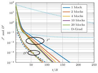
Figure 1: Distance from stationarity $J^{t}$ (solid) and consensus disagreement $D^{t}$ (dashed) versus the normalized number of iterations for several choices of the blocks’ number $B$ of Block-SONATA-PL.

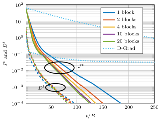
Figure 2: Distance from stationarity $J^{t}$ (solid) and consensus disagreement $D^{t}$ (dashed) versus the normalized number of iterations for several choices of the blocks’ number $B$ of Block-SONATA-L.

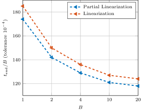
Figure 3: Normalized completion time to obtain $J^{t}<10^{-4}$ versus the number of blocks $B$, for Block-SONATA-PL and Block-SONATA-L.

V Conclusions

In this paper we proposed a novel block-iterative distributed scheme for nonconvex, big-data optimization problems over (directed) networks. The key novel feature of the scheme is a block-wise minimization from the agents of a convex approximation of the sum-utility, coupled with a block-wise consensus/tracking mechanism aiming to average both the local copies of the agents’ decision variables and the local estimates of the cost-function gradient. Asymptotic convergence to a stationary solution of the problem as well as consensus of the agents’ local variables was proved.

References

• [1] Y. Nesterov, “Efficiency of coordinate descent methods on huge-scale optimization problems,” SIAM Journal on Optimization, vol. 22, no. 2, pp. 341–362, 2012.
• [2] P. Richtárik and M. Takáč, “Parallel coordinate descent methods for big data optimization,” Mathematical Programming, pp. 1–52, 2012.
• [3] ——, “Iteration complexity of randomized block-coordinate descent methods for minimizing a composite function,” Mathematical Programming, vol. 144, no. 1-2, pp. 1–38, 2014.
• [4] I. Necoara and D. Clipici, “Parallel random coordinate descent method for composite minimization: Convergence analysis and error bounds,” SIAM Journal on Optimization, vol. 26, no. 1, pp. 197–226, 2016.
• [5] F. Facchinei, G. Scutari, and S. Sagratella, “Parallel selective algorithms for nonconvex big data optimization,” IEEE Transactions on Signal Processing, vol. 63, no. 7, pp. 1874–1889, 2015.
• [6] L. Cannelli, F. Facchinei, V. Kungurtsev, and G. Scutari, “Asynchronous parallel algorithms for nonconvex big-data optimization$-$Part I: Model and convergence,” arXiv preprint arXiv:1607.04818, 2016.
• [7] A. Mokhtari, A. Koppel, and A. Ribeiro, “Doubly random parallel stochastic methods for large scale learning,” in American Control Conference (ACC).   IEEE, 2016, pp. 4847–4852.
• [8] H. R. Feyzmahdavian, A. Aytekin, and M. Johansson, “An asynchronous mini-batch algorithm for regularized stochastic optimization,” IEEE Transactions on Automatic Control, vol. 61, no. 12, pp. 3740–3754, 2016.
• [9] I. Necoara, “Random coordinate descent algorithms for multi-agent convex optimization over networks,” IEEE Transactions on Automatic Control, vol. 58, no. 8, pp. 2001–2012, 2013.
• [10] A. Nedić and A. Olshevsky, “Distributed optimization over time-varying directed graphs,” IEEE Transactions on Automatic Control, vol. 60, no. 3, pp. 601–615, 2015.
• [11] M. Akbari, B. Gharesifard, and T. Linder, “Distributed online convex optimization on time-varying directed graphs,” IEEE Transactions on Control of Network Systems, 2015.
• [12] K. Margellos, A. Falsone, S. Garatti, and M. Prandini, “Distributed constrained optimization and consensus in uncertain networks via proximal minimization,” arXiv preprint arXiv:1603.02239, 2016.
• [13] P. D. Lorenzo and G. Scutari, “Distributed nonconvex optimization over networks,” in IEEE International Conference on Computational Advances in Multi-Sensor Adaptive Processing (CAMSAP), 2015.
• [14] P. Di Lorenzo and G. Scutari, “NEXT: In-network nonconvex optimization,” IEEE Transactions on Signal and Information Processing over Networks, vol. 2, no. 2, pp. 120–136, 2016.
• [15] Y. Sun, G. Scutari, and D. Palomar, “Distributed nonconvex multiagent optimization over time-varying networks,” in IEEE Asilomar Conference on Signals, Systems, and Computers, 2016.
• [16] Y. Sun and G. Scutari, “Distributed nonconvex optimization for sparse representation,” in IEEE International Conference on Speech and Signal Processing (ICASSP), 2017.
• [17] A. Nedić, A. Olshevsky, and W. Shi, “A geometrically convergent method for distributed optimization over time-varying graphs,” in IEEE 55th Conference on Decision and Control (CDC), 2016, pp. 1023–1029.
• [18] G. Qu and N. Li, “Harnessing smoothness to accelerate distributed optimization,” in IEEE Conference on Decision and Control (CDC), 2016, pp. 159–166.
• [19] F. Zanella, D. Varagnolo, A. Cenedese, G. Pillonetto, and L. Schenato, “Asynchronous Newton-Raphson consensus for distributed convex optimization,” in 3rd IFAC Workshop on Distributed Estimation and Control in Networked Systems, 2012.
• [20] R. Carli, G. Notarstefano, L. Schenato, and D. Varagnolo, “Analysis of Newton-Raphson consensus for multi-agent convex optimization under asynchronous and lossy communications,” in IEEE Conference on Decision and Control (CDC), 2015, pp. 418–424.
• [21] R. Carli and G. Notarstefano, “Distributed partition-based optimization via dual decomposition,” in IEEE Conference on Decision and Control (CDC), 2013, pp. 2979–2984.
• [22] I. Notarnicola and G. Notarstefano, “A randomized primal distributed algorithm for partitioned and big-data non-convex optimization,” in IEEE Conference on Decision and Control (CDC), 2016, pp. 153–158.
• [23] C. Wang, Y. Zhang, B. Ying, and A. H. Sayed, “Coordinate-descent diffusion learning by networked agents,” arXiv preprint arXiv:1607.01838, 2016.
• [24] P. Bianchi and J. Jakubowicz, “Convergence of a multi-agent projected stochastic gradient algorithm for non-convex optimization,” IEEE Transactions on Automatic Control, vol. 58, no. 2, pp. 391–405, 2013.