Flexible and Robust Particle Tempering for State Space Models

Abstract

Density tempering (also called density annealing) is a sequential Monte Carlo approach to Bayesian inference for general state models; it is an alternative to Markov chain Monte Carlo. When applied to state space models, it moves a collection of parameters and latent states (which are called particles) through a number of stages, with each stage having its own target distribution. The particles are initially generated from a distribution that is easy to sample from, e.g. the prior; the target at the final stage is the posterior distribution. Tempering is usually carried out either in batch mode, involving all the data at each stage, or sequentially with observations added at each stage, which is called data tempering. Our paper proposes efficient Markov moves for generating the parameters and states for each stage of particle based density tempering. This allows the proposed SMC methods to increase (scale up) the number of parameters and states that can be handled. Most of the current literature uses a pseudo-marginal Markov move step with the states “integrated out,”and the parameters generated by a random walk proposal; although this strategy is general, it is very inefficient when the states or parameters are high dimensional. We also build on the work of Dufays, (2016) and make data tempering more robust to outliers and structural changes for models with intractable likelihoods by adding batch tempering at each stage. The performance of the proposed methods is evaluated using univariate stochastic volatility models with outliers and structural breaks and high dimensional factor stochastic volatility models having both many parameters and many latent states.

Keywords: Factor stochastic volatility model; Hamiltonian Monte Carlo; Outliers; Structural change; Particle Markov chain Monte Carlo; Diffusion process

1 Introduction

Joint inference over both the parameters and latent states in nonlinear and non-Gaussian state space models is challenging because the likelihood is usually an intractable integral over the latent states. In a seminal contribution, Andrieu et al., (2010) propose two batch particle Markov chain Monte Carlo (PMCMC) methods for state space models. The first method is the particle marginal Metropolis-Hastings (PMMH), where the parameters are generated with the unobserved latent states “integrated out”; this technically means that the likelihood is replaced by its unbiased estimate. The second method is the particle Gibbs (PG), which generates the parameters conditional on the states and conversely. Both methods run a particle filter algorithm within an MCMC sampling scheme at each iteration. Andrieu et al., show that for any finite number of particles, the augmented target density used by these two algorithms has the joint posterior distribution of the parameters and states as its marginal distribution. A number of papers, including Lindsten and Schon, (2013), Lindsten et al., (2014), Olsson and Ryden, (2011), Mendes et al., (2020), and Gunawan et al., 2020a , extend their work.

Density tempering sequential Monte Carlo (SMC) is an alternative to MCMC as a computational approach for Bayesian inference. It is a sequential importance sampling approach (Neal,, 2001), where samples are first drawn from an easily-generated distribution, e.g., the prior, and then moved towards the target distribution through a sequence of intermediate stages, with each stage having its own target distribution. Del Moral et al., (2006) outline the sequential Monte Carlo (SMC) method, which consists of resampling, reweighting and Markov move steps at each stage of the SMC.

It is generally recognised (Del Moral et al.,, 2006) that SMC has the following advantages compared to MCMC, and in particular, PMCMC approaches: (a) the Markov chain generated by an PMCMC sampler often gets trapped in local modes; it is also difficult to assess whether the chain mixes adequately and converges to its invariant distribution. SMC explores the parameter space more efficiently when the target distribution is multimodal; assessing convergence is also easier. (b) It is usually difficult to use PMCMC to estimate the marginal likelihood, which is often used to for model choice (Kass and Raftery,, 1995; Chib and Jeliazkov,, 2001). Using SMC to estimate the marginal likelihood is more straightforward. Section 4.2 also shows the usefulness of the sequential SMC approach to estimate the sequence of independent standard normal random variables used to form the goodness of fit statistics to test for the model adequacy of a general time series state space model as in Smith, (1985), Shephard, (1994), and Gerlach et al., (1998). Using PMCMC to compute the goodness of fit statistics can be very time-consuming as it is necessary to repeatedly construct the full Markov chain for each time period $t$; see, for example, Gerlach et al., (1998). (c) PMCMC algorithms are not parallelisable in general, whereas SMC algorithms can be parallelised (subject to some caveats); see, for example, Neal, (2001), Del Moral et al., (2006), and Duan and Fulop, (2015). Section 2.2 discusses this further.

Duan and Fulop, (2015) extend the annealing/density tempering method of Neal, (2001), and Del Moral et al., (2006) to time series state space models having intractable likelihoods. Their approach processes the time series as a batch. Fulop and Li, (2013) and Chopin et al., (2013) propose full sequential Bayesian inference on the parameters and call their algorithm Marginalised Resample-Move (MRM) and $\textrm{SMC}^{2}$, respectively.

Our paper builds on this literature by proposing flexible SMC approaches that use Markov move steps that are more efficient than the density tempered SMC approach of Duan and Fulop, (2015), MRM of Fulop and Li, (2013), and $\textrm{SMC}^{2}$ of Chopin et al., (2013). The first Markov move approach is based on the PG algorithm of Andrieu et al., (2010); we call it sequential Monte Carlo with particle Gibbs (SMC-PG). The second is based on the Hamiltonian Monte Carlo (HMC) algorithm (Duane et al.,, 1987; Neal,, 2011; Girolami and Calderhead,, 2011; Hoffman and Gelman,, 2014; Betancourt,, 2017); we call it sequential Monte Carlo with Hamiltonian Monte Carlo (SMC-HMC). The third is based on the particle hybrid sampler of Gunawan et al., 2020a , which combines a step similar to the correlated PMMH of Deligiannidis et al., (2018) and the particle Gibbs of Andrieu et al., (2010); we call it sequential Monte Carlo with the particle hybrid sampler (SMC-PHS). The Markov move step based on PHS generates the parameters that are highly correlated with the states in PMMH steps. All other parameters are generated by particle Gibbs steps conditioning on the latent state variables.

The Markov moves based on PG, PHS and HMC are important for two reasons. First, they permit applications to much higher dimensional parameter spaces and much better proposals than random walk proposals; in particular, in some cases we are able to sample from the full conditional distribution using Gibbs steps. Second, Section 5.2 shows that using particle Gibbs Markov moves can substantially reduce the number of particles required because it is then unnecessary for the variance of the log of the likelihood estimate to be in the range of 1 to 3. In addition, if we suspect that some parameters converge slowly because they are highly correlated with the latent states in the model, then they can be generated using the PMMH step of the PHS.

Dufays, (2016) robustifies data tempering by adding batch tempering at each data point. His approach is suitable for models with a tractable likelihood enabling the Markov move steps to be carried out by MCMC. The target densities in Dufays, depend only on the parameters and the method is applied to standard GARCH models and GARCH models with change-point, and both only have a few parameters. Our article extends Dufays,’s approach to handle state space models with intractable likelihoods and with the latent states also appearing in the target densities; this makes it possible to obtain joint inference on both the parameters and the latent states.

Section 4.3 and Section 10.2 of the Supplement show that the proposed SMC is more stable than the methods of Fulop and Li, (2013) and Chopin et al., (2013) in datasets with outliers and structural breaks because it incorporates information from the data more gradually.

Our proposed sequential approach with tempering is different to previous approaches. It provides joint sequential inference on latent states and parameters up to time $t$, $p(\bm{x}_{1:t},\bm{\theta}|\bm{y}_{1:t})$, whereas the $\textrm{SMC}^{2}$ provides sequential inference on the parameters only. Johansen, (2015) does not propose density tempering or data tempering or a combination of both for making inference on the parameters, states, or both. Johansen, proposes a block tempered particle filter to estimate the likelihood unbiasedly and provides the filtered state distribution $p(\bm{x}_{1:t}|\bm{y}_{1:t},\bm{\theta})$. Johansen, mentions that the block tempered particle filter can be used within the PMCMC for making inference on the parameters of the state space models, although he does not show it. His particle filter algorithm can also be used within our SMC algorithm, although we do not pursue this idea.

The Markov move step in SMC helps to diversify the particles to provide a better approximation to the tempered target distribution at that temperature level. Duan and Fulop, (2015), Fulop and Li, (2013) and Chopin et al., (2013) use a particle marginal Metropolis-Hastings (PMMH) approach with the likelihood estimated unbiasedly by the particle filter in the Markov move step. There are two drawbacks to a Markov move based on PMMH. First, it is computationally costly to follow the guidelines of Pitt et al., (2012) for high dimensional state space models and set the optimal number of particles in the particle filter such that the variance of the log of the estimated likelihood is in the range of $1$ to $3$; see the empirical example in Section 5.2. It is possible to implement the correlated PMMH of Deligiannidis et al., (2018), which is more efficient than standard PMMH for low dimensional state space models. However, the correlated PMMH is ineffective for a model with a high dimensional state, e.g. the factor SV model in Section 5.2. Second, it is hard to implement the PMMH Markov move efficiently for a high dimensional parameter as it is difficult to obtain a good proposal for the parameter because the first and second derivatives with respect to the parameters can only be estimated. Nemeth et al., (2016) and Mendes et al., (2020) find that the behaviour of the particle Metropolis adjusted Langevin algorithm (MALA) depends critically on how accurately we can estimate the gradient of the log-posterior. If the variance of the estimate of the gradient of the log-posterior is too large, then there is no advantage in using particle MALA over the random walk proposal. The random walk proposal is easy to implement, but is very inefficient in high dimensions.

We illustrate the proposed SMC methods empirically using a sample of daily US stock returns to estimate the univariate stochastic volatility (SV) models with outliers and structural breaks and the multivariate high dimensional factor SV model. The factor SV model is popular because it parsimoniously models a vector of returns. Most applications of multivariate factor stochastic volatility models are in financial econometrics (Nardari and Scruggs,, 2007; Aguilar and West,, 2000; Zhou et al.,, 2014). Current popular MCMC estimation approaches for the factor SV model by Chib et al., (2006) and Kastner et al., (2017) are neither exact nor flexible; neither paper corrects for the approximation errors. They follow the approach proposed by Kim et al., (1998) to approximate the distribution of log outcome innovations by a carefully constructed seven component mixture of normal distributions. In the empirical application in Section 5.2, we show that the MCMC sampler of Kastner et al., (2017) can give very different results to the PHS for some parameters of the factor SV model. The accuracy of the proposed SMC approaches are also compared to the PHS. Section 5.2 shows that the proposed SMC samplers give accurate estimates of the posterior densities of the parameters and predictive densities. We also consider a factor SV with the log-volatilities of the idiosyncratic errors to follow continuous time Ornstein-Uhlenbeck (OU) processes (Stein and Stein,, 1991). Although the continuous time OU diffusion model has a closed form transition density (Brix et al.,, 2018), the SMC methods are applied to the Euler approximation of the OU process and hence can handle the diffusion processes that do not admit closed form transition densities (Ignatieva et al.,, 2015). Section 5.3 gives further details.

The rest of the article is organised as follows. Section 2 outlines the state space model and its estimation by SMC. Section 3 discusses the proposed flexible Markov moves. Section 4 presents empirical results for the univariate example. Section 5 introduces and presents empirical results for the factor SV model. The online Supplement to the paper contains some further technical and empirical results.The following notation is used in both the main paper and the online Supplement. Eq. (1), Section 1, Algorithm 1 and Sampling Scheme 1, etc. refer to the main article, while Eq. (S1), Section S1, Algorithm S1, and Sampling Scheme S1, etc. refer to the Supplement.

2 Flexible Density Tempering

This section introduces the state space model and discusses the SMC approaches.

2.1 The State Space Model

We use the colon notation for collections of variables, i.e. $\bm{a}_{t}^{1:N}=\left(a_{t}^{1},...,a_{t}^{N}\right)$, $\bm{a}_{1:t}^{1:N}=\left(\bm{a}_{1}^{1:N},...,\bm{a}_{t}^{1:N}\right)$, and $\bm{a}_{1:M,1:t}=\left(a_{1,1},...,a_{M,1},a_{1,2},...,a_{M,2},...,a_{1,t},...,a_{M,t}\right)$.

We consider a state space model where the latent states $\bm{X}_{t}$ determine the evolution of the system. The density of $\bm{X}_{1}$ is $p\left(\bm{x}_{1}|\bm{\theta}\right)$ and the transition density of $\bm{X}_{t}$ given $\bm{X}_{1:t-1}=\bm{x}_{1:t-1}$ is $p\left(\bm{x}_{t}|\bm{x}_{t-1},\bm{\theta}\right)$ for $t\geq 2$. The observations $\bm{Y}_{t}=\bm{y}_{t}$ for $t=1,...,T$ are linked to the latent states through the observation equation $p\left(\bm{y}_{t}|\bm{x}_{t},\bm{\theta}\right)$. Denote the $d$-dimensional Euclidean space by $\mathbb{R}^{d}$. We suppose that (i) the state vector $\bm{x}_{t}\in\mathcal{X}$ and the observation $\bm{y}_{t}\in\mathcal{Y}$, where $\mathcal{X}\subset\mathbb{R}^{d_{x}}$ and $\mathcal{Y}\subset\mathbb{R}^{d_{y}}$; (ii) the parameter vector $\bm{\theta}\in\bm{\Theta}$, where $\bm{\Theta}$ is a subset of $\mathbb{R}^{d_{\theta}}$.

Our aim is to perform Bayesian inference over the latent states and the parameters conditional on the observations $\bm{y}_{1:T}$. By using Bayes rule, the joint posterior of the latent states and the parameters is

$$p\left(\bm{\theta},\bm{x}_{1:T}|\bm{y}_{1:T}\right) =\frac{p\left(\bm{x}_{1:T},\bm{y}_{1:T}|\bm{\theta}\right)p\left(\bm{\theta}\right)}{p\left(\bm{y}_{1:T}\right)},$$

$$\text{where}\quad p\left(\bm{x}_{1:T},\bm{y}_{1:T}|\bm{\theta}\right) =p\left(\bm{x}_{1}|\bm{\theta}\right)\prod_{t=2}^{T}p\left(\bm{x}_{t}|\bm{x}_{t-1},\bm{\theta}\right)\prod_{t=1}^{T}p\left(\bm{y}_{t}|\bm{x}_{t},\bm{\theta}\right);$$

$p\left(\bm{\theta}\right)$ is the prior density of $\bm{\theta}$ and $p\left(\bm{y}_{1:T}\right)$ is the marginal likelihood of $\bm{y}_{1:T}$. For notational simplicity, we often write $\bm{x}=\bm{x}_{1:T}$ and $\bm{y}=\bm{y}_{1:T}$.

Examples

This section illustrates the state space model by the univariate stochastic volatility model,

$$y_{t} =\exp\left(x_{t}/2\right)\epsilon_{t},\quad x_{t+1}=\mu+\phi\left(x_{t}-\mu\right)+\tau\eta_{t+1},\quad x_{1}\sim N\left(\mu,\frac{\tau^{2}}{1-\phi^{2}}\right),$$ (1)

with $\epsilon_{t}\sim N\left(0,1\right)$ and $\eta_{t}\sim N\left(0,1\right)$ and independent. We call $\bm{x}_{1:T}$ the latent log volatility process. The vector of unknown parameters is $\bm{\theta}=(\mu,\phi,\tau^{2})$. To ensure that the model is stationary, we restrict the persistence parameter $\phi$ so that $|\phi|<1$.

2.2 The SMC Approach for State Space Models

2.2.1 Batch Estimation Method

This section discusses the proposed SMC method for batch estimation problems. The main idea is to begin with an easy-to-sample distribution and propagate a particle cloud $\left\{\bm{\theta}_{1:M}^{\left(p\right)},\bm{x}_{1:M}^{\left(p\right)},\bm{W}_{1:M}^{\left(p\right)}\right\}$ through a sequence of tempered target densities $\xi_{a_{p}}\left(\bm{\theta},\bm{x}\right)$, for $p=0,...,P$, to the posterior density of interest which is much harder to sample from directly. The tempered densities are defined as

$$\xi_{a_{p}}\left(\bm{\theta},\bm{x}\right) :=\eta_{a_{p}}\left(\bm{\theta},\bm{x}\right)/Z_{a_{p}},\quad\text{where}\quad Z_{a_{p}}:=\int\eta_{a_{p}}\left(\bm{\theta},\bm{x}\right)d\bm{\theta}d\bm{x}$$

$$\text{and}\quad\eta_{a_{p}}\left(\bm{\theta},\bm{x}\right) :=\left(\pi_{0}\left(\bm{\theta},\bm{x}\right)\right)^{1-a_{p}}\left(p\left(\bm{y}|\bm{\theta},\bm{x}\right)p\left(\bm{x}|\bm{\theta}\right)p\left(\bm{\theta}\right)\right)^{a_{p}}.$$

The tempering sequence $\bm{a}_{0:P}$ is such that $a_{0}=0<a_{1}<...<a_{P}=1$. If it is both easy to generate from the densities $p\left(\bm{\theta}\right)$ and $p\left(\bm{x}|\bm{\theta}\right)$, and evaluate them, then we take $\pi_{0}\left(\bm{x},\bm{\theta}\right)=p\left(\bm{\theta}\right)p\left(\bm{x}|\bm{\theta}\right)$, and hence

$$\eta_{a_{p}}\left(\bm{\theta},\bm{x}\right)=p\left(\bm{y}|\bm{\theta},\bm{x}\right)^{a_{p}}p\left(\bm{x}|\bm{\theta}\right)p\left(\bm{\theta}\right).$$ (2)

Algorithm 1 summarizes the general SMC approach, which we now discuss. The initial particle cloud $\left\{\bm{\theta}_{1:M}^{\left(0\right)},\bm{x}_{1:M}^{\left(0\right)},\bm{W}_{1:M}^{\left(0\right)}\right\}$ is obtained by generating the $\left\{\bm{\theta}_{1:M}^{\left(0\right)},\bm{x}_{1:M}^{\left(0\right)}\right\}$ from $\pi_{0}\left(\bm{x},\bm{\theta}\right)$, and giving the particles equal weight, i.e., $\bm{W}_{1:M}^{\left(0\right)}=1/M$. The weighted particles (particle cloud) $\left\{\bm{\theta}_{1:M}^{\left(p-1\right)},\bm{x}_{1:M}^{\left(p-1\right)},\bm{W}_{1:M}^{\left(p-1\right)}\right\}$ at the $\left(p-1\right)$st level (or stage) of the annealing is an estimate of $\xi_{a_{p-1}}\left(\bm{\theta},\bm{x}\right)$. Based on this estimate of $\xi_{a_{p-1}}\left(\bm{\theta},\bm{x}\right)$, the SMC algorithm goes through the following steps to obtain an estimate of $\xi_{a_{p}}\left(\bm{\theta},\bm{x}\right)$. The move from $\xi_{a_{p-1}}\left(\bm{\theta},\bm{x}\right)$ to $\xi_{a_{p}}\left(\bm{\theta},\bm{x}\right)$ is implemented by reweighting the particles by the ratio of the two unnormalized densities $\eta_{a_{p}}/\eta_{a_{p-1}}$, yielding the following weights, $\bm{W}_{1:M}^{\left(p\right)}=\bm{w}^{(p)}_{1:M}/\sum_{j=1}^{M}w^{(p)}_{j}$, where

$$w^{(p)}_{i}=W_{i}^{\left(p-1\right)}\frac{\eta_{a_{p}}\left(\bm{\theta}^{(p-1)}_{i},\bm{x}^{(p-1)}_{i}\right)}{\eta_{a_{p-1}}\left(\bm{\theta}^{(p-1)}_{i},\bm{x}^{(p-1)}_{i}\right)}=W_{i}^{\left(p-1\right)}p\left(\bm{y}|\bm{\theta}^{(p-1)}_{i},\bm{x}^{(p-1)}_{i}\right)^{a_{p}-a_{p-1}},$$ (3)

where $\eta_{a_{p}}$ is defined in Eq. (2). We follow Del Moral et al., (2012) and choose the tempering sequence adaptively to ensure sufficient particle diversity by selecting the next value of $a_{p}$ automatically such that the effective sample size (ESS) stays close to some target value $\textrm{ESS}_{\textrm{target}}$ chosen by the user. The ESS is used to measure the variability in the $W_{i}^{(p)}$, and is defined as $\textrm{ESS}:={\left(\sum_{i=1}^{M}\left(W_{i}^{(p)}\right)^{2}\right)}^{-1}$. The ESS varies between 1 and $M$, with a low value of ESS indicating that the weights are concentrated only on a few particles and a value of $M$ means that the particles are equally weighted. An ESS close to the target value is achieved by evaluating the ESS over a grid $\bm{a}_{1:G,p}$ of potential $a_{p}$ values and selecting as $a_{p}$ the value of $a_{j,p}$ whose ESS is the closest to $\textrm{ESS}_{\textrm{target}}$. Other approaches to select the tempering sequence, such as that in Del Moral et al., (2012), may be used instead. The particles $\left\{\bm{\theta}_{1:M}^{\left(p\right)},\bm{x}_{1:M}^{\left(p\right)}\right\}$ are then resampled proportionately to their weights $\bm{W}_{1:M}^{\left(p\right)}$, which means that the resampled particles then have equal weight $\bm{W}_{1:M}^{\left(p\right)}=1/M$. This has the effect of eliminating particles with negligible weights and replicating the particles with large weights, so the ESS is now $M$. We use multinomial resampling for all the examples in the paper.

Repeatedly reweighting and resampling can seriously reduce the diversity of the particles, and lead to particle depletion. The particle cloud $\left\{\bm{\theta}_{1:M}^{\left(p\right)},\bm{x}_{1:M}^{\left(p\right)},\bm{W}_{1:M}^{\left(p\right)}\right\}$ may then be a poor representation of $\xi_{a_{p}}\left(\bm{\theta},\bm{x}\right)$. To improve the approximation of the particle cloud to $\xi_{a_{p}}\left(\bm{\theta},\bm{x}\right)$, we carry out $R$ Markov move steps for each particle using a Markov kernel $K_{a_{p}}$ which retains $\xi_{a_{p}}\left(\bm{\theta},\bm{x}\right)$ as its invariant density. Thus, at each annealing level, we run a short MCMC scheme for each of the $M$ particles.

Steps $1$ and 2a-2d of Algorithm 1 are standard and apply to any model, with only slight model-specific modifications; hence, it is only necessary to discuss the Markov move step in detail for each model. We propose three Markov move algorithms that leave the target density $\xi_{a_{p}}\left(\bm{\theta},\bm{x}\right)$ invariant. The first algorithm is based on particle Gibbs (Andrieu et al.,, 2010), and is denoted as SMC-PG. The second algorithm is based on Hamiltonian Monte Carlo (Neal,, 2011), and is denoted as SMC-HMC. The third algorithm is based on the particle hybrid sampler (PHS) of Gunawan et al., 2020a , and is denoted as SMC-PHS.

By Del Moral et al., (2006), the SMC algorithm provides consistent inference for the target density $p\left(\bm{\theta},\bm{x}_{1:T}|\bm{y}_{1:T}\right)$ as $M$ goes to infinity. See also Beskos et al., (2016) for recent consistency results for the adaptive algorithm employed here and the associated central limit theorem.

Section 1 states that the SMC algorithm can be parallelised. However, parallelising SMC is not straightforward due to the resampling in step (2d) of Alg. 1. In our applications given in Sections 4 and 5.2, the optimal number of annealing levels, $P$, obtained from the adaptive approach described above is moderate and therefore resampling has little effect on the efficiency of the SMC algorithm. The reweighting in step (2c) and the Markov moves in step (2e) are easily parallelised for each SMC sample because the computations required for each sample are independent ofthe other SMC samples.

Algorithm 1 Generic SMC Algorithm

1. Set $p=0$ and initialise the particle cloud $\left\{\bm{\theta}_{1:M}^{\left(0\right)},\bm{x}_{1:M}^{\left(0\right)},\bm{W}_{1:M}^{\left(0\right)}\right\}$, by generating the $\left\{\bm{\theta}_{1:M}^{\left(0\right)},\bm{x}_{1:M}^{\left(0\right)}\right\}$ from $\pi_{0}\left(\bm{x},\bm{\theta}\right)$, and giving them equal weight, i.e., $W_{i}^{\left(0\right)}=1/M$, for $i=1,...,M$

2. While the tempering sequence $a_{p}<1$ do

   1. Set $p\leftarrow p+1$

   2. Find $a_{p}$ adaptively by searching across a grid of $a_{p}$ values to maintain ESS around some constant $\textrm{ESS}_{\textrm{target}}$.

   3. Compute new weights,

      $$\bm{W}_{1:M}^{\left(p\right)}=\frac{\bm{w}^{(p)}_{1:M}}{\sum_{j=1}^{M}w^{(p)}_{j}}\;\;\textrm{where}\;\;w^{(p)}_{i}=W_{i}^{\left(p-1\right)}\frac{\eta_{a_{p}}\left(\bm{\theta_{i}}^{(p-1)},\bm{x_{i}}^{(p-1)}\right)}{\eta_{a_{p-1}}\left(\bm{\theta_{i}}^{(p-1)},\bm{x_{i}}^{(p-1)}\right)}.$$ (4)

   4. Resample $\left(\bm{\theta}_{i}^{\left(p-1\right)},\bm{x}_{i}^{\left(p-1\right)}\right)$ using the weights $\bm{W}_{1:M}^{\left(p\right)}$ to obtain $\left\{\bm{\theta}_{1:M}^{\left(p\right)},\bm{x}_{1:M}^{\left(p\right)},\bm{W}_{1:M}^{\left(p\right)}=1/M\right\}$.

   5. Markov moves

      1. Let $K_{a_{p}}\left(\left(\bm{\theta},\bm{x}\right),\cdot\right)$ be a Markov kernel having invariant density $\xi_{a_{p}}\left(\bm{\theta},\bm{x}\right)$. For $i=1,...,M$, move each $\left(\bm{\theta}_{i}^{\left(p\right)},\bm{x}_{i}^{\left(p\right)}\right)$ $R$ times using the Markov kernel $K_{a_{p}}$ to obtain $\left\{\widetilde{\bm{\theta}}_{i},\widetilde{\bm{x}}_{i}\right\}$.

      2. Set $\left(\bm{\theta}_{1:M}^{\left(p\right)},\bm{x}_{1:M}^{\left(p\right)}\right)\leftarrow\left(\widetilde{\bm{\theta}}_{1:M},\widetilde{\bm{x}}_{1:M}\right)$.

2.2.2 Sequential Estimation Method

We now discuss the extension of the density tempered SMC approach in Section 2.2.1 to the situation where we are interested in sequential estimation of both the states and parameters as new observations arrive. This approach has very useful applications, especially in finance and economics. For example, in finance, investors need to update their volatility and return forecasts whenever new data become available. As another example, economists need to revise their forecasts as news on the state of the economy changes. Here, PMCMC techniques are expensive and time-consuming to use as they need to repeatedly restart the MCMC as new observations arrive.

The main challenge is how to jointly sample and propagate the states and parameters as new observations arrive. Our framework deals with this by extending the SMC sequence of target distributions as the number of observations increases. The main idea is to propagate a particle cloud $\left\{\bm{\theta}_{1:M}^{\left(p\right)},\bm{x}_{1:t-1,1:M}^{\left(p\right)},\bm{W}_{1:M}^{\left(p\right)}\right\}$ that reflects the joint posterior of states $\bm{x}_{1:t-1}$ and parameters $\bm{\theta}$ at time $t-1$ through a sequence of tempered target densities $\xi_{a_{p}}\left(\bm{\theta},\bm{x}\right)$, for $p=0,...,P$, to the joint posterior density of states $\bm{x}_{1:t}$ and parameters $\bm{\theta}$ at time $t$. The tempered densities are defined as

$$\xi_{a_{p}}\left(\bm{\theta},\bm{x}_{1:t}\right):=\eta_{a_{p}}\left(\bm{\theta},\bm{x}_{1:t}\right)/Z_{a_{p}},\;\;\textrm{where}\;\;Z_{a_{p}}:=\int\eta_{a_{p}}\left(\bm{\theta},\bm{x}_{1:t}\right)d\bm{\theta}d\bm{x}_{1:t},\\ \textrm{and}\;\eta_{a_{p}}\left(\bm{\theta},\bm{x}\right):=p\left(\bm{y}_{t}|\bm{x}_{t},\bm{\theta}\right)^{a_{p}}p\left(\bm{x}_{t}|\bm{x}_{t-1},\bm{\theta}\right)p\left(\bm{\theta},\bm{x}_{1:t-1}|\bm{y}_{1:t-1}\right).$$

The move from $\xi_{a_{p-1}}\left(\bm{\theta},\bm{x}_{1:t-1}\right)$ to $\xi_{a_{p}}\left(\bm{\theta},\bm{x}_{1:t}\right)$ is implemented by reweighting the particles by the ratio of the two unnormalised densities $\eta_{a_{p}}/\eta_{a_{p-1}}$, yielding the weights

$$w_{i}^{\left(p\right)}:=W_{i}^{\left(p-1\right)}\frac{\eta_{a_{p}}\left(\bm{\theta}_{i}^{\left(p-1\right)},\bm{x}_{i,1:t}^{\left(p-1\right)}\right)}{\eta_{a_{p-1}}\left(\bm{\theta}_{i}^{\left(p-1\right)},\bm{x}_{i,1:t}^{\left(p-1\right)}\right)}=W_{i}^{\left(p-1\right)}p\left(\bm{y}_{t}|\bm{x}^{(p-1)}_{i,t},\bm{\theta}^{(p-1)}_{i}\right)^{a_{p}-a_{p-1}}.$$

Section 4.3 and Supplement 10.2 show that our sequential approach is robust to outliers and structural breaks; this happens because tempering incorporates the information in new observations gradually. It also means that it is easy to maintain the ESS close to its target $\textrm{ESS}_{\textrm{target}}$.

The $\textrm{SMC}^{2}$ sequential approach in Chopin et al., (2013) only targets the posterior density $p(\bm{\theta}|\bm{y}_{1:t})$ of the parameters $\bm{\theta}$ by “integrating out” the latent states, $\bm{x}_{1:t}$, up to time $t$. Our sequential tempering approach targets the joint posterior density $p(\bm{\theta},\bm{x}_{1:t}|\bm{y}_{1:t})$ of the parameters $\bm{\theta}$ and latent states, $\bm{x}_{1:t}$, up to time $t$.

3 Flexible Markov Moves

This section discusses the Markov move steps in step (2e) of Algorithm 1. The first is based on the Hamiltonian Monte Carlo (HMC) algorithm (Neal,, 2011). The second is based on the particle Gibbs (PG) algorithm of Andrieu et al., (2010). The third is based on the particle marginal Metropolis-Hastings (PMMH) algorithm of Andrieu et al., (2010). The fourth is based on the particle hybrid sampler of Gunawan et al., 2020a .

3.1 Hamiltonian Monte Carlo

The Markov move has two steps. The first step updates the latent states $\bm{x}_{1:T}$ conditional on the parameters $\bm{\theta}$ using Hamiltonian Monte Carlo (HMC). The second step updates the parameters $\bm{\theta}$ conditional on the states $\bm{x}_{1:T}$.

Sampling the high dimensional latent state vector $\bm{x}_{1:T}$ is discussed first. Suppose we want to sample from a $T$-dimensional distribution with a density proportional to $\exp\left(\mathcal{L}\left(\bm{x}\right)\right)$, where $\mathcal{L}\left(\bm{x}\right)=\log p\left(\bm{x}|\bm{\theta},\bm{y}\right)$. In Hamiltonian Monte Carlo (Neal,, 2011), we augment $\bm{x}$ with an auxiliary momentum vector $\bm{r}$, having the same dimension as the latent state vector $\bm{x}$, with the density $p\left(\bm{r}\right)=N\left(\bm{r}|0,\widetilde{M}\right)$, where $\widetilde{M}$ is a mass matrix. We define the joint conditional density of $\left(\bm{x},\bm{r}\right)$ as

$$p\left(\bm{x},\bm{r}|\textrm{rest}\right) \propto\exp\left(-H\left(\bm{x},\bm{r}\right)\right),$$

where $H\left(\bm{x},\bm{r}\right)=-\mathcal{L}\left(\bm{x}\right)+\frac{1}{2}\bm{r}^{T}\widetilde{M}^{-1}\bm{r}$ is called the Hamiltonian. In an idealised Hamiltonian step, the state vector $\bm{x}$ and the momentum variables $\bm{r}$ move continuously according to the differential equations

$$\frac{d\bm{x}}{dt}=\frac{\partial H}{\partial\bm{r}}=\widetilde{M}^{-1}\bm{r},\frac{d\bm{r}}{dt}=-\frac{\partial H}{\partial\bm{x}}=\nabla_{\bm{x}}\mathcal{L}\left(\bm{x}\right),$$

where $\nabla_{\bm{x}}$ denotes the gradient with respect to $\bm{x}$. In practice, this continuous time Hamiltonian dynamics needs to be approximated by discretizing time, using a step size $\epsilon$. We can then simulate the evolution over time of $\left(\bm{x},\bm{r}\right)$ via the “leapfrog” integrator using Alg. 2.

Sections 9.1 and 9.2 of the Supplement give the details for the univariate SV model. Sections 13.1 and 13.2 of the Supplement give the details for the factor SV model.

Algorithm 2 The Hamiltonian Monte Carlo part of a single Markov move step (Hoffman et al.,, 2013)

Given initial values of $\bm{x}$, $\epsilon$, $L$, where $L$ is the number of leapfrog updates

Sample $\bm{r}\sim N\left(0,\widetilde{M}\right)$

For $l=1$ to $L$

Set $\left(\bm{x}^{*},\bm{r}^{*}\right)\leftarrow\textrm{Leapfrog}\left(\bm{x},\bm{r},\epsilon\right)$

end for

With probability

$$\alpha =\min\left(1,\frac{\exp\left(\mathcal{L}\left(\bm{x}^{*}\right)-\frac{1}{2}\bm{r}^{*T}\widetilde{M}^{-1}\bm{r}^{*}\right)}{\exp\left(\mathcal{L}\left(\bm{x}\right)-\frac{1}{2}\bm{r}^{T}\widetilde{M}^{-1}\bm{r}\right)}\right),$$

set $\bm{x}=\bm{x}^{*}$, $\bm{r}^{*}=-\bm{r}$, else retain current $\bm{x}$.

function Leapfrog($\bm{x}$,$\bm{r}$,$\epsilon$)
Set $\bm{r}+\epsilon\nabla_{\bm{x}}\mathcal{L}\left(\bm{x}\right)/2$
Set $\bm{x}+\epsilon\bm{\widetilde{M}}^{-1}\bm{r}$,
Set $\bm{r}+\epsilon\nabla_{\bm{x}}\mathcal{L}\left(\bm{x}\right)/2$,
return $\bm{x}^{*}$, $\bm{r}^{*}$

3.2 Particle Gibbs

The Markov moves based on PG, PMMH, and PHS run a particle filter algorithm at each iteration. Section 3.2.1 discusses the particle filter. Section 3.2.2 then discusses particle Gibbs based Markov move steps.

3.2.1 Particle Filter

This section describes the particle filter methods used to obtain sequential approximations to the densities $p\left(\bm{x}_{1:t}|\bm{y}_{1:t},\bm{\theta}\right)$ for $t=1,...,T$. The particle filter algorithm recursively produces a set of weighted particles $\left\{\bm{x}_{1:t}^{\left(j\right)},\widetilde{W}_{t}^{\left(j\right)}\right\}_{j=1}^{N}$ such that the intermediate densities $p\left(\bm{x}_{1:t}|\bm{y}_{1:t},\bm{\theta}\right)$ are approximated by

$$\widehat{p}\left(\bm{x}_{1:t}|\bm{y}_{1:t},\bm{\theta}\right)=\sum_{j=1}^{N}\widetilde{W}_{t}^{\left(j\right)}\delta_{\bm{x}_{1:t}^{(j)}}\left(d\bm{x}_{1:t}\right),$$

where $\delta_{a}\left(dx\right)$ is the Dirac delta distribution located at $a$. In more detail, given $N$ samples $\left\{\bm{x}_{t-1}^{\left(j\right)},\widetilde{W}_{t-1}^{\left(j\right)}\right\}_{j=1}^{N}$ representing the filtering density $p\left(\bm{x}_{t-1}|\bm{y}_{1:t-1},\bm{\theta}\right)$ at time $t-1$, we use

$$p\left({x}_{t}|\bm{y}_{1:t},\bm{\theta}\right)\propto\int p\left({y}_{t}|{x}_{t},\bm{\theta}\right)p\left({x}_{t}|{x}_{t-1},\bm{\theta}\right)p\left({x}_{t-1}|\bm{y}_{1:t-1},\bm{\theta}\right)d{x}_{t-1},$$

to obtain the particles $\left\{{x}_{t}^{\left(j\right)},\widetilde{W}_{t}^{\left(j\right)}\right\}_{j=1}^{N}$ representing $p({x}_{t}|\bm{y}_{1:t},\bm{\theta})$, by first drawing from a known and easily sampled proposal density function $m\left({x}_{t}|{x}_{t-1},{y}_{t},\bm{\theta}\right)$ and then computing the unnormalised weights $\widetilde{w}_{t}^{(j)}$ to account for the difference between the target posterior density and the proposal, where

$$\widetilde{w}_{t}^{\left(j\right)}:=\widetilde{W}_{t-1}^{(j)}\frac{p\left({y}_{t}|{x}_{t}^{\left(j\right)},\bm{\theta}\right)p\left({x}_{t}^{\left(j\right)}|{x}_{t-1}^{\left(j\right)},\bm{\theta}\right)}{m_{t}\left({x}_{t}^{\left(j\right)}|{x}_{t-1}^{\left(j\right)},{y}_{t},\bm{\theta}\right)},\;j=1,...,N;$$

these are then normalized as $\widetilde{W}_{t}^{\left(j\right)}:=\widetilde{w}_{t}^{\left(j\right)}/\sum_{r=1}^{N}\widetilde{w}_{t}^{\left(r\right)}$.

Chopin, (2004) shows that as the number of time periods $t$ increases, the normalised weights of the particle system become concentrated only on a few particles and eventually the normalised weight of a single particle converges to one. This is known as the ‘weight degeneracy’ problem. One way to reduce the impact of weight degeneracy is to include resampling steps in a particle filter algorithm. A resampling scheme is defined as ${\cal M}\left(\widetilde{\bm{b}}_{t-1}^{1:N}|\widetilde{\bm{W}}_{t-1}^{1:N}\right)$, where $\widetilde{b}_{t-1}^{j}$ indexes a particle in $\left\{{x}_{t-1}^{\left(j\right)},\widetilde{W}_{t-1}^{\left(j\right)}\right\}_{j=1}^{N}$ that is chosen with probability $\widetilde{W}_{t-1}^{\left(j\right)}$. Section 16 of the Supplement states some assumptions on the proposal density $m_{t}\left({x}_{t}|{x}_{t-1},{y}_{t},\bm{\theta}\right)$ and resampling scheme. In our empirical applications, we use the bootstrap filter with $p\left({x}_{t}|{x}_{t-1},\bm{\theta}\right)$ as a proposal density and multinomial resampling.

The particle filter produces the unbiased estimate of the likelihood

$$\widehat{p}\left(\bm{y}_{1:T}|\bm{\theta}\right) =\widehat{p}\left({y}_{1}|\bm{\theta}\right)\prod_{t=2}^{T}\widehat{p}\left({y}_{t}|{y}_{t-1},\bm{\theta}\right)=\prod_{t=1}^{T}\left\{\frac{1}{N}\sum_{j=1}^{N}\widetilde{w}_{t}^{(j)}\right\},$$

i.e. $\mathrm{E}\left(\widehat{p}\left(\bm{y}_{1:T}|\bm{\theta}\right)\right)=p\left(\bm{y}_{1:T}|\bm{\theta}\right)$ (Del Moral,, 2004; Pitt et al.,, 2012).

3.2.2 Particle Gibbs (PG) Algorithm

This section discusses the Markov move based on the particle Gibbs algorithm. Unless stated otherwise, we write PG to denote both the particle Gibbs (PG) and particle Metropolis within Gibbs Markov moves. Let $\bm{U}_{1:T}^{1:N}=\left(\bm{x}_{1:T}^{1:N},\widetilde{\bm{b}}_{1:T-1}^{1:N}\right)$ denote the collection of particles in the particle filter algorithm, together with their associated indices $\widetilde{\bm{b}}_{1:T-1}^{1:N}$ defined in Section 3.2.1. The SMC-PG constructs a sequence of tempered densities $\xi_{a_{p}}\left(\bm{\theta},\bm{x}_{1:T}\right)$, $p=1,...,P$, based on the augmented tempered target density that includes all the particles generated by the particle filter. Section 11 of the Supplement gives further details of the augmented tempered target density.

Algorithm 3 gives the Markov move based on the particle Gibbs algorithm. Let $\bm{\theta}\coloneqq\left(\bm{\theta}_{1},...,\bm{\theta}_{H}\right)$ be a partition of the parameter vector into $H$ components, where each component may be a vector.

Algorithm 3 Markov move based on the Particle Gibbs algorithm

For $i=1,...,M$ SMC samples,

1. For $h=1,...,H$, sample $\bm{\theta}_{ih}^{*}$ from the proposal density
   $q_{h}\left(\cdot|\bm{j}_{i,1:T},\bm{x}_{i,1:T}^{\bm{j}_{i,1:T}},\bm{\theta}_{-ih},\bm{\theta}_{ih}\right)$.

2. Accept the proposed values $\bm{\theta}_{ih}^{*}$ with probability

   $$\min\left(1,\frac{\xi_{a_{p}}\left(\bm{\theta}_{ih}^{*}|\bm{x}_{i,1:T}^{\bm{j}_{i,1:T}},\bm{j}_{i,1:T},\bm{\theta}_{-ih}\right)}{\xi_{a_{p}}\left(\bm{\theta}_{ih}|\bm{x}_{i,1:T}^{\bm{j}_{i,1:T}},\bm{j}_{i,1:T},\bm{\theta}_{-ih}\right)}\frac{q_{h}\left(\bm{\theta}_{ih}|\bm{\theta}_{-ih},\bm{\theta}_{ih}^{*},\bm{x}_{i,1:T}^{\bm{j}_{i,1:T}},\bm{j}_{i,1:T}\right)}{q_{h}\left(\bm{\theta}_{ih}^{*}|\bm{\theta}_{-ih},\bm{\theta}_{ih},\bm{x}_{i,1:T}^{\bm{j}_{i,1:T}},\bm{j}_{i,1:T}\right)}\right).$$

3. Sample $\bm{U}_{i,1:T}^{\left(-\bm{j}_{i,1:T}\right)}$ using conditional sequential Monte Carlo given in Algorithm 9 in Section 15 of the Supplement.

4. Sample $J_{i,t}=j_{i,t}\sim\widetilde{\xi}_{a_{p}}\left(\bm{j}_{i,1:T}|\bm{x}_{i,1:t}^{1:N},\widetilde{\bm{b}}_{i,1:t-1}^{1:N},\bm{\theta}_{i},\bm{x}_{i,t+1:T}^{\bm{j}_{i,t+1:T}},\bm{j}_{i,t+1:T}\right)$ for
   $t=T-1,...,1$ and $J_{i,T}=j_{i,T}\sim\widetilde{\xi}_{a_{p}}\left(j_{i,T}|\bm{\theta}_{i},\bm{x}_{i,1:T}^{1:N},\widetilde{\bm{b}}_{i,1:T-1}^{1:N}\right)$ using the backward simulation algorithm given in Algorithm 10 of Section 15 of the supplement.

Parts 1 and 2 of Algorithm 3 update each parameter block of $\bm{\theta}$ conditional on a trajectory $\bm{x}_{1:T}^{\bm{j}_{1:T}}=\left(x_{1}^{j_{1}},...,x_{T}^{j_{T}}\right)$. Part 3 is the conditional sequential Monte Carlo of Andrieu et al., (2010) that is the key part of the Markov move steps. It is a particle filter algorithm in which a particle $\bm{x}_{1:T}^{\bm{j}_{1:T}}=\left(\bm{x}_{1}^{j_{1}},...,\bm{x}_{T}^{j_{T}}\right)$, and the associated sequence of ancestral indices are kept unchanged with all the other particles and indices resampled and updated. The collection of all random variables except the chosen particle trajectory is denoted by $\bm{U}_{1:T}^{-\bm{j}_{1:T}}$. Part 4 of Algorithm 3 samples the new indices $J_{T},J_{T-1},...,J_{1}$ sequentially using backward simulation given in Algorithm 10 of Section 15 of the Supplement, obtains the new particle trajectory $\bm{x}_{1:T}^{\bm{j}_{1:T}}=\left(x_{1}^{j_{1}},...,x_{T}^{j_{T}}\right)$, and discards the rest of the particles. Following Whiteley, (2010) and Lindsten and Schon, (2013), the conditional density in Part 4 is

$$\widetilde{\xi}_{a_{p}}\left(j_{t}|\bm{\theta},{x}_{1:t}^{1:N},\widetilde{\bm{b}}_{1:t-1}^{1:N},\bm{x}_{t+1:T}^{\bm{j}_{t+1:T}},\bm{j}_{t+1:T}\right)\propto\widetilde{w}_{t}^{j_{t}}p\left(\bm{x}_{t+1}^{j_{t+1}}|\bm{\theta},\bm{x}_{t}^{j_{t}}\right),$$

for $t=T-1,...,1$ and $\widetilde{\xi}_{a_{p}}\left(j_{T}|\bm{\theta},\bm{x}_{1:T}^{1:N},\widetilde{\bm{b}}_{1:T-1}^{1:N}\right)\propto\widetilde{w}_{T}^{j_{T}}$. The Markov move based on the PG algorithm is useful in generating the vector of high-dimensional parameters, except when some of the parameters are highly correlated with the latent states.

3.3 Particle Marginal Metropolis-Hastings

Algorithm 4 describes the Markov move based on the particle marginal Metropolis-Hastings (PMMH) approach (Andrieu et al.,, 2010); this is useful for generating parameters that are highly correlated with the states. The PMMH algorithm requires an unbiased estimate of the likelihood, which is obtained from the particle filter.

Algorithm 4 Particle Marginal Metropolis-Hastings (PMMH) Algorithm

Given initial values for $\bm{U}_{i,1:T}$, $\bm{\theta}_{i}$, and $\bm{j}_{i,1:T}$, for $i=1,...,M$ SMC samples. One iteration of PMMH involves the following steps:

1. Sample $\bm{\theta}_{i}^{*}$ from the proposal density $q\left(\bm{\theta}_{i}^{*}|\bm{\theta}_{i},\bm{U}_{i,1:T}\right)$.

2. Sample $\bm{U}_{i,1:T}^{*}\sim\psi\left(\bm{U}_{i,1:T}^{*}|\bm{\theta}_{i}^{*}\right)$ by running the particle filter algorithm in Algorithm 8 of Section  15 of the Supplement and compute a tempered estimate of the likelihood $\widehat{p}\left(\bm{y}_{1:T}|\bm{\theta}_{i}^{*}\right)^{a_{p}}$.

3. Sample $J_{i,1:T}^{*}=j_{i,1:T}^{*}$ using the backward simulation algorithm given in Algorithm 10 of Section  15 of the Supplement.

4. Accept the proposed values of $\bm{\theta}_{i}^{*}$, $\bm{U}_{i,1:T}^{*}$, and $\bm{j}^{*}_{i,1:T}$ with probability

   $$\min\left\{1,\frac{\widehat{p}\left(\bm{y}_{1:T}|\bm{\theta}_{i}^{*}\right)^{a_{p}}p\left(\bm{\theta}_{i}^{*}\right)}{\widehat{p}\left(\bm{y}_{1:T}|\bm{\theta}_{i}\right)^{a_{p}}p\left(\bm{\theta}_{i}\right)}\frac{q\left(\bm{\theta}_{i}|\bm{\theta}_{i}^{*}\right)}{q\left(\bm{\theta}_{i}^{*}|\bm{\theta}_{i}\right)}\right\}.$$ (5)

Parts 1 to 3 of the Algorithm 4 propose the values of $\bm{\theta}_{i}^{*}$, $\bm{U}_{i,1:T}^{*}\sim\psi\left(\bm{U}_{i,1:T}^{*}|\bm{\theta}_{i}^{*}\right)$, and $\bm{j}_{i,1:T}^{*}$, which are then accepted with the probability in Eq. (5). Algorithm 4 targets the joint posterior density of the latent states $\bm{x}_{1:T}$ and the parameters $\bm{\theta}$. Duan and Fulop, (2015) use a PMMH method, with the likelihood estimated unbiasedly by the particle filter, in the Markov move component. However, they only target the posterior distribution of the parameters $\bm{\theta}$. We call their method SMC-PMMH-DF.

3.4 Particle Hybrid Sampler

Mendes et al., (2020) propose a new particle MCMC sampler that combines the particle Gibbs and PMMH algorithms of Andrieu et al., (2010). The sampler generates parameters that are highly correlated with the states using PMMH, with the rest generated by PG. Deligiannidis et al., (2018) propose the correlated PMMH method, which correlates the random numbers used in constructing the likelihood estimates at the current and proposed values of the parameters. They show that the correlated PMMH can scale up with the number of observations compared to standard PMMH, as long as the state dimension is not too large. Gunawan et al., 2020a propose a novel PMCMC which involves a non-trivial combination of the correlated PMMH and the PG algorithms; Gunawan et al., 2020a call it the particle hybrid sampler (PHS). Unlike Andrieu et al., (2010), its augmented target density is expressed in terms of basic uniform and standard normal random numbers. The parameters that are efficiently generated by conditioning on the latent states are generated in a particle Gibbs step. All other parameters are drawn with PMMH steps by conditioning on the basic uniform and standard normal variables used in the particle filter algorithm. The PHS sampler is scalable in the number of observations and the number of parameters. See Gunawan et al., 2020a for further details.

The PHS Sampling Scheme

Algorithm 5 outlines the Markov move steps based on the particle hybrid sampler. For simplicity, let $\bm{\theta}\coloneqq\left(\bm{\theta}_{1},\bm{\theta}_{2}\right)$ partition the parameter vector into 2 components. It generates $\bm{\theta}_{1}$ using a PMMH step and the vector parameter $\bm{\theta}_{2}$ using a PG step. The elements in $\bm{\theta}_{1}$ and $\bm{\theta}_{2}$ are sampled separately in the PMMH step and PG step, respectively.

Algorithm 5 The Particle Hybrid Sampler (PHS).

Given initial values for $\bm{v}_{x,i,1:T}^{1:N}$, $\bm{v}_{B,i,1:T-1}$, $\bm{j}_{i,1:T}$, and $\bm{\theta}_{i}$. For $i=1,...,M$ (SMC samples), one iteration of the PHS involves the following steps:

1. PMMH sampling.

   1. Sample $\bm{\theta}_{i,1}^{*}\sim q_{1}\left(\cdot|\bm{\theta}_{i,2},\bm{\theta}_{i,1}\right)$

   2. Run the particle filter with Euclidean sort in Algorithm 13 of Section 15.2 of the Supplement and evaluate $\widehat{p}(\bm{y}_{1:T}|\bm{\theta}^{*}_{i,1},\bm{\theta}_{i,2})^{a_{p}}$.

   3. Accept the proposed values $\bm{\theta}_{i,1}^{*}$ with probability

      $$\alpha\left(\bm{\theta}_{i,1};\bm{\theta}_{i,1}^{*}|\bm{u}_{x,i,1:T}^{1:N},\bm{u}_{A,i,1:T-1},\bm{\theta}_{i,2}\right) =$$

      $$1\land\frac{\widehat{p}(\bm{y}_{1:T}|\bm{\theta}^{*}_{i,1},\bm{\theta}_{i,2})^{a_{p}}p\left(\bm{\theta}_{i,1}^{*}|\bm{\theta}_{i,2}\right)}{\widehat{p}(\bm{y}_{1:T}|\bm{\theta}_{i,1},\bm{\theta}_{i,2})^{a_{p}}p\left(\bm{\theta}_{i,1}|\bm{\theta}_{i,2}\right)} \times\frac{q_{1}\left(\bm{\theta}_{i,1}|\bm{\theta}_{i,2},\bm{\theta}_{i,1}^{*}\right)}{q_{1}\left(\bm{\theta}_{i,1}^{*}|\bm{\theta}_{i,2},\bm{\theta}_{i,1}\right)}.$$ (6)

2. Sample $\bm{J}_{i,1:T}=\bm{j}_{i,1:T}$ using the backward simulation algorithm given in Algorithm 10 of Section 15 of the Supplement.

3. Particle Gibbs (PG) sampling.

   1. Sample $\bm{\theta}_{i,2}^{*}\sim q_{2}\left(\cdot|\bm{\theta}_{i,1},\bm{\theta}_{i,2}\right)$

   2. Accept the proposed values $\bm{\theta}_{i,2}^{*}$ with probability

      $$\alpha\left(\bm{\theta}_{i,2};\bm{\theta}_{i,2}^{*}|\bm{x}_{i,1:T}^{j_{i,1:T}},\bm{j}_{i,1:T},\bm{\theta}_{i,1}\right)$$

      $$= 1\land\frac{p\left(\bm{y}_{1:T}|\bm{x}_{i,1:T}^{j_{i,1:T}},\bm{\theta}_{i,2}^{*},\bm{\theta}_{i,1}\right)^{a_{p}}p\left(\bm{x}_{i,1:T}^{j_{i,1:T}}|\bm{\theta}_{i,2}^{*},\bm{\theta}_{i,1}\right)p\left(\bm{\theta}_{i,2}^{*}|\bm{\theta}_{i,1}\right)}{p\left(\bm{y}_{1:T}|\bm{x}_{i,1:T}^{j_{i,1:T}},\bm{\theta}_{i,2},\bm{\theta}_{i,1}\right)^{a_{p}}p\left(\bm{x}_{i,1:T}^{j_{i,1:T}}|\bm{\theta}_{i,2},\bm{\theta}_{i,1}\right)p\left(\bm{\theta}_{i,2}|\bm{\theta}_{i,1}\right)}$$

      $$\times\frac{q_{2}\left(\bm{\theta}_{i,2}|\bm{\theta}_{i,1},\bm{\theta}_{i,2}^{*}\right)}{q_{2}\left(\bm{\theta}_{i,2}^{*}|\bm{\theta}_{i,1},\bm{\theta}_{i,2}\right)}.$$

4. Sample $\left(\bm{v}_{i,x,1:T},\bm{v}_{i,A,1:T-1}\right)$ using the constrained conditional sequential Monte Carlo algorithm (Algorithm 11 of Section 15.1) of the Supplement and evaluate $\widehat{p}(\bm{y}_{1:T}|\bm{\theta}_{i,1},\bm{\theta}_{i,2})^{a_{p}}$.

Part 1 generates $\bm{\theta_{1}}^{*}$ using PMMH, conditioning on the random numbers $\bm{v}_{x,1:T}^{1:N}$ and $\bm{v}_{B,1:T-1}$ obtained from Part 4, the parameters $\bm{\theta}_{2}$, and the current parameters $\bm{\theta}_{1}$. Part 2 samples the new indices $\bm{j}_{1:T}$ using the backward simulation algorithm, obtains the new particle trajectory $\bm{x}_{1:T}^{\bm{j}_{1:T}}=\left(x_{1}^{j_{1}},...,x_{T}^{j_{T}}\right)$, and discards the rest of the particles. Part 3 generates the parameters $\bm{\theta}^{*}_{2}$ using PG, conditioning on the selected particle trajectory $\bm{x}_{1:T}^{\bm{j}_{1:T}}$, the parameter $\bm{\theta}_{1}$ and the current parameter $\bm{\theta}_{2}$. Part 4 updates the basic random numbers using constrained conditional sequential Monte Carlo (Gunawan et al., 2020a, ); see Section  15.1 of the Supplement.

3.5 Marginal Likelihood Estimation

The marginal likelihood $p\left(\bm{y}_{1:T}\right)$ is often used in the Bayesian literature to compare models (Chib and Jeliazkov,, 2001). An advantage of the SMC method is that it offers a natural way to estimate the marginal likelihood. We note that $p\left(\bm{y}_{1:T}\right)=Z_{a_{P}}$, $Z_{a_{0}}=1$, so that

$$p\left(\bm{y}_{1:T}\right)=\prod_{p=1}^{P}\frac{Z_{a_{p}}}{Z_{a_{p-1}}}\;\;\textrm{with}\;\;\frac{Z_{a_{p}}}{Z_{a_{p-1}}}=\int\left(\frac{\eta_{a_{p}}\left(\bm{\theta},\bm{x}\right)}{\eta_{a_{p-1}}\left(\bm{\theta},\bm{x}\right)}\right)\xi_{a_{p-1}}\left(\bm{\theta},\bm{x}\right)d\bm{\theta}d\bm{x}.$$

Because the particle cloud $\left\{\bm{\theta}_{1:M}^{\left(p-1\right)},\bm{x}_{1:M}^{\left(p-1\right)},\bm{W}_{1:M}^{\left(p-1\right)}\right\}$ obtained after iteration $p-1$ approximates $\xi_{a_{p-1}}\left(\bm{\theta},\bm{x}\right)$, the ratio above is estimated by

$$\widehat{\frac{Z_{a_{p}}}{Z_{a_{p-1}}}}=\sum_{i=1}^{M}W_{i}^{\left(p-1\right)}\frac{\eta_{a_{p}}\left(\bm{\theta}_{i}^{\left(p-1\right)},\bm{x}_{i}^{\left(p-1\right)}\right)}{\eta_{a_{p-1}}\left(\bm{\theta}_{i}^{\left(p-1\right)},\bm{x}_{i}^{\left(p-1\right)}\right)},$$

giving the marginal likelihood estimate

$$\widehat{p\left(\bm{y}_{1:T}\right)}=\prod_{p=1}^{P}\widehat{\frac{Z_{a_{p}}}{Z_{a_{p-1}}}}.$$

4 Univariate Examples

4.1 Univariate Stochastic Volatility Model

This section illustrates the proposed SMC-PG and SMC-HMC methods for batch estimation problems by applying them to the univariate stochastic volatility (SV) model and compares their performance to the exact particle hybrid sampler (PHS) of Gunawan et al., 2020a and the SMC-PMMH-DF of Duan and Fulop, (2015). Posterior distributions obtained from the PHS method are treated as the ‘ground truth’ for comparing the accuracy of the posterior density approximations for two reasons. The first is that we have extensively applied PHS to stochastic volatility models, and in our experience it has always worked well. Second, PHS belongs to the class of PMCMC methods of Andrieu et al., (2010) and their key property is that they are an ‘exact approximation’ to the idealised MCMC algorithms targeting the joint posterior density of the latent states and parameters $p(\bm{x}_{1:T},\bm{\theta}|y_{1:T})$ (Andrieu et al.,, 2010). We follow South et al., (2019) and Gunawan et al., 2020b by comparing the posterior densities of the parameters estimated using different SMC algorithms and exact MCMC methods.

The vector of unknown parameters of the SV model in Section 2.1 is $\bm{\theta}=(\mu,\phi,\tau^{2})$. The parameters have the following priors, and are assumed to be independent apriori: (a) $p\left(\mu\right)\propto I\left(-10<\mu<10\right)$. (b) Following Jensen and Maheu, (2010), the prior for $\tau^{2}$ is inverse Gamma $\textrm{IG}\left(v_{0}/2,s_{0}/2\right)$ with $v_{0}=10$ and $s_{0}=0.5$. (c) To ensure stationarity, the persistence parameter is restricted to $\mid\phi\mid<1$; we follow Kim et al., (1998) and choose the prior for $\phi$ as $\left(\phi+1\right)/2\sim\textrm{Beta}\left(a_{0},b_{0}\right)$, with $a_{0}=100$ and $b_{0}=1.5$. We apply our methods to a sample of daily US food industry stock returns obtained from the Kenneth French website, using a sample from December 11th, 2001 to the 11th November 2013, a total of $3001$ observations.

The performance of SMC-HMC depends on choosing suitable values for the three tuning parameters i) the mass matrix $\widetilde{M}$, ii) the step size $\epsilon$, and iii) the number of leapfrog steps $L$. The step size $\epsilon$ determines how well the leapfrog integration approximates the Hamiltonian dynamics. If it is too large, then a low acceptance rate may result, but if it is too small, then it becomes computationally expensive to obtain distant proposals. Similarly, if $L$ is too small, then the proposal will be close to the current value of the latent state vectors, resulting in undesirable random walk behaviour. If $L$ is too large, then HMC will generate proposals that retrace their steps. The precision matrix $\Sigma^{-1}$ of the AR(1) process of the latent states is a sparse tridiagonal matrix whose diagonal elements are $0.5a_{p}+\left(1+\phi^{2}\right)/\tau^{2}$, except for the first and last diagonal elements which are $0.5a_{p}+1/\tau^{2}$; the super- and sub-diagonal elements are $-{\phi}/{\tau^{2}}$. We set $\widetilde{M}=\Sigma^{-1}$. Our article uses two adaptive approaches. The first follows an adaptive method based on Garthwaite et al., (2015) to select an $\epsilon$ that yields a specified average acceptance probability across all $M$ particles and $L$ is set to some fixed value; we denote this method as SMC-HMC-I. The second adaptive approach is to select both $\epsilon$ and $L$ based on the adaptive method by Buchholz et al., (2020) and denote it as SMC-HMC-II.

Table 1 summarises the estimation results for the univariate SV model estimated using the PHS, SMC-HMC, SMC-PG, and SMC-PMMH-DF methods. The PHS chain consists of 5000 iterates for burnin and another 50000 iterates used for inference. All the SMC estimates are obtained using 10 independent runs, each with $M=560$ samples, to generate a total of $5600$ samples for each algorithm. We set the constant $\textrm{ESS}_{T}=0.8M$. The computations are done using Matlab on a single desktop computer with 6-CPU cores.

Table 1 shows that all the SMC-PG estimates are very close to the PHS estimates for all parameters even with as few as $150$ particles and $R=10$ Markov move steps. The middle panel of Fig. 1 shows the kernel density estimates of the marginal posteriors of the univariate stochastic volatility parameters $\tau^{2}$ estimated using the PHS and the SMC-PG methods with different numbers of particles. The density estimates from the SMC-PG methods are very close to the density estimates of the PHS sampler.

Table 1 shows that the estimates of $\tau^{2}$ and $\phi$ estimated using the SMC-HMC-I with $R=20$ is the closest to the estimates of the PHS compared to SMC-HMC-I with $R=10$ and SMC-HMC-II. But in general, they are very close to each other. The right panel of Fig. 1 shows the kernel density estimates of the marginal posteriors of the univariate SV parameters $\tau^{2}$ estimated using the PHS and the SMC-HMC methods. The figure confirms that the densities estimates of $\tau^{2}$ estimated from SMC-HMC-I with $R=20$ are the closest to the estimates from the PHS, but still sligthly inaccurate compared to the SMC-PG estimates. In general, SMC-PG is more accurate than the SMC-HMC, but its CPU time is slightly larger. Table 1 also shows that the optimal number of Markov move steps obtained from the adaptive approach described in Section 2.2 are similar for SMC-PG and SMC-HMC methods.

The left panel of Fig. 1 shows the kernel density estimates of the marginal posteriors of the univariate SV parameters $\tau^{2}$ estimated using the PHS and the SMC-PMMH-DF methods. The density estimates from SMC-PMMH-DF with $N=2000$ and $5000$ particles are close to the PHS estimates. The number of Markov move steps of SMC-PMMH-DF are smaller compared to the SMC-PG and SMC-HMC methods because it only targets the posterior density of SV parameters and not the latent log-volatilities. The SMC-PG with $N=250$ particles is still slightly faster than SMC-PMMH-DF with $N=2000$ particles.

Fig. 2 shows the posterior mean estimates of the latent log-volatilities estimated using PHS with $N=100$, SMC-PG with $N=250$, SMC-HMC-I with $R=20$, and SMC-PMMH-DF with $N=2000$. The SMC-PG, SMC-PMMH-DF, and PHS estimates are indistinguishable. The estimates from SMC-HMC-I are slightly less accurate at some time points. This study suggets that (a) The SMC-HMC methods are less accurate compared to SMC-PG and SMC-PMMH-DF methods for estimating the standard univariate SV models; (b) The SMC-PG with $N=250$ is as accurate as the SMC-PMMH-DF with $N=2000$, and faster than the SMC-PMMH-DF for this example; (c) The SMC-PMMH-DF provides inference only on the parameters, and not the latent states. Two steps are needed to obtain the posterior density of the latent states. First, the SMC draws of the parameters are obtained from running the SMC-PMMH-DF algorithm. Second, the particle filter and backward simulation algorithms are run for each parameter draw to give the posterior density of the latent states.

Table 1: Results for the univariate SV model estimated using the PHS, SMC-HMC, SMC-PG, and SMC-PMMH-DF samplers for the US food stock returns data with $T=3001$. The SMC results are obtained using 10 independent runs of each algorithm. Time is the time in minutes for one run of the algorithm. The posterior standard deviations of the SV parameters are in brackets.

Method	$N$	$L$	$R$	$\mu$	$\phi$	$\tau^{2}$	$P$	Time
PHS	100	-	-	$\underset{\left(0.2054\right)}{-0.4886}$	$\underset{\left(0.0040\right)}{0.9853}$	$\underset{\left(0.0040\right)}{0.0226}$	-	513
HMC-I	-	100	10	$\underset{\left(0.1992\right)}{-0.4934}$	$\underset{\left(0.0043\right)}{0.9839}$	$\underset{\left(0.0041\right)}{0.0252}$	57	62.87
HMC-I	-	100	20	$\underset{\left(0.2007\right)}{-0.4888}$	$\underset{\left(0.0039\right)}{0.9849}$	$\underset{\left(0.0039\right)}{0.0234}$	57	123.68
HMC-II	-	100	20	$\underset{\left(0.2006\right)}{-0.4959}$	$\underset{\left(0.0045\right)}{0.9839}$	$\underset{\left(0.0051\right)}{0.0253}$	57	137.23
PG	150	-	10	$\underset{\left(0.2096\right)}{-0.4996}$	$\underset{\left(0.0040\right)}{0.9850}$	$\underset{\left(0.0040\right)}{0.0231}$	59	109.27
PG	250	-	10	$\underset{\left(0.2106\right)}{-0.4986}$	$\underset{\left(0.0041\right)}{0.9851}$	$\underset{\left(0.0040\right)}{0.0229}$	57	156.18
PMMH-DF	500	-	10	$\underset{\left(0.2185\right)}{-0.4590}$	$\underset{\left(0.0040\right)}{0.9852}$	$\underset{\left(0.0041\right)}{0.0234}$	15	58.03
PMMH-DF	1000	-	10	$\underset{\left(0.2052\right)}{-0.4802}$	$\underset{\left(0.0040\right)}{0.9855}$	$\underset{\left(0.0039\right)}{0.0229}$	14	105.63
PMMH-DF	2000	-	10	$\underset{\left(0.2059\right)}{-0.4797}$	$\underset{\left(0.0041\right)}{0.9850}$	$\underset{\left(0.0041\right)}{0.0229}$	14	226.18
PMMH-DF	5000	-	10	$\underset{\left(0.2038\right)}{-0.4878}$	$\underset{\left(0.0040\right)}{0.9853}$	$\underset{\left(0.0040\right)}{0.0228}$	13	671.94

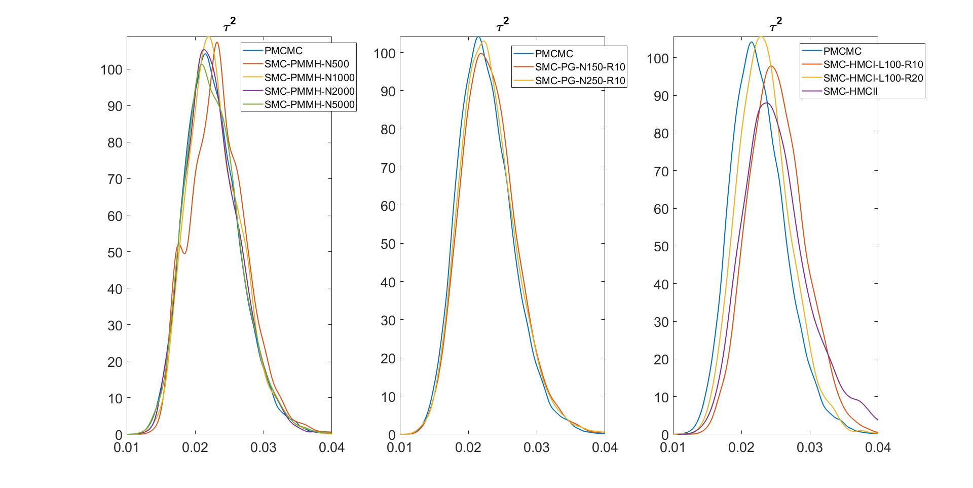
Figure 1: The kernel density estimates of the marginal posterior densities of the univariate SV parameters $\tau^{2}$ estimated using SMC-PMMH-DF (left), SMC-PG (middle), and SMC-HMC (right). Each method is compared with PHS (PMCMC).

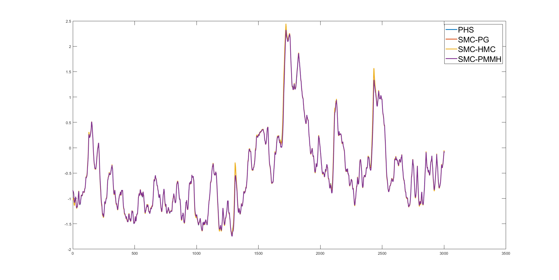
Figure 2: Standard univariate stochastic volatility example. The plots of the log-volatility estimates using the PHS (with $N=100$), SMC-PG ($N=250$), SMC-HMC-I ( $R=20$), and SMC-PMMH-DF ($N=2000$).

The above analyses suggest that for this example the SMC-PG and SMC-PMMH-DF are the most accurate SMC methods. The next example compares the performance of the SMC-PG and SMC-PMMH-DF for estimating the univariate SV model with a larger number of parameters. The measurement equation is now

$$y_{t}=\bm{l}_{t}^{\top}\bm{\beta}+\exp\left(x_{t}/2\right)\epsilon_{t},\;\textrm{where}\;\;\epsilon_{t}\sim{\cal N}\left(0,1\right),$$ (7)

where $\bm{\beta}=(\beta_{1},...,\beta_{50})^{\top}$ and $l_{t}=(l_{1,t},...,l_{50,t})^{\top}$ is a $(50\times 1)$ vector of covariates at time $t$. We compare the performance of the following samplers: (I) the PHS with $N=100$, (II) SMC-PG with $N=250$, (III) SMC-PMMH-DF with $N=1000$ and $2500$. We apply the methods to simulated data with $T=6000$ observations, $\phi=0.99$, $\tau^{2}=0.5$, $\rho=-0.2$, $\mu=0.5$. The parameters $\beta_{k}$ are generated independently of each other from normal distributions with mean zero and standard deviation $1$, for all $k=1,...,50$. The covariates are generated randomly from a multivariate normal ${\cal N}(\bm{0},I)$. The prior for $\beta_{k}$ is ${\cal N}(0,1)$ for $k=1,...,50$.

Fig. 3 shows the kernel density estimates of some marginal posterior densities of the univariate SV parameters with the covariate coefficients estimated using the PHS, the SMC-PMMH-DF and the SMC-PG methods. The figure shows that the SMC-PG estimates are very close to the PHS estimates for all SV parameters and the three covariate coefficients $(\beta_{1},\beta_{2},\beta_{3})$. The estimates from the SMC-PMMH-DF are different to the PHS even with $N=2500$ particles. Similar conclusions hold for other $\beta$ coefficients given in Figure 14 of Supplement 10. Table 2 summarizes the estimation results of the SV model with covariates. Interestingly, the number of Markov move steps for the SMC-PMMH-DF is similar to the SMC-PG method for this example. The SMC-PG method is more accurate and 4.76 times faster than the SMC-PMMH-DF with $N=2500$ particles.

This example suggests that (a) The SMC-PG performs better than the SMC-PMMH-DF for estimating the univariate SV parameters with covariate coefficients. The vector of parameters $\beta$ are high dimensional and not highly correlated with the states, so it is efficient to generate them in a PG step. (b) SMC-PMMH-DF gives different estimates to the PHS even with $N=2500$ particles. SMC-PMMH-DF uses a PMMH approach with a random walk proposal for the parameters in the Markov move component. The random walk is easy to implement, but is not efficient for high-dimensional parameters. However, SMC-PMMH-DF is a more general algorithm than SMC-PG. It only needs an efficient estimate of the likelihood. Section 5.3 discusses an example that uses the SMC-PHS method where it is useful to generate parameters that are highly correlated with the states using PMMH steps and the other parameters are generated using PG steps by conditioning on the states.

Table 2: Simulated data with $T=6000$ for the univariate SV with covariates estimated using the SMC-PG and SMC-PMMH-DF samplers. Time is in minutes for one run of the algorithm.

Method	N	R	P	Time
PG	250	10	89	754.79
PMMH-DF	1000	10	72	1081.29
PMMH-DF	2500	10	72	3590.80

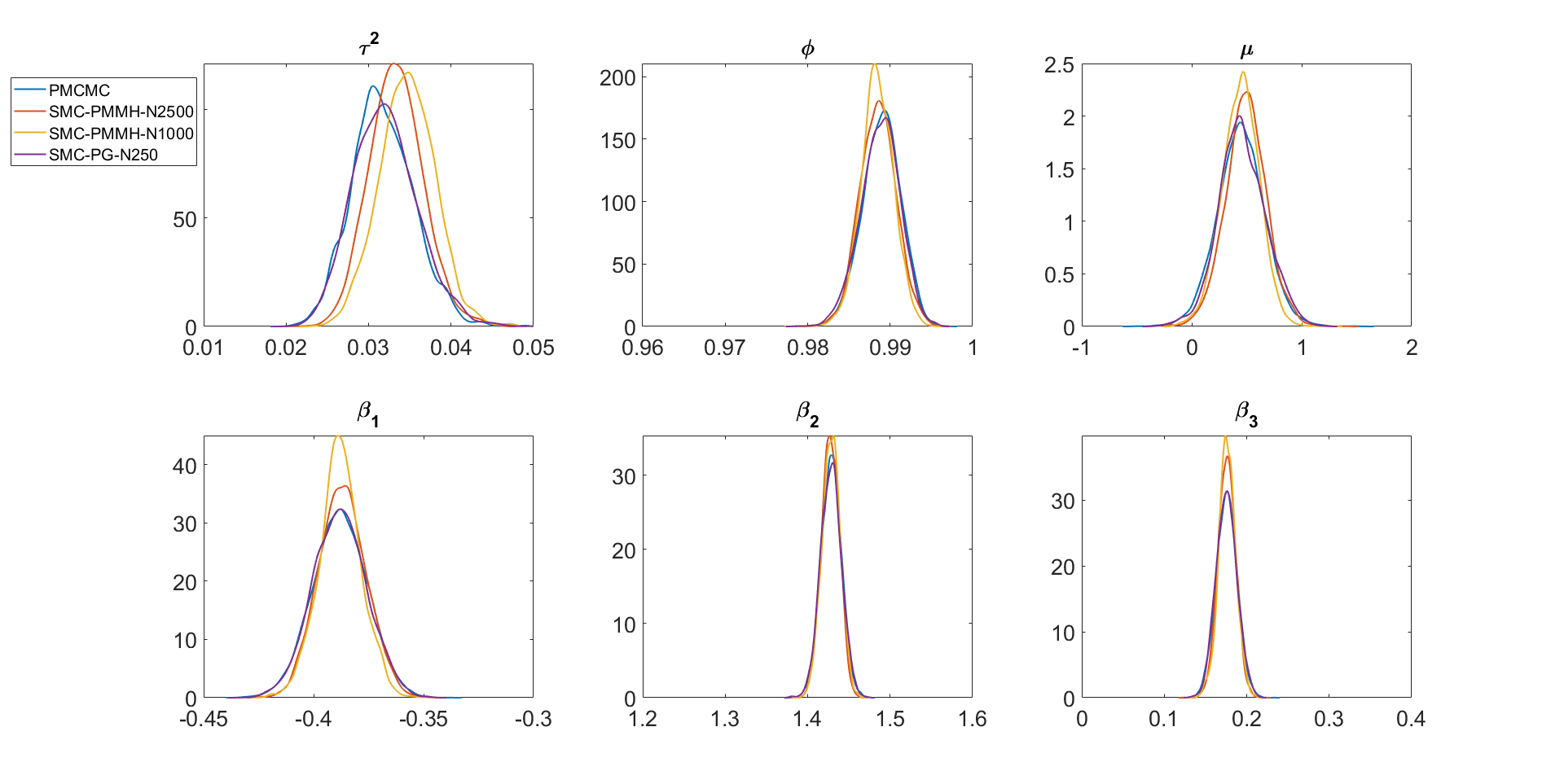
Figure 3: The kernel density estimates of some marginal posterior densities of the univariate SV parameters with the covariate coefficients estimated using the PHS (PMCMC), SMC-PMMH-DF and SMC-PG methods.

4.2 Time Series Diagnostics

The sequential SMC approach in Section 2.2.2 allows us to efficiently estimate the sequence of standard normal random variables used to form the goodness of fit statistics to test for the adequacy of a general time series state space model (Gerlach et al.,, 1998). Let $y_{1},...,y_{T}$ be a sequence of time series observations generated by the continuous random variables $Y_{1},...,Y_{T}$. If the correct model is fitted to the data, then the sequence

$$u_{t}=p\left(Y_{t}\leq y_{t}|\bm{y}_{1:t-1}\right),\;t=1,...,T,$$ (8)

is a realization of independent uniform $U\left(0,1\right)$ random variables. A sequence of independent standard normal random variables $N\left(0,1\right)$ is obtained by setting $v_{t}=\Phi^{-1}\left(u_{t}\right)$, where $\Phi$ is the standard normal cumulative distribution function. To obtain $u_{t}$, it is necessary to integrate out the parameters and the latent states by evaluating

$$u_{t}=\int p\left(Y_{t}\leq y_{t}|\bm{y}_{1:t-1},\bm{\theta},x_{t}\right)p\left(x_{t}|x_{t-1},\bm{\theta}\right)p\left(\bm{\theta},\bm{x}_{1:t-1}|\bm{y}_{1:t-1}\right)d\bm{\theta}\,d{\bm{x}}_{1:t}.$$ (9)

For many statistical models, such as the stochastic volatility model, the integral in Eq. (9) cannot be evaluated analytically. One way to estimate $u_{t}$ is to use MCMC or particle MCMC methods. Given a sample of MCMC draws, $\bm{\theta}_{m}$ and $x_{m,t}$ ($m=1,...,M$), from $p\left(\bm{\theta},\bm{x}_{1:t}|\bm{y}_{1:t-1}\right)$, then

$$\widehat{u}_{t}=\frac{1}{M}\sum_{m=1}^{M}p\left(Y_{t}\leq y_{t}|\bm{y}_{1:t-1},\bm{\theta}_{m},x_{m,t}\right).$$

is an estimate of $u_{t}$. The sequence $\widehat{v}_{t}$ is obtained by setting $\widehat{v}_{t}=\Phi^{-1}\left(\widehat{u}_{t}\right)$ for $t=1,...,T$. However, MCMC can be very time-consuming as it is necessary to repeatedly construct the full Markov chain for each time period $t$; see, e.g., (Gerlach et al.,, 1998). The sequential approach, denoted by SMC-PG-seq, can be used to estimate $u_{t}$ efficiently. If the model is correct, the sequence of $\{u_{t}\}$ is uniform and independent and the sequence of $\{v_{t}\}$ is standard normal and independent. We apply the approach to test for model adequacy using simulated and real data. The simulated data uses the parameter values $\phi=0.98$, $\mu=-0.48$, $\tau^{2}=0.02$, and $T=1000$ observations. A single run of the sequential approach, SMC-PG-seq, with $M=560$ samples is used to obtain the estimate of $\widehat{u}_{t}$ and $\widehat{v}_{t}$, for $t=1,...,T$. Fig. 4 shows the diagnostic plots for the series $\widehat{v}_{t}$ for $t=1,...,T$. The autocorrelation plot in the figure suggests that the $v_{t}$ series is uncorrelated. The QQ-plot suggests the $\widehat{v}_{t}$ series is normal. The Anderson-Darling test (Stephens,, 1974) can also be used to test the null hypothesis that the series $v_{t}$ is normally distributed; the null hypothesis is not rejected at the 5% level of significance (p-value=0.65). This is expected because the dataset is simulated from the SV model. We now apply the methods to a sample of daily US food industry stock returns as in the previous section. Fig. 5 shows the diagnostic plots for the series $\widehat{v}_{t}$ for the real data. The autocorrelation plot in the figure suggests that the $v_{t}$ series is uncorrelated; (2) the quantiles of $\widehat{v}_{t}$ are similar to the quantiles of the standard normal distribution, except in both tails. The Anderson-Darling test for normality of the $v_{t}$ series is rejected at the 5% level of significance (p-value=0.00). We conclude from this result that the standard univariate SV model is inadequate for this series.

This shows the usefulness of the SMC-PG-seq to estimate efficiently the sequence $u_{t}$ used to form the goodness of fit statistics to test for the adequacy of a general time series state space model. Another important advantage of sequential SMC over MCMC is that it provides sequential one-step ahead predictive densities of the log returns, and hence prices; this is particularly useful for financial applications. See Section 10 of the Supplement.

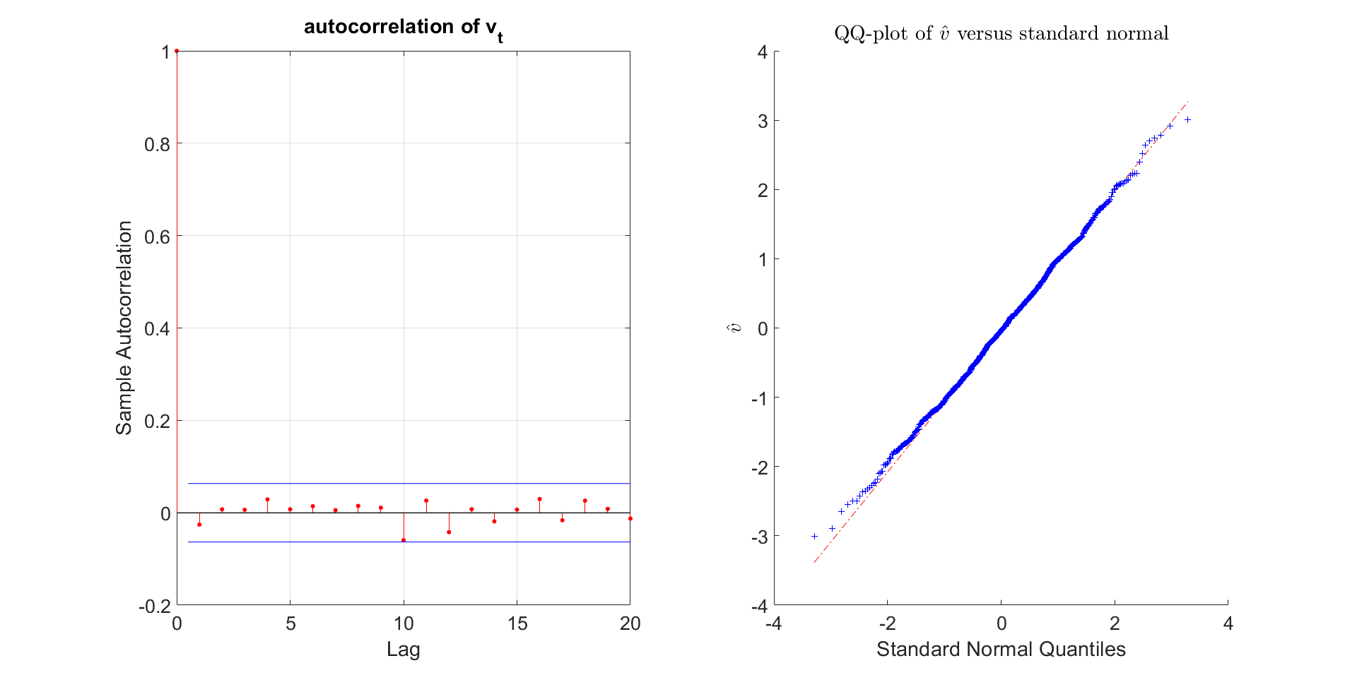
Figure 4: Simulated data, left panel – the autocorrelation plot of the $\widehat{v}_{t}$ series; right panel – the QQ-plot of the $\widehat{v}_{t}$ series versus the standard normal

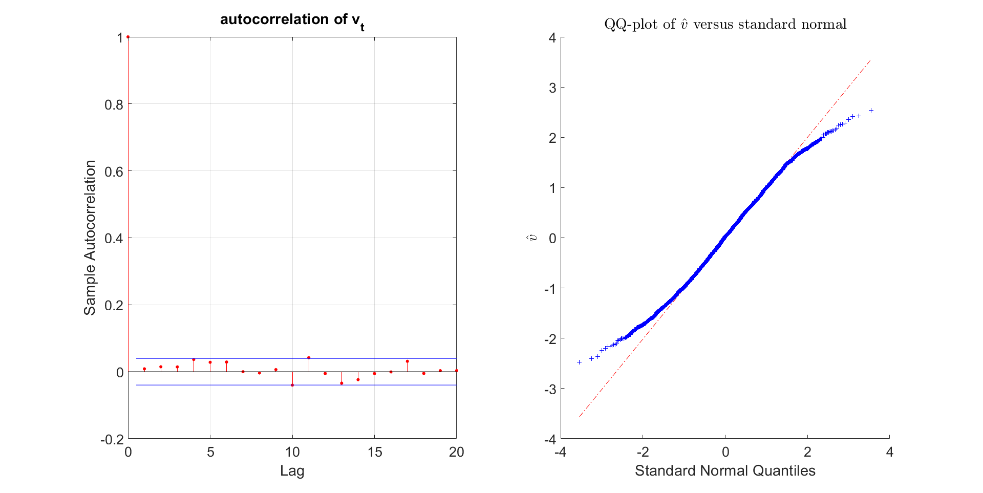
Figure 5: US Food stock returns data, left panel – the autocorrelation plot of the $\widehat{v}_{t}$ series; right panel – the QQ-plot of the $\widehat{v}_{t}$ series versus the standard normal

4.3 SV Model with Outliers

This section uses data simulated from a standard SV model contaminated by outliers to study the performance of the proposed sequential approach SMC-PG-seq with tempering (denoted by SMC-PG-seqT) in Section 2.2.2 and compares it to the standard sequential approach without tempering (denoted by SMC-PG-seqNT). In each scenario, a dataset is generated with $T=1000$ observations using parameter values $\phi=0.98$, $\mu=-0.48$, and $\tau^{2}=0.02$. The generated observations are then contaminated with noise $B_{t}\times\beta_{t}$, where $B_{t}$ is a Bernoulli indicator with parameter $0.01$ and $\beta_{t}$ is normally distributed with mean zero and standard deviation $\kappa$. The parameter $\kappa$ controls the degree of contamination and is set to $\left(5,10,15,25\right)$. A single dataset is simulated in each case. Duan and Fulop, (2015) find that the density tempered SMC method is more robust to outliers than the standard sequential approach because it incorporates the information from the data gradually. We use the estimates of the SMC-PG method as the “gold standard” to assess the accuracy of the sequential SMC-PG-seqT and SMC-PG-seqNT approaches. All the SMC estimates are obtained using 10 independent runs, each with $M=560$ samples. For the SMC-PG and SMC-PG-seqT, $\textrm{ESS}_{\textrm{target}}$ is set to $0.8M$.

Table 3 summarises the simulation results for the SV models with different degrees of data contamination $\kappa=\left(5,10,15,25\right)$. The first three rows report the standard error of the posterior mean estimates of the SV model parameters over the 10 runs of the algorithms; the fourth and fifth rows report the mean and standard error of the log of the marginal likelihood estimates. The SMC-PG-seqT and SMC-PG provide stable results for all values of $\kappa$, but the performance of SMC-PG-seqNT deteriorates as $\kappa$ increases. When $\kappa=25$, the standard error of $\tau^{2}$ from SMC-PG-seqNT is $2.84$ and $2.09$ times larger than from SMC-PG-seqT and SMC-PG, respectively. The Monte Carlo error of the SMC-PG-seqNT increases as outliers become larger in magnitude. The outliers lead to highly variable weights in the reweighting step of the SMC-PG-seqNT algorithm and very low effective sample size (ESS) of the particles. More importantly, the Monte Carlo error of the log of the marginal likelihood estimates seem to deteriorate much faster than the parameter estimates as $\kappa$ increases. When $\kappa=25$, the standard error of the log of the marginal likelihood estimate from SMC-PG-seqNT is 28.05 and 21.49 times larger than from SMC-PG-seqT and SMC-PG, respectively. The log of the marginal likelihood estimates from the PG-seqNT are substantially different to the estimates from SMC-PG-seqT and SMC-PG for $\kappa=10,15,25$. Section 10.1 of the Supplement gives further empirical results. Section 10.2 of the Supplement discusses the flexibility of the SMC-PG-seqT to estimate a two state Markov switching SV model.

Table 3: Simulation results for the SV models with different degrees of data contamination $\kappa=\left(5,10,15,25\right)$. The results are computed from 10 independent runs of each algorithm. The first three rows report the standard error of the posterior mean estimates of the SV parameters $\left(\mu,\phi,\tau^{2}\right)$ over the 10 independent runs. The fourth and fifth rows report the mean and standard error of the log of the marginal likelihood estimates over 10 runs.

	SMC-PG-seqT				SMC-PG-seqNT				SMC-PG
$\kappa$	5	10	15	25	5	10	15	25	5	10	15	25
$\mu$ std err.	0.0100	0.0062	0.0058	0.0048	0.0094	0.0051	0.0081	0.0047	0.0040	0.0026	0.0025	0.0020
$\phi$ std err.	0.0006	0.0023	0.0014	0.0021	0.0007	0.0022	0.0018	0.0039	0.0003	0.0040	0.0010	0.0025
$\tau^{2}$ std err.	0.0011	0.0058	0.0027	0.0069	0.0009	0.0063	0.0034	0.0196	0.0004	0.0087	0.0028	0.0094
$\log\widehat{p}\left(\bm{y}\right)$ mean	-1381.15	-1431.94	-1276.53	-1348.71	-1381.83	-1457.13	-1289.08	-1459.16	-1382.53	-1432.79	-1278.11	-1349.54
$\log\widehat{p}\left(\bm{y}\right)$ std err.	0.3812	0.5907	0.3311	0.5871	0.5808	13.1455	7.2123	16.4654	0.1548	0.3069	0.3321	0.7661

5 The Multivariate Factor Stochastic Volatility Model

5.1 Model

The factor SV model is a parsimonious multivariate stochastic volatility model that is often used to model a vector of stock returns; see, for example, Chib et al., (2006) and Kastner et al., (2017). It is a high dimensional state space model having a large number of parameters and a large number of latent states.

Suppose that $\bm{P}_{t}$ is a $S\times 1$ vector of daily stock prices and define $\bm{y}_{t}\coloneqq\log\bm{P}_{t}-\log\bm{P}_{t-1}$ as the vector of stock returns. We model $\bm{y}_{t}$ as a factor SV model

$$\bm{y}_{t}={\beta}\bm{f}_{t}+{V}_{t}^{\frac{1}{2}}\bm{\epsilon}_{t},\>\left(t=1,...,T\right),$$ (10)

where $\bm{f}_{t}$ is a $K\times 1$ vector of latent factors (with $K\ll S$), and ${\beta}$ is a $S\times K$ factor loading matrix of unknown parameters. The model for the latent factor is $\bm{f}_{t}\sim N\left(0,{D}_{t}\right)$ with $\bm{\epsilon}_{t}\sim N\left(0,I\right)$. The time varying variance matrices ${V}_{t}$ and ${D}_{t}$ depend on the unobserved random variables $\bm{h}_{t}=\left(h_{1t},...,h_{St}\right)$ and $\bm{\lambda}_{t}=\left(\lambda_{1t},...,\lambda_{Kt}\right)$ such that

$${V}_{t}\coloneqq\textrm{diag}\left\{\exp\left(h_{1t}\right),...,\exp\left(h_{St}\right)\right\},\;{D}_{t}:=\textrm{diag}\left\{\exp\left(\lambda_{1t}\right),...,\exp\left(\lambda_{Kt}\right)\right\}.$$

Each of the log-volatilites $\lambda_{kt}$ and $h_{st}$ is assumed to follow an independent first order autoregressive process, with

$$h_{st}-\mu_{\epsilon s}=\phi_{\epsilon s}\left(h_{st-1}-\mu_{\epsilon s}\right)+\eta_{\epsilon st},\quad\eta_{\epsilon st}\sim N\left(0,\tau_{\epsilon s}^{2}\right),\quad s=1,...,S$$ (11)

and

$$\lambda_{kt}=\phi_{fk}\lambda_{kt-1}+\eta_{fkt},\quad\eta_{fkt}\sim N\left(0,\tau_{fk}^{2}\right),\quad k=1,...,K.$$ (12)

For $s=1,...,S$ and $k=1,...,K$, we choose the priors for the persistence parameters $\phi_{\epsilon s}$ and $\phi_{fk}$, the priors $\tau_{\epsilon s}^{2}$, $\tau_{fk}^{2}$, and $\mu_{\epsilon s}$ as in Section 4. For every unrestricted element of the factor loadings matrix ${\beta}$, we follow Kastner et al., (2017) and choose independent Gaussian distributions $N\left(0,1\right)$. These priors cover most possible values in practice.

We also consider the factor stochastic volatility models, where the log-volatilities $h_{s,t}$ follow a continuous time Ornstein-Uhlenbeck (OU) process $\left\{h_{s,t}\right\}_{t\geq 1}$, introduced by Stein and Stein, (1991). The process satisfies,

$$dh_{s,t}=\left\{\alpha_{\epsilon,s}\left(\mu_{\epsilon,s}-h_{s,t}\right)\right\}dt+\tau_{\epsilon,s}dW_{s,t},$$ (13)

where $W_{s,t}$ are independent Wiener processes. Although the continuous time OU diffusion model has a closed form transition density (Brix et al.,, 2018), we investigate the performance of the proposed SMC samplers to estimate state space models using an approximation such as the Euler discretisation.

The Euler scheme can be used as an approximation by placing $M-1$ evenly spaced points between times $t$ and $t+1$. We denote the intermediate volatility components by $h_{s,t,1},...,h_{s,t,M-1}$ and set $h_{s,t,0}=h_{s,t}$ and $h_{s,t,M}=h_{s,t+1}$. The equation for the Euler evolution, starting at $h_{s,t,0}$ is

$$h_{s,t,j+1}|h_{s,t,j}\sim N\left(h_{s,t,j}+\left\{\alpha_{\epsilon,s}\left(\mu_{\epsilon,s}-h_{s,t,j}\right)\right\}\delta,\tau_{\epsilon,s}^{2}\delta\right),$$ (14)

for $j=0,...,M-1$, where $\delta=1/M$. We use the following priors for the OU parameters and assume the parameters are independent apriori: (a) $p\left(\mu_{\epsilon,s}\right)\propto I\left(-10<\mu_{\epsilon,s}<10\right)$, (b) the priors for $\tau^{2}_{\epsilon,s}$ and $\alpha_{\epsilon,s}$ are inverse Gamma $\textrm{IG}\left(v_{0}/2,s_{0}/2\right)$ with $v_{0}=10$ and $s_{0}=1$, for $s=1,...,S$. Section 14 of the Supplement discusses parameterisation and identification issues regarding the factor loading matrix ${\beta}$ and the latent factors $\bm{f}_{t}$.

Conditional Independence in the factor SV model

The key to making the estimation of the factor SV model tractable is that given the values of $\left(\bm{y}_{1:T},\bm{f}_{1:T},{\beta}\right)$, the factor model in Eq. (10) separates into $S+K$ independent components consisting of $K$ univariate SV models for the latent factors with $f_{kt}$ the $t$th ‘observation’ of the $k$th factor univariate SV model and $S$ univariate SV models for the idiosyncratic errors with $\epsilon_{st}$ the $t$th ‘observation’ on the $s$th idiosyncratic error SV model. Section 12 of the Supplement discusses the SMC-HMC, SMC-PG, and SMC-PHS methods for the factor SV model.

5.2 Examples

This section investigates the performance of the SMC samplers to estimate the multivariate factor SV model discussed in Section 5.1 using one factor. A sample of daily returns for $S=26$ value weighted industry portfolios is used, from December 11th, 2001 to 29th November 2005, a total of $1000$ observations. The data is obtained from the Kenneth French website, with the industry portfolios used listed in Section 18 of the Supplement. As in Section 4.1, the PHS is regarded as the “gold standard”; it is run for $50000$ iterates, with another $5000$ iterates used as burn-in.

Our first study discusses how well SMC-PMMH-DF (Duan and Fulop,, 2015) estimates the factor SV model. SMC-PMMH-DF uses the PMMH Markov steps and follows the Pitt et al., (2012) guidelines to set the optimal number of particles in the particle filter to ensure that the variance of the log of the estimated likelihood is around $1$. The PMMH Markov step generates the parameters of the latent factors, with the factor and idiosyncratic log-volatilities “integrated out”, resulting in a $\left(S+K\right)$ dimensional state vector. The tempered measurement density at the $p$th stage is

$$\bigg{\{}N\left(\bm{y}_{t};0,\Sigma_{t}={\beta}D_{t}{\beta}^{{}^{\prime}}+{V}_{t}\right)\bigg{\}}^{a_{p}},$$

Eq. (11) gives the state transition densities for the idiosyncratic log-volatilities ($s=1,\dots,S$) and Eq. (12) gives the state transition equations for the factor log-volatilities ($k=1,\dots,K$).

Table 4 shows the variance of log of the estimated likelihood for different numbers of particles evaluated at posterior means of the parameters obtained using the PHS of Gunawan et al., 2020a with $a_{p}=1$. It shows that even with $5000$ particles, the PMMH Markov step would get stuck. Deligiannidis et al., (2018) proposed the correlated PMMH method and it is possible to implement it in the Markov move step instead of the standard PMMH method of Andrieu et al., (2010).

Table 4: The variance of the log of estimated likelihood for the PMMH step for different numbers of particles for the US stock returns dataset; $T=1000$, $S=26$, and $K=1$ with the tempered sequence $a_{p}$ set to 1, evaluated at the posterior means of the parameters obtained from the PHS of Gunawan et al., 2020a . Time is time in seconds to compute the log of the estimated likelihood once.

Number of Particles	Variance of log of estimated likelihood	Time
250	2198.72	4.86
500	1164.51	9.88
1000	813.53	20.13
2500	439.05	50.43
5000	345.85	99.24

The correlated PMMH correlates the random numbers used in constructing the estimators of the likelihood at current and proposed values of the parameters and sets the correlation very close to 1 to reduce the variance of the difference in the logs of estimated likelihoods at the current and proposed values of the parameters appearing in the Metropolis-Hastings (MH) acceptance ratio. Deligiannidis et al., (2018) show that the correlated PMMH can be much more efficient and can significantly reduce the number of particles required by the standard PMMH approach when the dimension of the latent states is small. However, the current example considers a high dimensional latent state vector in the one factor-Factor SV model. Mendes et al., (2020) found that it is very challenging to preserve the correlation between the logs of the estimated likelihoods for such a high dimensional state space model. The Markov move based on the correlated PMMH approach will also get stuck at lower temperatures unless enough particles are used to ensure the variance of the log of the estimated likelihood is around 1.

A second drawback of the PMMH Markov move step as in Duan and Fulop, (2015) is that the dimension of the parameter space in the factor SV model is large making it very hard to implement the PMMH Markov step efficiently. Section 4.1 shows that SMC-PG is much more efficient than SMC-PMMH-DF for estimating univariate SV model with $50$ covariates. It is difficult to obtain good proposals for the high-dimensional parameters because the first and second derivatives of log of the estimated likelihood with respect to the parameters are unavailable analytically and can only be estimated. Sherlock et al., (2015) note that in general it is even more difficult to obtain accurate estimate of the gradient of the log of the estimated likelihood than it is to obtain accurate estimates of the log of the estimated likelihood. Nemeth et al., (2016) and Mendes et al., (2020) found that the behaviour of particle Metropolis adjusted Langevin Algorithm depends critically on how accurately we can estimate the gradient of the log-posterior. If the variance of the gradient of the log-posterior is insufficiently small, then there is no advantage in using particle MALA over the random walk proposal. Table 4 shows that the variance of the log of the estimated likelihood is still very large, even with $5000$ particles. Therefore, there is no advantage in using particle MALA. The random walk proposal is easy to implement, but it is very inefficient in high dimensions.

The second study compares PHS to the approximate MCMC sampler of Kastner et al., (2017) for estimating the factor SV model. Kastner et al., use the approach proposed by Kim et al., (1998) to approximate the distribution of innovations in the log outcomes by a mixture of normals. Kim et al., correct their approximation by importance sampling, which gives a simulation consistent estimation for the univariate SV model. However, the Kastner et al., estimator is not simulation consistent because it does not correct for these approximations for the factor SV model. The PHS is simulation consistent in the sense that as the number of samples of the parameters $\bm{\theta}$ and latent states $\bm{x}_{1:T}$ tends to infinity, the PHS estimates converge to their true posterior distributions. We implement the MCMC of Kastner et al., using the R package factorstochvol (Hosszejni and Kastner,, 2019), using the default priors in the R package factorstochvol in the comparison. The priors for $\tau^{2}_{\epsilon,s}$ for $s=1,...,S$ and $\tau^{2}_{f,k}$ for $k=1,...,K$ are $G(0.5,1)$ gamma density with shape $0.5$ and scale $1$. The prior for $\mu_{\epsilon,s}$ for $s=1,...,S$ is $N(0,10^{14})$. We use the priors given in Section 5.1 for the other parameters.

Fig. 6 shows the marginal posterior density estimates of the parameters $\mu_{\epsilon,16}$, $\phi_{\epsilon,16}$, and $\tau_{\epsilon,16}$ of the factor SV model using PMCMC (PHS) and the MCMC sampler of Kastner et al.,. The figure shows that the MCMC sampler gives different estimates to PHS. Figures 23 to 26 of Section 19 of the Supplement give results for the other parameters in the factor SV model. The figures show that although some of the parameters estimated using the MCMC Kastner et al., sampler are close to the PHS, some others are quite different. In addition, the Gibbs type MCMC sampler as in Kastner et al., cannot handle the factor SV with the log-volatility following diffusion processes discussed in Section 5.3. It is well known that the Gibbs sampler is inefficient for generating parameters for a diffusion model, in particular the variance parameter (Stramer and Bognar,, 2011).

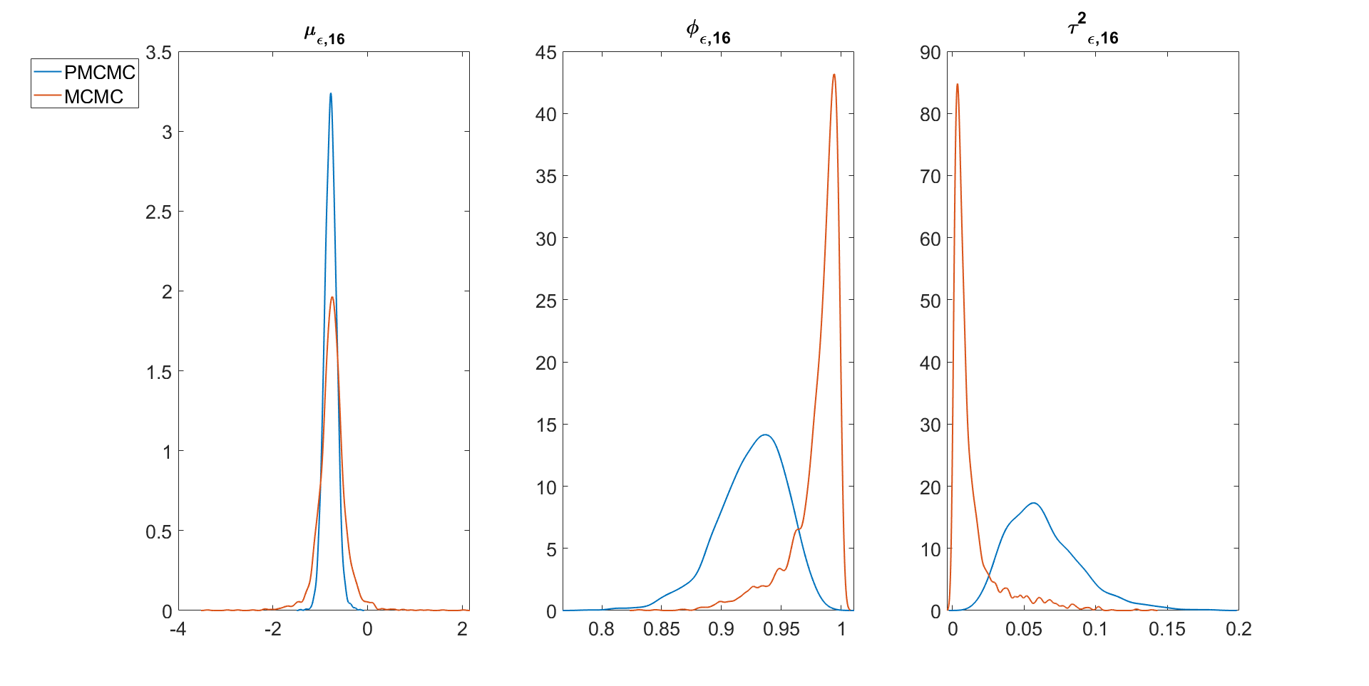
Figure 6: The marginal posterior density plots of the parameters $\mu_{\epsilon,16}$, $\phi_{\epsilon,16}$, and $\tau_{\epsilon,16}$ of the factor SV model estimated using PMCMC (PHS) and the Kastner et al., MCMC.

The third study investigates the performance of the SMC-PG and SMC-PHS methods and compares them to the PHS. The SMC estimates are obtained using 10 independent runs with $M=280$ samples to generate a total of $2800$ samples for each algorithm. For the SMC methods, $\textrm{ESS}_{\textrm{target}}=0.8M$. The computation is done using a Matlab implementation of the algorithms and 28 CPU-cores of a high performance computer cluster.

We use the following notation: $\textrm{SMC-PG}\left(\theta\right)$ means sampling $\theta$ using the SMC-PG method; $\textrm{SMC-PHS}\left(\theta_{1};\theta_{2}\right)$ means sampling $\theta_{1}$ in the PMMH step in Part 1 of Algorithm 5 and $\theta_{2}$ in the PG step. The strategy for the SMC-PHS method is to generate parameters that are subject to slow convergence using a PMMH step and the rest of the parameters are generated conditional on the states using PG steps. We first run the particle Gibbs (PMCMC) sampling algorithm for all the parameters to identify which parameters have convergence issues. We then generate these parameters in the PMMH step in SMC-PHS algorithm. Gunawan et al., 2020a find that the particle Gibbs sampler usually generates the variance parameters in the state transition equation inefficiently, i.e., $\tau^{2}_{\epsilon,s}$ for $s=1,...,S$ and $\tau^{2}_{f,k}$ for $k=1,...,K$. We compare the following methods: (I) the SMC-PHS $\left(\bm{\tau}_{\epsilon}^{2},\bm{\tau}_{f}^{2};\bm{\mu}_{\epsilon},\bm{\phi}_{\epsilon},\bm{\phi}_{f},\bm{f}_{1:T},\bm{\beta}\right)$, (II) the $\textrm{SMC-PG}\left(\bm{\tau}_{\epsilon}^{2},\bm{\tau}_{f}^{2},\bm{\mu}_{\epsilon},\bm{\phi}_{\epsilon},\bm{\phi}_{f},f_{1:T},\bm{\beta}\right)$, (III) PHS $\left(\bm{\tau}_{\epsilon}^{2},\bm{\tau}_{f}^{2};\bm{\phi}_{f},\bm{f}_{1:T},\bm{\beta},\bm{\mu}_{\epsilon},\bm{\phi}_{\epsilon}\right)$.

Fig. 7 plots the marginal posterior density estimates of the parameters $\mu_{\epsilon,16}$, $\phi_{\epsilon,16}$, and $\tau_{\epsilon,16}$ of the factor SV model estimated using PMCMC (PHS), SMC-PG and SMC-PHS. The figure shows that the SMC-PG and SMC-PHS methods give the same estimates as PHS, with SMC-PG slightly more accurate at estimating $\mu_{\epsilon,16}$. Figures 19 to 22 in the Supplement show all the other parameters of the factor SV model. In general, the SMC-PG and SMC-PHS estimates are very close to the PHS estimates for all parameters. Table 5 shows the estimates of the log of the marginal likelihood for the one factor model estimated using the SMC-PHS and SMC-PG methods. The table shows that the estimated standard errors of the estimates of the log of the marginal likelihood estimated using SMC-PHS are 1.87 times bigger than for the SMC-PG methods. The standard errors can be reduced by increasing the number of SMC samples $M$ and setting the $\textrm{ESS}_{\textrm{target}}>0.8M$. The table also shows that the number of annealing steps of SMC-PG and SMC-PHS methods are comparable. The Markov move based on the PHS is computationally more expensive than the Markov move based on PG only because it is necessary to run the particle filter twice at each iteration.

We now compare the predictive performance of the SMC-PG and SMC-PHS methods with the (exact) PHS. The minimum variance portfolio implied by the $h$ step-ahead time-varying covariance matrix $\Sigma_{T+h}$, is considered; it can be used to uniquely define the optimal portfolio weights (Bodnar et al.,, 2017),

$$w_{port,T+h}:=\frac{\Sigma_{T+h}^{-1}\mathbb{1}}{\mathbb{1}^{\top}\Sigma_{T+h}^{-1}\mathbb{1}},$$

where $\mathbb{1}$ denotes an S-variate vector of ones. The optimal portfolio weights give the lowest possible risk for a given expected portfolio return.

Figure 8 shows the multiple-step ahead predictive densities $\widehat{p}\left({y}_{T+h}|\bm{y}_{1:T}\right)$ of an optimally weighted combination of all series, for $h=1,...,10$ obtained using SMC-PG, SMC-PHS, and PHS. The figure shows that the predictive densities obtained using SMC-PG method are very close to the exact predictive densities obtained from the PHS. The predictive densities obtained using SMC-PHS are slightly less accurate. Section 19 of the Supplement give additional empirical results for the factor SV model.

This example suggests that: (a) the PMMH Markov move is expensive for the factor SV model, as it requires the number of particles to be greater than $5000$; (b) the PMMH Markov move is unsuitable for the factor SV model because the dimension of the parameter space in the factor SV model is large; (c) the approximate MCMC method of Kastner et al., can give unreliable estimates for some parameters in the factor SV model; (d) for the standard factor SV model, SMC-PG is faster and slightly more accurate than SMC-PHS in estimating the posterior densities of the factor SV parameters and the predictive densities.

Table 5: Factor SV model estimated using PHS, SMC-PG, and SMC-PHS for the US returns data with $T=1000$, $S=26$, and $K=1$. Time is in minutes for one run of the algorithm. The table gives: (i) the estimates of the log of the marginal likelihood $\textrm{log}\widehat{p}\left(\bm{y}_{1:T}\right)$ based on the average of the 10 runs, and the standard error of the estimate (in brackets). (ii) the average value of the number of annealing steps $P$ averaged over the 10 runs

Method	N	R	P	Time	$\textrm{log}\widehat{p}\left(\bm{y}_{1:T}\right)$
SMC-PG	250	10	289	2307.38	$\underset{\left(30.29\right)}{-26149.66}$
SMC-PHS	250	10	274	6003.34	$\underset{\left(56.55\right)}{-26176.99}$

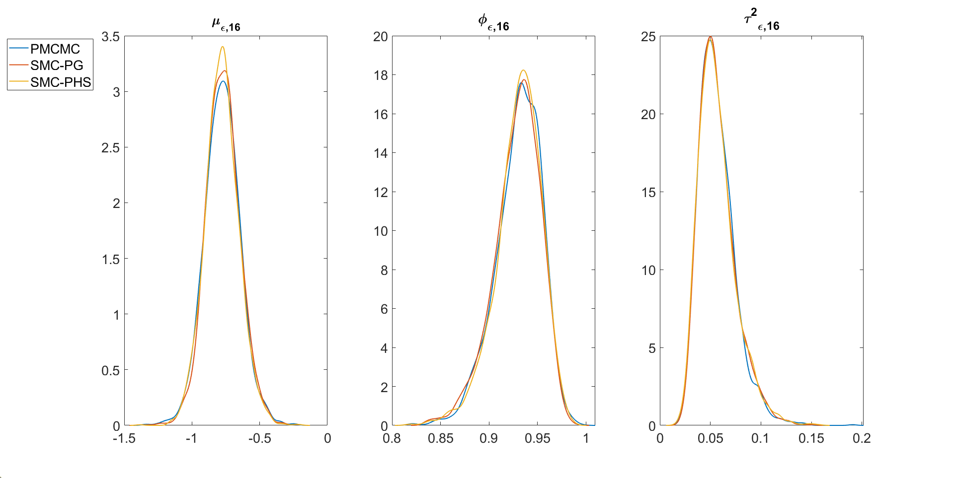
Figure 7: The marginal posterior density plots of the parameters $\mu_{\epsilon,16}$, $\phi_{\epsilon,16}$, and $\tau_{\epsilon,16}$ of the factor SV model estimated using PMCMC (PHS), SMC-PG, and SMC-PHS.

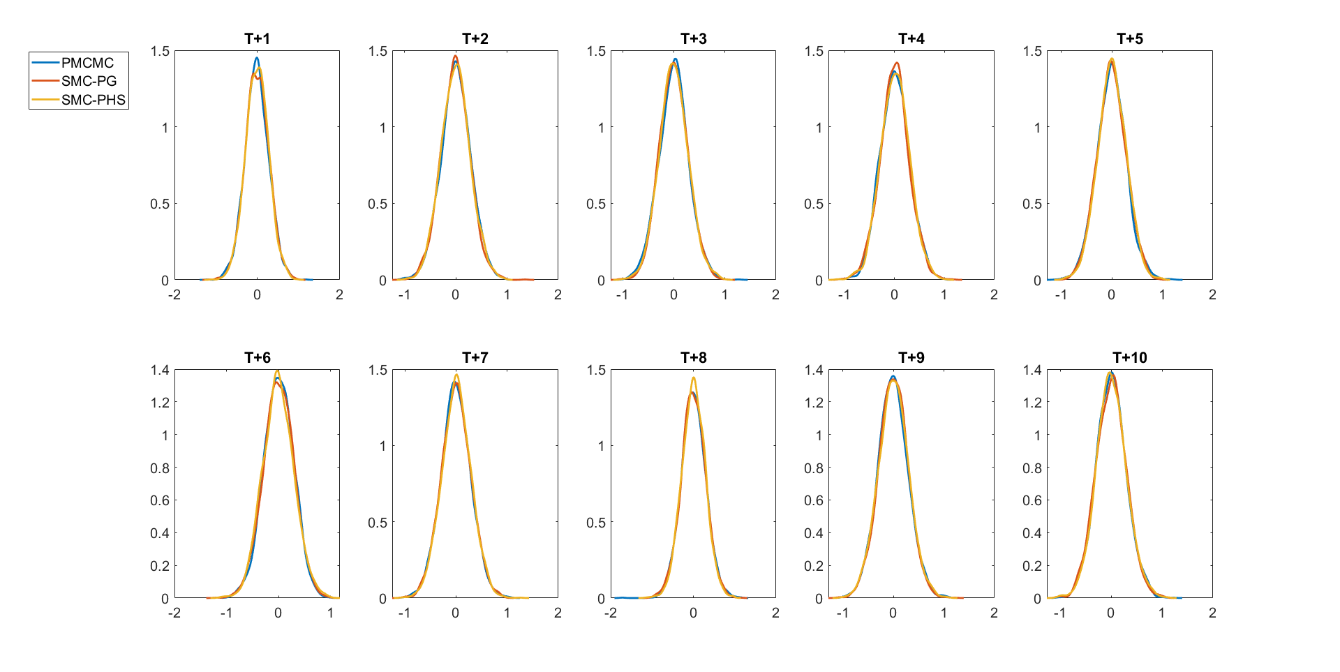
Figure 8: Plot of the predictive densities $\widehat{p}(y_{T+h}|y_{1:T})$ of an optimally weighted portfolio, for $h=1,...,10$, estimated using PMCMC (PHS), SMC-PG, and SMC-PHS.

5.3 Factor SV Model with the Ornstein-Uhlenbeck Diffusion Processes

This section considers the factor stochastic volatility model, where the log-volatilities of the factors follow a standard SV model and the idiosyncratic log-volatilities follow a continuous time Ornstein-Uhlenbeck (OU) process $\left\{h_{s,t}\right\}_{t\geq 1}$ (Stein and Stein,, 1991). Although the continuous time OU diffusion model has a closed form transition density (Brix et al.,, 2018), this section investigates the performance of SMC-PG and SMC-PHS when estimating the state space model using an approximation such as the Euler discretisation. For this example, we use the first $S=10$ daily portfolio returns listed in Section 18 of the Supplement, from December 11th, 2001 to 29th November 2005, a total of $1000$ observations.

Fig. 9 shows the trace plots of the parameters $\bm{\tau}_{\epsilon}$, $\bm{\alpha}_{\epsilon}$, and $\bm{\mu}_{\epsilon}$ of the factor SV model, where the idiosyncratic log-volatilities follow OU processes and the factor log-volatilities follow the standard SV model estimated using particle Gibbs. The figure shows that the posterior draws of $\bm{\tau}^{2}_{\epsilon}$ and $\bm{\alpha}_{\epsilon}$ are highly autocorrelated and fail to converge. We estimate all the OU parameters in the PMMH steps in PHS and SMC-PHS. We compare the following samplers: (I) the SMC-PHS $\left(\bm{\tau}_{\epsilon}^{2},\bm{\tau}_{f}^{2},\bm{\mu}_{\epsilon},\bm{\alpha}_{\epsilon};\bm{\phi}_{f},\bm{f}_{1:T},\beta\right)$, (II) the $\textrm{SMC-PG}\left(\bm{\tau}_{\epsilon}^{2},\bm{\tau}_{f}^{2},\bm{\mu}_{\epsilon},\bm{\alpha}_{\epsilon},\bm{\phi}_{f},\bm{f}_{1:T},\beta\right)$, (III) PHS $\left(\bm{\tau}_{\epsilon}^{2},\bm{\tau}_{f}^{2},\bm{\mu}_{\epsilon},\bm{\alpha}_{\epsilon};\bm{\phi}_{f},\bm{f}_{1:T},\beta\right)$, and (IV) the $\textrm{PG}\left(\bm{\tau}_{\epsilon}^{2},\bm{\tau}_{f}^{2},\bm{\mu}_{\epsilon},\bm{\alpha}_{\epsilon},\bm{\phi}_{f},\bm{f}_{1:T},\beta\right)$. The PG and PHS are run for 20000 iterates with another 5000 iterates used as burn-in.

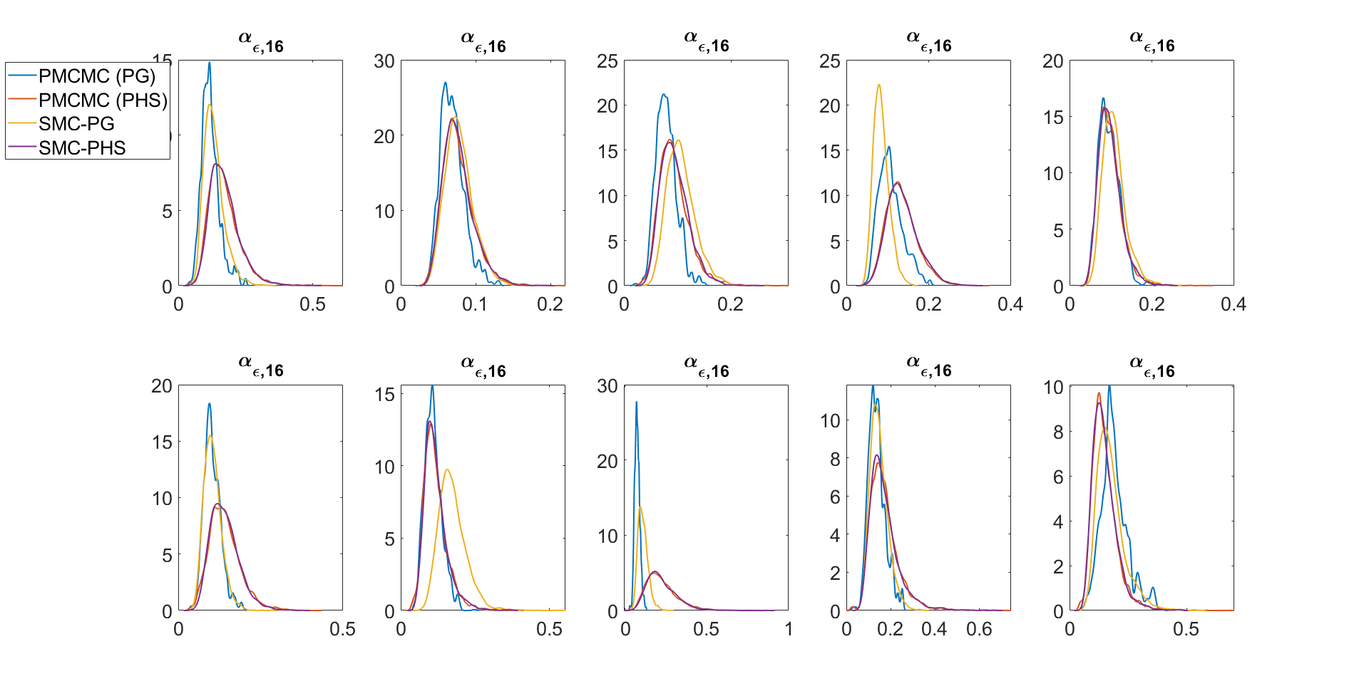
Figure 27: The marginal posterior density plots of the $\bm{\alpha}_{\epsilon}$ of the factor SV model, where the idiosyncratic errors follow OU processed estimated using PHS, PG, SMC-PG, and SMC-PHS.

Fig. 10 shows the marginal posterior density plots of the parameters $\tau^{2}_{\epsilon}$ of the factor SV models, where the idiosyncratic errors follow OU processes estimated using the PHS, PG, SMC-PG, and SMC-PHS methods. The figure shows that the PG and SMC-PG estimates are very different to PHS. SMC-PHS gives the same estimates as PHS. Similar observations hold for the parameters $\bm{\alpha}_{\epsilon}$ in Fig. 27 of Section 19 of the Supplement. This example suggests that: (a) The SMC-PG estimates for the model parameters are unreliable and are highly correlated with the states. (b) The SMC-PHS estimates are accurate as they generate the parameters that are highly correlated with the states using PMMH steps, and the other parameters are generated using PG steps.

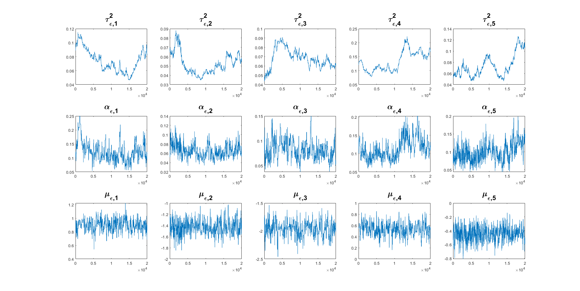
Figure 9: Trace plots of the parameters $\bm{\tau}_{\epsilon}$, $\bm{\alpha}_{\epsilon}$, and $\bm{\mu}_{\epsilon}$ of the factor SV model, where the idiosyncratic errors follow the OU process estimated using particle Gibbs.

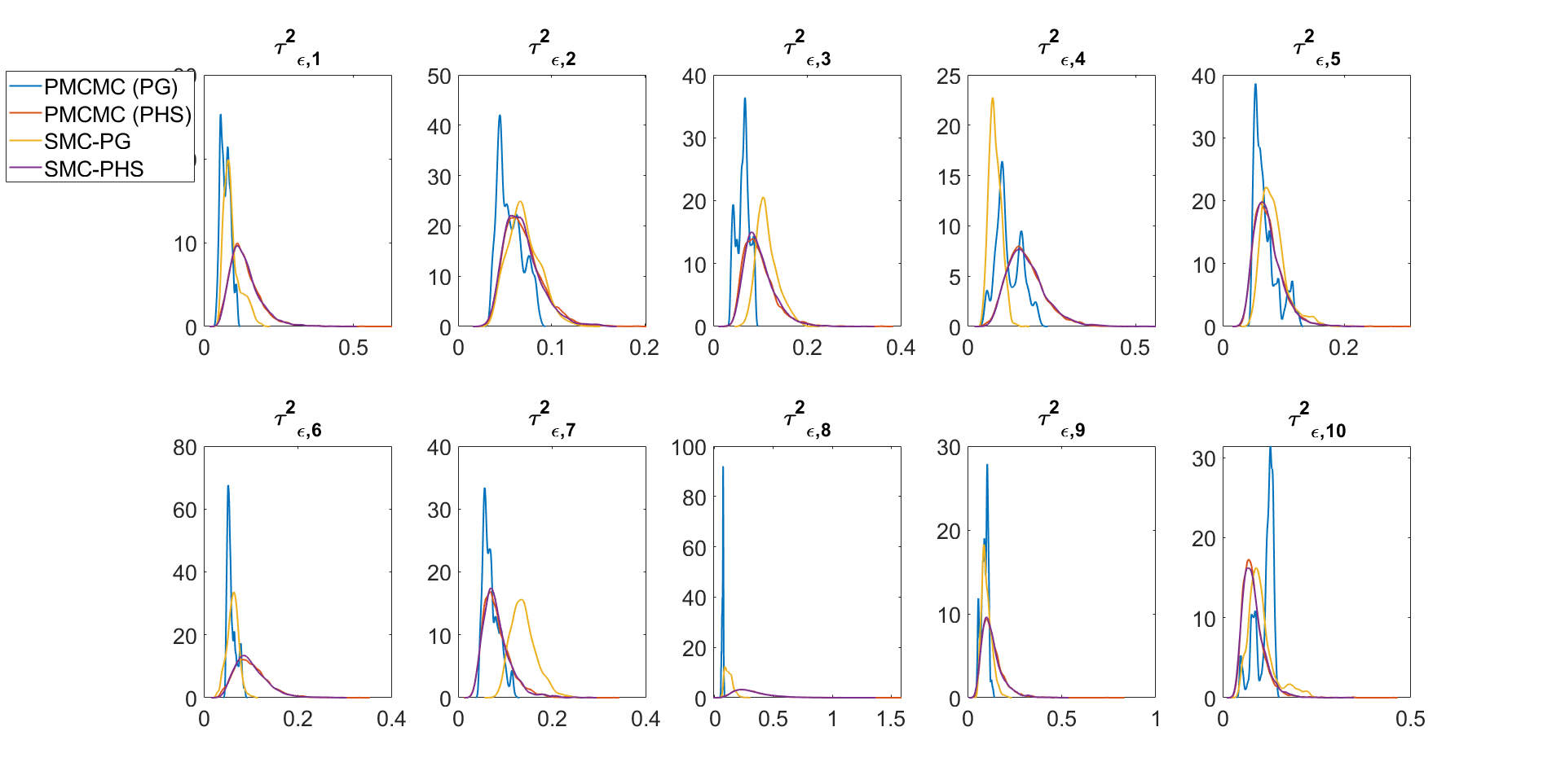
Figure 10: The marginal posterior density estimates of the parameters $\bm{\tau}_{\epsilon}$ of the factor SV models, where the idiosyncratic errors follow the OU process estimated using PHS, PG, SMC-PG, and SMC-PHS.

6 Conclusions

The paper proposes flexible SMC approaches that can be used for both batch and sequential state and parameter estimation problems, and which also lead to accurate one-step and multiple-step ahead predictions. The approaches are based on Markov move steps that are more efficient than in previous SMC approaches in Duan and Fulop, (2015), Fulop and Li, (2013), and Chopin et al., (2013). We show that the methods work well for both simulated and real data and can handle higher-dimensional states and parameters than previously possible by current SMC approaches. The data analyses suggest that (a) SMC-PG gives parameter and states estimates close to PHS for both univariate and standard factor SV models. It also accurately estimates the predictive densities of individual stock returns and the minimum variance portfolio. (b) SMC-PG gives inaccurate parameter estimates for $\bm{\alpha}_{\epsilon}$ and $\bm{\tau}^{2}_{\epsilon}$ for the factor SV model with the idiosyncratic log-volatilities following OU processes. This is because the OU parameters, in particular, the $\bm{\alpha}_{\epsilon}$ and $\bm{\tau}^{2}_{\epsilon}$ are highly correlated with the states. (c) SMC-PHS provides flexible Markov move steps, where the parameters that are highly correlated with the states are generated by PMMH and all other parameters are generated by PG steps conditioning on the states. Section 5.3 shows that the SMC-PHS gives accurate estimates for the OU parameters. (d) The SMC-PMMH-DF of Duan and Fulop, (2015) cannot handle state space models with a large number of parameters and states. Section 5.2 gives further details. (e) The MCMC sampler of Kastner et al., (2017) gives similar results to the PHS for most of the factor SV parameters, but some parameter estimates are different. The Gibbs type MCMC sampler as in Kastner et al., (2017) cannot handle the factor SV with the log-volatility following diffusion processes. (f) The sequential SMC approach allows us to efficiently estimate the sequence of standard normal random variables used to form the goodness of fit statistics to test for the adequacy of a general time series state space model. (g) The sequential approach with tempering provides joint sequential inference for states and parameters and is more robust than the sequential approach without tempering.

7 Acknowledgement

We thank the AE and the four reviewers for their comments which improved both the presentation and the technical content of the paper.

8 Supplementary Material

This article has an online supplement that contains additional technical details and empirical results.

Online Supplement: Robust Particle Density Tempering for State Space Models

We use the following notation in the supplement. Eq. (1), Alg. 1, and Sampling Scheme 1, etc, refer to the main paper, while Eq. (S1), Alg. S1, and Sampling Scheme S1, etc, refer to the supplement.

9 Markov move steps for the univariate SV model

9.1 Sampling the latent volatilities using Hamiltonian Monte Carlo

For the univariate SV model Eq. (1), we need the gradient of the log-likelihood $\nabla_{\bm{x}}\mathcal{L}\left(\bm{x}\right)$ with respect to each of the latent volatilities. The required gradient for $t=1$ is

$$\nabla_{x_{1}}\mathcal{L}\left(\bm{x}\right)=a_{p}\left(-0.5+0.5y_{1}^{2}\exp\left(-x_{1}\right)\right)-\frac{\left(1-\phi^{2}\right)}{\tau^{2}}\left(x_{1}-\mu\right)+\frac{\phi}{\tau^{2}}\left(x_{2}-\mu-\phi\left(x_{1}-\mu\right)\right);$$

the gradient for $1<t<T$ is

$$\nabla_{x_{t}}\mathcal{L}\left(\bm{x}\right) =a_{p}\left(-0.5+0.5y_{t}^{2}\exp\left(-x_{t}\right)\right)+\frac{\phi}{\tau^{2}}\left(x_{t+1}-\mu-\phi\left(x_{t}-\mu\right)\right)-$$

$$\frac{1}{\tau^{2}}\left(x_{t}-\mu-\phi\left(x_{t-1}-\mu\right)\right);$$

and, for $t=T$, the gradient is

$$\nabla_{x_{T}}\mathcal{L}\left(\bm{x}\right) =a_{p}\left(-0.5+0.5y_{T}^{2}\exp\left(-x_{T}\right)\right)-\frac{1}{\tau^{2}}\left(x_{T}-\mu-\phi\left(x_{T-1}-\mu\right)\right).$$

9.2 Sampling the Univariate SV parameters

For $i=1,...,M$, we sample $\mu_{i}|\bm{x}_{i1:T},\bm{y}_{1:T},\bm{\theta}_{-\mu}$ from $N\left(\mu_{\mu},\sigma_{\mu}^{2}\right)$ truncated to $\left(-10,10\right)$, where

$$\sigma_{\mu}^{2}=\frac{\tau_{i}^{2}}{1-\phi_{i}^{2}+\left(T-1\right)\left(1-\phi_{i}\right)^{2}}$$

and

$$\mu_{\mu}=\dfrac{\sigma_{\mu}^{2}}{\tau_{i}^{2}}\left(x_{i1}\left(1-\phi_{i}^{2}\right)+\sum_{t=2}^{T}x_{it}-\phi_{i}x_{it}+\phi_{i}^{2}x_{it-1}-\phi_{i}x_{it-1}\right).$$

We sample the persistence parameter $\phi_{i}$ by drawing a proposed value $\phi_{i}^{*}$ from $N\left(\mu_{\phi},\sigma_{\phi}^{2}\right)$ truncated within $\left(-1,1\right)$, where

$$\sigma_{\phi}^{2}=\frac{\tau_{i}^{2}}{\sum_{t=2}^{T}\left(x_{it-1}-\mu_{i}\right)^{2}-\left(x_{i1}-\mu_{i}\right)^{2}}$$

and

$$\mu_{\phi}=\sigma_{\phi}^{2}\frac{\sum_{t=2}^{T}\left(x_{it}-\mu_{i}\right)\left(x_{it-1}-\mu_{i}\right)}{\tau_{i}^{2}},$$

and accept with probability

$$\min\left(1,\frac{p\left(\phi_{i}^{*}\right)\sqrt{1-\phi_{i}^{2*}}}{p\left(\phi_{i}\right)\sqrt{1-\phi_{i}^{2}}}\right).$$

We sample $\tau_{i}^{2}$ from $\textrm{IG}\left(v_{1}/2,s_{1}/2\right)$, where $v_{1}=v_{0}+T$ and $s_{1}=s_{0}+\left(1-\phi_{i}^{2}\right)\left(x_{i1}-\mu_{i}\right)^{2}+\sum_{t=2}^{T}\left(x_{it}-\mu_{i}-\phi_{i}\left(x_{it-1}-\mu_{i}\right)\right)^{2}$.

10 Additional Results for univariate SV models

The terms SMC-PG, SMC-PG-seq, and SMC-PG-batch-seq for SMC-PG denote batch estimation, sequential estimation, and a combination of batch and sequential estimation, respectively. For the SMC-PG-batch-seq method, batch estimation is used for the first 80% of the data and sequential estimation is used for the rest.

Fig. 11 presents the sequential parameter learning in the univariate SV model estimated using SMC-PG-seq. Clearly, all parameter estimates vary a lot at the start when the number of observations is small, then stabilise as the number of observations gets larger. This sequential approach can take into account impacts of parameter and model uncertainties on decision-making over time.

Another important advantage of SMC-PG-batch-seq is that it provides sequential one-step and multi-step ahead predictive densities of the future observations $y_{T+h},h>0$.

Fig. 12 shows the sequential one-step ahead predictive density for log-return of the US food industry from 22/06/2011 to 11/11/2013 estimated using the SMC-PG-batch-seq method. Financial risk measures such as value at risk (VaR) can be computed from the one step ahead predictive densities. The VaR is the most widely used measure of market risk (Holton,, 2003). The $t$-period $\pi$-VaR of a return series, denoted as $\textrm{VaR}_{\pi,t}$, is defined by

$$\pi:=\Pr\left(y_{t}\leq\textrm{VaR}_{\pi,t}|{\cal F}_{t-1}\right),$$

where ${\cal F}_{t-1}$ is the information available to time $t-1$. The one-step ahead $\pi\%$-VaR, $\textrm{VaR}_{\pi,t+1}$, can be estimated using the $\pi$th-quantile of the posterior predictive return distribution at time $t+1$ given the information up to time $t$. Fig. 13 shows the sequential one-step ahead VaR estimates at risk levels $0.01$, $0.05$, and $0.10$ for the log return of the US food industry from 22/06/2011 to 11/11/2013. The lowest VaR estimates are between 08/08/2011 to 18/08/2011 obtained using the SMC-PG-batch-seq method.

Figure 14 shows that the SMC-PG estimates are very close to the PHS estimates for all the covariate coefficients. The SMC-PMMH-DF based estimates differ from the PHS estimates even with $N=2500$ particles. SMC-PMMH-DF uses a PMMH approach with random walk proposal for the parameters in the Markov move component. The random walk is easy to implement, but is not efficient for high-dimensional parameters.

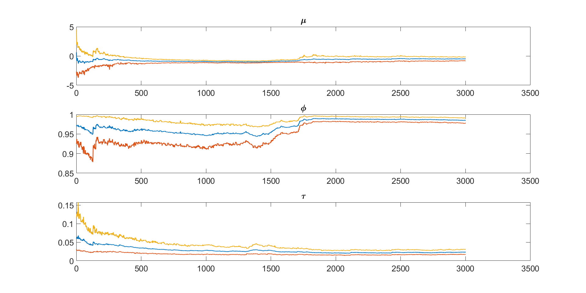
Figure 11: The evolution over time of the posterior mean estimates of the parameters $\mu$, $\phi$, and $\tau^{2}$ (with 95% Bayesian credible intervals) for the univariate SV Model estimated using SMC-PG-seq.

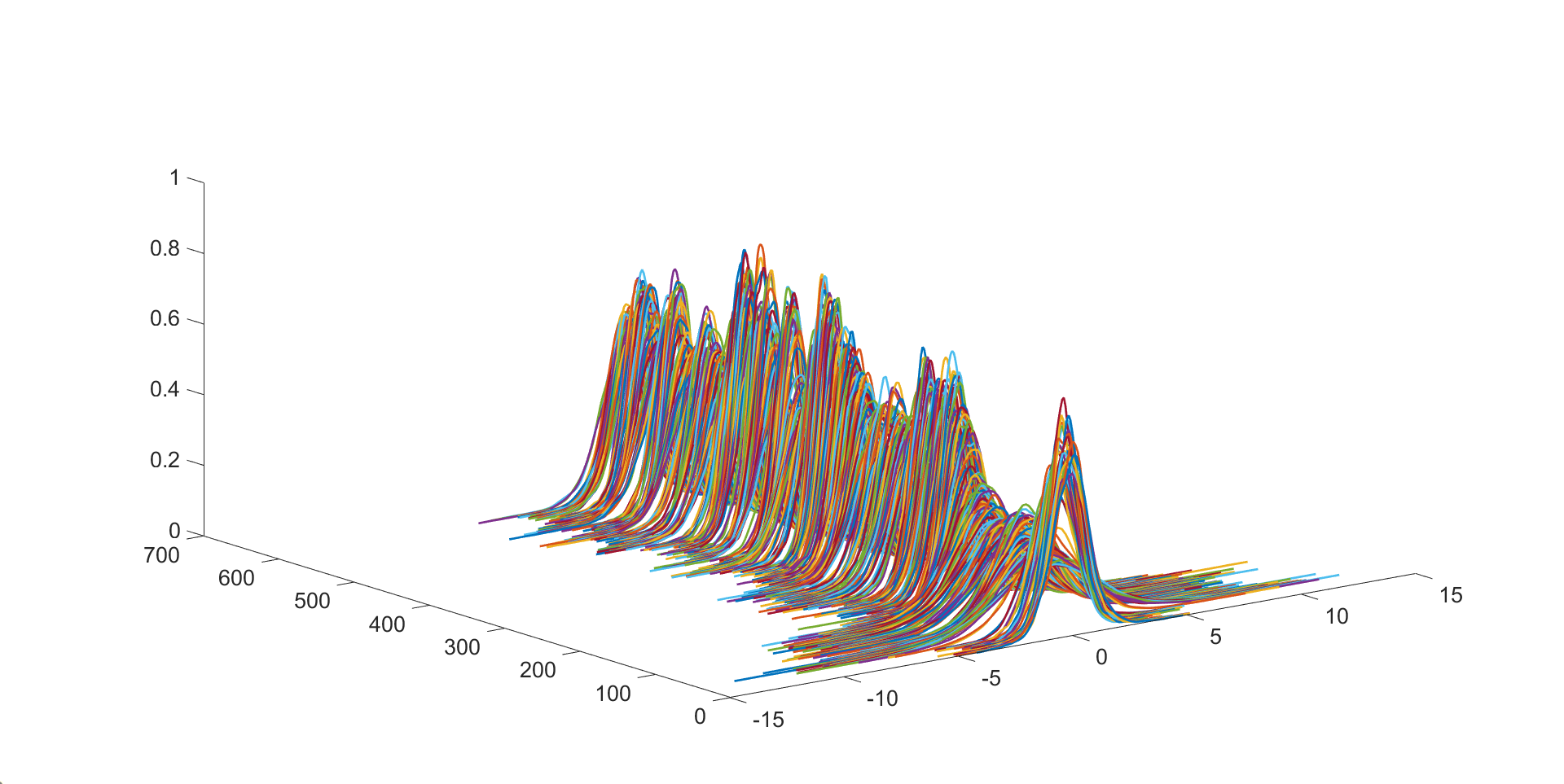
Figure 12: Sequential one-step ahead predictive density estimates for log return of the US food industry from 22/06/2011 to 11/11/2013 estimated using the SMC-PG-batch-seq method

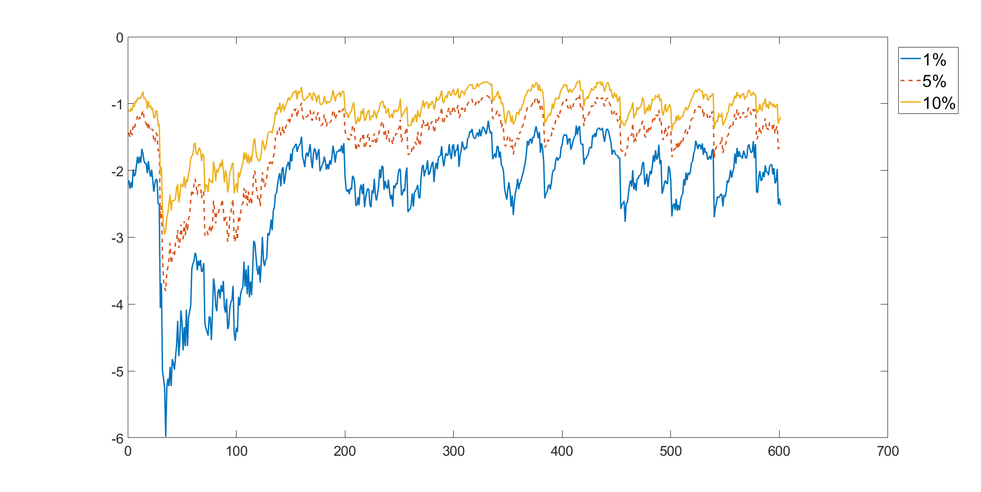
Figure 13: Sequential one-step ahead Value at Risk (VaR) estimates for log return of the US food industry from 22/06/2011 to 11/11/2013 estimated using the SMC-PG-batch-seq method

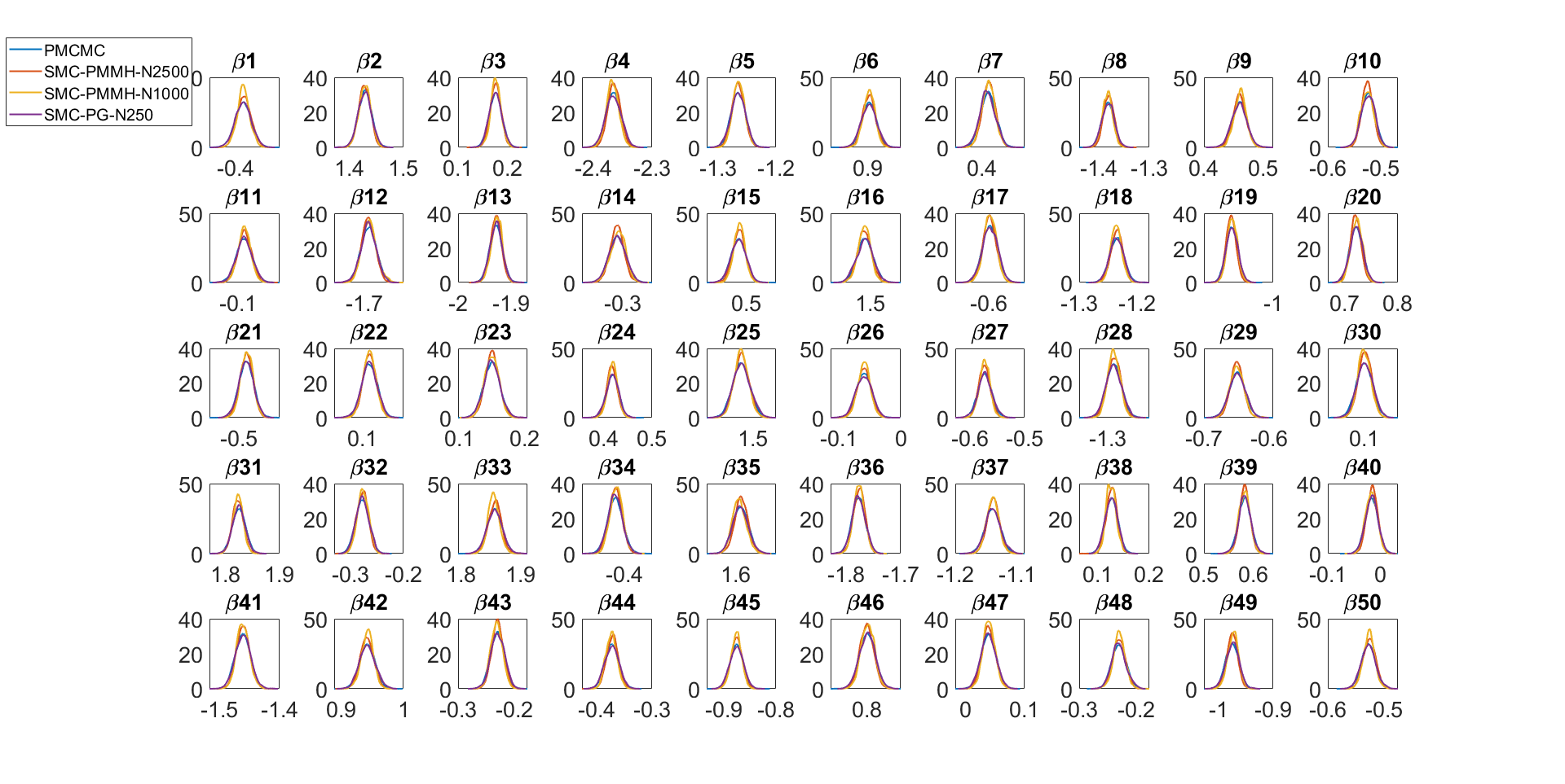
Figure 14: The kernel density estimates of the marginal posterior densities of the $\beta$ parameters of the univariate SV model with the covariate coefficients estimated using PHS with $N=100$, SMC-PMMH-DF with $N=2500$, and SMC-PG methods with $N=250$

10.1 Additional results for the SV model with outliers

Fig. 15 shows the normalised ESS over time obtained from a run of SMC-PG-seqNT for the SV model with $\kappa=25$. The normalised ESS is close to zero when the data point is the outlier. This suggests that SMC-PG-seqT is more stable than the SMC-PG-seqNT, as it ensures the ESS stays close to $\textrm{ESS}_{\textrm{target}}$. Fig. 16 (top panel) shows the number of Markov steps over time obtained from a run of SMC-PG-seqT algorithm.

The top panel of Fig. 16 shows that a larger number of Markov move steps are taken when the data is an outlier. The middle panel of Fig. 16 shows the absolute value of the log of $\widehat{p}\left(y_{t}|\bm{y}_{1:t-1}\right)$ for $t=1,..,T$. This figure can be used to identify outliers in the data by investigating the unusually large absolute value of the log of $\widehat{p}\left(y_{t}|\bm{y}_{1:t-1}\right)$ for $t=1,...,T$.

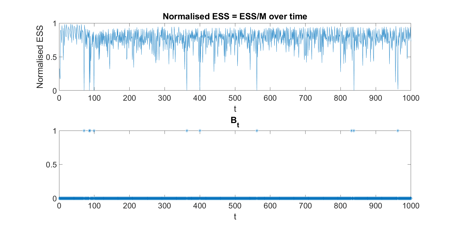
Figure 15: Top panel: The normalised ESS $\left(ESS/M\right)$ over time obtained from a run of SMC-PG-seqNT algorithm for SV model with $\kappa=25$; Bottom panel: The series $B_{t}$ for $t=1,...,T;$ $B_{t}=1$ if the observation is an outlier and $0$, otherwise.

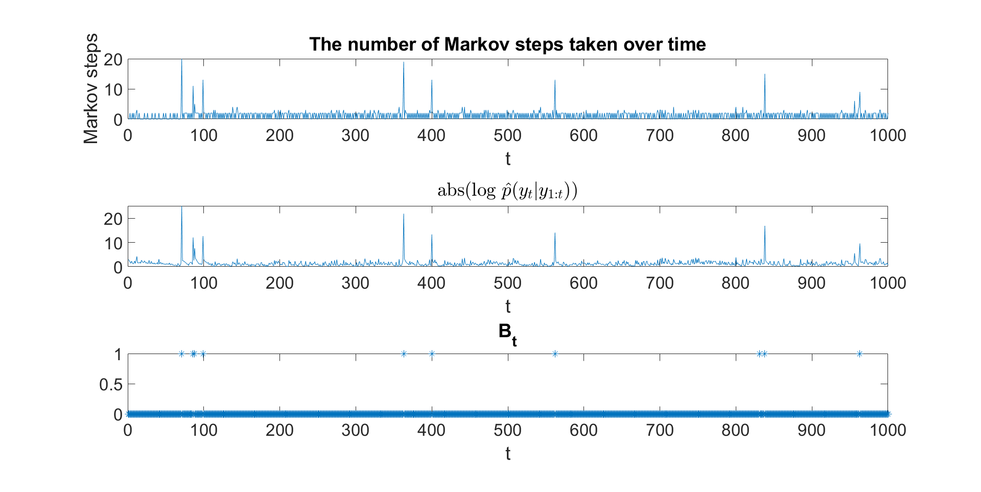
Figure 16: Top panel: The number of annealing steps $P$ over time obtained from a run of SMC-PG-seqT for the SV model with $\kappa=25$; Middle panel: the absolute value of the log of $\widehat{p}\left(y_{t}|\bm{y}_{1:t-1}\right)$ for $t=1,..,T$; Bottom panel: The $B_{t}$, $t=1,...,T$ series; $B_{t}=1$ if the observation is an outlier and $0$ otherwise.

10.2 Markov Switching Stochastic Volatility Models

This section demonstrates the flexibility of SMC-PG-seqT by applying it to the two state Markov switching SV model

$$y_{t}=\mu_{s_{t}}^{p}+\exp\left(x_{t}/2\right)\epsilon_{t},\;x_{t}=\mu+\phi\left(x_{t-1}-\mu\right)+\tau\eta_{t},\;x_{1}\sim N\left(\mu,\tau^{2}/\left(1-\phi^{2}\right)\right);$$

$\epsilon_{t}\sim N\left(0,1\right)$, $\eta_{t}\sim N\left(0,1\right)$, $\bm{s}_{1:T}=\left(s_{1},...,s_{T}\right)^{\intercal}$, $s_{t}=1,2$ and $s_{t}=k$ indicates that $y_{t}$ is from regime $k$. This model is similar to that in Chib, (1998).

The one-step ahead transition probability matrix for $s_{t}$ is

$$P=\left[\begin{array}[]{cc}p_{11}&p_{12}\\ p_{21}&p_{22}\end{array}\right],$$

where $p_{lk}=\Pr\left(s_{t}=k|s_{t-1}=l\right)$ is the probability of moving from regime $l$ at time $t-1$ to regime $k$ at time $t$. The prior for $\mu^{p}_{1}$ and $\mu^{p}_{2}$ is $N\left(0,100\right)$; the prior $p_{11}$ and $p_{22}$ is $Beta\left(4,1\right)$. The same priors as in Section 4 are used for the other SV parameters.

We compare the performance of SMC-PG-seqT to SMC-PG-seqNT and SMC-PG for this model. A dataset is generated with $T=1000$ observations using parameter values $\phi=0.98$, $\mu=-0.48$, $\tau^{2}=0.02$, $\mu_{1}=-1$, $\mu_{2}=1$, and $p_{kk}=0.99$ for $k=1,2$. The SMC-PG method is used as the “gold standard” to assess the accuracy of the SMC-PG-seqT and SMC-PG-seqNT. All the SMC estimates are obtained using 10 independent runs, each with $M=560$ samples. For the SMC-PG and SMC-PG-seqT, the $\textrm{ESS}_{\textrm{target}}$ is set to $0.8M$.

Table 6 summarizes the simulation results for the Markov switching SV model. The first seven rows report the standard errors of the posterior mean estimates of the model parameters over the 10 runs; the eighth and ninth rows report the mean and standard error of the log of the marginal likelihood estimates. In general, the standard error of the posterior mean estimates obtained by SMC-PG-seqT and SMC-PG is smaller than SMC-PG-seqNT. The standard error of the log of the marginal likelihood estimates from PG-seqNT is about 3 times larger than from SMC-PG-seqT and SMC-PG. Fig. 17 shows the normalised ESS over time obtained from a run of PG-seqNT algorithm. Clearly, the normalised ESS is quite small when the state changes from 1 to 2 or from 2 to 1.

Table 6: Simulation results for the Markov switching SV models. The results are computed from 10 independent runs of each algorithm. The first seven rows report the standard error of the posterior mean estimates of the SV parameters $\left(\mu_{1}^{p},\mu_{2}^{p},\mu,\phi,\tau^{2}\right)$ over the 10 independent runs. The eighth and ninth rows report the mean and standard error of the log of the marginal likelihood estimates over 10 runs.

	SMC-PG-seqT	SMC-PG-seqNT	SMC-PG
$\mu_{1}^{p}$ std err.	0.0013	0.0013	0.0008
$\mu_{2}^{p}$ std err.	0.0015	0.0025	0.0013
$p_{11}$ std err.	0.0003	0.0003	0.0001
$p_{22}$ std err.	0.0004	0.0002	0.0003
$\mu$ std err.	0.0084	0.0066	0.0033
$\phi$ std err.	0.0007	0.0008	0.0004
$\tau^{2}$ std err.	0.0005	0.0005	0.0005
$\log\widehat{p}\left(\bm{y}\right)$ mean	$-1434.83$	$-1435.20$	$-1437.83$
$\log\widehat{p}\left(\bm{y}\right)$ std err.	0.5100	1.5235	0.5071

Figure 17: Top panel: The normalised $ESS:=\left(ESS/M\right)$ over time obtained from the SMC-PG-seqNT algorithm for the Markov switching SV model; Bottom panel: the true series $s_{t}$ for $t=1,...,T$

11 Augmented Target Density for SMC-PG

Similarly to Andrieu et al., (2010), the SMC-PG constructs a sequence of tempered densities $\xi_{a_{p}}\left(\bm{\theta},\bm{x}_{1:T}\right)$, $p=1,...,P$, based on the following augmented target density

$$\widetilde{\xi}_{a_{p}}\left(\bm{x}_{1:T}^{\bm{j}_{1:T}},\bm{j}_{1:T},\bm{U}_{1:T}^{-\bm{j}_{1:T}},\bm{\theta}\right)=\frac{\xi_{a_{p}}\left(\bm{\theta},\bm{x}_{1:T}^{\bm{j}_{1:T}}\right)}{N^{T}}$$ (15)

$$\times\frac{\psi\left(\bm{U}_{1:T}|\bm{\theta}\right)}{m_{1}\left({x}_{1}^{j_{1}}|\bm{\theta},{y}_{1}\right)\prod_{t=2}^{T}\widetilde{W}_{t-1}^{\widetilde{b}_{t-1}^{j_{t}}}m_{t}\left({x}_{t}^{j_{t}}|{x}_{t-1}^{\widetilde{b}_{t-1}^{j_{t}}},\bm{\theta},{y}_{t}\right)}.$$

The next lemma shows that the marginal distribution of the augmented target distribution in Eq. (15) is proportional to the joint tempered posterior density of the parameters and states $\xi_{a_{p}}\left(\bm{\theta},\bm{x}_{1:T}\right)$

Lemma 1.

The target distribution in Eq. (15) has the marginal distribution

$$\widetilde{\xi}_{a_{p}}\left(\bm{x}_{1:T}^{\bm{j}_{1:T}},\bm{j}_{1:T},\bm{\theta}\right)=N^{-T}\xi_{a_{p}}\left(\bm{\theta},\bm{x}_{1:T}^{\bm{j}_{1:T}}\right).$$

Proof.

We prove the lemma by carrying out the marginalisation similarly to the proof in Andrieu et al., (2010) for particle Gibbs MCMC. The marginal distribution $\xi_{a_{p}}\left(\bm{x}_{1:T}^{\bm{j}_{1:T}},\bm{j}_{1:T},\bm{\theta}\right)$ is obtained by integrating $\widetilde{\xi}_{a_{p}}\left(\bm{x}_{1:T}^{\bm{j}_{1:T}},\bm{j}_{1:T},\bm{U}_{1:T}^{-\bm{j}_{1:T}},\bm{\theta}\right)$ over $\left(\bm{x}_{1:T}^{\left(-\bm{j}_{1:T}\right)},\widetilde{\bm{b}}_{1:T-1}\right)$. We begin by integrating over $\left(\bm{x}_{T}^{-j_{T}},\bm{\widetilde{b}}_{T-1}\right)$ to obtain

$$\widetilde{\xi}_{a_{p}}\left(d\bm{x}_{1:T}^{\bm{j}_{1:T}},\bm{j}_{1:T},d\bm{x}_{1:T-1}^{\left(-\bm{j}_{1:T-1}\right)},d\widetilde{\bm{b}}_{1:T-2},d\bm{\theta}\right)=\frac{\xi_{a_{p}}\left(d\bm{\theta},d\bm{x}_{1:T}^{\bm{j}_{1:T}}\right)}{N^{T}}$$ (16)

$$\frac{\psi\left(d\bm{x}_{1:T-1}^{1:N},d\widetilde{\bm{b}}_{1:T-2}|\bm{\theta}\right)}{m_{1}\left(d\bm{x}_{1}^{j_{1}}|\bm{\theta},\bm{y}_{1}\right)\prod_{t=2}^{T-1}\widetilde{W}_{t-1}^{\widetilde{b}_{t-1}^{j_{t}}}m_{t}\left(d\bm{x}_{t}^{j_{t}}|\bm{x}_{t-1}^{\widetilde{b}_{t-1}^{j_{t}}},\bm{\theta}\right)}.$$

We repeat this for $t=T-2,...,2$, to obtain,

$$\widetilde{\xi}_{a_{p}}\left(d\bm{x}_{1}^{\left(-j_{1}\right)},d\bm{x}_{1:T}^{\bm{j}_{1:T}},\bm{j}_{1:T},d\bm{\theta}\right)=\frac{\xi_{a_{p}}\left(d\bm{\theta},d\bm{x}_{1:T}^{\bm{j}_{1:T}}\right)}{N^{T}}\times\frac{\psi\left(d\bm{x}_{1}^{1:N}\right)}{m_{1}\left(d\bm{x}_{1}^{j_{1}}|\bm{\theta},\bm{y}_{1}\right)}.$$

Finally, we integrate over $\bm{x}_{1}^{j_{1}}$, to obtain

$$\widetilde{\xi}_{a_{p}}\left(d\bm{x}_{1:T}^{\bm{j}_{1:T}},\bm{j}_{1:T},d\bm{\theta}\right)=\frac{\xi_{a_{p}}\left(d\bm{\theta},d\bm{x}_{1:T}^{\bm{j}_{1:T}}\right)}{N^{T}}.$$

∎

12 Augmented Intermediate Target Density for the Factor SV model

This section provides the augmented tempered target density for the factor SV model; It includes all the random variables produced by the $S+K$ univariate particle filter methods that generate the factor log-volatilities $\bm{\lambda}_{k,1:T}$, for $k=1,...,K$, and the idiosyncratic log-volatilities $\bm{h}_{s,1:T}$ for $s=1,...,S$, as well as the latent factors $\bm{f}_{1:T}$ and the parameters $\bm{\theta}$. Eq. (11) specifies the particle filters for the idiosyncratic SV log-volatilities $\bm{h}_{s,1:T}$ for $s=1,...,S$, and Eq. (12) specifies the univariate particle filters that generate the factor log-volatilities $\bm{\lambda}_{k,1:T}$, for $k=1,...,K$. The $N$ weighted samples at time $t$ for the factor log-volatilities are denoted by $\left(\bm{\lambda}_{kt}^{1:N},\widetilde{\bm{W}}_{fkt}^{1:N}\right)$ and the idiosyncratic error log-volatilities by $\left(\bm{h}_{st}^{1:N},\widetilde{\bm{W}}_{\epsilon st}^{1:N}\right)$. The corresponding proposal densities are $m_{fk1}\left(\lambda_{k1}|\bm{\theta}_{fk},\bm{y}_{1}\right)$, $m_{fkt}\left(\lambda_{kt}|\lambda_{kt-1},\bm{\theta}_{fk},\bm{y}_{t}\right)$, $m_{\epsilon s1}\left(h_{s1}|\bm{\theta}_{\epsilon s},\bm{y}_{1}\right)$, and $m_{\epsilon st}\left(h_{st}|h_{st-1},\bm{\theta}_{\epsilon s},\bm{y}_{t}\right)$ for the $t=2,...,T$. The resampling schemes are denoted by ${\cal M}\left(\widetilde{\bm{b}}_{\epsilon st-1}^{1:N}|\widetilde{\bm{W}}_{\epsilon st-1}^{1:N}\right)$, where each $\widetilde{b}_{\epsilon st-1}^{j}=k$ indexes a particle in $\left(\bm{h}_{st-1}^{1:N},\widetilde{\bm{W}}_{\epsilon st-1}^{1:N}\right)$ and is chosen with probability $\widetilde{W}_{\epsilon st-1}^{k}$; ${\cal M}\left(\widetilde{\bm{b}}_{fkt-1}^{1:N}|\widetilde{\bm{W}}_{fkt-1}^{1:N}\right)$ is defined similarly.

The vectors of particles are denoted as

$$\bm{U}_{\epsilon s,1:T}\coloneqq\left(\bm{h}_{s1}^{1:N},...,\bm{h}_{sT}^{1:N},\widetilde{\bm{b}}_{\epsilon s1}^{1:N},...,\widetilde{\bm{b}}_{\epsilon sT-1}^{1:N}\right)$$

and

$$\bm{U}_{fk,1:T}\coloneqq\left(\bm{\lambda}_{k1}^{1:N},...,\bm{\lambda}_{kT}^{1:N},\widetilde{\bm{b}}_{fk1}^{1:N},...,\widetilde{\bm{b}}_{fkT-1}^{1:N}\right).$$

The joint distribution of the particles given the parameters is

$$\psi_{\epsilon s}\left(\bm{U}_{\epsilon s,1:T}^{1:N}|\bm{\theta}_{\epsilon s}\right)\coloneqq\\ \prod_{j=1}^{N}m_{\epsilon s1}\left(h_{s1}^{j}|\bm{y}_{1},\bm{\theta}_{\epsilon s}\right)\prod_{t=2}^{T}\left\{{\cal M}\left(\widetilde{\bm{b}}_{\epsilon st-1}^{1:N}|\widetilde{\bm{W}}_{\epsilon st-1}^{1:N}\right)\prod_{j=1}^{N}m_{\epsilon st}\left(h_{st}^{j}|h_{st-1}^{\widetilde{{b}}_{\epsilon st-1}^{j}},\bm{\theta}_{\epsilon s},\bm{y}_{t}\right)\right\},$$

for $s=1,...,S$ and

$$\psi_{fk}\left(\bm{U}_{fk,1:T}^{1:N}|\bm{\theta}_{fk}\right)\coloneqq\\ \prod_{j=1}^{N}m_{fk1}\left(\lambda_{k1}^{j}|\bm{y}_{1},\bm{\theta}_{fk}\right)\prod_{t=2}^{T}\left\{{\cal M}\left(\widetilde{\bm{b}}_{fkt-1}^{1:N}|\widetilde{\bm{W}}_{fkt-1}^{1:N}\right)\prod_{j=1}^{N}m_{fkt}\left(\lambda_{kt}^{j}|\lambda_{kt-1}^{\widetilde{{b}}_{fkt-1}^{j}},\bm{\theta}_{fk},\bm{y}_{t}\right)\right\},$$

for $k=1,...,K$.

Next, we define indices $\bm{j}_{\epsilon s,1:T}$ for $s=1,...,S$, the selected particle trajectory $\bm{h}_{s,1:T}^{\bm{j}_{\epsilon s,1:T}}=\left(h_{s1}^{j_{\epsilon s1}},...,h_{sT}^{j_{\epsilon sT}}\right)$, indices $\bm{j}_{fk,1:T}$ for $k=1,...,K$ and the selected particle trajectory $\bm{\lambda}_{k,1:T}^{\bm{j}_{fk,1:T}}=\left(\lambda_{k1}^{j_{fk1}},...,\lambda_{kT}^{j_{fkT}}\right)$.

The augmented intermediate target density in this case consists of all the particle filter variables

$$\tilde{\xi}_{a_{p}}\left(\bm{U}_{\epsilon s,1:T},\bm{U}_{fk,1:T},\bm{\theta},\bm{f}_{1:T}\right)\coloneqq\frac{\xi_{a_{p}}\left(d\bm{\theta},d\bm{h}_{1:T}^{\bm{j}_{\epsilon s,1:T}},d\bm{\lambda}_{1:T}^{\bm{j}_{fk,1:T}},d\bm{f}_{1:T}\right)}{N^{T\left(S+K\right)}}\times$$ (17)

$$\prod_{s=1}^{S}\frac{\psi_{\epsilon s}\left(\bm{U}_{\epsilon s,1:T}|\bm{\theta}_{\epsilon s}\right)}{m_{\epsilon s1}\left(h_{s1}^{j_{\epsilon s1}}|\bm{\theta}_{\epsilon s}\right)\prod_{t=2}^{T}\widetilde{W}_{\epsilon st-1}^{\widetilde{b}_{\epsilon st-1}^{j_{\epsilon st}}}m_{\epsilon st}\left(h_{st}^{j_{\epsilon st}}|h_{st-1}^{\widetilde{b}_{\epsilon st-1}^{j_{\epsilon st}}},\bm{\theta}_{\epsilon s}\right)}$$

$$\prod_{k=1}^{K}\frac{\psi_{fk}\left(\bm{U}_{fk,1:T}|\bm{\theta}_{fk}\right)}{m_{fk1}\left(\lambda_{k1}^{j_{fk1}}|\bm{\theta}_{fk}\right)\prod_{t=2}^{T}\widetilde{W}_{fkt-1}^{\widetilde{b}_{fkt-1}^{j_{fkt}}}m_{fkt}\left(\lambda_{kt}^{j_{fkt}}|\lambda_{kt-1}^{\widetilde{b}_{fkt-1}^{j_{fkt}}},\bm{\theta}_{fk}\right)}.$$

The next lemma shows that the target distribution in Eq. (17) has the required marginal distribution. Mendes et al., (2020) give a similar lemma and proof for describing the augmented target density of the factor SV models for PMCMC methods.

Lemma 2.

The target distribution in Eq. (17) has the marginal distribution

$$\tilde{\xi}_{a_{p}}\left(\bm{h}_{1:T}^{\bm{j}_{\epsilon s,1:T}},\bm{j}_{\epsilon s,1:T},\bm{\lambda}_{1:T}^{\bm{j}_{fk,1:T}},\bm{j}_{fk,1:T},\bm{\theta},\bm{f}_{1:T}\right)=\frac{\xi_{a_{p}}\left(d\bm{\theta},d\bm{h}_{1:T}^{\bm{j}_{\epsilon s,1:T}},d\bm{\lambda}_{1:T}^{\bm{j}_{fk,1:T}},d\bm{f}_{1:T}\right)}{N^{T\left(S+K\right)}}.$$

Proof.

Similarly to the proof of Lemma 1, we can show that the marginal distribution

$$\tilde{\xi}_{a_{p}}\left(d\bm{h}_{1:T}^{\bm{j}_{\epsilon s,1:T}},\bm{j}_{\epsilon s,1:T},d\bm{\lambda}_{1:T}^{\bm{j}_{fk,1:T}},\bm{j}_{fk,1:T},d\bm{\theta},d\bm{f}_{1:T}\right)=\frac{\xi_{a_{p}}\left(d\bm{\theta},d\bm{h}_{1:T}^{\bm{j}_{\epsilon s,1:T}},d\bm{\lambda}_{1:T}^{\bm{j}_{fk,1:T}},d\bm{f}_{1:T}\right)}{N^{T\left(S+K\right)}},$$

is obtained by integrating $\tilde{\xi}_{a_{p}}\left(\bm{U}_{\epsilon s,1:T},\bm{U}_{fk,1:T},\bm{\theta},\bm{f}_{1:T}\right)$ over $\left(\bm{h}_{s1:T}^{\left(-\bm{j}_{\epsilon s1:T}\right)},\widetilde{\bm{b}}_{\epsilon s1:T-1}\right)$ for $s=1,...,S$, and $\left(\bm{\lambda}_{k1:T}^{\left(-\bm{j}_{fk1:T}\right)},\widetilde{\bm{b}}_{fk1:T-1}\right)$ for $k=1,...,K$. ∎

12.1 Application of the SMC-HMC method to the Multivariate Factor Stochastic Volatility Model

This section discusses the application of the SMC-HMC method to the multivariate factor SV model described in Section 5.1 in a batch context. We first define the appropriate sequence of intermediate target densities,

$$\xi_{a_{p}}\left(\bm{\theta},\bm{h}_{1:T},\bm{\lambda}_{1:T},\bm{f}_{1:T}\right) \propto p\left(\bm{y}_{1:T}|\bm{f}_{1:T},\bm{h}_{1:T},\bm{\lambda}_{1:T},\bm{\theta}\right)^{a_{p}}p\left(\bm{f}_{1:T}|\bm{h}_{1:T},\bm{\lambda}_{1:T},\bm{\theta}\right)$$ (18)

$$\times p\left(\bm{\lambda}_{1:T},\bm{h}_{1:T}|\bm{\theta}\right)p\left(\bm{\theta}\right),$$

$$\text{where}\quad\bm{\theta} =\left\{\bm{\theta}_{\epsilon s}=\left\{\mu_{\epsilon s},\phi_{\epsilon s},\tau_{\epsilon s}^{2}\right\}_{s=1}^{S},{\bm{\theta}}_{fk}=\left\{\phi_{fk},\tau_{fk}^{2}\right\}_{k=1}^{K},{\beta}\right\},$$

$$p\left(\bm{y}_{1:T}|\bm{f}_{1:T},\bm{h}_{1:T},\bm{\lambda}_{1:T},\bm{\theta}\right)^{a_{p}} =\prod_{t=1}^{T}\prod_{s=1}^{S}p\left(y_{st}|\bm{\beta}_{s},\bm{f}_{t},h_{st}\right)^{a_{p}},$$

$$p\left(\bm{f}_{1:T}|\bm{\lambda}_{1:T}\right) =\prod_{t=1}^{T}\prod_{k=1}^{K}p\left(f_{kt}|\lambda_{kt}\right),$$

$$p\left(\bm{\lambda}_{1:T}|\bm{\theta}_{f}\right) =\prod_{k=1}^{K}\prod_{t=2}^{T}p\left(\lambda_{kt}|\lambda_{kt-1},\bm{\theta}_{fk}\right)p\left(\lambda_{k1}|\bm{\theta}_{fk}\right),$$

$$p\left(\bm{h}_{1:T}|\bm{\theta}_{\epsilon}\right) =\prod_{s=1}^{S}\prod_{t=2}^{T}p\left(h_{st}|h_{st-1},\bm{\theta}_{\epsilon s}\right)p\left(h_{s1}|\bm{\theta}_{\epsilon s}\right).$$

Algorithm 6 gives the Markov move step based on Hamiltonian Monte Carlo for the multivariate factor SV model with the target densities $\xi_{a_{p}}\left(\bm{\theta},\bm{h}_{1:T},\bm{\lambda}_{1:T},\bm{f}_{1:T}\right)$. Steps 1 to 4 update the idiosyncratic log-volatilities parameters $(\mu_{\epsilon s},\phi_{\epsilon s},\tau^{2}_{\epsilon s})$ for $s=1,...,S$, factor log-volatilities parameters $(\phi_{fk},\tau^{2}_{fk})$ for $k=1,...,K$, the factor loading matrix $\beta$ and the latent factors $\bm{f}_{t}$, respectively. Section 13.2 discusses updating the idiosyncratic and factor log-volatilities parameters. Section 14 discusses sampling of the factor loading matrix ${\beta}$ and the latent factors $\bm{f}_{t}$ . Steps 5 and 6 update $S$ idiosyncratic log-volatilities, $\bm{h}_{s,1:T}$ and $K$ factor log-volatilities $\bm{\lambda}_{k,1:T}$ using Hamiltonian Monte Carlo, respectively. Section 13.1 presents the details on updating the idiosyncratic and factor log-volatilities.

Algorithm 6 Markov moves based on Hamiltonian Monte Carlo for multivariate factor SV model

for each $i=1,...,M$,

1. for $s=1:S$

   1. Sample $\mu_{i,\epsilon s}|\bm{h}_{is,1:T},\bm{\theta}_{i,-\mu_{i,\epsilon s}}$

   2. Sample $\phi_{i,\epsilon s}|\bm{h}_{is,1:T},\bm{\theta}_{i,-\phi_{i,\epsilon s}}$

   3. Sample $\tau_{i,\epsilon s}^{2}|\bm{h}_{is,1:T},\bm{\theta}_{i,-\tau_{i,\epsilon s}^{2}}$

2. For $k=1,...,K$

   1. Sample $\phi_{i,fk}|\bm{\lambda}_{ik,1:T},\bm{\theta}_{i,-\phi_{i,fk}}$

   2. Sample $\tau_{i,fk}^{2}|\bm{\lambda}_{ik,1:T},\bm{\theta}_{i,-\tau_{i,fk}^{2}}$

3. Sample the factor loading matrix $\bm{\beta}_{i}|\bm{\theta}_{i,-\bm{\beta}},\bm{f}_{i,1:T},\bm{h}_{i,1:T},\bm{\lambda}_{i,1:T},\bm{y}_{1:T}$

4. Sample the latent factors $\bm{f}_{i,t}|\bm{\theta}_{i},\bm{h}_{i,1:T},\bm{\lambda}_{i,1:T},\bm{y}_{1:T}$

5. For $s=1,...,S$, sample $\bm{h}_{is,1:T}|\bm{\theta}_{i},\bm{f}_{i,1:T},\bm{y}_{1:T}$ using Hamiltonian Monte Carlo.

6. For $k=1,...,K$, sample $\bm{\lambda}_{ik,1:T}|\bm{\theta}_{i},\bm{f}_{i,1:T},\bm{y}_{1:T}$ using Hamiltonian Monte Carlo.

12.2 Application of the SMC-PG and SMC-PHS methods to the Multivariate Factor Stochastic Volatility Model

This section discusses the application of the SMC-PG method to a multivariate factor SV model in a batch context. Similarly to Section 12.1, Eq. (18) gives the appropriate sequence of intermediate target densities. Section 12 discusses the augmented intermediate target density for the multivariate factor SV model.

Algorithm 7 describes the SMC-PG Markov moves for the multivariate factor stochastic volatility model. Steps 1 to 4 update the idiosyncratic log-volatilty parameters $(\mu_{\epsilon s},\phi_{\epsilon s},\tau^{2}_{\epsilon s})$ for $s=1,...,S$, factor log-volatility parameters $(\phi_{fk},\tau^{2}_{fk})$ for $k=1,...,K$, the factor loading matrix ${\beta}$ and the latent factors $\bm{f}_{t}$, respectively. Section 13.2 discusses updating for the idiosyncratic and factor log-volatility parameters. Section 14 shows how to sample the factor loading matrix ${\beta}$ and the latent factors $\bm{f}_{t}$. Steps 5 and 7 update the $\bm{U}^{-\bm{j}_{\epsilon s,1:T}}_{\epsilon s,1:T}$ for $s=1,...,S$ and $\bm{U}^{-\bm{j}_{\epsilon fk,1:T}}_{\epsilon fk,1:T}$ for $k=1,...,K$, respectively, by running $(S+K)$ conditional sequential Monte Carlo algorithms. Steps 6 and 8 update the indices $\bm{j}_{\epsilon s,1:T}$ and $\bm{j}_{fk,1:T}$, by running $(S+K)$ backward simulation algorithms. SMC-PHS is similar to Algorithm 7, but generates $\tau_{\epsilon,s}^{2}$ and $\tau_{fk}^{2}$ using a PMMH step with a random walk proposal for $s=1,...,S$ and $k=1,...,K$.

Algorithm 7 Markov moves based on particle Gibbs for the multivariate factor SV model

for $i=1,...,M$,

1. For $s=1,...,S$,

   1. Sample $\mu_{i\epsilon s}|\bm{h}_{is,1:T}^{\bm{j}_{i\epsilon s,1:T}},\bm{j}_{i\epsilon s,1:T},\bm{\theta}_{i,-\mu_{i\epsilon s}},\bm{f}_{i,1:T},\bm{y}_{s,1:T}$

   2. Sample $\phi_{i\epsilon s}|\bm{h}_{is,1:T}^{\bm{j}_{i\epsilon s,1:T}},\bm{j}_{i\epsilon s,1:T},\bm{\theta}_{i,-\phi_{i\epsilon s}},\bm{f}_{i,1:T},\bm{y}_{s,1:T}$

   3. Sample $\tau_{i\epsilon s}^{2}|\bm{h}_{is,1:T}^{\bm{j}_{i\epsilon s,1:T}},\bm{j}_{i\epsilon s,1:T},\bm{\theta}_{i,-\tau_{i\epsilon s}^{2}},\bm{f}_{i,1:T},\bm{y}_{s,1:T}$

2. For $k=1,...,K$,

   1. Sample $\phi_{ifk}|\bm{\lambda}_{ik,1:T}^{\bm{j}_{ifk,1:T}},\bm{j}_{ifk,1:T},\bm{\theta}_{i,-\phi_{ifk}},\bm{f}_{ik,1:T}$

   2. Sample $\tau_{ifk}^{2}|\bm{\lambda}_{ik,1:T}^{\bm{j}_{ifk,1:T}},\bm{j}_{ifk,1:T},\bm{\theta}_{i,-\tau_{ifk}^{2}},\bm{f}_{ik,1:T}$

3. Sample the factor loading matrix $\bm{\beta}_{i}|\bm{h}_{is,1:T}^{\bm{j}_{i\epsilon s,1:T}},\bm{j}_{i\epsilon s,1:T},\bm{\lambda}_{ik,1:T}^{\bm{j}_{ifk,1:T}},\bm{j}_{ifk,1:T},\bm{\theta}_{-\bm{\beta}_{i}},\bm{f}_{i,1:T},\bm{y}_{1:T}$.

4. Sample the latent factors $\bm{f}_{i,t}|\bm{h}_{is,1:T}^{\bm{j}_{i\epsilon s,1:T}},\bm{j}_{i\epsilon s,1:T},\bm{\lambda}_{ik,1:T}^{\bm{j}_{ifk,1:T}},\bm{j}_{ifk,1:T},\bm{\theta}_{i},\bm{y}_{1:T}$ for $t=1,..,T$.

5. For $s=1,...,S$, sample

   $$\bm{U}_{i\epsilon s,1:T}^{\left(-\bm{j}_{i\epsilon s,1:T}\right)}\sim\tilde{\xi}_{a_{p}}^{N}\left(\bm{U}_{i\epsilon s,1:T}^{\left(-\bm{j}_{i\epsilon s,1:T}\right)}|\bm{h}_{is,1:T}^{\bm{j}_{i\epsilon s,1:T}},\bm{j}_{i\epsilon s,1:T},\bm{\theta}_{i},\bm{f}_{i1:T},\bm{y}_{1:T}\right)$$

6. For $s=1,...,S$, sample
   $J_{i\epsilon s,t}=j_{i\epsilon s,t}\sim\xi_{a_{p}}\left(j_{i\epsilon s,t}|\bm{\theta}_{i},\bm{h}_{is,1:t}^{1:N},\widetilde{\bm{a}}_{i\epsilon s,1:t-1}^{1:N},\bm{h}_{is,t+1:T}^{\bm{j}_{i\epsilon s,t+1:T}},\bm{j}_{i\epsilon s,t+1:T}\right)$
   for $t=T-1,....,1$ and $J_{i\epsilon s,T}=j_{i\epsilon s,T}\sim\xi_{a_{p}}\left(j_{i\epsilon s,T}|\bm{\theta}_{i},\bm{h}_{is,1:T}^{1:N},\widetilde{\bm{a}}_{i\epsilon s,1:T-1}^{1:N}\right)$

7. For $k=1,...,K$, sample

   $$\bm{U}_{ifk,1:T}^{\left(-\bm{j}_{ifk,1:T}\right)}\sim\tilde{\xi}_{a_{p}}^{N}\left(\bm{U}_{ifk,1:T}^{\left(-\bm{j}_{ifk,1:T}\right)}|\bm{\lambda}_{ik,1:T}^{\bm{j}_{i,fk,1:T}},\bm{j}_{ifk,1:T},\bm{\theta}_{i},\bm{f}_{ik1:T}\right)$$

8. For $k=1,...,K$, sample
   $J_{ifk,t}=j_{ifk,t}\sim\xi_{a_{p}}\left(j_{ifk,t}|\bm{\theta}_{i},\bm{\lambda}_{ik,1:t}^{1:N},\widetilde{\bm{a}}_{ifk,1:t-1}^{1:N},\bm{\lambda}_{ik,t+1:T}^{\bm{j}_{i\epsilon s,t+1:T}},\bm{j}_{ifk,t+1:T}\right)$
   for $t=T-1,....,1$ and $J_{ifk,T}=j_{ifk,T}\sim\xi_{a_{p}}\left(j_{ifk,T}|\bm{\theta}_{i},\bm{\lambda}_{ik,1:T}^{1:N},\widetilde{\bm{a}}_{ifk,1:T-1}^{1:N}\right)$.

Steps 1 and 2 are discussed in Section 13.2. Steps 3 and 4 are discussed in Section 14.

13 Markov moves for the Factor SV model

13.1 Sampling the latent volatilities using Hamiltonian Monte Carlo

We obtain the gradient $\nabla_{\bm{h}_{s}}\mathcal{L}\left(\bm{h}_{s}\right),s=1,\dots,S$ with respect to each of the latent volatilities $\bm{h}_{s,1:T}$. The gradient for $t=1$ is

$$\nabla_{\bm{h}_{s1}}\mathcal{L}\left(\bm{h}_{s}\right) =a_{p}\left(-0.5+0.5\left(y_{s1}-{\beta}_{s}\bm{f}_{1}\right)^{2}\exp\left(-h_{s1}\right)\right)-\frac{\left(1-\phi_{\epsilon s}^{2}\right)}{\tau_{\epsilon s}^{2}}\left(h_{s1}-\mu_{\epsilon s}\right)$$

$$+\frac{\phi_{\epsilon s}}{\tau_{\epsilon s}^{2}}\left(h_{s2}-\mu_{\epsilon s}-\phi_{\epsilon s}\left(h_{s1}-\mu_{\epsilon s}\right)\right);$$

the gradient for $1<t<T$ is

$$\nabla_{h_{st}}\mathcal{L}\left(\bm{h}_{s}\right) =a_{p}\left(-0.5+0.5\left(y_{st}-{\beta}_{s}\bm{f}_{t}\right)^{2}\exp\left(-h_{st}\right)\right)+\frac{\phi_{\epsilon s}}{\tau_{\epsilon s}^{2}}\left(h_{st+1}-\mu_{\epsilon s}-\phi_{\epsilon s}\left(h_{st}-\mu_{\epsilon s}\right)\right)-$$

$$\frac{1}{\tau_{\epsilon s}^{2}}\left(h_{st}-\mu_{\epsilon s}-\phi_{\epsilon s}\left(h_{st-1}-\mu_{\epsilon s}\right)\right);$$

and the gradient for $t=T$ is

$$\nabla_{h_{sT}}\mathcal{L}\left(\bm{h}_{s}\right) =a_{p}\left(-0.5+0.5\left(y_{sT}-{\beta}_{s}\bm{f}_{T}\right)^{2}\exp\left(-h_{sT}\right)\right)-\frac{1}{\tau_{\epsilon s}^{2}}\left(h_{sT}-\mu_{\epsilon s}-\phi_{\epsilon s}\left(h_{sT-1}-\mu_{\epsilon s}\right)\right).$$

We now obtain the gradient $\nabla_{\bm{\lambda}_{k,1:T}}\mathcal{L}\left(\bm{\lambda}_{k}\right)$ with respect to each of the latent volatilities $\bm{\lambda}_{k,1:T},k=1,\dots,K$. The gradient for $t=1$ is

$$\nabla_{\bm{\lambda}_{k1}}\mathcal{L}\left(\bm{\lambda}_{k}\right)=a_{p}\left(-0.5+0.5f_{k1}^{2}\exp\left(-\lambda_{k1}\right)\right)-\frac{\left(1-\phi_{fk}^{2}\right)}{\tau_{fk}^{2}}\lambda_{k1}+\frac{\phi_{fk}}{\tau_{fk}^{2}}\left(\lambda_{k2}-\phi_{fk}\lambda_{k1}\right);$$

the gradient for $1<t<T$ is

$$\nabla_{\lambda_{kt}}\mathcal{L}\left(\bm{\lambda}_{k}\right) =a_{p}\left(-0.5+0.5f_{kt}^{2}\exp\left(-\lambda_{kt}\right)\right)+\frac{\phi_{fk}}{\tau_{fk}^{2}}\left(\lambda_{kt+1}-\phi_{fk}\lambda_{kt}\right)-$$

$$\frac{1}{\tau_{fk}^{2}}\left(\lambda_{kt}-\phi_{fk}\lambda_{kt-1}\right);$$

the gradient for $t=T$ is

$$\nabla_{\lambda_{kT}}\mathcal{L}\left(\bm{\lambda}_{k}\right) =a_{p}\left(-0.5+0.5f_{kT}^{2}\exp\left(-\lambda_{kT}\right)\right)-\frac{1}{\tau_{fk}^{2}}\left(\lambda_{kT}-\phi_{fk}\lambda_{kT-1}\right).$$

13.2 Sampling the idiosyncratic and factor log-volatilities parameters

For $s=1,...,S$, sample $\mu_{\epsilon s}$ from $N\left(\mu_{\mu,\epsilon s},\sigma_{\mu,\epsilon s}^{2}\right)$ truncated within $\left(-10,10\right)$, where

$$\sigma_{\mu,\epsilon s}^{2}=\frac{\tau_{\epsilon s}^{2}}{1-\phi_{\epsilon s}^{2}+\left(T-1\right)\left(1-\phi_{\epsilon s}\right)^{2}}$$

and

$$\mu_{\mu,\epsilon s}=\sigma_{\mu,\epsilon s}^{2}\frac{h_{s1}\left(1-\phi_{\epsilon s}^{2}\right)+\sum_{t=2}^{T}h_{st}-\phi_{\epsilon s}h_{st}+\phi_{\epsilon s}^{2}h_{st-1}-\phi_{\epsilon s}h_{st-1}}{\tau_{\epsilon s}^{2}}.$$

For $s=1,...,S$, we sample $\phi_{\epsilon s}$ by drawing a proposed value $\phi_{\epsilon s}^{*}$ from $N\left(\mu_{\phi,\epsilon s},\sigma_{\phi,\epsilon s}^{2}\right)$ truncated within $\left(-1,1\right)$, where

$$\sigma_{\phi,\epsilon s}^{2}=\frac{\tau_{\epsilon s}^{2}}{\sum_{t=2}^{T}\left(h_{st-1}-\mu_{\epsilon s}\right)^{2}-\left(h_{s1}-\mu_{\epsilon s}\right)^{2}}$$

and

$$\mu_{\phi,\epsilon s}=\sigma_{\phi,\epsilon s}^{2}\frac{\sum_{t=2}^{T}\left(h_{st}-\mu_{\epsilon s}\right)\left(h_{st-1}-\mu_{\epsilon s}\right)}{\tau_{\epsilon s}^{2}}.$$

The candidate is accepted with probability

$$\min\left(1,\frac{p\left(\phi_{\epsilon s}^{*}\right)\sqrt{1-\phi_{\epsilon s}^{2*}}}{p\left(\phi_{\epsilon s}\right)\sqrt{1-\phi_{\epsilon s}^{2}}}\right).$$

For $s=1,...,S$, we sample $\tau_{\epsilon s}^{2}$ from $\textrm{IG}\left(v_{1,\epsilon s}/2,s_{1,\epsilon s}/2\right)$, where $v_{1,\epsilon s}=v_{0,\epsilon s}+T$ and $s_{1,\epsilon s}=s_{0,\epsilon s}+\left(1-\phi_{\epsilon s}^{2}\right)\left(h_{s1}-\mu_{\epsilon s}\right)^{2}+\sum_{t=2}^{T}\left(h_{st}-\mu_{\epsilon s}-\phi_{\epsilon s}\left(h_{st-1}-\mu_{\epsilon s}\right)\right)^{2}$. For $k=1,...,K$, we sample $\phi_{fk}$ by drawing a proposed value $\phi_{fk}^{*}$ from $N\left(\mu_{\phi,fk},\sigma_{\phi,fk}^{2}\right)$ truncated within $\left(-1,1\right)$, where

$$\sigma_{\phi,fk}^{2}=\frac{\tau_{fk}^{2}}{\sum_{t=2}^{T-1}\lambda_{kt}^{2}},\quad\text{and}\quad\mu_{\phi,fk}=\frac{\sum_{t=2}^{T}\lambda_{kt}\lambda_{kt-1}}{\sum_{t=2}^{T-1}\lambda_{kt}^{2}}.$$

For $k=1,...,K$, we sample $\tau_{fk}^{2}$ from $\textrm{IG}\left(v_{1,fk}/2,s_{1,fk}/2\right)$, where $v_{1,fk}=v_{0,fk}+T$ and $s_{1,fk}=s_{0,fk}+\left(1-\phi_{fk}^{2}\right)\lambda_{k1}^{2}+\sum_{t=2}^{T}\left(\lambda_{kt}-\phi_{\epsilon s}\lambda_{kt-1}\right)^{2}$.

14 Sampling the factor loading matrix ${\beta}$ and the latent factors $\bm{f}_{1:T}$

This section discusses the parameterisation of the factor loading matrix and the latent factors, and how to sample from their full conditional distribution.

To identify the parameters of the factor loading matrix ${\beta}$, it is necessary to impose some further constraints. Usually, the factor loading matrix ${\beta}$ is assumed lower triangular in the sense that $\beta_{sk}=0$ for $k>s$ and furthermore, one of two constraints is used. i) The first is that the ${f}_{kt}$ have unit variance (Geweke and Zhou,, 1996); or, alternatively, ii) assume that $\beta_{ss}=1$, for $s=1,...,S$, and the variance of $\bm{f}_{t}$ is diagonal but unconstrained. The main drawback of the lower triangular assumption on ${\beta}$ is that the resulting inference can depend on the order in which the components of $\bm{y}_{t}$ are chosen (Chan et al.,, 2017). However, a unique identification of the loading matrix is unnecessary (Kastner,, 2019) if the aim is to estimate and predict the covariance structure. This allows the factor loading matrix to be unrestricted. In our empirical application, we leave the factor loading matrix unrestricted so that the results are invariant with respect to the ordering of the series.

We now describe how to sample the factor loadings and latent factors from their full conditional distribution based on Kastner et al., (2017). Let $z_{s}$ denote the number of unrestricted elements in row $s$ and define

$$F_{s}:=\left[\begin{array}[]{ccc}f_{11}&\cdots&f_{z_{s}1}\\ \vdots&&\vdots\\ f_{1T}&\cdots&f_{z_{s}T}\end{array}\right],$$

and

$$V_{s}:=\left[\begin{array}[]{ccc}\exp\left(h_{s1}\right)&\cdots&0\\ 0&\ddots&\vdots\\ 0&\cdots&\exp\left(h_{sT}\right)\end{array}\right].$$

Then sample the factor loadings $\bm{\beta}_{s,.}^{\top}=\left(B_{s1},...,B_{sz_{s}}\right)$ for $s=1,...,S$, conditionally on $\bm{f}_{1:T}$ independently for each $s$, by performing a Gibbs-update from

$$\bm{\beta}_{s,.}^{\top}|\bm{f}_{1:T},\bm{y}_{s,1:T}\sim N_{z_{s}}\left(\bm{a}_{sT},\bm{b}_{sT}\right),$$ (19)

where

$$\bm{b}_{sT}=\left(a_{p}\left({F}_{s}^{\top}{V}_{s}^{-1}{F}_{s}\right)+{B}_{0}^{-1}{I}_{z_{s}}\right)^{-1},$$

and

$$\bm{a}_{sT}=b_{sT}{F}_{s}^{\top}\left(a_{p}{V}_{s}^{-1}\bm{y}_{s,1:T}\right).$$

We now describe how to sample $\left\{\bm{f}_{t}\right\}|\bm{y}_{t},\left\{\bm{h}_{t}\right\},\left\{\bm{\lambda}_{t}\right\},\bm{\beta}$. After some algebra, we can show that $\left\{\bm{f}_{t}\right\}$ is sampled from

$$\left\{\bm{f}_{t}\right\}|\bm{y}_{t},\left\{\bm{h}_{t}\right\},\left\{\bm{\lambda}_{t}\right\},{\beta}\sim N\left(a_{t},b_{t}\right),$$ (20)

where

$$\bm{b}_{t}=\left(a_{p}\left({\beta}^{\top}{V}_{t}^{-1}{\beta}\right)+{D}_{t}^{-1}\right)^{-1}\quad\text{and}\quad\bm{a}_{t}=b_{t}{\beta}^{\top}\left(a_{p}{V}_{t}^{-1}\bm{y}_{t}\right).$$

15 Algorithms

Algorithm 8 is the standard particle filter. Algorithm 9 is the conditional sequential Monte Carlo used in the SMC-PG Markov move. Algorithm 10 is the backward simulation used in SMC-PG and SMC-PHS.

Algorithm 8 Standard Particle Filter Algorithm

Inputs: $\bm{y}_{1:T}$, $N$, $\bm{\theta}$

Outputs: $\bm{x}_{1:T}^{1:N}$, $\bm{\widetilde{b}}_{1:T-1}^{1:N}$,$\widetilde{\bm{w}}_{1:T}^{1:N}$

1. For $t=1$

   1. Sample $\bm{x}_{1}^{j}$ from $m_{1}\left(\bm{x}_{1}|\bm{y}_{1},\bm{\theta}\right)$, for $j=1,...,N$

   2. Calculate the importance weights

      $$\widetilde{w}_{1}^{j}=\frac{p\left(\bm{y}_{1}|\bm{x}_{1}^{j},\bm{\theta}\right)^{a_{p}}p\left(\bm{x}_{1}^{j}|\bm{\theta}\right)}{m_{1}\left(\bm{x}_{1}^{j}|\bm{y}_{1},\bm{\theta}\right)},j=1,...,N.$$

      and normalise to obtain $\widetilde{\bm{W}}_{1}^{1:N}$.

2. For $t>1$

   1. Sample the ancestral indices $\widetilde{\bm{b}}_{t-1}^{1:N}\sim{\cal M}\left(\widetilde{\bm{b}}_{t-1}^{1:N}|\widetilde{\bm{W}}_{t-1}^{1:N}\right)$.

   2. Sample $\bm{x}_{t}^{j}$ from $m_{t}\left(\bm{x}_{t}|\bm{x}_{t-1}^{\widetilde{b}_{t-1}^{j}},\bm{\theta}\right)$, $j=1,...,N$.

   3. Calculate the importance weights

      $$\widetilde{w}_{t}^{j}=\frac{p\left(\bm{y}_{t}|\bm{x}_{t}^{j},\bm{\theta}\right)^{a_{p}}p\left(\bm{x}_{t}^{j}|\bm{x}_{t-1}^{\widetilde{b}_{t-1}^{j}},\bm{\theta}\right)}{m_{t}\left(\bm{x}_{t}^{j}|\bm{x}_{t-1}^{\widetilde{b}_{t-1}^{j}},\bm{\theta}\right)},j=1,...,N.$$

      and normalise to obtain $\widetilde{\bm{W}}_{t}^{1:N}$.

Algorithm 9 Conditional Sequential Monte Carlo algorithm

Inputs: $N$, $\bm{\theta}$, $\bm{y}_{1:T}$, $\bm{x}_{1:T}^{\bm{j}_{1:T}}$, and $\bm{j}_{1:T}$

Outputs: $\bm{x}_{1:T}^{1:N}$, $\bm{\widetilde{b}}_{1:T-1}^{1:N}$,$\widetilde{\bm{w}}_{1:T}^{1:N}$

1. For $t=1$

   1. Sample $\bm{x}_{1}^{j}$ from $m_{1}\left(\bm{x}_{1}|\bm{y}_{1},\bm{\theta}\right)$, for $j\in\left\{1,...,N\right\}\setminus\left\{j_{1}\right\}$.

   2. Calculate the weights

      $$\widetilde{w}_{1}^{j}=\frac{p\left(\bm{y}_{1}|\bm{x}_{1}^{j},\bm{\theta}\right)^{a_{p}}p\left(\bm{x}_{1}^{j}|\bm{\theta}\right)}{m_{1}\left(\bm{x}_{1}^{j}|\bm{y}_{1},\bm{\theta}\right)},j=1,...,N.$$

      and normalise to obtain $\widetilde{\bm{W}}_{1}^{1:N}$.

2. For $t>1$

   1. Sample the ancestral indices $\widetilde{\bm{b}}_{t-1}^{\left(-j_{t}\right)}\sim{\cal M}\left(\widetilde{\bm{b}}_{t-1}^{\left(-j_{t}\right)}|\widetilde{\bm{W}}_{t-1}^{1:N}\right)$.

   2. Sample $\bm{x}_{t}^{j}$ from $m_{t}\left(\bm{x}_{t}|\bm{x}_{t-1}^{\widetilde{b}_{t-1}^{j}},\bm{\theta}\right)$, $j=1,...,N\setminus\left\{j_{t}\right\}$.

   3. Calculate the weights

      $$\widetilde{w}_{t}^{j}=\frac{p\left(\bm{y}_{t}|\bm{x}_{t}^{j},\bm{\theta}\right)^{a_{p}}p\left(\bm{x}_{t}^{j}|\bm{x}_{t-1}^{\widetilde{b}_{t-1}^{j}},\bm{\theta}\right)}{m_{t}\left(\bm{x}_{t}^{j}|\bm{x}_{t-1}^{\widetilde{b}_{t-1}^{j}},\bm{\theta}\right)},j=1,...,N.$$

      and normalise to obtain $\widetilde{\bm{W}}_{t}^{1:N}$.

Algorithm 10 Backward simulation

1. Sample $J_{T}=j_{T},$ conditional on $\left(\bm{U}_{1:T},\bm{\theta}\right)$, with probability proportional to $w_{T}^{j_{T}}$, and choose $x_{T}^{j_{T}}$;

2. For $t=T-1,...,1$, sample $J_{t}=j_{t},$ conditional on $\left(\bm{u}_{1:t},\bm{j}_{t+1:T},x_{t+1}^{j_{t+1}},...,x_{T}^{j_{T}}\right)$, and with probability proportional to $w_{t}^{j_{t}}p\left(x_{t+1}^{j_{t+1}}|\bm{\theta},x_{t}^{j_{t}}\right)$, and choose $x_{t}^{j_{t}}$.

15.1 Constrained Conditional Sequential Monte Carlo

This section discusses constrained conditional sequential Monte Carlo (CCSMC) (Algorithm 11), which is used in Part 4 of SMC-PHS (Algorithm 5).

Let $\bm{v}$ be the pseudo-random vector used in the particle filter; $\bm{v}$ has two components $\bm{v}^{1:N}_{x,1:T}$ and $\bm{v}^{1:N}_{B,1:T-1}$. Let $v_{x,t}^{j}$ be the vector random variable used to generate the particles $x_{t}^{j}$ given $\bm{\theta}$ and $x_{t-1}^{\widetilde{b}_{t-1}^{j}}$, where $\widetilde{b}_{t-1}^{i}$ is the ancestor index of $x_{t}^{j}$. The distribution of $v_{x,t}^{i}$ is ${\cal N}(0,1)$. For $t\geq 2$, let $v_{B,t-1}$ be the vector of random variables used to generate the ancestor indices $\widetilde{\bm{b}}_{t-1}^{1:N}$ using the resampling scheme $\mathcal{M}\left(\widetilde{\bm{b}}_{t-1}^{1:N}|\bm{\widetilde{W}}_{t-1}^{1:N},\bm{x}_{t-1}^{1:N}\right)$ and the distribution of $v_{B,t-1}$ is $U(0,1)$.

CCSMC is a sequential Monte Carlo algorithm in which a particle trajectory $\bm{x}_{1:T}^{j_{1:T}}=\left(x_{1}^{j_{1}},...,x_{T}^{j_{T}}\right)$ and the associated sequence of indices $j_{1:T}$ are kept unchanged, which means that some elements of $\bm{v}_{x,1:T}^{1:N}$ and $\bm{v}_{B,1:T-1}$ are constrained. It is a constrained version of the conditional SMC sampler in Algorithm 9. Gunawan et al., 2020a give further details.

The CCSMC algorithm takes the number of particles $N$, the parameters $\bm{\theta}$, and the reference trajectory $\bm{x}_{1:T}^{j_{1:T}}$ as the input. It produces the set of particles $\bm{x}_{1:T}^{1:N}$, ancestor indices $\bm{\widetilde{b}}_{1:T-1}^{1:N}$, and weights $\bm{\widetilde{W}}_{1:T}^{1:N}$. It also produces the random variables used to propagate state particles $\bm{v}_{x,1:T}^{1:N}$ and the random numbers used in the resampling steps $\bm{v}_{B,1:T-1}$.

At $t=1$, Step (1a) samples the basic random numbers $v_{x1}^{i}$ from the standard normal distribution $N(0,1)$ for $i=1,...,N$ and obtains the set of particles $x_{1}^{1:N}$, except for the reference particles $x_{1}^{j_{1}}$. We obtain the basic random number $v_{x1}^{j_{1}}$ associated with the reference particle $x_{1}^{j_{1}}$ in Step (1b) using

$$\quad v_{x1}^{j_{1}} =\bigg{(}\left(1-\phi^{2}\right)/\tau^{2}\bigg{)}^{\frac{1}{2}}\left(x_{1}^{j_{1}}-\mu\right)$$

for the univariate SV model using the bootstrap filter and compute the weights of all particles in step (1c).

Step (2a) sorts the particles from smallest to largest using the Euclidean sorting procedure of Choppala et al., (2016) and obtains the sorted particles and weights. The particles are then resampled using constrained multinomial resampling (Algorithm 12) and the ancestor index $\bm{\widetilde{b}}_{1:T-1}^{1:N}$ obtained in the original order of the particles in step (2b). Step (2c) samples the basic random numbers $v_{xt}^{i}$ from the standard normal distribution $N(0,1)$ for $i=1,...,N$ and obtains the set of particles $\bm{x}_{t}^{1:N}$, except for the reference particles $x_{t}^{j_{t}}$. We obtain the basic random number $v_{xt}^{j_{t}}$ associated with the reference particle $x_{t}^{j_{t}}$ in Step (2d) using

$$\quad v_{xt}^{j_{t}} =\frac{\bigg{(}x_{t}^{j_{t}}-\mu-\phi\left(x_{t-1}^{\widetilde{b}_{t-1}^{j_{t}}}-\mu\right)\bigg{)}}{\bigg{(}\tau^{2}\bigg{)}^{\frac{1}{2}}}$$

for the univariate SV model using the bootstrap filter and compute the weights of all the particles in step (2e).

Algorithm 11 The constrained conditional sequential Monte Carlo algorithm

Inputs: $N$, $\bm{\theta}$, $\bm{x}_{1:T}^{j_{1:T}}$, and $\bm{j}_{1:T}$

Outputs: $\bm{x}_{1:T}^{1:N}$, $\bm{\widetilde{b}}_{1:T-1}^{1:N}$, $\bm{\widetilde{W}}_{1:T}^{1:N}$, $\bm{v}_{x,1:T}^{1:N}$, and $\bm{v}_{B,1:T-1}$

Fix $\bm{x}_{1:T}^{\bm{j}_{1:T}}$, $\bm{\widetilde{b}}_{1:T-1}^{J}=\bm{j}_{1:T-1}$, and $J_{T}=j_{T}$.

1. For $t=1$

   1. Sample $v_{x1}^{i}\sim N(0,1)$ and set $x_{1}^{i}=m_{1}\left(\cdot;v_{x1}^{i},\bm{\theta}\right)$ for $i=1,...,N\setminus\left\{j_{1}\right\}$.

   2. Obtain $v_{x1}^{j_{1}}$ such that $x_{1}^{j_{1}}=m_{1}\left(\cdot;v_{x1}^{j_{1}},\bm{\theta}\right)$.

   3. Compute the importance weights $\widetilde{w}_{1}^{i}=\frac{p\left(x_{1}^{i}|\bm{\theta}\right)p\left(y_{1}|x_{1}^{i},\bm{\theta}\right)}{m_{1}\left(x_{1}^{i}|v_{x1}^{i},\bm{\theta}\right)}$, for $i=1,...,N$, and normalize to obtain $\bm{\widetilde{W}}_{1}^{1:N}$.

2. For $t\geq 2$

   1. Sort the particles $x_{t-1}^{i}$ using the Euclidean sort of Choppala et al., (2016) and obtain the sorted index $\zeta_{i}$ for $i=1,...,N,$ and the sorted particles and weights $\widetilde{x}_{\textrm{sorted},t-1}^{i}=x_{t-1}^{\zeta_{i}}$ and $\widetilde{W}^{i}_{\textrm{sorted},t-1}=\widetilde{W}_{t-1}^{\zeta_{i}}$, for $i=1,\dots,N$.

   2. Use a constrained sampling algorithm, for example the constrained multinomial sampler (Algorithm 12),

      1. Generate the random variables used in the resampling step $\bm{v}_{B,t-1}^{1:N}$ and obtain the ancestor indices based on the sorted particles $\bm{\widetilde{b}}_{\textrm{sorted},t-1}^{1:N\setminus\left(j_{t}\right)}$

      2. Obtain the ancestor indices in the original order of the particles $\bm{\widetilde{b}}_{t-1}^{1:N}$.

   3. Sample $v_{xt}^{i}\sim N(0,1)$ for $i=1,...,N\setminus\left\{j_{t}\right\}$ and obtain $v_{xt}^{j_{t}}$ such that $x_{t}^{j_{t}}=m_{t}(\cdot;v_{xt}^{j_{t}},\bm{\theta},x_{t-1}^{\widetilde{b}_{t-1}^{j_{t}}})$

   4. Set $x_{t}^{i}=m_{t}\left(\cdot|v_{xt}^{i},\bm{\theta},x_{t-1}^{\widetilde{b}_{t-1}^{i}}\right)$ for $i=1,...,N\setminus\left\{j_{t}\right\}$

   5. Compute the importance weights,

      $$\widetilde{w}_{t}^{i} =\frac{p\left(x_{t}^{i}|x_{t-1}^{\widetilde{b}_{t-1}^{i}},\bm{\theta}\right)p\left(y_{t}|x_{t}^{i},\bm{\theta}\right)}{m_{t}\left(x_{t}^{i}|x_{t-1}^{\widetilde{b}_{t-1}^{i}},\bm{\theta},v_{xt}^{i}\right)},\quad\text{for}\quad i=1,...,N,$$

      and normalize to obtain $\bm{\widetilde{W}}_{t}^{1:N}$.

Algorithm 12 describes constrained multinomial resampling used in CCSMC. It takes the sorted particles $\bm{\widetilde{x}}_{\textrm{sorted},t-1}^{1:N}$ and weights $\bm{\widetilde{W}}_{\textrm{sorted},t-1}^{1:N}$ as the inputs and produces the basic random numbers $\bm{v}_{B,1:T-1}^{1:N}$ and the ancestor indices based on the sorted particles and weights $\bm{\widetilde{b}}_{\textrm{sorted},t-1}^{1:N}$. The first step computes the cumulative weights based on the sorted particles; the second step generates the random numbers $\bm{v}_{B,1:T-1}^{1:N}$ and ancestor indices $\bm{\widetilde{b}}_{\textrm{sorted},t-1}^{1:N}$.

Algorithm 12 Constrained Multinomial Resampling Algorithm for CCSMC

Input: $\bm{\widetilde{x}}_{\textrm{sorted},t-1}^{1:N}$, and $\bm{\widetilde{W}}_{\textrm{sorted},t-1}^{1:N}$

Output: $\bm{v}_{B,1:T-1}^{1:N}$ and $\bm{\widetilde{b}}_{t-1}^{1:N}$.

1. Compute the cumulative weights based on the sorted particles $\left\{\bm{\widetilde{x}}_{\textrm{sorted},t-1}^{1:N},\bm{\widetilde{W}}_{\textrm{sorted},t-1}^{1:N}\right\}$,

   $$\widehat{F}_{t-1}^{N}\left(j\right)=\sum_{i=1}^{j}\bm{\widetilde{W}}_{\textrm{sorted},t-1}^{i}.$$

2. Generate $N-1$ uniform $(0,1)$ random numbers $v_{Bt-1}^{i}\sim U(0,1)$ for $i=1,...,N$, such that $i\neq j_{t}$, and set $\widetilde{b}_{\textrm{sorted},t-1}^{i}=\underset{j}{\min}\,\,\widehat{F}_{t-1}^{N}\left(j\right)\geq v_{Bt-1}^{i}$. For $i=j_{t}$,

   $$v_{Bt-1}^{j_{t}}\sim U\left(\widehat{F}_{t-1}^{N}\left(j_{t}-1\right),\widehat{F}_{t-1}^{N}\left(j_{t}\right)\right),\quad\text{where}$$

   $$\widehat{F}_{t-1}^{N}\left(j_{t}-1\right)=\sum_{i=1}^{j_{t}-1}\bm{\widetilde{W}}_{\textrm{sorted}t-1}^{i}\quad\text{and}\quad\widehat{F}_{t-1}^{N}\left(j_{t}\right)=\sum_{i=1}^{j_{t}}\bm{\widetilde{W}}_{\textrm{sorted},t-1}^{i}.$$

15.2 The particle filter using a Euclidean sort

We now discuss the particle filter (Algorithm 13) using a Euclidean sort, which is used in Part 1 of the SMC-PHS (Algorithm 5).

This particle filter takes the number of particles $N$, the parameters $\bm{\theta}$, the random variables used to propagate state particles $\bm{v}_{x,1:T}^{1:N}$, and the random numbers used in the resampling steps $\bm{v}_{B,1:T-1}$ as the inputs; it outputs the set of particles $\bm{x}_{1:T}^{1:N}$, ancestor indices $\bm{\widetilde{b}}_{1:T-1}^{1:N}$, and weights $\bm{\widetilde{W}}_{1:T}^{1:N}$. At $t=1$, we obtain the particles $\bm{x}_{1}^{1:N}$ as a function of the basic random numbers $\bm{v}_{x1}^{1:N}$; the weights of all particles are computed in step (2).

Step (3a) sorts the particles from smallest to largest using the Euclidean sorting procedure of Choppala et al., (2016) to obtain the sorted particles and weights. Algorithm 14 resamples the particles using multinomial sampling to obtain the ancestor index $\bm{\widetilde{b}}_{1:T-1}^{1:N}$ in the original order of the particles in Steps (3b) and (3c). Steps (3d) generates the particles $\bm{x}_{t}^{1:N}$ as a function of the basic random numbers $\bm{v}_{xt}^{1:N}$ and then computes the weights of all particles in step (3e).

Algorithm 13 The particle filter with Euclidean sort

Inputs: $N,\bm{\theta}$, $\bm{v}_{x,1:T}^{1:N}$ and $\bm{v}_{B,1:T-1}$.
Outputs: $\bm{x}_{1:T}^{1:N},\bm{\widetilde{b}}_{1:T-1}^{1:N},\bm{\widetilde{W}}_{1:T}^{1:N}$.

1. For $t=1$, set $x_{1}^{i}=m_{1}\left(\cdot;v_{x1}^{i},\bm{\theta}\right)$ for $i=1,...,N$.

2. Compute the importance weights $\widetilde{w}_{1}^{i}=\frac{p\left(x_{1}^{i}|\bm{\theta}\right)p\left(y_{1}|x_{1}^{i},\bm{\theta}\right)}{m_{1}\left(x_{1}^{i}|v_{x1}^{i},\bm{\theta}\right)}$, for $i=1,...,N$, and normalize to obtain $\bm{\widetilde{W}}_{1}^{1:N}$.

3. For $t=2,\dots,T$,

   1. Sort the particles $x_{t-1}^{i}$ using the Euclidean sorting procedure of Choppala et al., (2016) and obtain the sorted index $\zeta_{i}$ for $i=1,...,N$ and the sorted particles and weights $\widetilde{x}_{\textrm{sorted},t-1}^{i}=x_{t-1}^{\zeta_{i}}$ and $\widetilde{W}^{i}_{\textrm{sorted},t-1}=\widetilde{W}_{t-1}^{\zeta_{i}}$, for $i=1,\dots,N$.

   2. Obtain the ancestor index based on the sorted particles $\bm{\widetilde{b}}_{\textrm{sorted},t-1}^{1:N}$ using multinomial resampling (Algorithm 14).

   3. Obtain the ancestor indices based on the original order of the particles $\bm{\widetilde{b}}_{t-1}^{i}$ for $i=1,...,N$.

   4. Set $x_{t}^{i}=m_{t}\left(\cdot;v_{xt}^{i},\bm{\theta},\bm{x}_{t-1}^{\widetilde{b}_{t-1}^{i}}\right)$ for $i=1,...,N$.

   5. Compute the importance weights,

      $$\widetilde{w}_{t}^{i} =\frac{p\left(x_{t}^{i}|x_{t-1}^{\widetilde{b}_{t-1}^{i}},\bm{\theta}\right)p\left(y_{t}|x_{t}^{i},\bm{\theta}\right)}{m_{t}\left(x_{t}^{i}|x_{t-1}^{\widetilde{b}_{t-1}^{i}},\bm{\theta},v_{xt}^{i}\right)},\quad\text{for}\quad i=1,...,N,$$

      and normalize to obtain $\bm{\widetilde{W}}_{t}^{1:N}$.

Algorithm 14 Multinomial Resampling Algorithm

Input: $\bm{v}_{Bt-1}$, $\bm{\widetilde{x}}_{\textrm{sorted},t-1}^{1:N}$, and $\bm{\widetilde{{W}}}_{\textrm{sorted},t-1}^{1:N}$

Output: $\bm{\widetilde{b}}_{\textrm{sorted},t-1}^{1:N}$

1. Compute the cumulative weights based on the sorted particles $\left\{\bm{\widetilde{x}}_{\textrm{sorted},t-1}^{1:N},\bm{\widetilde{{W}}}_{\textrm{sorted},t-1}^{1:N}\right\}$

   $$\widehat{F}_{t-1}^{N}\left(j\right)=\sum_{i=1}^{j}\bm{\widetilde{{W}}}_{t-1}^{i}.$$

2. Set $\widetilde{b}_{\textrm{sorted},t-1}^{i}=\underset{j}{\min}\,\,\widehat{F}_{t-1}^{N}\left(j\right)\geq v_{Bt-1}^{i}$ for $i=1,...N$, and note that $\widetilde{b}_{\textrm{sorted},t-1}^{i}$ for $i=1,...,N$ is the ancestor index based on the sorted particles.

16 Assumptions

Section 15 uses the particle filter to approximate the joint filtering densities $\left\{p\left(\bm{x}_{t}|\bm{y}_{1:t}\right):t=1,...,T\right\}$ sequentially using $N$ particles, $\left\{\bm{x}_{t}^{1:N},\widetilde{W}_{t}^{1:N}\right\}$, drawn from some proposal densities $m_{1}\left(\bm{x}_{1}|\bm{y}_{1},\bm{\theta}\right)$ and $m_{t}\left(\bm{x}_{t}|\bm{x}_{t-1},\bm{y}_{1:t},\bm{\theta}\right)$ for $t\geq 2$. For $t\geq 1$, we follow (Andrieu et al.,, 2010) and define

$$S_{t}^{\bm{\theta}} \coloneqq\left(\bm{x}_{1:t}\in\bm{\chi}^{t}:\pi\left(\bm{x}_{1:t}|\bm{\theta}\right)>0\right)\textrm{and}$$

$$Q_{t}^{\bm{\theta}} \coloneqq\left\{\bm{x}_{1:t}\in\bm{\chi}^{t}:\pi\left(\bm{x}_{1:t-1}|\bm{\theta}\right)m_{t}\left(\bm{x}_{t}|\bm{\theta},\bm{x}_{1:t-1},\bm{y}_{1:t}\right)>0\right\}.$$

Assumption 1.

(Andrieu et al.,, 2010) $S_{t}^{\bm{\theta}}\subseteq Q_{t}^{\bm{\theta}}$ for any $\bm{\theta}\in\bm{\Theta}$ and $t=1,...,T$

Assumption 1 is always satisfied in our implementation because we use the bootstrap filter with $p\left(\bm{x}_{t}|\bm{x}_{t-1},\bm{\theta}\right)$ as a proposal density, and $p\left(\bm{y}_{t}|\bm{x}_{t},\bm{\theta}\right)>0$ for all $\bm{\theta}$.

Assumption 2.

For any $j=1,...,N$ and $t=1,..,T$, the resampling scheme ${\cal M}\left(\widetilde{\bm{b}}_{t-1}^{1:N}|\widetilde{\bm{W}}_{t-1}^{1:N}\right)$ satisfies $\Pr\left(\widetilde{B}_{t-1}^{k}=j|\widetilde{\bm{W}}_{t-1}^{1:N}\right)=\widetilde{W}_{t-1}^{j}$. (Chopin and Singh,, 2015; Andrieu et al.,, 2010).

Assumption 2 is satisfied by the popular resampling schemes, such as the multinomial, systematic, and residual resampling.

17 Bayesian Forecasting

Let $Y_{T+1}$ be the unobserved value of the dependent variable at time $T+1$. Given the joint posterior distribution of all the parameters $\bm{\theta}$ and latent state variables $\bm{x}_{1:T}$ of the multivariate factor SV model up to time $T$, the forecast density of $Y_{T+1}=y_{T+1}$ that takes into account the uncertainty about $\bm{\theta}$ and $\bm{x}_{1:T}$ is

$$p\left(y_{T+1}|y_{1:T}\right)=\int p\left(y_{T+1}|\bm{\theta},x_{T+1}\right)p\left(x_{T+1}|x_{T},\bm{\theta}\right)p\left(\bm{\theta},\bm{x}_{1:T}|\bm{y}_{1:T}\right)d\bm{\theta}d\bm{x}_{1:T};$$ (21)

$p\left(\bm{\theta},\bm{x}_{1:T}|\bm{y}_{1:T}\right)$ is the exact posterior density that can be estimated from MCMC or particle MCMC. The draws from MCMC or particle MCMC can be used to produce the simulation-consistent estimate of this predictive density

$$\widehat{p\left(y_{T+1}|\bm{y}_{1:T}\right)}=\frac{1}{M}\sum_{m=1}^{M}p\left(y_{T+1}|\bm{y}_{1:T},\bm{\theta}^{\left(m\right)},x_{T+1}^{\left(m\right)}\right);$$ (22)

it is necessary to know the conditional density $p\left(y_{T+1}|\bm{y}_{1:T,}\bm{\theta}^{\left(m\right)},x_{T+1}^{\left(m\right)}\right)$ in closed form to obtain the estimates in Eq. (22). We can alternatively obtain $M$ draws of $y_{T+1}$ from $p\left(y_{T+1}|\bm{y}_{1:T,}\bm{\theta}^{\left(m\right)},x_{T+1}^{\left(m\right)}\right)$ that can be used to obtain the kernel density estimate $\widehat{p\left(y_{T+1}|y_{1:T}\right)}$ of $p\left(y_{T+1}|\bm{y}_{1:T}\right)$. Assuming that the MCMC converged, these are two simulation-consistent estimates of the exact Bayesian predictive density. Similarly, it is also straightforward to obtain multiple-step ahead predictive densities $p\left(y_{T+h}|y_{1:T}\right)$, for $h>1$.

18 List of Industry Portfolios

Table 7: The list of industry portfolios

	Stocks
1	Coal
2	Health Care and Equipment
3	Retail
4	Tobacco
5	Steel Works
6	Food Products
7	Recreation
8	Printing and Publishing
9	Consumer Goods
10	Apparel
11	Chemicals
12	Textiles
13	Fabricated Products
14	Electrical Equipment
15	Automobiles and Trucks
16	Aircraft, ships, and Railroad Equipment
17	Industrial Mining
18	Petroleum and Natural Gas
19	Utilities
20	Telecommunication
21	Personal and Business Services
22	Business Equipment
23	Transportation
24	Wholesale
25	Restaurants, Hotels, and Motels
26	Banking, Insurance, Real Estate

19 Additional Empirical Results for the Factor SV model

This section provides some additional empirical results for the factor SV model. As in Section 4, for SMC-PG, we denote SMC-PG-batch-seq for a combination of batch and sequential estimation. For the SMC-PG-batch-seq method, batch estimation is used for the first 975 observations and sequential estimation is used for the last 25 observations. The sequential part of SMC-PG-batch-seq is done using tempering.

As in the univariate case, it is also possible to obtain sequential one-step ahead predictive densities of the portfolio return at time $t+1$ given the information up to time $t$. Suppose, for example, that we have an equally weighted portfolio. Figure 18 shows the sequential one-step ahead predictive densities of the equally weighted portfolio of US industry stock returns from 25/10/2005 to 29/11/2005 estimated using SMC-PG-batch-seq. This demonstrates the usefulness of the SMC-PG-batch-seq to obtain sequential one-step ahead predictive densities of the portfolio return which is expensive to obtain using MCMC methods.

Finally, we use the log of the marginal likelihood estimates to select the number of factors. We estimate factor models with 1-6 factors using the SMC-PG method with an unrestricted factor loading matrix $\beta$. Table 8 gives the logs of the marginal likelihoods for the six models, with standard errors in brackets, obtained with $10$ independent runs for each factor model. The standard errors are reasonably small relative to the absolute values of the logs of the marginal likelihood estimates, indicating that the logs of the marginal likelihoods are estimated accurately enough to discriminate between models. The log of the marginal likelihood increases appreciably from $k=1$ to $k=3$ factors, then the improvement with additional factors quickly flattens out. It is therefore reasonable to say that the three-factor or four-factor models are the best.

Table 8: Factor SV model: Selecting the number of factors using estimates of the log of the marginal likelihood (with standard errors in brackets) obtained by SMC-PG.

$K$	$\log\widehat{p}\left(\bm{y}\right)$
1	$-26149.66$ (30.29)
2	$-25569.64$ (41.53)
3	$-25289.10$ (34.20)
4	$-25231.49$ (38.74)
5	$-25247.06$ (47.93)
6	$-25228.52$ (48.79)

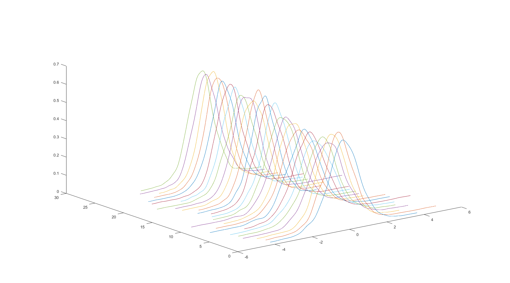
Figure 18: Factor SV model: Sequential one-step ahead predictive density estimates for the equally weighted portfolio of US industry stock return from 25/10/2005 to 29/11/2005 estimated using SMC-PG-batch-seq

Section 5.2 compares PHS and the approximate MCMC sampler of Kastner et al., (2017) for estimating the factor SV model. Figures 23 to 26 give results for the parameters $\tau^{2}_{\epsilon,s}$, $\mu_{\epsilon,s}$, and $\phi_{\epsilon,s}$, for $s=1,...,S$, and the factor loading matrix $\beta$ of the factor SV model. The figures show that although some parameters estimated using the approximate MCMC sampler are close to PHS, other parameters are quite different. The approximate MCMC sampler can be unreliable when estimating the parameters of the factor SV model.

Section 5.2 also investigates the performance of SMC-PG and SMC-PHS and compares them to PHS for estimating the factor SV model. Figures 19 to 22 show the estimates of $\tau^{2}_{\epsilon,s}$, $\mu_{\epsilon,s}$, and $\phi_{\epsilon,s}$, for $s=1,...,S$, and the factor loading matrix $\beta$ of the factor SV model. In general, the SMC-PG and SMC-PHS estimates are very close to the PHS estimates for all parameters, suggesting that SMC-PG is as accurate as SMC-PHS and faster for estimating the standard factor SV model.

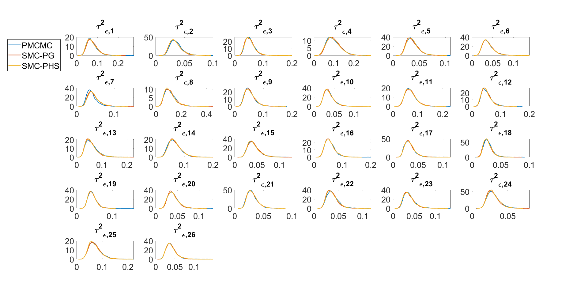
Figure 19: Factor SV model: The marginal posterior density plots of the parameters $\tau^{2}_{\epsilon,s}$ for $s=1,...,S$ estimated using PMCMC (PHS), SMC-PG, and SMC-PHS methods.

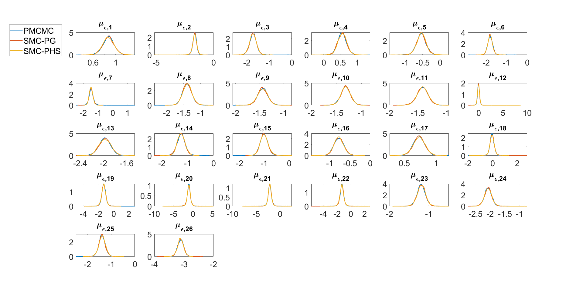
Figure 20: The marginal posterior density plots of the parameters $\mu_{\epsilon,s}$ for $s=1,...,S$ estimated using PMCMC (PHS), SMC-PG, and SMC-PHS methods.

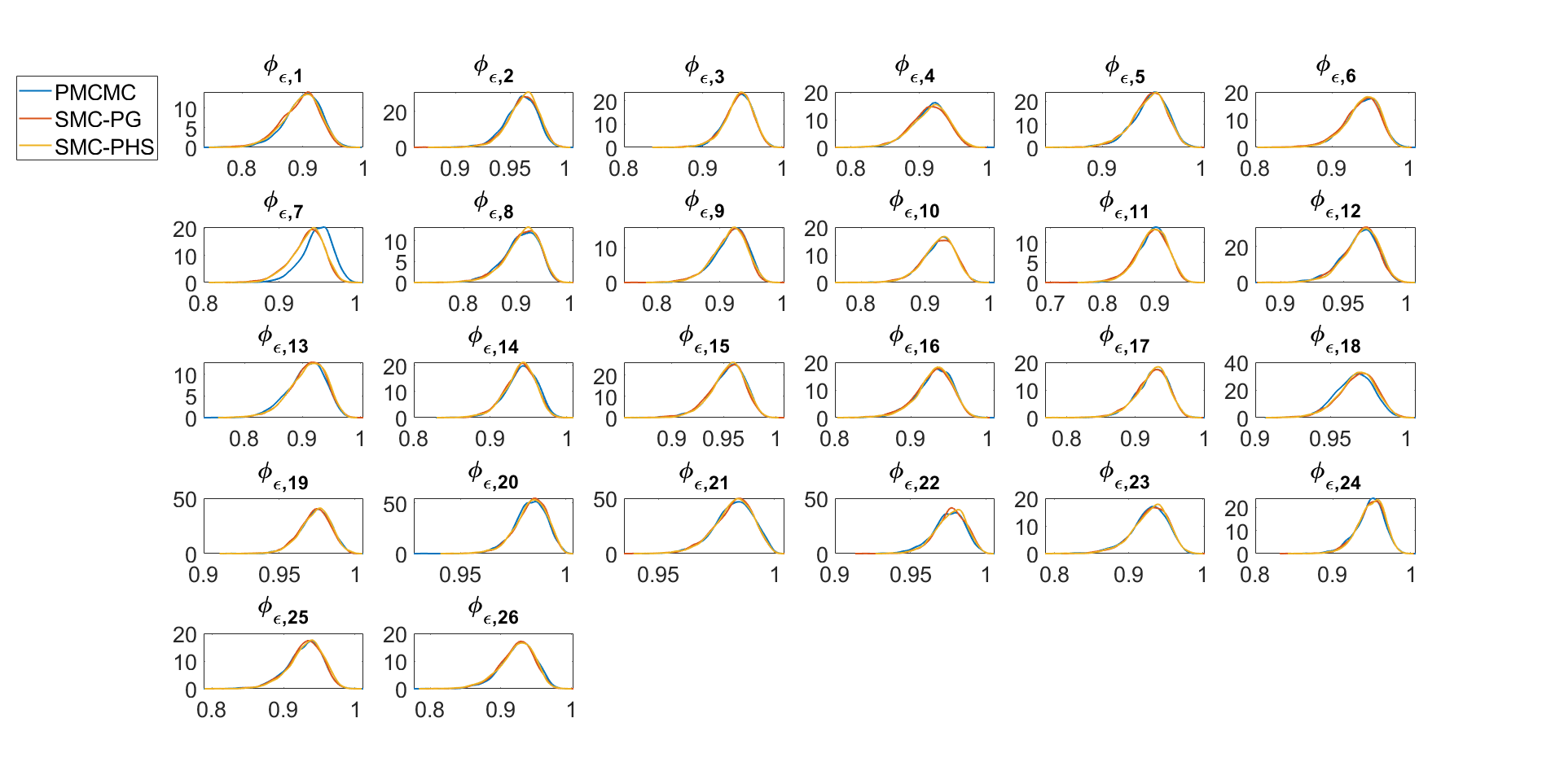
Figure 21: The marginal posterior density plots of the parameters $\phi_{\epsilon,s}$ for $s=1,...,S$ estimated using PMCMC (PHS), SMC-PG, and SMC-PHS methods.

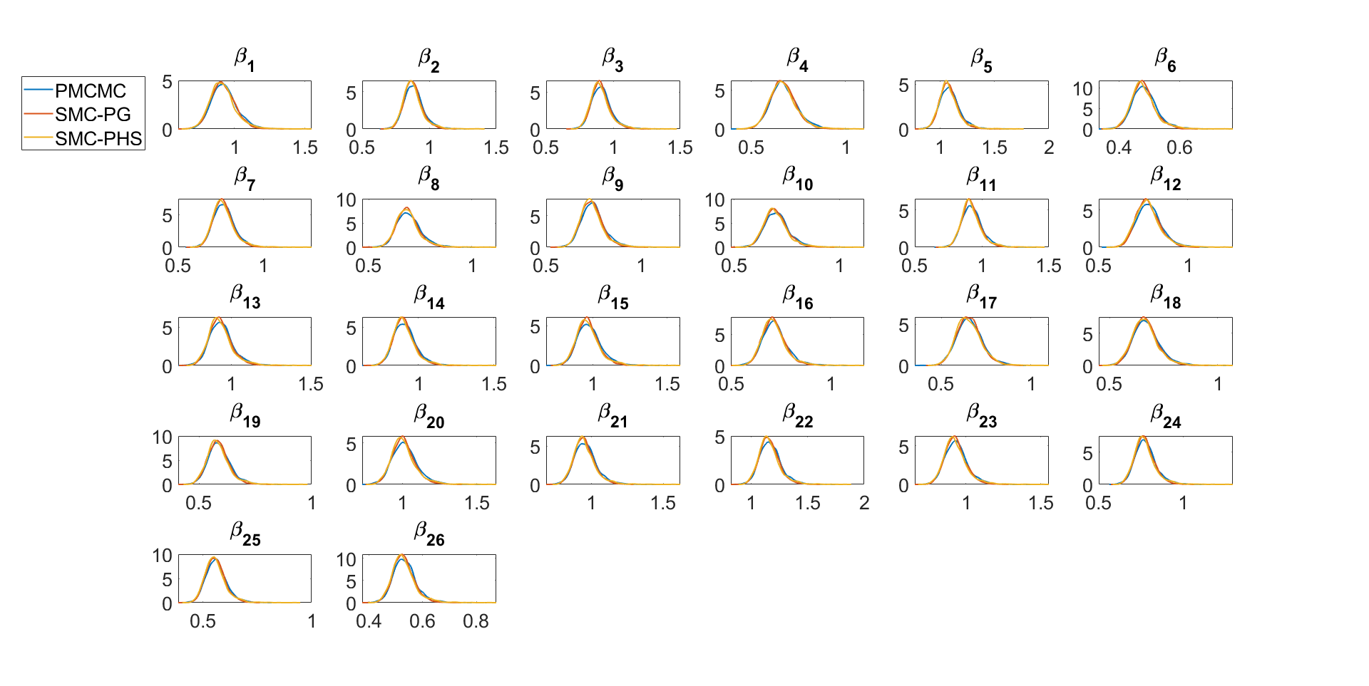
Figure 22: The marginal posterior density plots of the parameters $\beta$ estimated using PMCMC (PHS), SMC-PG and SMC-PHS methods.

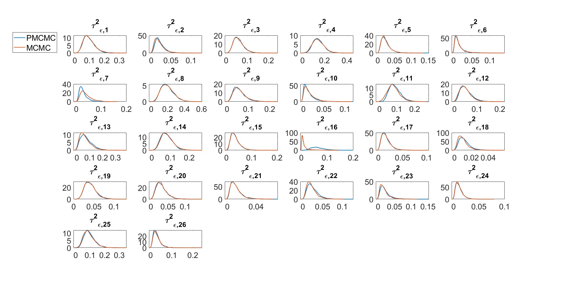
Figure 23: The marginal posterior density plots of the parameters $\tau^{2}_{\epsilon,s}$ for $s=1,...,S$ estimated using PMCMC (PHS) and MCMC of Kastner et al., (2017) methods.

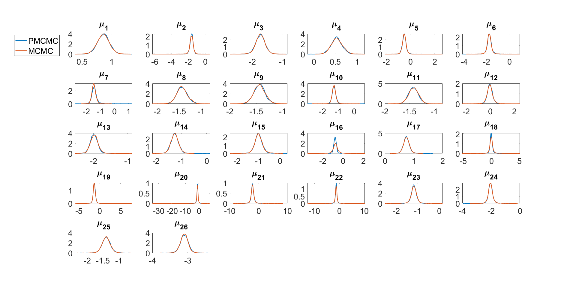
Figure 24: The marginal posterior density plots of the parameters $\mu_{\epsilon,s}$ for $s=1,...,S$ estimated using PMCMC (PHS) and MCMC of Kastner et al., (2017) methods.

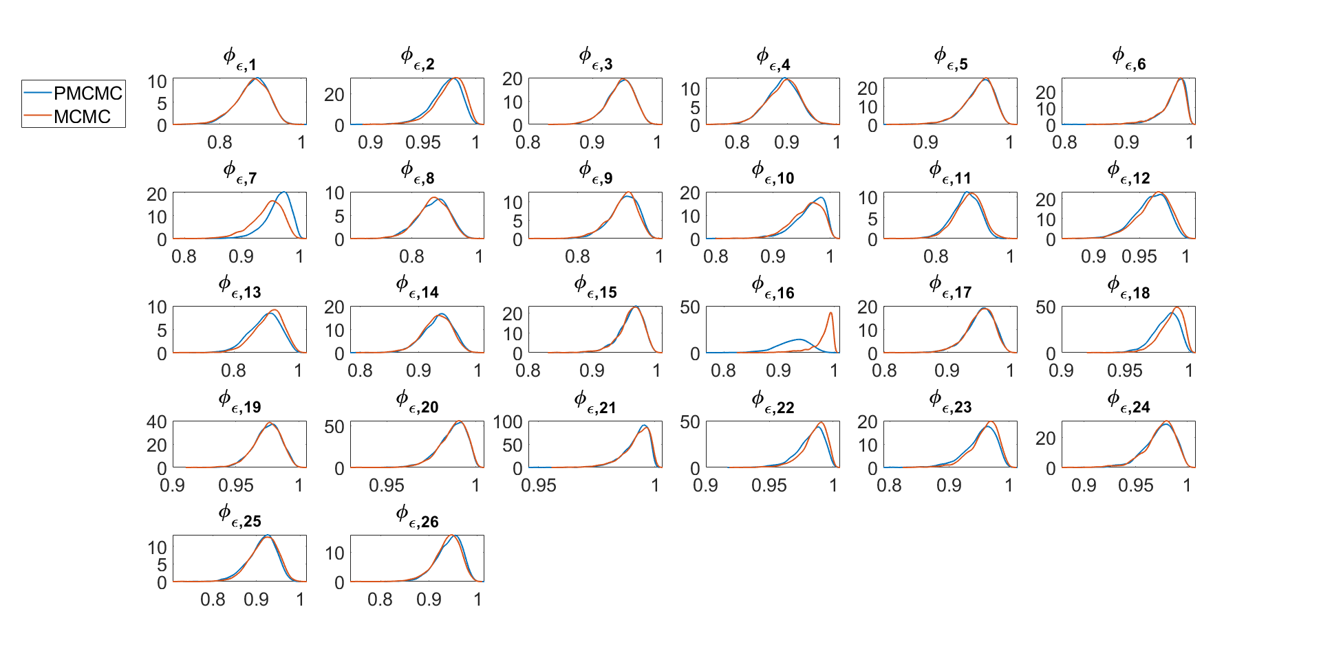
Figure 25: The marginal posterior density plots of the parameters $\phi_{\epsilon,s}$ for $s=1,...,S$ estimated using PMCMC (PHS) and MCMC of Kastner et al., (2017) methods.

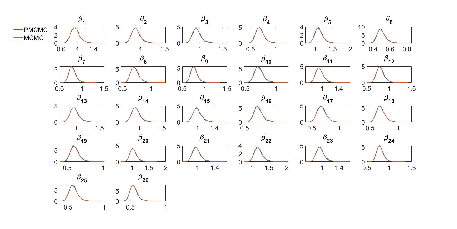
Figure 26: The marginal posterior density plots of the parameters $\beta$ estimated using PMCMC (PHS) and MCMC of Kastner et al., (2017) methods.

References

- Aguilar and West, (2000) Aguilar, O. and West, M. (2000). Bayesian dynamic factor models and portfolio allocation. Journal of Business and Economics Statistics, 18(3):338–357.
- Andrieu et al., (2010) Andrieu, C., Doucet, A., and Holenstein, R. (2010). Particle Markov chain Monte Carlo methods. Journal of the Royal Statistical Society, Series B, 72:1–33.
- Beskos et al., (2016) Beskos, A., Jasra, A., Kantas, N., and Thiery, A. H. (2016). On the convergence of adaptive sequential Monte Carlo methods. The Annals of Applied Probability, 26(2):1111–1146.
- Betancourt, (2017) Betancourt, M. (2017). A conceptual introduction to Hamiltonian Monte Carlo. arXiv preprint arXiv:1701.02434.
- Bodnar et al., (2017) Bodnar, T., Mazur, S., and Okhrin, Y. (2017). Bayesian estimation of the global minimum variance portfolio. European Journal of Operation Research, 256:292–307.
- Brix et al., (2018) Brix, A. F., Lunde, A., and Wei, W. (2018). A general Schwartz model for energy spot price - estimation using a particle MCMC method. Energy economics, 72:560–582.
- Buchholz et al., (2020) Buchholz, A., Chopin, N., and Jacob, P. E. (2020). Adaptive tuning of Hamiltonian Monte Carlo within sequential Monte Carlo. Bayesian Analysis, pages 1–27.
- Chan et al., (2017) Chan, J., Gonzalez, R. L., and Strachan, R. W. (2017). Invariant inference and efficient computation in the static factor model. Journal of American Statistical Association.
- Chib, (1998) Chib, S. (1998). Estimation and comparison of multiple change-point models. Journal of Econometrics, 86(2):221–241.
- Chib and Jeliazkov, (2001) Chib, S. and Jeliazkov, I. (2001). Marginal likelihood from the Metropolis-Hastings output. Journal of American Statistical Association, 96(453):270–281.
- Chib et al., (2006) Chib, S., Nardari, F., and Shephard, N. (2006). Analysis of high dimensional multivariate stochastic volatility models. Journal of Econometrics, 134:341–371.
- Chopin, (2004) Chopin, N. (2004). Central limit theorem for sequential Monte carlo methods and its application to Bayesian inference. The Annals of Statistics, 32:2385–2411.
- Chopin et al., (2013) Chopin, N., Jacob, P. E., and Papaspiliopoulos, O. (2013). SMC2: an efficient algorithm for sequential analysis of state space models. Journal of Royal Statistical Society Series B, 75(3):397–426.
- Chopin and Singh, (2015) Chopin, N. and Singh, S. S. (2015). On particle Gibbs sampling. Bernoulli, 21(3):1855–1883.
- Choppala et al., (2016) Choppala, P., Gunawan, D., Chen, J., Tran, M. N., and Kohn, R. (2016). Bayesian inference for state space models using block and correlated pseudo marginal methods. arXiv:1612.07072v1.
- Del Moral, (2004) Del Moral, P. (2004). Feynman-Kac Formulae: Genealogical and Interacting Particle Systems with Applications. Springer, New York.
- Del Moral et al., (2006) Del Moral, P., Doucet, A., and Jasra, A. (2006). Sequential Monte Carlo samplers. Journal of the Royal Statistical Society, Series B, 68:411–436.
- Del Moral et al., (2012) Del Moral, P., Doucet, A., and Jasra, A. (2012). An adaptive Sequential Monte Carlo for approximate Bayesian computation. Statistics and Computing, pages 1009–1020.
- Deligiannidis et al., (2018) Deligiannidis, G., Doucet, A., and M.Pitt (2018). the correlated pseudomarginal method. Journal of Royal Statistical Society Series B, 80(5):839–870.
- Duan and Fulop, (2015) Duan, J. C. and Fulop, A. (2015). Density-tempered marginalised sequential Monte Carlo samplers. Journal of Business and Economics Statistics, 33(2):192–202.
- Duane et al., (1987) Duane, S., Kennedy, A. D., Pendleton, B. J., and Roweth, D. (1987). Hybrid Monte Carlo. Physics Letters B, 195(2):216–222.
- Dufays, (2016) Dufays, A. (2016). Evolutionary sequential monte carlo samplers for change-point models. Econometrics, 4(1):12.
- Fulop and Li, (2013) Fulop, A. and Li, J. (2013). Efficient learning via simulation: A marginalised resample-move approach. Journal of Econometrics, 176:146–161.
- Garthwaite et al., (2015) Garthwaite, P. H., Fan, Y., and Sisson, S. A. (2015). Adaptive optimal scaling of Metropolis-Hastings algorithms using the Robbins-Monro process. Communications in Statistics - Theory and Methods, 45(17):5098–5111.
- Gerlach et al., (1998) Gerlach, R., Carter, C., and Kohn, R. (1998). Diagnostics for time series analysis. Journal of Time Series Analysis, 20(3).
- Geweke and Zhou, (1996) Geweke, J. F. and Zhou, G. (1996). Measuring the pricing error of the arbitrage pricing theory. Review of Financial Studies, 9:557–587.
- Girolami and Calderhead, (2011) Girolami, M. and Calderhead, B. (2011). Riemannian manifold Langevin and Hamiltonian Monte Carlo methods. Journal of Royal Statistician Society Series B, 73(2):123–214.
- (28) Gunawan, D., Carter, C., and Kohn, R. (2020a). On scalable particle Markov chain Monte Carlo. arXiv:1804.04359v3.
- (29) Gunawan, D., Dang, K. D., Quiroz, M., Kohn, R., and Tran, M. N. (2020b). Subsampling sequential Monte Carlo for static Bayesian models. Statistics and Computing, 30:1741–1758.
- Hoffman et al., (2013) Hoffman, M. D., Blei, D. M., Wang, C., and Paisley, J. (2013). Stochastic variational inference. Journal of Machine Learning Research, 14:1303–1347.
- Hoffman and Gelman, (2014) Hoffman, M. D. and Gelman, A. (2014). The No-U-Turn sampler: adaptively setting path length in Hamiltonian Monte Carlo. Journal of Machine Learning Research, 15:1593–1623.
- Holton, (2003) Holton, G. A. (2003). Value-at-risk: theory and practice. Academic Press.
- Hosszejni and Kastner, (2019) Hosszejni, D. and Kastner, G. (2019). Modeling univariate and multivariate stochastic volatility in R with stochvol and factorstochvol. arXiv:1906.12123.
- Ignatieva et al., (2015) Ignatieva, K., Rodrigues, P., and Seeger, N. (2015). Empirical analysis of affine versus nonaffine variance specifications in jump-diffusion models for equity indices. Journal of Business and Economic Statistics, 33(1):68–75.
- Jensen and Maheu, (2010) Jensen, M. J. and Maheu, J. M. (2010). Bayesian semiparametric stochastic volatility modeling. Journal of Econometrics, 157(2):306–316.
- Johansen, (2015) Johansen, A. M. (2015). On block, tempering, particle MCMC for systems identification. Proceedings of 17th IFAC Symposium on System Identification.
- Kass and Raftery, (1995) Kass, R. E. and Raftery, A. E. (1995). Bayes factors. Journal of American Statistical Association, 90(430):773–795.
- Kastner, (2019) Kastner, G. (2019). Sparse Bayesian time-varying covariance estimation in many dimensions. Journal of Econometrics, 210(1):98–115.
- Kastner et al., (2017) Kastner, G., Schnatter, S. F., and Lopes, H. F. (2017). Efficient bayesian inference for multivariate factor stochastic volatility models. Journal of Computational and Graphical Statistics, 26(4):905–917.
- Kim et al., (1998) Kim, S., Shephard, N., and Chib, S. (1998). Stochastic volatility: likelihood inference and comparison with ARCH models. The Review of Economic Studies, 65(3):361–393.
- Lindsten et al., (2014) Lindsten, F., Jordan, M. I., and Schon, T. B. (2014). Particle Gibbs with ancestor sampling. Journal of Machine Learning Research, 15:2145–2184.
- Lindsten and Schon, (2013) Lindsten, F. and Schon, T. B. (2013). Backward simulation methods for Monte Carlo statistical inference. Foundation and Trends in machine learning, 6(1):1–43.
- Mendes et al., (2020) Mendes, E. F., Gunawan, D., Carter, C. K., and Kohn, R. (2020). A flexible particle Markov chain Monte Carlo method. Statistics and Computing, 30:783–798.
- Nardari and Scruggs, (2007) Nardari, F. and Scruggs, J. T. (2007). Bayesian analysis of linear factor models with latent factors, multivariate stochastic volatility, and apt pricing restrictions. Journal of Financial and Quantitative Analysis, 42(4):857–891.
- Neal, (2001) Neal, R. (2001). Annealed importance sampling. Statistics and Computing, 11:125–139.
- Neal, (2011) Neal, R. M. (2011). MCMC using Hamiltonian dynamics. Handbook of Markov chain Monte Carlo, Chapman and Hall/CRC.
- Nemeth et al., (2016) Nemeth, C., Sherlock, C., and Fearnhead, P. (2016). Particle Metropolis-adjusted Langevin algorithms. Biometrika, 103(3):701–717.
- Olsson and Ryden, (2011) Olsson, J. and Ryden, T. (2011). Rao-Blackwellisation of particle Markov chain Monte Carlo methods using forward filtering backward sampling. IEEE Transactions on Signal Processing, 59(10):4606–4619.
- Pitt et al., (2012) Pitt, M. K., Silva, R. S., Giordani, P., and Kohn, R. (2012). On some properties of Markov chain Monte Carlo simulation methods based on the particle filter. Journal of Econometrics, 171(2):134–151.
- Shephard, (1994) Shephard, N. E. (1994). Partial non-Gaussian state space models. Biometrika, 81:115–131.
- Sherlock et al., (2015) Sherlock, C., Thiery, A., Roberts, G., and Rosenthal, J. (2015). On the efficiency of pseudo-marginal random walk Metropolis algorithms. Annals of Statistics, 43(1):238–275.
- Smith, (1985) Smith, J. Q. (1985). Diagnostic checks of non-standard time series models. Journal of Forecasting, 4:283–291.
- South et al., (2019) South, L. F., Pettitt, A. N., and Drovandi, C. C. (2019). Sequential Monte Carlo samplers with independent Markov chain Monte Carlo proposals. Bayesian Analysis, 14(3):753–776.
- Stein and Stein, (1991) Stein, E. and Stein, J. (1991). Stock price distributions with stochastic volatility: an analytic approach. Review of Financial Studies, 4:727–752.
- Stephens, (1974) Stephens, M. A. (1974). EDF statistics for goodness of fit and some comparisons. Journal of American Statistical Association, 69:730–737.
- Stramer and Bognar, (2011) Stramer, O. and Bognar, M. (2011). Bayesian inference for irreducible diffusion processes using the pseudo-marginal approach. Bayesian Analysis, 6(2):231–258.
- Whiteley, (2010) Whiteley, N. (2010). Discussion on particle Markov chain Monte Carlo methods. Journal of the Royal Statistical Society Series B, 72(3):306–307.
- Zhou et al., (2014) Zhou, X., Nakajima, J., and West, M. (2014). Bayesian forecasting and portfolio decisions using dynamic dependent sparse factor models. International Journal of Forecasting, 30(4):963–980.