Duality and free energy analyticity bounds for few-body Ising models
with extensive homology rank

Abstract

We consider pairs of few-body Ising models where each spin enters a bounded number of interaction terms (bonds), such that each model can be obtained from the dual of the other after freezing $k$ spins on large-degree sites. Such a pair of Ising models can be interpreted as a two-chain complex with $k$ being the rank of the first homology group. Our focus is on the case where $k$ is extensive, that is, scales linearly with the number of bonds $n$. Flipping any of these additional spins introduces a homologically non-trivial defect (generalized domain wall). In the presence of bond disorder, we prove the existence of a low-temperature weak-disorder region where additional summation over the defects have no effect on the free energy density $f(T)$ in the thermodynamical limit, and of a high-temperature region where in the ferromagnetic case an extensive homological defect does not affect $f(T)$. We also discuss the convergence of the high- and low-temperature series for the free energy density, prove the analyticity of limiting $f(T)$ at high and low temperatures, and construct inequalities for the critical point(s) where analyticity is lost. As an application, we prove multiplicity of the conventionally defined critical points for Ising models on all $\{f,d\}$ tilings of the infinite hyperbolic plane, where $df/(d+f)>2$. Namely, for these infinite graphs, we show that critical temperatures with free and wired boundary conditions differ, $T_{c}^{(\mathrm{f})}<T_{c}^{(\mathrm{w})}$.

I Introduction

Singular behavior associated with a phase transition may emerge only in the thermodynamical limit, as the system size goes to infinity. One example are spin models on any finite-dimensional lattice, where both the interaction strength and its range are finite. Then the thermodynamical limit is well defined thanks to the fact that boundary contribution scales sublinearly with the system sizeGriffiths (1972). Respectively, e.g., in the case of an Ising model, the same transition can be alternatively defined as the temperature where spontaneous magnetization appears, spin susceptibility diverges, spin correlations start to decay exponentially, domain wall tension is lost, or as a singular point of the free energyLebowitz (1977); Gruber and Lebowitz (1978); Lebowitz and Pfister (1981); Griffiths (1972).

Situation is different if we are interested in non-local models, where the size of the boundary scales linearly with the size of the subset induced by any finite set of vertices. Examples include models on infinite transitive expander graphs like a degree-regular treeLyons (1989, 2000) or regular $\{f,d\}$ tilings of the hyperbolic plane, with $(f-2)(d-2)>2$. Here, the bulk quantities cannot be uniquely defined, and the transition temperature may depend on both the quantity being probed and the boundary conditions used to define the infinite-graph limit.

Infinite hyperbolic tilings provide a natural short-scale regularization for a space with constant negative curvature. Interest in quantum field theory models on curved space-time is motivated by quantum gravity and, in particular, the AdS/CFT correspondenceBirrel and Davies (1982); Cognola et al. (1993); Camporesi (1991); Miele and Vitale (1997); Doyon (2003); Evenbly and Vidal (2011); Matsueda et al. (2013). There is an independent interest in models on curved spaces in statistical mechanics and condensed matter communities, e.g., since curvature can serve as an additional parameter to drive the criticality, or as a way to introduce geometrical frustration in toy models of amorphous solids, supercooled liquids, and metallic glassesNelson (1983); Tarjus et al. (2005); Vitelli et al. (2006); Sausset and Tarjus (2007); Giomi and Bowick (2007); Turner et al. (2010); Garcia et al. (2015); Benedetti (2015). Models like percolation on more general expander graphs and various random graph ensembles are also common in network theory, e.g., such models occurred in relation to internet stability and spread of infectious diseasesCohen et al. (2000); Albert and Barabási (2002); Gai and Kapadia (2010); Börner et al. (2007); Sander et al. (2002); da Fontoura Costa et al. (2011); Danon et al. (2011). Finally, the strongest motivation to study non-local Ising models comes from their relationDennis et al. (2002); Kovalev and Pryadko (2015); Kovalev et al. (2018) to certain families of finite-rate quantum error-correcting codes (QECCs).

In a companion paperKovalev et al. (2018) devoted to error-correcting properties of QECCs, three of us studied pairs of weakly-dual few-body Ising models where each spin enters a bounded number of interaction terms (bonds). Each model can be obtained from the exact dual of the other after freezing $k$ spins which enter a large number of bonds. For the related QECC, $k$ is the number of encoded qubits, and its ratio to the number of bonds, $R\equiv k/n$, is the code rate. One can also map such a pair of Ising models to a $2$-chain complex $\Sigma$, in which case $k$ is the rank of the first homology group $H_{1}(\Sigma)$. In particular, in Ref. Kovalev et al., 2018 we introduced the homological difference $\Delta F\geq 0$, the difference of the free energies of two models with and without the additional summation over the homological defects, and gave the sufficient conditions for the existence of a low-temperature low-disorder region on the phase diagram where in the large-system limit $\Delta F=0$.

In the present work we study duality and phase transitions in general Ising models with the help of the specific homological difference scaled by the number of bonds, $\Delta f=\Delta F/n$, focusing on the case where the homology rank $k$ scales linearly with the number of bonds $n$. Upon duality $\Delta f$ is mapped to $R\ln 2-\Delta f^{*}$, where $\Delta f^{*}$ is the homological difference for the other model in the pair, at the dual temperature. Existence of a low-temperature homological region where asymptotically $\Delta f=0$ implies that at high temperatures $\Delta f^{*}=R\ln 2$; with $R>0$ this implies the existence of at least two distinct points where $\Delta f$ is non-analytic as a function of temperature. Combining with the analysis of convergence of the high-temperature series expansion for the free energy density, we obtain several bounds for critical temperatures associated with the non-analyticity of $\Delta f$ and limiting free energy densities of the two models. Main result is the inequality for the change of phase transition temperature due to summation over the homological defects. As an application, we prove multiplicity of the conventionally defined critical points for Ising models on all $\{f,d\}$ tilings of the hyperbolic plane with $df/(d+f)>2$. That is, we show that transition temperatures with wired and free boundary conditions differ, $T_{c}^{(\mathrm{w})}>T_{c}^{(\mathrm{f})}$, which extends the results of Refs. Wu, 2000; Schonmann, 2001; Häggström et al., 2002.

The paper is organized as follows. We introduce the notations and review some known facts from theory of general Ising models and theory of QECCs in Sec. II. Our results are given in Sec. III, where we first discuss properties of the homological difference $\Delta f$, analyze the convergence and analyticity of free energy density for a sequence of weakly-dual Ising model pairs, and finally apply the obtained results to Ising models on $\{f,d\}$ tilings of the hyperbolic plane, additionally illustrating the conclusions with numerical simulations. We summarize the results and list some related open questions in Sec. IV. Most of the proofs are given in the Appendices.

II Notations and background

We consider general Ising models in Wegner’s formWegner (1971), which describes joint probability distribution of $r\equiv|{\cal V}|$ Ising spin variables, $S_{v}\in\{-1,1\}$, associated with elements of the vertex set, ${\cal V}$,

$$\mathop{\rm Prob}\nolimits_{\mathbf{e}}[\{S\};\Theta;K,h]={1\over Z}\prod_{b\in\mathcal{B}}e^{K(-1)^{e_{b}}R_{b}}\prod_{v\in\mathcal{V}}e^{hS_{v}},$$ (1)

where each bond $R_{b}\equiv\prod_{v\in{\cal V}}S_{v}^{\Theta_{vb}}$, $b\in{\cal B}$, $|{\cal B}|=n$, is a product of the spin variables corresponding to non-zero positions in the corresponding column of the $r\times n$ binary coupling matrix $\Theta$, the binary “error” vector $\mathbf{e}$ with components $e_{b}$, $b\in{\cal B}$, describes quenched disorder, and the dimensionless coupling coefficients are $K\equiv\beta J$ and $h\equiv\beta h^{\prime}$, where $J$ is the Ising exchange constant, $h^{\prime}$ is the magnetic field, and $\beta\equiv 1/T$ the inverse temperature in energy units. The normalization constant in Eq. (1) is the partition function,

$$Z\equiv Z_{\mathbf{e}}(\Theta;K,h)\equiv\sum_{\{S_{v}=\pm 1\}}\prod_{b\in{\cal B}}e^{K(-1)^{e_{b}}R_{b}}\prod_{v\in\mathcal{V}}e^{hS_{v}}.$$ (2)

The partition function is commonly written in terms of the corresponding logarithm, the free energy, $F=-\ln Z$, or the free energy density (per bond), $f=F/n$.

The binary coupling matrix $\Theta$ in Eq. (1) can be interpreted geometrically in terms of a bipartite Tanner graphTanner (1981), or, equivalently, as the vertex-edge incidence matrix for a hypergraph $\mathcal{H}=(\mathcal{V},\mathcal{B})$ with vertex set $\mathcal{V}$ and hyperedge (bond) set $\mathcal{B}$, with each hyperedge $b\in\mathcal{B}$ a non-empty subset of the vertex set, $b\subseteq\mathcal{V}$. In comparison, in a (simple undirected) graph $\mathcal{G}=(\mathcal{V},\mathcal{E})$, each edge $b\in\mathcal{E}$ is an unordered pair of vertices, $b=\{i,j\}\subseteq\mathcal{V}$. The degree $d_{v}$ of a vertex $v\in\mathcal{V}$ in a (hyper)graph is the number of edges that contain $v$, it is equal to the number of non-zero entries in the $v$ th row of the vertex-edge incidence matrix $\Theta$. Similarly, the size of an edge in a hypergraph is called its degree, $d_{b}=|b|$, $b\in\mathcal{B}$. In a graph, all edges are pairs of vertices, and all columns of the incidence matrix $\Theta$ have exactly two non-zero entries.

The probability distribution (1) can be characterized via the corresponding marginals, the spin correlations

$$\langle S_{\cal A}\rangle\equiv\sum_{\{S_{v}=\pm 1\}}S_{\cal A}\mathop{\rm Prob}\nolimits_{\mathbf{e}}(\{S\};\Theta;K,h),$$ (3)

where ${\cal A}\subseteq{\cal V}$ is a set of vertices, $S_{\mathcal{A}}=\prod_{v\in\mathcal{A}}S_{v}$; by convention, $S_{\emptyset}=1$. At $h=0$, on a finite system and with $\mathbf{e}=\mathbf{0}$, non-zero expectation is obtained for the sets (and only the sets) that can be constructed as products of bondsWegner (1971),

$$S_{\cal A}=\prod_{b:m_{b}\neq 0}R_{b}=\prod_{v}\prod_{b}S_{v}^{\Theta_{vb}m_{b}},$$ (4)

where bonds in the product correspond to non-zero positions $m_{b}\neq 0$ in the binary vector $\mathbf{m}\in\mathbb{F}_{2}^{n}$ of magnetic charges. A number of correlation inequalities for spin averages have been constructed, see, e.g., Refs. Percus, 1975; Shlosman, 1981. Particularly important for this work are Griffiths-Kelly-Sherman (GKS) inequalitiesGriffiths (1967); Kelly and Sherman (1968),

$$\langle S_{\cal A}\rangle \geq 0,$$ (5)

$$\langle S_{\cal A}S_{\cal B}\rangle \geq \langle S_{\cal A}\rangle\langle S_{\cal B}\rangle,$$ (6)

valid in the ferromagnetic case, $\mathbf{e}=\mathbf{0}$, for any ${\cal A},{\cal B}\subseteq{\cal V}$.

The second GKS inequality (6) can also be writtenGriffiths (1967); Kelly and Sherman (1968) in terms of the derivative of $\langle S_{\cal A}\rangle$ with respect to $K_{\mathcal{B}}$, the dimensional coupling constant corresponding to the product of spins $S_{\mathcal{B}}$,

$${d\langle S_{\mathcal{A}}\rangle\over dK_{\mathcal{B}}}\geq 0.$$ (7)

This implies the monotonicity of any average with respect to all coupling constants and, as a consequence, the existence of two extremal Gibbs states describing (generally different) thermodynamical limit(s) for the Ising model on an infinite hypergraph $\mathcal{H}=(\mathcal{V},\mathcal{B})$, with free and wired boundary conditions, respectively. Namely, one considers an increasing sequence $\mathcal{V}_{t}$, $t\in\mathbb{N}$, of sets of vertices, $\mathcal{V}_{t}\subsetneq\mathcal{V}_{t+1}\subset\mathcal{\mathcal{V}}$ which converges weakly to $\mathcal{V}=\cup_{t\in\mathbb{N}}\mathcal{V}_{t}$, and the sequence of sub-hypergraphs $\mathcal{H}_{t}=(\mathcal{V}_{t},\mathcal{B}_{t})$ induced by the sets $\mathcal{V}_{t}$. For each $\mathcal{H}_{t}$, consider also the hypergraph $\mathcal{H}_{t}^{\prime}=(\mathcal{V}_{t}^{\prime},\mathcal{B}_{t}^{\prime})$, obtained from $\mathcal{H}$ by contracting all vertices outside $\mathcal{V}_{t}$ into one. Denote the vertex-edge incidence matrices of $\mathcal{H}_{t}$ and $\mathcal{H}_{t}^{\prime}$ as $\Theta_{t}^{\mathrm{f}}$ and $\Theta_{t}^{\mathrm{w}}$, respectively. Here “f” and “w” stand for “free” and “wired” boundary conditions in the Ising models (1) defined with the help of these matrices. Clearly, $\mathcal{H}_{t}$ can be obtained from $\mathcal{H}_{t+1}$ by reducing some couplings to zero, while $\mathcal{H}_{t}^{\prime}$ can be obtained from $\mathcal{H}_{t+1}^{\prime}$ by increasing some couplings to infinity. This implies that for any set of vertices $\mathcal{A}\subset\mathcal{V}$, and $t$ large enough so that $\mathcal{A}\subset\mathcal{V}_{t}$, the averages $\langle S_{\mathcal{A}}\rangle_{t}^{\mathrm{f}}\leq\langle S_{\mathcal{A}}\rangle_{t}^{\mathrm{w}}$ are, respectively, non-decreasing and non-increasing with $t$. They are also bounded, which proves the existence of the corresponding pointwise limits, $\langle S_{\mathcal{A}}\rangle^{\mathrm{f}}\leq\langle S_{\mathcal{A}}\rangle^{\mathrm{w}}$ at any $K$ and $h$.

The two limits are known to coincide Griffiths (1972) for degree-limited graphs embeddable in $D$-dimensional space, e.g., the hypercubic lattice $\mathbb{Z}^{D}$. Indeed, the increasing sequence of subgraphs $\mathcal{G}_{t}=(\mathcal{V}_{t},\mathcal{E}_{t})$ can be chosen so that the boundary grows sublinearly with the total number of spins $|\mathcal{V}_{t}|$. Such a property is violated in the case of a non-amenable graph $\mathcal{G}$, which has a non-zero edge expansion (Cheeger) constant, $\iota_{E}(\mathcal{G})>0$, defined as

$$\iota_{E}(\mathcal{G})\equiv\sup_{\mathcal{W}\subset\mathcal{V}:|\mathcal{W}|<\infty}\frac{|\partial_{E}\mathcal{W}|}{|\mathcal{W}|},$$ (8)

where $\partial_{E}(\mathcal{W})$ is the set of edges connecting $\mathcal{W}$ with its complement, $\mathcal{V}\setminus\mathcal{W}$. The dependence of the critical temperatures (as seen by the magnetization) on the boundary conditions, $T_{c}^{\mathrm{w}}>T_{c}^{\mathrm{f}}$, where the superscripts stand for “wired” and “free” boundary conditions, respectively, is called the “multiplicity” of critical pointsWu (2000); Schonmann (2001); Häggström et al. (2002). Examples are the infinite $d$-regular trees $\mathcal{T}_{d}$ (in this case $T_{c}^{\mathrm{f}}=0$, $T_{c}^{\mathrm{w}}=(d-1)^{-1}$, see, e.g., Ref. Lyons, 1989), and the regular $\{f,d\}$ tilings ${\bf H}(f,d)$ of the infinite hyperbolic plane, $df/(f+d)>2$, where in each vertex $d$ regular $f$-gons meet. In the latter case multiplicity of the critical points have been demonstrated for self-dual graphs, $d=f$, and for graphs with large enough curvature Wu (2000); Schonmann (2001); Häggström et al. (2002). In Sec. III.3 we prove the multiplicity of critical points for all hyperbolic tilings ${\bf H}(f,d)$ with $df/(d+f)>2$.

Another important result for the Ising model (1) is the duality transformationKramers and Wannier (1941); Wegner (1971). In particular, in the absence of bond disorder, $\mathbf{e}=0$, and at $h=0$, one has

$$Z_{\mathbf{0}}(\Theta;K)=Z_{\mathbf{0}}(\Theta^{*};K^{*})\,2^{r-n_{g}^{*}}\left(\sinh K\cosh K\right)^{n/2},$$ (9)

where $K^{*}$ is the Kramers-Wannier dual of $K$, namely $\tanh{K}^{*}=e^{-2{K}}$, the degeneracy $n_{g}^{*}=r^{*}-\mathop{\rm rank}\Theta^{*}$ ($2^{n_{g}^{*}}$ is the number of distinct ground-state spin configurations in the dual representation), and $\Theta^{*}$ is a binary $r^{*}\times n$ matrix exactly dual to $\Theta$ (binary rank is used),

$$\Theta^{*}\Theta^{T}=0,\quad\mathop{\rm rank}\Theta+\mathop{\rm rank}\Theta^{*}=n.$$ (10)

Notice that in Eq. (9), and elsewhere in this work, we simplify the notations by suppressing the argument corresponding to a zero magnetic field, $h=0$.

Exact duality also works in the presence of sign bond disorder, except the corresponding bonds (“electric charges”) are mapped by duality to extra factors in front of the exponent, “magnetic charges”. The resulting expression is not positive-definite and thus cannot be interpreted as a probability measure; instead it is proportional to the average of a product of the corresponding bonds. The duality in this case readsWegner (1971)

$${Z_{\mathbf{e}}(\Theta;K)\over Z_{\mathbf{0}}(\Theta;K)}=\left\langle\prod_{b\in\mathcal{B}}R_{b}^{e_{b}}\right\rangle_{\Theta^{*};K^{*}},$$ (11)

where the average on the right is computed in the dual model with all bonds ferromagnetic, cf. Eq. (4).

There is a natural notion of equivalence between defects $\mathbf{e}$ that produce identical averages in Eq. (11). For the electric charges in the l.h.s., equivalent are any two defects which differ by a linear combination of rows of $\Theta$, $\mathbf{e}\simeq\mathbf{e}^{\prime}=\mathbf{e}+\boldsymbol{\alpha}\Theta$, where $\boldsymbol{\alpha}$ is a length-$r$ binary vector. Such defects are related by Nishimori’s spin-glass gauge symmetryNishimori (2001) generated by local spin flips $\alpha_{v}\in\mathbb{F}_{2}$, $v\in\mathcal{V}$, and simultaneous update of the components of $\mathbf{e}$ on the adjacent bonds,

$$S_{v}\to(-1)^{\alpha_{v}}S_{v},\quad e_{b}\to e_{b}^{\prime}\equiv e_{b}+\sum\nolimits_{v}\alpha_{v}\Theta_{vb}.$$ (12)

For such a defect $\mathbf{e}$, it is convenient to introduce an invariant distance $d_{\mathbf{e}}$, the minimum number of flipped bonds among all defects in the same equivalence class,

$$d_{\mathbf{e}}\equiv d_{\mathbf{e}}(\Theta)=\min_{\boldsymbol{\alpha}}\mathop{\rm wgt}(\mathbf{e}+{\boldsymbol{\alpha}}\Theta),$$ (13)

where $\mathop{\rm wgt}(\mathbf{e})$ is the Hamming weight. An identical equivalence relation for the magnetic charges which define the product of spins in the r.h.s. of Eq. (11) can be interpreted as a result of introducing a product of (dual) bonds that form a cycle, i.e., does not change the spins that actually enter the average.

For a finite system and a finite $K>0$, both sides of Eq. (11) are strictly positive. The logarithm of the l.h.s. is proportional to the free energy increment due to the addition of the defect,

$$\delta_{\mathbf{e}}\equiv\delta_{\mathbf{e}}(\Theta;K)\equiv\ln Z_{\mathbf{0}}(\Theta;K)-\ln Z_{\mathbf{e}}(\Theta;K);$$ (14)

in turn, it is proportional to dimensionless defect tension

$$\tau_{\mathbf{e}}\equiv\tau_{\mathbf{e}}(\Theta;K)\equiv\delta_{\mathbf{e}}(\Theta;K)/d_{\mathbf{e}}.$$ (15)

Respectively, the scaling of the spin average in the r.h.s. of Eq. (11) with the minimum number of bonds in the product is called the area-law exponent,

$$\alpha_{\mathbf{e}}\equiv\alpha_{\mathbf{e}}(\Theta^{*};K^{*})=-d_{\mathbf{e}}^{-1}\ln\left\langle\prod_{b\in\mathcal{B}}R_{b}^{e_{b}}\right\rangle_{\Theta^{*};K^{*}}.$$ (16)

Second GKS inequality (6) implies subadditivity,

$$d_{\mathbf{e}_{1}+\mathbf{e}_{2}}\alpha_{\mathbf{e}_{1}+\mathbf{e}_{2}}\leq{d_{\mathbf{e}_{1}}\alpha_{\mathbf{e}_{1}}+d_{\mathbf{e}_{2}}\alpha_{\mathbf{e}_{2}}}.$$ (17)

Thus electric-magnetic duality (11) also implies an exact relation between the defect tension and area-law exponent in a pair of dual models,

$$\tau_{\mathbf{e}}(\Theta;K)=\alpha_{\mathbf{e}}(\Theta^{*};K^{*}).$$ (18)

Combined with Eq. (17), this implies subadditivity for defect free energy cost

$$\delta_{\mathbf{e}_{1}+\mathbf{e}_{2}}\leq\delta_{\mathbf{e}_{1}}+\delta_{\mathbf{e}_{2}}.$$ (19)

In the special case of a model with two-body couplings defined on a graph ${\cal G}=({\cal V},{\cal E})$, a single correlation decay exponent can be defined in terms of pair correlations,

$$\alpha\equiv\alpha(\mathcal{G};K)=\inf_{i,j\in\mathcal{V}}\left[-{\ln\langle S_{i}S_{j}\rangle\over d_{ij}}\right],$$ (20)

where $d_{ij}$ is the graph distance between $i$ and $j$. Subadditivity (17) implies that the value of $\alpha$ corresponds to that for pairs with large $d_{ij}$.

We are interested in the Ising models (1) with few-body couplings. More specifically, we consider weight-limited Ising models with vertex and bond degrees bounded by some fixed $\ell$ and $m$, respectively, so that $d_{v}\leq m$, $v\in{\cal V}$, and $d_{b}\leq\ell$, $b\in{\cal B}$. With fixed $\ell$ and $m$, we call such a model $(\ell,m)$-sparse. This refers to the sparsity of the corresponding coupling matrix $\Theta$: $\ell$ and $m$, respectively, are the maximum weights of a column and of a row of $\Theta$.

Further, we would like to consider models whose duals are in the same class of weight-limited Ising models, with some maximum vertex, $\ell^{*}$, and bond, $m^{*}$, degrees. However, such a condition would be very restrictive if one insists on the exact duality (10). For example, in the case of the square-lattice Ising model with periodic boundary conditions on an $L\times L$ square ($\ell=2$ and $m=4$), the dual model can be chosen to have the same vertex and bond degrees, $\ell^{*}=2$ and $m^{*}=4$, except for $k=2$ additional summations over periodic/antiperiodic boundary conditions in each direction. These summations can be introduced as additional spins entering $d_{v}\geq L$ bonds, where the lower bound is the length of the shortest domain wall on the $L\times L$ square-lattice tiling of a torus. The two additional summations give no contribution to the asymptotic free energy density at $L\to\infty$, both in the low- and high-temperature phases, and are often ignored.

Such a weak duality with additional defects for models on locally planar graphs can be generalized by considering a pair of weight-limited binary matrices with $n$ columns each, $G$ and $H$, such that their rows be mutually orthogonal, $G\,H^{T}=0$. Since we do not require exact duality (10), there are exactly

$$k\equiv n-\mathop{\rm rank}G-\mathop{\rm rank}H$$ (21)

distinct defect vectors $\mathbf{c}_{i}\in\mathbb{F}_{2}^{n}$, $i\in\{1,\ldots,k\}$, which are orthogonal to rows of $H$ and whose non-trivial linear combinations are linearly-independent from rows of $G$.

Just as for the spin glasses on locally planar graphs, the matrix $H$ can be used to define frustration, $\mathbf{s}\equiv\mathbf{e}\,H^{T}$, a gauge-invariant characteristic of bond disorder. As common in spin-glass theoryNishimori (2001), we will consider independent identically-distributed (i.i.d.) components of the quenched disorder vector $\mathbf{e}$, such that $e_{b}=1$ with probability $p$. The corresponding averages are denoted with square brackets, $[\,\boldsymbol{\cdot}\,]_{p}$.

In theory of quantum error correcting codesGottesman (1997); Calderbank et al. (1998); Nielsen and Chuang (2000); Preskill (2000), a pair of binary matrices with orthogonal rows, $G\,H^{T}=0$, can be used to define a Calderbank-Shor-SteaneCalderbank and Shor (1996); Steane (1996) (CSS) stabilizer code ${\cal Q}(G,H)$ which encodes $k$ qubits in $n$, see Eq. (21). Such a quantum code has a convenient representation in terms of classical binary codes. Given a matrix $G$ with $n$ columns, one defines the classical code $\mathcal{C}_{G}\subseteq\mathbb{F}_{2}^{n}$, a linear space of dimension $\mathop{\rm rank}G$ generated by the rows of $G$. One also defines the corresponding dual code $\mathcal{C}_{G}^{\perp}$ of all vectors in $\mathbb{F}_{2}^{n}$ orthogonal to rows of $G$; such a code is generated by the corresponding dual matrix (10), $\mathcal{C}_{G}^{\perp}\equiv\mathcal{C}_{G^{*}}$. By orthogonality, we necessarily have $\mathcal{C}_{H}\subseteq\mathcal{C}_{G}^{\perp}$ and $\mathcal{C}_{G}\subseteq\mathcal{C}_{H}^{\perp}$, where equality is achieved when the two matrices are exact dual of each other, in which case $k=0$. The defect vectors $\mathbf{c}$ are non-zero CSS codewords of $G$ type, $\mathbf{c}\in\mathcal{C}_{H}^{\perp}\setminus\mathcal{C}_{G}$; there are exactly $2^{k}-1$ inequivalent (mutually non-degenerateCalderbank et al. (1998)) vectors of this type. Similarly, there are also $2^{k}-1$ inequivalent $H$-type vectors $\mathbf{b}$ in $\mathcal{C}_{G}^{\perp}\setminus\mathcal{C}_{H}$, where equivalence is defined in terms of rows of $H$, $\mathbf{b}^{\prime}\simeq\mathbf{b}$ iff $\mathbf{b}^{\prime}=\mathbf{b}+\alpha^{T}H$. For any quantum code, important parameters are its rate, $R\equiv k/n$, and the distance, $d\equiv\min(d_{G},d_{H})$,

$$d_{G}\equiv\min_{\mathbf{c}\in\mathcal{C}_{H}^{\perp}\setminus\mathcal{C}_{G}}\mathop{\rm wgt}(\mathbf{c}),\quad d_{H}\equiv\min_{\mathbf{b}\in\mathcal{C}_{G}^{\perp}\setminus\mathcal{C}_{H}}\mathop{\rm wgt}(\mathbf{b}).$$ (22)

As yet another interpretation of the algebraic structure in the pair of weakly-dual Ising models with vertex-bond incidence matrices $G$ and $H$ of dimensions $r\times n$ and $r^{\prime}\times n$, respectively, consider a two-chain complex $\Sigma\equiv\Sigma(G,H)$,

$$\Sigma:\;C_{2}\equiv\mathbb{F}_{2}^{r^{\prime}}\stackrel{{\scriptstyle\partial_{2}}}{{\rightarrow}}C_{1}\equiv\mathbb{F}_{2}^{n}\stackrel{{\scriptstyle\partial_{1}}}{{\rightarrow}}C_{0}\equiv\mathbb{F}_{2}^{r},$$ (23)

where the modules $C_{j}$, $j\in\{0,1,2\}$ are the linear spaces of binary vectors with dimensions $r$, $n$, and $r^{\prime}$, respectively, and the boundary operators $\partial_{1}$ and $\partial_{2}$ are two linear maps defined by the matrices $G$ and $H^{T}$. The required composition property, $\partial_{1}\circ\partial_{2}=0$, is guaranteed by the orthogonality between the rows of $G$ and $H$. The number of independent defect vectors (21) is exactly the rank of the first homology group $H_{1}(\Sigma)$.

III Results

III.1 Properties of specific homological difference

We first quantify the effect of homological defects on the properties of general Ising models. To this end, given a pair of binary matrices $G$ and $H$ with $n$ columns each and mutually orthogonal rows, $GH^{T}=0$, consider the specific homological difference Kovalev et al. (2018) (per bond),

$$\Delta f_{\mathbf{e}} \equiv \Delta f_{\mathbf{e}}(G,H;K)$$ (24)

$$= {1\over n}\left\{\ln Z_{\mathbf{e}}(H^{*};K)-\ln Z_{\mathbf{e}}(G;K)\right\},\quad$$

where, to fix the normalization, the dual matrix $H^{*}$ [see Eq. (10)] is constructed from $G$ by adding exactly $k$ row vectors, linearly-independent inequivalent codewords $\mathbf{c}\in{\cal C}_{H}^{\perp}\setminus{\cal C}_{G}$. This quantity satisfies the inequalitiesKovalev et al. (2018)

$$0\leq\Delta f_{\mathbf{0}}(G,H;K) \leq\Delta f_{\mathbf{e}}(G,H;K),$$ (25)

$$\Delta f_{\mathbf{0}}(G,H;K) \leq R\ln 2,$$

where $R\equiv k/n$, and $k$ is the homology rank given by Eq. (21). The lower and the upper bounds are saturated, respectively, in the limits of zero and infinite temperatures. In addition, in the absence of disorder, the specific homological difference is a non-increasing function of $K$ (and non-decreasing function of $T=J/K$),

$${d\over dK}\Delta f_{\mathbf{0}}(G,H;K)\leq 0.$$ (26)

Our starting point is the following Theorem (related to Theorem 2 in Ref. Kovalev et al., 2018), proved in Appendix A:

Theorem 1.

Consider a sequence of pairs of weakly dual Ising models defined by pairs of finite binary matrices with mutually orthogonal rows, $G_{t}H_{t}^{T}=0$, $t\in\mathbb{N}$, where row weights of each $H_{t}$ do not exceed a fixed $m$. In addition, assume that the sequence of the CSS distances $d_{G_{t}}$ is increasing. Then the sequence $\Delta f_{t}\equiv[\Delta f_{\mathbf{e}}(G_{t},H_{t};K)]_{p}$, $t\in\mathbb{N}$, converges to zero in the region

$$(m-1)[e^{-2K}(1-p)+e^{2K}p]<1.$$ (27)

Remarks: 1-1. The bound in Theorem 1 guarantees the existence of a homological region where $\Delta f_{t}$ converges to zero. Generally, such a region may be wider than what is granted by the sufficient condition (27). We will denote $K_{h}(G,H;p)$ the smallest $K>0$ such that the series $\Delta f_{t}$ converges to zero at any $K^{\prime}>K$. The corresponding temperature, $T_{h}(G,H;p)\equiv J/K_{h}(G,H;p)$, is the upper boundary for the homological region at this $p$. Eq. (27) implies, in particular, that $K_{h}(G,P;0)\geq\ln(m-1)/2$.

1-2. In the homological region, the sequence of the average free energy densities $[f_{\mathbf{e}}(G_{t},K)]_{p}$ converges iff the sequence $[f_{\mathbf{e}}(H_{t}^{*},K)]_{p}$ converges, and the corresponding limits coincide.

1-3. In analogy with Eq. (15), we introduce the defect tension in the presence of disorder,

$$\tau_{\mathbf{c},\mathbf{e}}\equiv\tau_{\mathbf{c},\mathbf{e}}(G;K)\equiv{1\over d_{\mathbf{c}}}\left\{F_{\mathbf{e}+\mathbf{c}}(G;K)-F_{\mathbf{e}}(G;K)\right\},$$ (28)

where $d_{\mathbf{c}}\geq d_{G}$ is the minimum weight of the codeword equivalent to $\mathbf{c}\in\mathcal{C}_{H}^{\perp}\setminus\mathcal{C}_{G}$. While the tension (28) is not necessarily positive, it satisfies the inequalities

$$|\tau_{\mathbf{c,e}}|\leq\tau_{\mathbf{c,0}}\leq 2K.$$ (29)

We also define the weighted average defect tension,

$$\bar{\tau}_{p}\equiv{\sum_{\mathbf{c}\not\simeq\mathbf{0}}d_{\mathbf{c}}[\tau_{\mathbf{c},\mathbf{e}}]_{p}\over\sum_{\mathbf{c}\not\simeq\mathbf{0}}d_{\mathbf{c}}},$$ (30)

where the average is over disorder and the $2^{k}-1$ non-trivial defect classes. This quantity satisfies the following bound in terms of the average homological difference,

$$\zeta\,\bar{\tau}_{p}\geq R\ln 2-[\Delta f_{\bf e}]_{p},$$ (31)

where the dimensionless constant $\zeta\leq 1/2$, see Eq. (47) in the Appendix. In the homological phase this gives $\bar{\tau}_{p}\geq 2R\ln 2$. (A related bound was previously obtained for the boundary of decodable phase in Ref. Kovalev and Pryadko, 2015.)

In the absence of disorder, $\mathbf{e}=\mathbf{0}$, the specific homological difference is self-dualKovalev et al. (2018), up to an exchange of the matrices $G$ and $H$, and an additive constant,

$$\Delta f_{\mathbf{0}}(G,H;K)=R\ln 2-\Delta f_{\mathbf{0}}(H,G;K^{*}).$$ (32)

Comparing with the general inequalities (25), one sees that a point close to the lower bound is mapped to a point close to the corresponding upper bound. This implies a version of Theorem 1 applicable for high temperatures:

Theorem 2.

Consider a sequence of pairs of weakly dual Ising models defined by pairs of finite binary matrices with mutually orthogonal rows, $G_{t}H_{t}^{T}=0$, $t\in\mathbb{N}$, where row weights of each $G_{t}$ do not exceed a fixed $m$, CSS distances $d_{H_{t}}$ are increasing with $t$, and the sequence of CSS rates $R_{t}\equiv k_{t}/n_{t}$ converges, $\lim_{t}R_{t}=R$. Then, for any $K\geq 0$ such that $(m-1)\tanh K<1$, the sequence $\Delta f_{t}\equiv[\Delta f_{\mathbf{e}}(G_{t},H_{t};K)]_{p}$, $t\in\mathbb{N}$, converges to $R\ln 2$.

Remarks: 2-1. Since duality is used in the proof, we had to switch the conditions on the matrices $G_{t}$ and $H_{t}$. Similarly, the bound for $\tanh K$ is the Kramers-Wannier dual of that in Eq. (27) at $p=0$.

2-2. We will call the temperature region where the sequence $\Delta f_{t}$ in Theorem 2 converges to $R\ln 2$ the dual homological region. Given that the homological region in the absence of disorder extends throughout the interval $K\geq K_{h}(G,H)$, the corresponding interval for the dual homological region is $K\leq K_{h}^{*}(H,G)$, where $K^{*}$ denotes the Kramers-Wannier dual, see Eq. (9). Respectively, $T_{h}^{*}(H,G)\equiv J/K_{h}^{*}(H,G)$ is the low temperature boundary of the dual homological region at $p=0$.

2-3. In the dual homological region, the sequence of the free energy densities $f_{\mathbf{0}}(H_{t}^{*},K)$ converges iff the sequence $f_{\mathbf{0}}(G_{t},K)$ converges, and the corresponding limits $f_{H^{*}}(K)$ and $f_{G}(K)$ satisfy

$$f_{G}(K)=f_{H^{*}}(K)+R\ln 2.$$ (33)

Notice that when both sets of matrices $H_{t}$ and $G_{t}$, $t\in\mathbb{N}$, have bounded row weights, the same sequence $\Delta f_{\mathbf{0}}(G_{t},H_{t};K)$ converges to zero in the homological region, $K\geq K_{h}(G,H)$, and to $R\ln 2$ in the dual homological region, $K\leq K_{h}^{*}(H,G)$. Since the magnitude of the derivative of the free energy density with respect to $K$ (proportional to the energy per bond) is bounded, for any $R>0$ this implies the existence of a minimum gap between the boundaries of the homological and the dual homological regions. We have the inequality

$$K_{h}(G,H)-K_{h}^{*}(H,G)\geq R\ln 2.$$ (34)

III.2 Free energy analyticity and convergence

The end points, $T_{h}(G,H)$ and $T_{h}^{*}(H,G)$ of the two flat regions in the temperature dependence of the homological difference $\Delta f_{\mathbf{0}}$ are clearly the points of singularity. What is the relation between these points and the singular points of the limiting free energy density in individual models, which are usually associated with phase transitions?

To establish such a relation, let us analyze the convergence of free energy density and the analyticity of the corresponding limit as a function of parameters. To this end, consider the high-temperature series (HTS) expansion of the free energy density (2),

$$f_{\mathbf{e}}(\Theta;K,h)\equiv\sum_{s=1}^{\infty}\kappa_{\mathbf{e}}^{(s)}(\Theta;J,h^{\prime})\,{\beta^{s}\over s!},$$ (35)

where both parameters are scaled with the inverse temperature, $K\equiv\beta J$ and $h\equiv\beta h^{\prime}$. The coefficient in front of $\beta^{s}$ is proportional to an order-$s$ cumulant of energy; it is a homogeneous polynomial of the variables $h^{\prime}$ and $J$ of degree $s$. A general bound on high-order cumulants from Ref. Féray et al., 2016 gives the following

Statement 3.

Consider any model in the form (1), with an $(\ell,m)$-sparse $r\times n$ coupling matrix $\Theta$. The coefficients of the HTS expansion of the free energy density satisfy

$$|\kappa_{\mathbf{e}}^{(s)}(\Theta;J,h^{\prime})|\leq 2^{s-1}s^{s-2}\,C\,(\Delta+1)^{s-1}A^{s},$$ (36)

where $A\equiv\max(|J|,|h^{\prime}|)$ and (a) with $J$ and $h^{\prime}$ both non-zero, $\Delta=\ell m$ and $C=r/n+1$, while (b) with $h^{\prime}=0$, $\Delta=(\ell-1)m$ and $C=1$.

Such a bound implies the absolute convergence of the HTS in a finite circle in the complex plane of $\beta$ and, thus, the analyticity of $f_{\mathbf{e}}(\Theta;K,h)$ and all of its derivatives as a function of both variables in a finite region with $|K|$ and $|h|$ small enough, in any finite $(\ell,m)$-sparse Ising model, at any given configuration of flipped bonds $\mathbf{e}$. The same is true for the average free energy $[f_{\mathbf{e}}(\Theta;J,h^{\prime})]_{p}$.

In this region, at $p=0$, convergence and analyticity of the limiting free energy density for models defined by a sequence of binary matrices $\Theta_{t}$, $t\in\mathbb{N}$, is equivalent to existence of the (pointwise) limit $\lim_{t}\kappa_{\mathbf{0}}^{(s)}(G_{t};J,h^{\prime})$ for the individual coefficients (remember, each of them is a homogeneous two-variate polynomial of degree $s$). With the help of the cluster theorem for the HTS coefficients, the existence of the limit can be guaranteed by the Benjamini-Schramm convergenceBenjamini and Schramm (2001) of the corresponding Tanner graphs, see Refs. Borgs et al., 2013; Lovász, 2016 for the corresponding discussion for general models with up to two-body couplings. For our present purposes, the following subsequence construction at $h=0$ is sufficient:

Corollary 4.

Any infinite sequence of ($\ell,m$)-sparse Ising models, specified in terms of the matrices ${\Theta}_{j}$, $j\in\mathbb{N}$, has an infinite subsequence ${\Theta}_{j(t)}$, $t\in\mathbb{N}$, where $j:\mathbb{N}\to\mathbb{N}$ is strictly increasing, such that (a) for each $s$, the sequence of the coefficients $\kappa_{\mathbf{0}}^{(s)}(\Theta_{t};J,0)$ converges with $t$, and (b) the sequence of free energy densities $f(\Theta_{j(t)};K)$ has a limit, $\varphi_{\Theta}(K)$, which is an analytic function of $K$ in the interior of the circle $|K|\leq\{2e\,[(\ell-1)m+1]\}^{-1}$. Here $e$ is the base of natural logarithm.

Remarks: 4-1. Similar analyticity bounds apply to a very general class of $(\ell,m)$-sparse models with up to $\ell$-body interactions, where each variable is included in up to $m$ interaction terms, and magnitudes of different interaction terms are uniformly bounded: the dependency graph used in the proof can be used in application to all such models. Examples include a variety of discrete models, e.g., Potts and clock models with few-body couplings, as well as compact continuous models with various symmetry groups, Abelian and non-Abelian, where interaction terms are constructed as traces of products of unitary matrices. This is a generalization of the “right” convergence established for models with two-body couplings ($\ell=2$) in Refs. Borgs et al., 2013; Lovász, 2016.

4-2. The subsequence construction is not necessary in the special case where the Tanner graphs defined by the bipartite matrices $\Theta_{t}$ are transitive, with weak infinite-graph limit $\Theta$ and a center $0\in\mathcal{V}(\Theta)$, such that a ball of radius $\rho_{t}$ in $\Theta_{t}$ is isomorphic to the ball of the same radius centered around $0$ in $\Theta$; here the sequence of the radii is increasing, $\rho_{t+1}>\rho_{t}$, $t\in\mathbb{N}$. In this case the cluster theoremDomb and Green (1974) guarantees that the coefficients $\kappa_{s}(\Theta_{t})$ do not depend on $t$ for $\rho_{t}>s$.

To make precise statements applicable outside of the convergence radius of the high-temperature series, we need to ensure that a sequence of free energy densities converges. The question of convergence for a general sequence of Ising models being far outside the scope of this work, we will assume the use of yet another subsequence construction to guarantee the existence of the thermodynamical limit for the free energy density. This is based on the following Lemma proved in Appendix F.

Lemma 5.

Consider a sequence of $r_{t}\times n_{t}$ binary matrices $\Theta_{t}$, where $0<r_{t}\leq n_{t}$, and $t\in\mathbb{N}$. For any $M>0$, define a closed interval $I_{M}\equiv[0,M]$. (a) There exists a subsequence $\Theta_{t(i)}$, $i\in\mathbb{N}$, where the function $t:\mathbb{N}\to\mathbb{N}$ is strictly increasing, $t(i+1)>t(i)$ for all $i\in\mathbb{N}$, such that the sequence of Ising free energy densities converges for any $K\in I_{M}$, ${f}_{i}(K)\equiv f_{\mathbf{0}}(\Theta_{t(i)};K)\to f(K)$. (b) The limit $f(K)$ is a continuous non-increasing concave function with left and right derivatives uniformly bounded,

$$-1\leq f_{+}^{\prime}(K)\leq f_{-}^{\prime}(K)\leq 0,$$ (37)

for all $K\in I_{M}$.

Let us now assume that we have a sequence of pairs of weakly-dual weight-limited Ising models which (a) satisfy the conditions of Theorems 1 and 2 with the asymptotic rate $R$, (b) such that the coefficients of the corresponding HTSs converge, so that the sequences of free energy densities $f(G_{t};K)$ and $f(H_{t};K)$ both converge to analytic functions, $\varphi_{G}(K)$ and $\varphi_{H}(K)$ respectively, at $|K|$ sufficiently small (Corollary 4), and, in addition, (c) the sequences of free energy densities both converge on an interval of real axis $I_{M}$, with $M>\ln(m-1)/2$.

The interval in (c) is such that Theorems 1 and 2 can be used to extend the convergence to the entire real axis; we denote the corresponding limits $f_{G}(K)$ and $f_{H}(K)$. The continuity of the functions $f_{G}(K)$ and $f_{H}(K)$ (and the corresponding duals), along with the inequality (26) which also survives the limit, guarantee that in the range of temperatures between the homological and the dual homological regions, $T_{h}(G,H)<T<T_{h}^{*}(H,G)$, the specific homological difference $\Delta f(K)\equiv f_{G}(K)-f_{H^{*}}(K)$ satisfies the strict inequality

$$0<\Delta f(K)<R\ln 2.$$ (38)

Notice that the existence of the limit on the real axis does not guarantee analyticity which is only guaranteed by condition (b) in a finite vicinity of $K=0$. Hereafter, we will assume that $f_{G}(K)$ is analytic on the interval $0\leq K<K_{c}(G)$. That is, for any $\epsilon>0$, there exists a simply-connected open complex region $\Omega_{\epsilon}\in\mathbb{C}$ which includes the union of the circle of convergence of HTS for $\varphi_{G}(K)$ from Corollary 4 and the interval $I_{M}$, $M=K_{c}(G)-\epsilon$, such that the sum of HTS series $\varphi_{G}(K)$ can be analytically continued to $\Omega_{\epsilon}$, and the result coincides with the limit $f_{G}(K)$ on the real axis, $K\in I_{M}$. Further, we will assume that $K_{c}(G)$ is the largest value at which this is possible. Such a threshold may arise either (i) because $K_{c}(G)$ is a singular point of $\varphi_{G}(K)$, e.g., the intersection of the natural boundary of $\varphi_{G}(K)$ with the real axis, or (ii) the limit on the real axis, $f_{G}(K)$, starts to deviate from the result of the analytic continuation. In either case, this guarantees that the limit on the real axis, $f_{G}(K)$, has a singular point of some sort at $K_{c}(G)$.

According to this definition, $T_{c}(G)=J/K_{c}(G)$ is the highest-temperature point of non-analyticity of the limiting free energy density $f_{G}(K)$; $f_{G}(J/T)$ is analytic for $T>T_{c}(G)$. By duality and Theorem 1, $f_{G}(K)$ is also analytic at low temperatures. We denote $T^{\prime}_{c}(G)\leq T_{c}(G)$ the lowest-temperature singular point of $f_{G}(J/T)$.

We make similar assumptions about the properties of the limiting free energy density $f_{H}(K)$, and use similar definitions of the critical temperatures $T_{c}^{\prime}(H)\leq T_{c}(H)$ for $f_{H}(J/T)$. We will also use the dual functions, $f_{G^{*}}(K)$ and $f_{H^{*}}(K)$, which coincide with $f_{G}(K^{*})$ and $f_{H}(K^{*})$ up to an addition of analytic functions of $K$, see Eq. (9). The corresponding lowest- and highest-temperature singular points are exchanged by duality, e.g., $T_{c}^{\prime}(H^{*})=T_{c}^{*}(H)$, $T^{\prime}_{c}(H)=T_{c}^{*}(H^{*})$. Convergence of $\Delta f(G_{t},H_{t};K)$ to zero implies that $f_{G}(K)=f_{H^{*}}(K)$ for $K>K_{h}(G,H)$, thus $f_{G}(K)$ is an analytic function in a complex vicinity of any $K>\max\biglb(K_{c}^{*}(H),K_{h}(G,H)\bigrb)$. Equivalently,

$$T_{c}^{\prime}(G)\geq\min\biglb(T_{c}^{*}(H)=T_{c}^{\prime}(H^{*}),T_{h}(G,H)\bigrb).$$ (39)

Once we are assured of convergence of the homological difference, the first observation is that the limit, $\Delta f(K)$, is necessarily a strictly convex function at $T_{h}(G,H)$, and a strictly concave function at $T_{h}^{*}(H,G)$, the singular points which are also the boundaries of the region separating the dual homological region at small $K$ and the homological region at large $K$. On the other hand, both $f_{G}(K)$ and $f_{H^{*}}(K)$ are concave functions. Therefore, the convexity at $T_{h}(G,H)$ must originate from $f_{H^{*}}(G,H)$.

Unfortunately, this does not guarantee that $T_{h}(G,H)$ be a singular point of $f_{H^{*}}(K)$. A higher-order phase transition, with a continuous specific heat but discontinuity or divergence in its first or higher derivative, cannot be eliminated on the basis of the general thermodynamical considerations alone. Therefore, we formulate Theorem 6 below (proved in Appendix G) with a list of independently-sufficient conditions.

Theorem 6.

Let us assume that any one of the following Conditions is true:

1. The transition at $T_{c}^{\prime}(G)$ is discontinuous or has a divergent specific heat;

2. The derivative of $\Delta f(K)=f_{G}(K)-f_{H^{*}}(K)$ is discontinuous at $K_{h}\equiv K_{h}(G,H)$, or the derivative of $\Delta f(K)$ is continuous at $K_{h}$, but its second derivative diverges at $K_{h}$;

3. Summation over homological defects does not increase the critical temperature, $T_{c}(G^{*})\leq T_{c}(H)$.

Then the Kramers-Wannier dual of the critical temperatures $T_{c}(H)$ satisfies

$$T_{c}^{*}(H)\leq T_{h}(G,H).$$ (40)

Remarks: 6-1. We are making the same assumptions about the properties of $f_{H}(K)$, which gives $T_{c}^{*}(G)\leq T_{h}(H,G)$. Combining with Eq. (34), we have

$$K_{c}(H^{*})-K_{c}(G)\geq R\ln 2.$$ (41)

This implies a strict inequality, $T_{c}(G)>T_{c}(H^{*})$, when the homological rank scales extensively, $R>0$, which is superficially similar to the multiplicity of critical points on nonamenable infinite graphsWu (2000); Schonmann (2001); Häggström et al. (2002), see Sec. II. The difference is that our critical temperatures correspond to points of non-analyticity of the limiting free energy density in zero magnetic field; we do not have a direct connection to magnetic transitions.

6-2. It is known that stabilizer codes with generators local in $\mathbb{Z}^{D}$ and divergent distances have asymptotically zero ratesBravyi and Terhal (2009); Bravyi et al. (2010). This is perfectly consistent with the known fact that weight-limited models local in $\mathbb{Z}^{D}$ have well-defined thermodynamical limits, independent of the boundary conditionsGriffiths (1972). For example, inequality (41) with $R=0$ is saturated in the case of planar self-dual Ising models, where the transition is in the self-duality point, which is the only non-analyticity point of the free energy density.

6-3. Most important application of Theorem 6 and Eq. (41) are few-body Ising models that correspond to finite-rate quantum LDPC codes with distances scaling as a power of the code length $n$, $d\geq An^{\alpha}$ with $A,\alpha>0$. Examples are quantum hypergraph-product (QHP) and related codesTillich and Zemor (2009); Kovalev and Pryadko (2013), and higher-dimensional hyperbolic codesGuth and Lubotzky (2014). Because of higher-order couplings, generic mean-field theory gives a discontinuous transition, which is the case of Condition 1 in Theorem 6. The discontinuous nature of the transition has been verified numerically for one class of QHP codesKovalev et al. (2018).

6-4. Ising models on expander graphs are known to have mean-field criticalityMontanari et al. (2012); Schonmann (2001). A combination of an analytic $f_{H^{*}}(K)$ and a finite specific heat jump in $f_{G}(K)$ at $K_{h}(G,H)$ is not eliminated by the Conditions 1 or 2. We discuss the important case of Ising models on hyperbolic graphs in the next Section.

6-5. GKS inequalities imply that any spin average satisfies $\langle S_{\cal A}\rangle_{G;K}\geq\langle S_{\cal A}\rangle_{H^{*};K}$. Physically, this ought to be sufficient to guarantee Condition 3, but we are not aware of a general proof.

III.3 Application to models on hyperbolic graphs

III.3.1 Bounds for infinite-graph transition temperatures

While the inequalities (34) are (41) are certainly important results, they address unconventionally defined critical points. Both the homological critical point, $T_{h}(G,H)$, and the end points of the interval of possible non-analyticity, $T_{c}^{\prime}(G)\leq T_{c}(G)$, are defined for sequences of Ising models without boundaries. They are not immediately related to the critical temperatures $T_{c}^{\mathrm{f}}\leq T_{c}^{\mathrm{w}}$ defined on related infinite systems in terms of extremal Gibbs states with free/wired boundary conditions.

To bound these critical temperatures, consider a sequence of pairs of weakly dual Ising models which satisfy the conditions of Theorems 1 and 2 with the asymptotic rate $R>0$, with an additional assumption that matrices $G_{t}$ and $H_{t}$ are incidence matrices of graphs, that is, they have uniform column weights $\ell=\ell^{*}=2$. In addition we assume that the graph sequences converge weakly to a pair of infinite transitive graphs, which we denote $\mathcal{G}=(\mathcal{V},\mathcal{E})$ and $\mathcal{H}=(\mathcal{F},\mathcal{E})$, where $\mathcal{F}$ is the set of faces in $\mathcal{G}$. Weak convergence is defined as follows: for some chosen vertex $0\in\mathcal{V}$, there is an increasing sequence $\rho_{t}\in\mathbb{N}$ such that a ball $\mathcal{B}(0,\rho_{t})\subset\mathcal{G}$ of radius $\rho_{t}$ centered at $0$, is isomorphic to a ball in $\mathcal{G}_{t}$.

These conditions necessarily imply that matrices $G_{t}$ and $H_{t}$ describe mutually-dual locally-planar graphs, and also that the graphs $\mathcal{G}$ and $\mathcal{H}$ are mutually dual.

Examples of such a sequence are given by sequences of finite hyperbolic graphs constructedŠiráň (2001); Sausset and Tarjus (2007) as finite quotients of the regular $\{f,d\}$ tilings of the infinite hyperbolic plane, ${\bf H}(f,d)$, with $df/(d+f)>2$. A graph in such a sequence gives a tiling of certain surface, with $d$ regular $f$-gons meeting in each vertex. Hyperbolic graphs have been extensively discussed in relation to quantum error correcting codesDelfosse and Zémor (2010, 2013); Delfosse (2013); Delfosse and Zémor (2016); Breuckmann and Terhal (2015); Breuckmann et al. (2017); Breuckmann (2017). Given such a finite locally-planar transitive graph with $n$ edges, the quantum CSS code is a surface codeKitaev (2003); Dennis et al. (2002); it is constructed from the vertex-edge and plaquette-edge incidence matrices, $G$ and $H$ respectively. Here $H$ is also a vertex-edge incidence matrix of a dual graph, which corresponds to the dual tiling $\{d,f\}$ of the same surface. Such a code has the minimal distance scaling logarithmically with $n$, and it encodes $k=2g=2+nR$ qubits into $n$, where $g$ is the genus of the surface and $R=1-2/d-2/f$ is the asymptotic rate.

An extremal Gibbs ensemble on any infinite locally planar transitive graph can be characterized by the average magnetization $m$, the asymptotic correlation decay exponent $\alpha$ [Eq. (20)], and a similarly defined asymptotic domain wall tension

$$\tau\equiv\tau(\mathcal{G};K)=\inf_{\{i,j\}\subset\mathcal{F}}\tau_{\mathbf{e}(i,j)},$$ (42)

where $\mathbf{e}(i,j)$ is a defect that connects a pair of frustrated plaquettes $i$ and $j$. Generally, $\alpha=0$ whenever spontaneous magnetization $m$ is non-zero. A non-zero magnetization on a locally planar transitive graph also implies $\tau>0$. [This is a generalization of the result from Ref. Lebowitz and Pfister, 1981, see the proof in Appendix H.] Respectively, electro-magnetic duality (18) implies

Statement 7.

Let $\mathcal{G}$ and $\mathcal{H}$ be a pair of infinite mutually dual locally-planar transitive graphs. Denote $T_{c}^{\mathrm{f}}(\mathcal{G})$ and $T_{c}^{\mathrm{w}}(\mathcal{H})$ the critical temperatures of the extremal Gibbs ensembles for Ising models on $\mathcal{G}$ and $\mathcal{H}$ with free and wired boundary conditions, respectively. Then these temperature are Kramers-Wannier duals of each other,

$$T_{c}^{\mathrm{f}}(\mathcal{G})=[T_{c}^{\mathrm{w}}(\mathcal{H})]^{*}.$$ (43)

For each model, in the ordered phase, $T<T_{c}$, $\alpha=0$ and $\tau>0$, while in the disordered phase, $T>T_{c}$, $\alpha>0$ and $\tau=0$.

We can now prove the following:

Theorem 8.

For any regular $\{f,d\}$ tiling of an infinite hyperbolic plane, $fd/(f+d)>2$, the critical temperatures of the Ising model with free and wired boundary conditions, $T_{c}^{\mathrm{f}}=1/K_{c}^{\mathrm{f}}$ and $T_{c}^{\mathrm{w}}=1/K_{c}^{\mathrm{w}}$, satisfy

$$K_{c}^{\mathrm{f}}-K_{c}^{\mathrm{w}}\geq R\ln 2,\quad R=1-2/f-2/d.$$ (44)

Proof.

For any regular $\{f,d\}$ tiling ${\cal G}\equiv{\bf H}(f,d)$ of the hyperbolic plane, consider a sequence of finite mutually dual locally planar transitive graphs $\mathcal{G}_{t}$ and ${\cal H}_{t}$, where the sequence ${\cal G}_{t}$ weakly converges to ${\cal G}$. The corresponding sequence of incidence matrices satisfies the conditions of Theorems 1 and 2 with the asymptotic rate $R>0$. Transitivity implies that the free energy density converges in a finite circle around $K=0$, see Remark 4-2. While we are not sure of convergence for larger $K$, Lemma 5 guarantees the existence of a subsequence of graphs, and corresponding pairs of incidence matrices $G_{t}$, $H_{t}$, $t\in\mathbb{N}$, such that the sequences of free energy densities $f(G_{t};K)$ and $f(H_{t};K)$ converge. For such a sequence, the specific homological difference $\Delta f(G_{t},H_{t};K)$ also converges, which guarantees $\Delta f<R\ln 2$ outside of the dual homological phase, $K>K_{h}^{*}(H,G)$. Such an inequality implies the existence of an $\epsilon>0$ such that $\Delta f(G_{t},H_{t};K)<R\ln 2-\epsilon/2$ at all sufficiently large $t$. In turn, Eq. (31) implies that the average defect tension is bounded away from zero, $\bar{\tau}_{0}(G_{t})\geq\epsilon$.

While defects that contribute to the average $\bar{\tau}_{0}(G_{t})$ have large weight, we notice that the free energy increment (14) associated with an arbitrary defect is subadditive, see Eq. (19). Thus, a large-weight defect can be separated into smaller pieces; subadditivity (19) ensures that $\max(\tau_{\mathbf{e}_{1}},\tau_{\mathbf{e}_{2}})\geq\tau_{\mathbf{e}_{1}+\mathbf{e}_{2}}$ as long as $d_{\mathbf{e}_{1}+\mathbf{e}_{2}}=d_{\mathbf{e}_{1}}+d_{\mathbf{e}_{2}}$. Thus, if we start with a homological defect with the tension $\tau_{\mathbf{c}}\geq\epsilon>0$, at each division we can select a piece with the tension not smaller than $\epsilon$. Moreover, since homological defects are cycles on the dual graph, we can first separate $\mathbf{c}$ into simple cycles of weight not smaller than the corresponding CSS distance which increases with $t$, and then cut such a cycle in half to obtain a defect compatible with the definition (20).

Further, GKS inequalities imply that the tension is monotonously non-decreasing when individual bonds’ coupling is increased. Thus, for the same defect $\mathbf{e}$ on $\mathcal{G}_{t}$ and on the corresponding subgraph with wired boundary conditions, $\tau_{\mathbf{e}}(G_{t}^{\rm w};K)\geq\tau_{\mathbf{e}}(G_{t};K)\geq\epsilon$; this inequality survives the infinite graph limit. Transitivity of $\mathcal{G}$ ensures that for the defect $\mathbf{e}=\mathbf{e}(i,j)$ connecting frustrated plaquettes $i$ and $j$, the defect tension $\tau_{\mathbf{e}}\geq\epsilon$ depends only on the distance $d_{\mathbf{e}}$, which is the distance between vertices $i$ and $j$ on the dual graph $\mathcal{H}$. This proves $\tau\geq\epsilon>0$ for the Ising model with wired boundary conditions on graph $\mathcal{G}$, at temperatures below the dual homological phase, $K>K_{h}^{*}(H,G)$. Thus, $K_{c}^{\rm w}(\mathcal{G})\leq K_{h}^{*}(H,G)$.

Duality (43) also ensures that $K_{c}^{\mathrm{f}}(\mathcal{H})\geq K_{h}(G,H)$; inequality (34) gives Eq. (44). ∎

Remarks: 8-1. An interesting fact about systems with finite rates $R>0$ is that electro-magnetic duality (18) does not guarantee that area-law exponent $\alpha_{\mathbf{m}}(G;K)$ be zero at low temperatures. While “area” is the defect distance $d_{\mathbf{m}}$, the smallest number of bonds in an equivalent defect, the “perimeter” is the number of spins involved in the product, the syndrome weight $\mathop{\rm wgt}\mathbf{s}$, where $\mathbf{s}=\mathbf{m}G^{T}$. Standard area/perimeter law argument assumes that perimeter can be parametrically smaller than the area; this is not necessarily true for systems with non-amenable Tanner graphs.

8-2. Even in the case of a pair of locally planar graphs, a linear domain wall $\mathbf{e}$ connecting a pair of frustrated plaquettes may have a large perimeter in the dual model, because of the additional spins corresponding to the homological defects. Any such defect that crosses the domain wall (changes the sign of the corresponding spin average) increases the perimeter in the dual model. Such additional defects are absent with free boundary conditions as considered in Theorem 8.

III.3.2 Numerical results

In addition to analytical bounds presented above, we also analyzed numerically Ising models on several finite transitive hyperbolic graphs constructedŠiráň (2001); Sausset and Tarjus (2007) as finite quotients of the regular $\{5,5\}$ tilings of the infinite hyperbolic plane. We used canonical ensemble simulations with both local Metropolis updatesMetropolis et al. (1953) and Wolff cluster algorithmWolff (1989), to compute the average magnetization $m=\langle M\rangle/N$, susceptibility $\chi=(\langle M^{2}\rangle-\langle M\rangle^{2})/NT^{2}$, average energy per bond $\varepsilon\equiv\langle E\rangle/n$, specific heat $C=(\langle E^{2}\rangle-\langle E\rangle^{2})/nT^{2}$, and the fourth Binder cumulantBinder (1981) $U_{4}=1-\langle S^{4}\rangle/(3\langle S^{2}\rangle^{2})$. Here $M=|\sum_{i}S_{i}|$ is the (magnitude of the) total magnetization, $E=-\sum_{\langle ij\rangle}S_{i}S_{j}$ is the total energy, $N$ and $n$ respectively denote the number of spins and bonds, and $\langle\cdot\rangle$ denotes the ensemble average. For Metropolis simulations, each run consisted of 128 cooling-heating cycles, with 1024 full graph sweeps at each temperature, with additional averaging over 64 independent runs of the program. The number of sweeps at each temperature was sufficient to make any hysteresis unnoticeable. For Wolff algorithm simulations, each run consisted of 16 cooling-heating cycles, with 4096 cluster updates at each temperature, and additional averaging over 64 independent runs of the program. The resulting averages are shown in Figs. 1 to 4, where lines (dots) show the data obtained with cluster (local Metropolis) updates, respectively. The results obtained using the two methods are very close.

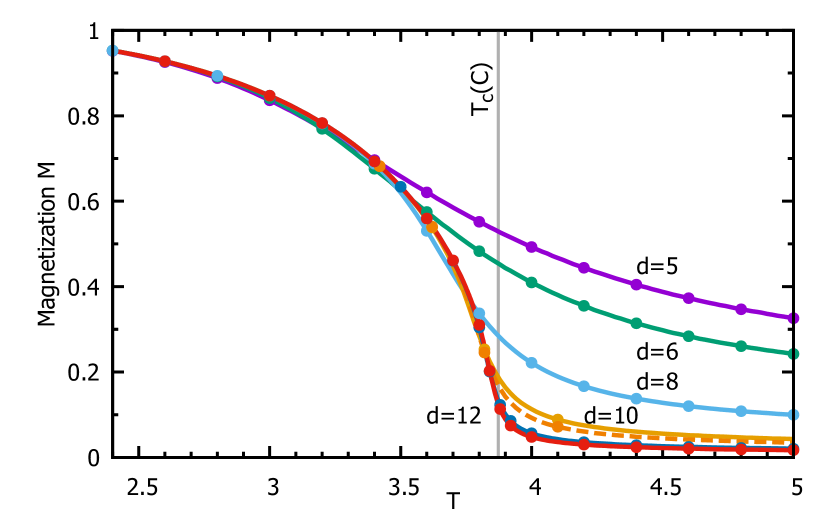
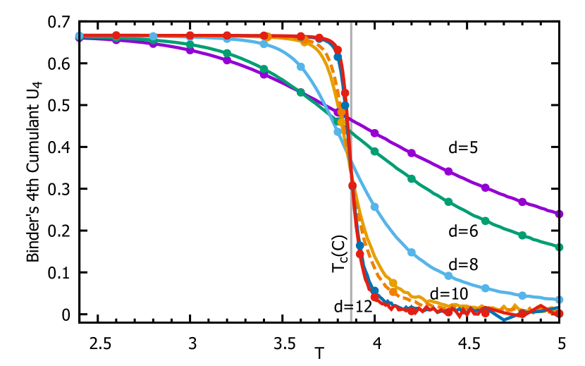
Figure 1: (Color online) Average magnetization (top) and Binder’s fourth cumulant (bottom) as a function of temperature, for transitive graphs listed in Tab. 1 with minimal distances as indicated. Dashed lines show the data for the larger $d=10$ graph. Lines show the data obtained using cluster updates; points show the data from simulations using local Metropolis updates. Vertical line shows the critical temperature $T_{c}(C)$ extrapolated from the positions of the specific heat maxima, see Fig. 5. While both sets of data do cross near $T_{c}(C)$, there is significant drift with increased graph size. In addition, the curves are near parallel which makes reliable extraction of the critical temperature difficult.

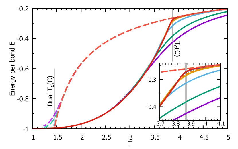
Figure 2: (Color online). Solid lines: energy per bond from Wolff cluster calculations as a function of temperature, as in Fig. 1. These data are converted with the help of the exact duality (9) to give energies in the dual model (long dashes). With increasing graph sizes, the difference between the original and dual energies decreases above the empirically found $T_{c}(C)$ (Fig. 5) and below the corresponding Kramers-Wannier dual, $T_{c}^{*}(C)$. Inset: close up of the plots near $T_{c}(C)$.

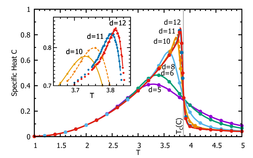
Figure 3: (Color online). As in Fig. 1 but for the specific heat. Inset: fitting for maxima. Data points in the inset are from the Wolff cluster calculations, while the lines are obtained using non-linear fits with general quartic polynomials of the form $y=y_{m}+a_{2}(x-x_{m})^{2}+\ldots+a_{4}(x-x_{m})^{4}$, which give the coordinates of the maximum $(x_{m},y_{m})$ nearly independent from the rest of the coefficients.

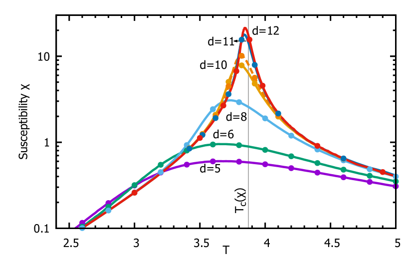
Figure 4: (Color online). As in Fig. 1 but for the susceptibility $\chi(T)$, plotted in semi logarithmic scale. The vertical line shows the critical temperature extrapolated from the susceptibility maxima, see Fig. 5.

The parameters of the graphs used in the simulations are listed in Tab. 1. The first three graphs we obtained from N. P. BreuckmannBreuckmann (2017). We generated the remaining graphs with a custom gapGAP program, which constructs coset tables of freely presented groups obtained from the infinite van Dyck group $D(5,5,2)=\langle a,b|a^{5},b^{5},(ab)^{2}\rangle$ [here $a$ and $b$ are group generators, while the remaining arguments are relators which corresponds to imposed conditions, $a^{5}=b^{5}=(ab)^{2}=1$] by adding one or more relator obtained as a pseudo random string of generators, until a finite group is obtained. Given such a finite group ${\cal D}$, the vertices, edges, and faces are enumerated by the right cosets with respect to the subgroups $\langle a\rangle$, $\langle ab\rangle$, and $\langle b\rangle$, respectively. The vertex-edge and face-edge incidence matrices $G$ and $H$ are obtained from the coset tables. Namely, non-zero matrix elements are in positions where the corresponding pair of cosets share an element. Finally, the distance $d$ of the CSS code ${\cal Q}(G,H)$ was computed using the random window algorithm, which has the advantage of being extremely fast when distance is smallDumer et al. (2014, 2017). With the exception of the graph with $n=7440$, the graphs used have the smallest size for the given distance.

vertices $r$	edges $n$	homology rank $k$	CSS distance $d$
32	80	18	5
60	150	32	6
360	900	182	8
1920	4800	962	10
2976	7440	1490	10
8640	21600	4322	11
12180	30450	6092	12

Table 1: Parameters of the graphs used in the simulations.

The obtained plots of magnetization and Binder’s fourth cumulant are shown in Fig. 1; the corresponding curves on largest graphs are nearly indistinguishable, consistent with convergence at large $n$. We note that the crossing point in the Binder’s fourth cumulant show a significant drift with the system size, see lower plot on Fig. 1. This is not surprising, given that the original scaling analysisBinder (1981) only applies to locally flat systems, whereas the hyperbolic graphs have a uniform negative curvature. On both plots, the curves for larger system sizes are near parallel to each other, which makes the identification of the phase transition point from the corresponding crossing points difficult.

Fig. 2 shows energy per bond as a function of temperature. To illustrate the properties of the specific homological difference, see Theorems 1 and 2, we also plot the energy per bond of the exact dual models obtained from the same data using $\varepsilon^{*}(K^{*})=-\sinh(2K)\,\varepsilon(K)-\cosh(2K)$, derived from Eq. (9). The plot shows that as the size of the graph increases, the difference between the energies $\varepsilon^{*}(T)$ and $\varepsilon(T)$ decreases with increasing graph size both above $T_{c}(C)$ and below the corresponding Kramers-Wannier dual, $T_{c}^{*}(C)$, while a finite difference remains for the intermediate temperatures. This is consistent with the identification $T_{h}^{*}=T_{c}(C)$.

The plots for specific heat $C(T)$ (Fig. 3) and magnetic susceptibility $\chi(T)$ (Fig. 4) show well developed maxima which become sharper and higher with increasing system sises. Notice that a unique point of divergence of the specific heat necessarily coincides with the dual homological temperature $T_{h}^{*}$.

We obtained the positions of the specific heat and magnetic susceptibility maxima by fitting the data in the vicinity of the corresponding maxima with quartic polynomials as explained in the caption of Fig. 3. The resulting positions of the maxima are plotted in Fig. 5 as a function of $x=1/n^{1/2}$. The error bars of the positions of the maxima have errors in the third digit; the observed minor scattering of the data is a feature of the corresponding graphs.

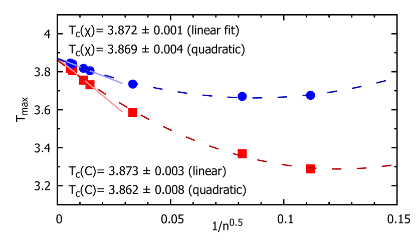
Figure 5: (Color online). Extrapolation of the specific heat and susceptibility maxima to infinite system size. Red squares (blue circles) show the positions of the specific heat (susceptibility) maxima extracted from the data on Figs. 3 and 4, respectively for graphs of different size, plotted as a function of $1/n^{1/2}$, where $n$ is the number of edges in the corresponding graphs, see Tab. 1. Solid (dashed) lines are obtained as linear (quadratic) fits to the data, where only the four leftmost points were used for the linear fits. This results in the extrapolated critical temperature values as indicated.

While the size dependence is not monotonic in the case of susceptibility maxima, the data points for larger graphs show approximately linear dependence on $x$. Linear extrapolation to infinite size ($x=0$) gives $T_{c}\approx 3.872\pm 0.003$ for both sets of data. This value is consistent with the lower bound (41) for the infinite graph with wired boundary conditions, which gives in the present case $T_{c}\geq 2.668$. In comparison, the transition for a square-lattice Ising model is in the self-dual point, $T_{\mathrm{s.d.}}=2/\ln(1+\sqrt{2})\approx 2.269$.

We note that even though we expect Ising model on hyperbolic graphs to have mean field criticality, conventional finite size scaling theory does not apply here. In particular, this is seen from the absence of the well defined crossing point in the data for Binder’s fourth cumulant, see the lower plot on Fig. 1. Therefore, we had to experiment on how to extrapolate the positions of the maxima to estimate the critical temperature. The scaling with $x=1/n^{1/2}$ was chosen since it gives near identical estimates for the critical temperatures from the maxima of $C(T)$ and $\chi(T)$, cut off at different maximum sizes (we tried $d_{\mathrm{max}}=8$ and above).

We also note that the data shows good convergence with increased system size, without the need for the subsequence construction described in Sec. III.2.

IV Discussion

IV.1 Summary of the results

We considered pairs of weakly dual Ising models with few-body couplings, defined via sequences of degree-limited bipartite coupling graphs, with the focus on the case where the rank $k$ of the first homology group of the corresponding two-chain complex scales extensively with the system size. This construction is needed to avoid introducing the boundaries, which are known to affect the position of the critical point in non-amenable graphs, and also to connect to applications, e.g., in quantum information theory, where results for large but finite systems are of interest. Here, extensive scaling of $k$ corresponds to quantum error correcting codes with finite rates $R>0$. Important examples include two-body Ising models on families of finite transitive hyperbolic graphs which weakly converge to regular $\{f,d\}$-tilings of the hyperbolic plane with $df/(d+f)>2$; the corresponding limiting rates $R=1-2/d-2/f$ are non-zero.

Our main result is Theorem 1, which guarantees the existence of a low-temperature, low-disorder region where homological defects are frozen out—in the thermodynamical limit they have no effect on the free energy density. Duality guarantees the existence of a high-temperature phase where extensive homological defects have near zero free energy cost, see Theorem 2. At all temperatures below this phase, the average defect tension is non-zero, see Eq. (31).

With the help of duality and a known bound on high-order cumulants, we established the absolute convergence of both the high- and low-temperature series expansions of the free energy density in finite regions which include vicinities of the real temperature axis around the zero and infinite temperatures, respectively. We used a subsequence construction to ensure the convergence of free energy density at all temperatures, and defined the critical temperatures as the real-axis points of non-analyticity of the limiting free energy density. For these critical temperatures, we derived several inequalities, in particular, an analog of multiplicity of the critical points, which guarantees that with $R>0$, critical point of the free energy density is affected by the summation over the topological defects.

As an application of obtained bounds, we proved the multiplicity of phase transitions on all regular tilings $\mathbf{H}(f,d)$ of the infinite hyperbolic plane, $df/(d+f)>2$.

We also simulated the phase transition on a sequence of self-dual $\{5,5\}$ transitive hyperbolic graphs without boundaries, with up to $n_{\mathrm{max}}=30450$ bonds numerically. Our data shows good convergence with increasing system sizes, with a single specific heat maximum which sharpens with the increasing system size. If the corresponding position $T_{c}(C)\approx 3.872\pm 0.003$ is the only singularity of the free energy, then necessarily it coincides with the dual homological point, $T_{h}^{*}=T_{c}(C)$.

IV.2 Open questions

1. The rightmost point of the homological region established in Theorem 1 on the $p$-$T$ plane has the same value $p_{\mathrm{max}}$ as can be also obtained using the energy-based argumentsDumer et al. (2015), which apply at $T=0$. Either of these results also impliesNishimori (2001); Kovalev and Pryadko (2015) that the portion of the Nishimori line at $p<p_{\mathrm{max}}$ is in the homological region. It should be possible to establish the existence of a homological region in the intermediate temperature points, but we could not find the corresponding arguments.

2. The proof of Statement 3 is based on overly generic boundsFéray et al. (2016) for cumulants of a sum of random variables with a given dependency graph. In the case of the Ising model, it should be possible to construct a stronger lower bound for absolute convergence of the HTS. We expect that the same bound as in Theorem 2 should apply. Such a bound would be consistent with that from high-temperature series expansions for spin correlationsFisher (1967), and it would also be consistent with the analysis of the higher-order derivatives of free energyLebowitz (1972), as well as the naive expectation that $T_{c}(G)=T_{h}^{*}(H,G)$.

3. In addition to the case in Remark 4-2, the infinite subsequence construction of Corollary 4 is also not needed when the sequence of Tanner graphs has a well defined distributional limit (Benjamini-Schramm or “left” convergenceBenjamini and Schramm (2001); Borgs et al. (2013); Lovász (2016)). Important examples are given by the Tanner graphs of hypergraph-product and related codesTillich and Zemor (2009); Kovalev and Pryadko (2013) based on specific families of sparse random matrices. For such sequences, it would be nice to establish the conditions for convergence of the free energy density or spin averages for all $K>0$, to supercede the subsequence construction of Lemma 5.

Appendix A Proof of Theorem 1

See 1

The statement of the theorem immediately follows from the following technical Lemma, see the proof in Ref. Kovalev et al., 2018

Lemma 9.

Consider a pair of Ising models defined in terms of weight-limited matrices $G$ and $H$ with orthogonal rows, such that the matrix $H$ has a maximum row weight $m$. Let $d_{G}$ denote the CSS distance (22), the minimum weight of a frustration-free homologically non-trivial defect $\mathbf{c}\in{\cal C}_{H}^{\perp}\setminus{\cal C}_{G}$. Denote $S\equiv e^{-2K}(1-p)+e^{2K}p$, and assume that $(m-1)\,S<1$. Then, the average homological difference (24) satisfies

$$[\Delta f(G,H;K)]_{p}\leq{(m-1)^{d_{G}}S^{d_{G}+1}\over 1-(m-1)\,S}.$$ (45)

Appendix B Proof of inequalities in Sec. III.1

(i) The proof of the monotonicity of the homological difference (in the absence of flipped bonds),

$${d\over dK}\Delta f_{\mathbf{0}}(G,H;K)\leq 0,$$

is similar to the proofBricmont et al. (1980) of the monotonicity of the tension. We combine the logarithms in Eq. (24), decompose $Z_{\mathbf{e}}(H^{*};K)$ as a sum of $Z_{\mathbf{c}}(G;K)$ over non-equivalent codewords $\mathbf{c}$, and write

$${d\over dK}{Z_{\mathbf{c}}(G;K)\over Z_{\mathbf{0}}(G;K)}={Z_{\mathbf{c}}(G;K)\over Z_{\mathbf{0}}(G;K)}\sum_{b\in\mathcal{B}}\left(\langle R_{b}\rangle_{\mathbf{c}}-\langle R_{b}\rangle_{\mathbf{0}}\right)\leq 0.$$

The desired inequality (26) follows from the monotonicity of the logarithm.

(ii) The first inequality in

$$|\tau_{\mathbf{c,e}}|\leq\tau_{\mathbf{c,0}}\leq 2K$$

follows from the second GKS inequalityGriffiths (1967); Kelly and Sherman (1968) applied in the dual system [where, according to electric-magnetic duality, the defect becomes an average of the corresponding product of spins, see Eq. (11)]. Depending on the sign of $\tau_{\textbf{c,e}}$, duality gives $\langle R_{\mathbf{c+e}}\rangle\geq\langle R_{\mathbf{e}}\rangle\langle R_{\mathbf{c}}\rangle$ or $\langle R_{\mathbf{e}}\rangle\geq\langle R_{\mathbf{c}}\rangle\langle R_{\mathbf{e+\mathbf{c}}}\rangle$, where $R_{\mathbf{e}}$ is the product of bonds corresponding to non-zero bits in the binary vector $\mathbf{e}$. The second inequality, in a more general form, $\tau_{\mathbf{e}}\equiv\tau_{\mathbf{e,0}}\leq 2K$, follows from the Gibbs inequality

$$F_{\mathbf{e}}(G;K)-F_{\mathbf{0}}(G;K)\leq 2K\sum_{b:e_{b}\neq 0}\langle R_{b}\rangle_{G;K}\leq 2K\mathop{\rm wgt}(\mathbf{e}),$$

if we take a minimal-weight vector equivalent to $\mathbf{e}$, in which case $\mathop{\rm wgt}(\mathbf{e})=d_{\mathbf{e}}$.

(iii) To prove the lower bound on the average tension,

$$\zeta\bar{\tau}_{p}\geq R\ln 2-[\Delta f_{\mathbf{e}}]_{p},$$

we first define the constant $\zeta$ as the average minimum weight of all $2^{k}$ codewords divided by the code length $n$,

$$\zeta=(2^{k}n)^{-1}\sum_{\mathbf{c}}d_{\mathbf{c}}.$$ (46)

An upper bound on $\zeta$ can be obtained if we take the codewords $\mathbf{c}$ as linear combinations of $k$ inequivalent codewords $\mathbf{c}_{i}$, $i\in\{1,\ldots,k\}$ (it is likely that smaller-weight equivalent codewords can be found). In this case the codewords form a binary code, and the average weight is exactly a half of the length $n^{\prime}$ of the codeMacWilliams and Sloane (1981), where $n^{\prime}=\left|\cup_{i=1}^{k}I({\bf c}_{i})\right|$ is the weight of the union of the supports of the basis codewords. Clearly, $n^{\prime}\leq n$, which gives $\zeta\leq 1/2$. Combining with a lower bound on the weight of non-trivial codewords, $d_{\mathbf{c}}\geq d_{\cal G}$, $\mathbf{c}\not\simeq\mathbf{0}$, we obtain

$${1-2^{-k}\over n}d_{G}\leq\zeta\leq{1\over 2}.$$ (47)

We now proceed with deriving the inequality (31). Start by expanding $Z_{\mathbf{e}}(H^{*};K)=\sum_{\mathbf{c}}Z_{\mathbf{e+c}}(G;K)$, where the summation is over all $2^{k}$ mutually inequivalent codewords $\mathbf{c}$. Each of the terms with $\mathbf{c}\not\simeq\mathbf{0}$ can be written in terms of the corresponding tension (28),

$$Z_{\mathbf{e+c}}(G;K)=e^{-\tau_{\mathbf{c,e}}(G;K)d_{\mathbf{c}}}Z_{\mathbf{e}}(G;K).$$

Convexity of the exponent gives

$${Z_{\mathbf{e}}(H^{*};K)\over Z_{\mathbf{e}}(G;K)} = 1+\sum_{\mathbf{c\not\simeq 0}}\exp(-\tau_{\mathbf{c,e}}d_{c})$$

$$\geq 2^{k}\exp\Biglb(-{2^{-k}}\sum_{\mathbf{c}}\tau_{\bf c,e}d_{\mathbf{c}}\Bigrb),$$

where for the trivial codeword $\mathbf{c}\simeq\mathbf{0}$ we set $\tau_{\bf 0,e}d_{\mathbf{0}}=0$. Taking the logarithm and rewriting the sum over codewords in terms of the weighted average, with the help of Eq. (46) we obtain

$$\Delta F_{\mathbf{e}}(G,H;K)\geq k\ln 2-\zeta n{\sum_{\mathbf{c\not\simeq 0}}\tau_{\mathbf{c,e}}d_{\mathbf{c}}\over\sum_{\mathbf{c\not\simeq 0}}d_{\mathbf{c}}}.$$

Eq. (31) trivially follows after averaging over disorder and dividing by $n$.

(iv) The inequality

$$K_{h}(G,H)-K_{h}^{*}(H,G)\geq R\ln 2$$

is based on the standard inequality for the derivative of the free energy density, which is just the average energy per bond. For the case of homological difference we obtain, instead,

$${d\over dK}\Delta f(G,H;K)={1\over n}\sum_{b\in\mathcal{B}}\left(\langle R_{b}\rangle_{H^{*};K}-\langle R_{b}\rangle_{G;K}\right).$$ (48)

The second term can be obtained from the first by freezing the spins corresponding to homologically non-trivial defects; with the help of GKS inequalities we obtain

$$1\geq\langle R_{b}\rangle_{G;K}\geq\langle R_{b}\rangle_{H^{*};K}\geq 0,$$

which guarantees the derivative (48) to be between $-1$ and $0$. Integration gives the inequality

$$\Delta f_{t}(K_{2})-\Delta f_{t}(K_{1})\leq K_{1}-K_{2},$$

where $\Delta f_{t}(K)=\Delta f(G_{t},H_{t};K)$. We now take $K_{1}=K_{h}(G,H)$ and $K_{2}=K_{h}^{*}(H,G)$, so that in the limit of the sequence, $\lim_{t}\Delta f_{t}(K_{1})=0$ and $\lim_{t}\Delta f_{t}(K_{2})=R\ln 2$. Eq. (34) trivially follows.

Appendix C Proof of Theorem 2

See 2

Proof.

The proof is based on the special case of Theorem 1 in the absence of disorder, $p=0$, and the duality relation (32), applied for each pair of matrices, $G_{t}$ and $H_{t}$, with $R_{t}=k_{t}/n_{t}$, and $K$ replaced with its Kramers-Wannier dual, $K^{*}$. The condition on $K$ in Theorem 1 (with $G_{t}$ and $H_{t}$ interchanged) becomes simply $(m-1)\tanh K<1$. Convergence of sequences $\Delta f_{\mathbf{0}}(H_{t},G_{t};K^{*})$ to $0$ and $R_{t}$ to $R$ implies that of the sequence $\Delta f_{\mathbf{0}}(G_{t},H_{t};K)$ to $R\ln 2$. ∎

Appendix D Proof of Statement 3

The proof is based on Theorem 9.1.7 from Ref. Féray et al., 2016, which bounds cumulants of a random variable $X$,

$$\kappa_{r}(X)\equiv{d^{r}\over dt^{r}}\,\ln\mathbb{E}\left(e^{tX}\right)\biggr{|}_{t=0},\;\,r\in\{0,1,\ldots\},$$ (49)

where $X=\sum_{\alpha\in{\cal S}}Y_{\alpha}$ is a sum of random variables with a given dependency graph:

Definition 1.

A graph ${\cal D}$ with vertex set ${\cal S}$ is called a dependency graph for the set of random variables $\{Y_{\alpha},\alpha\in{\cal S}\}$ if for any two disjoint subsets ${\cal S}_{1}$ and ${\cal S}_{2}$ of ${\cal S}$, such that there are no edges in ${\cal D}$ connecting an element of ${\cal S}_{1}$ and an element of ${\cal S}_{2}$, the sets of random variables $\{Y_{\alpha}\}_{\alpha\in{\cal S}_{1}}$ and $\{Y_{\alpha}\}_{\alpha\in{\cal S}_{2}}$ are independent.

The corresponding bound reads as follows:

Lemma 10 (Theorem 9.1.7 from Ref. Féray et al., 2016).

Let $\{Y_{\alpha}\}_{\alpha\in{\cal S}}$ be a family of random variables with dependency graph ${\cal D}$. Denote $N=|{\cal S}|$ the number of vertices of ${\cal D}$ and $\Delta$ the maximal degree of ${\cal D}$. Assume that the variables $Y_{\alpha}$ are uniformly bounded by a constant $A$. Then, for the sum $X=\sum_{\alpha\in{\cal S}}Y_{\alpha}$, and for any $s\in\{0,1,\ldots\}$, one has

$$|\kappa_{s}(X)|\leq 2^{s-1}s^{s-2}N(\Delta+1)^{s-1}A^{s}.$$ (50)

See 3

Proof of Statement 3 .

The $s$-th coefficient of the HTS for the free energy $F(\Theta;K,h)$ is the scaled cumulant $-\kappa_{s}(X)/s!$, where $X=J\sum_{b\in{\cal B}}R_{b}+h^{\prime}\sum_{v\in{\cal V}}S_{v}$. Define the set of random variables $Y_{\alpha}$ as the union of the set of (scaled) spins $hS_{v}$ and bonds $KR_{b}$, then $|Y_{\alpha}|\leq A\equiv\max(|h^{\prime}|,|J|)$. The corresponding dependency graph ${\cal D}$ can be obtained from the bipartite graph defined by the matrix $\Theta$ by connecting any pair of nodes for bonds which share the same spin. In the original bipartite graph, each spin node has up to $\ell$ neighboring bond nodes, and each bond node has up to $m$ neighboring spin nodes. In the modified graph, each bond node also connects with up to $(\ell-1)m$ bond nodes with common spins, which gives the total maximum degree of $\Delta=\ell m$. We also have $N=|{\cal V}|+|{\cal E}|=r+n$, dividing by $n$ as appropriate for the free energy density we obtain the bound in part (a). With $h=0$, we can drop the spin nodes from the dependency graph. In this case the maximum degree is $\Delta^{\prime}=(\ell-1)m$, which gives the result in part (b). Notice that in this case $N=n$, and the factor $C=(r/n+1)$ is replaced with $C^{\prime}=1$. ∎

Appendix E Proof of Corollary 4.

See 4

Proof.

The result in Statement 3(b) gives a uniform in $t$ bound on the coefficients of the HTS,

$${|\kappa_{s}(\Theta_{j})|\over s!} \leq {2^{s-1}s^{s-2}(\Delta+1)^{s-1}J^{s}\over(2\pi s)^{1/2}(s/e)^{s}}$$ (51)

$$= {1\over\sqrt{8\pi}(\Delta+1)}{[2eJ\,(\Delta+1)]^{s}\over s^{5/2}},$$

where $\Delta\equiv(\ell-1)m$ and we used the lower bound by Stirling, $r!\geq(2\pi r)^{1/2}(r/e)^{r}$. The bound (51) is uniform in the sequence index $j\in\mathbb{N}$. Thus one can select an infinite subsequence of ${\Theta}_{j}$, ${\Theta}_{j^{\prime}(t)}$, $t\in\mathbb{N}$, where the function $j^{\prime}:\mathbb{N}\to\mathbb{N}$ is strictly increasing, so that the coefficients $\kappa_{m}(\Theta_{j^{\prime}(t)})$ for $m=1$ converge with $t$. Selecting an infinite subsequence of the one obtained previously to ensure the convergence of the coefficients $\kappa_{m}$ for $m=2,3,\ldots$, at each step we obtain an infinite subsequence such that all coefficients $\kappa_{s}$ with $s\leq m$ converge with $t$. The statement in part (a) is obtained in the limit of $m\to\infty$. The uniform bound (51) also applies to the cumulants after we take the limit of the obtained subsequence, which implies absolute convergence (and thus analyticity of the limit) of the HTS for free energy density in the circle $|K|\equiv|\beta|J\leq\{2e[(\ell-1)m+1]\}^{-1}$, which is exactly the statement in part (b). ∎

Appendix F Proof of Lemma 5

See 5

Proof.

For any $t$, the free energy density $f_{t}(K)=-n_{t}^{-1}\ln Z_{\mathbf{0}}(G_{t},K)$ is bounded from both sides,

$$-M\leq r_{t}\ln 2/n_{t}-K\leq f_{t}(K)\leq r_{t}\ln 2/n_{t}+K\leq\ln 2+M.$$

Therefore, we can use a subsequence construction to ensure convergence in any point $K\in I_{M}$. Since the set of rational numbers $\mathbb{Q}$ is countable, we can repeat this construction sequentially on all rational points in $I_{M}$. The resulting infinite sequence $f_{i}(K)$ converges in any rational point $K\in I_{M}\cap\mathbb{Q}$. Further, the derivative of $f_{i}(K)$ is uniformly bounded, $-1\leq f_{i}^{\prime}(K)\leq 0$. Since the sequence converges on a dense subset of $I_{M}$, this guarantees the existence and the continuity of the limit in the entire interval. Finally, each of $f_{i}(K)$ is concave and non-increasing; these properties survive the limit, although the resulting function may not necessarily be strictly concave. Concavity guarantees the existence of one-sided derivatives. The lower and upper bounds on these derivatives are inherited from those for $f_{i}^{\prime}(K)$. ∎

Appendix G Proof of Theorem 6

See 6

Proof.

There are three mutually exclusive possibilities: (a) $T_{c}^{\prime}(G)<T_{h}(G,H)$, (b) $T_{c}^{\prime}(G)>T_{h}(G,H)$, and (c) $T_{c}^{\prime}(G)=T_{h}(G,H)$. In the case (a), $T_{c}^{*}(H)=T_{c}^{\prime}(G)$, since the functions $f_{G}(K)$ and $f_{H^{*}}(K)$ coincide in the homological region, i.e., for $K>K_{h}(G,H)$; Eq. (40) is satisfied. In the case (b), $T_{c}^{*}(H)=T_{h}(G,H)$, in order to recover the non-analyticity point for the homological difference; Eq. (40) is saturated. The goal of the Conditions is to deal with the case (c) which implies $T_{c}^{*}(H)\geq T_{h}(G,H)$; a strict inequality would violate Eq. (40). In the following we assume (c).

Condition 1 implies that the (negative) curvature of $f_{G}(K)$ must diverge at $K_{h}=K_{c}^{\prime}(G)$, which must be compensated by a divergent curvature of $f_{H^{*}}(K)$ in order to make $\Delta f(K)$ strictly convex in this point. In this case $T_{c}^{*}(H)=T_{c}^{\prime}(G)$; Eq. (40) is saturated.

Condition 2 does the same, since divergent positive curvature of $\Delta f(K)$ at $K_{h}$ can only come from $f_{H^{*}}(K)$.

Condition 3 is equivalent by duality to $T_{c}^{\prime}(G)\geq T_{c}^{*}(H)$, which again gives Eq. (40) since we assumed (c). ∎

Appendix H Proof of the lower bound for tension

On an infinite locally planar transitive graph $\mathcal{G}$, we would like to prove the following bound for the asymptotic defect tension (42),

$${d\tau(K)\over dK}\geq 2[m(K)]^{2},$$ (52)

the same inequality as has been previously proved on $\mathbb{Z}^{D}$ in Ref. Lebowitz and Pfister, 1981. This inequality is a trivial consequence of the following Lemma, which gives a version of Eq. (7) from Ref. Lebowitz and Pfister (1981) suitable to constructing a bound for the defect tension defined by Eq. (15).

Lemma 11.

Let $\mathcal{G}=(\mathcal{V},\mathcal{E})$ be a finite transitive graph, and $G$ the corresponding vertex-edge incidence matrix with $n=|\mathcal{E}|$ columns. Take a binary vector $\mathbf{e}\in\mathbb{F}_{2}^{n}$ selecting a set of edges $\mathcal{E}_{\mathbf{e}}\subset\mathcal{E}$ of size $|\mathcal{E}_{\mathbf{e}}|=\mathop{\rm wgt}(\mathbf{e})$, and a set of vertices $\mathcal{A}\subset\mathcal{V}$ of twice the size, $|\mathcal{A}|=2\mathop{\rm wgt}(\mathbf{e})$, such that the graph contains edge-disjoint paths connecting each edge to exactly two vertices in ${\cal A}$. Then for the Ising model defined on the same graph, at any $K,h\geq 0$, the free energy increment $\delta_{\mathbf{e}}(K)\equiv F_{\mathbf{e}}(G;K,h)-F_{\mathbf{0}}(G;K,h)$ associated with the defect $\mathbf{e}$ satisfies

$${d\delta_{\mathbf{e}}(K)\over dK}\geq\langle S_{i}\rangle_{\mathbf{0}}\sum_{v\in\mathcal{A}}\langle S_{v}\rangle_{\mathbf{e}},$$ (53)

where the average $\langle S_{v}\rangle_{\mathbf{e}}$ is calculated in the presence of the defect $\mathbf{e}$; by transitivity $\langle S_{i}\rangle_{\mathbf{0}}$ is independent of $i\in\mathcal{V}$.

Proof.

The proof is based on two inequalities,

$$\langle S_{\cal A}S_{\cal B}\rangle_{\mathbf{0}}\pm\langle S_{\cal A}S_{\cal B}\rangle_{\mathbf{e}}\geq\left|\langle S_{\cal A}\rangle_{\mathbf{0}}\langle S_{\cal B}\rangle_{\mathbf{e}}\pm\langle S_{\cal A}\rangle_{\mathbf{e}}\langle S_{\cal B}\rangle_{0}\right|,$$ (54)

where ${\cal A}\subset{\cal V}$ and ${\cal B}\subset{\cal V}$ are sets of vertices. The inequality with the lower (negative) signs is the Lebowitz comparison inequalityLebowitz (1977), while the inequality with the upper signs can be proved using the same technique. In the case of an Ising model on a graph ${\cal G}=({\cal V},{\cal E})$, we have

$${d\delta_{\mathbf{e}}(K)\over dK}=\sum_{ij=b\in{\cal E}}\left[\langle S_{i}S_{j}\rangle_{\mathbf{0}}-(-1)^{e_{b}}\langle S_{i}S_{j}\rangle_{\mathbf{e}}\right].$$

Applying Eq. (54) for each term separately, with the help of transitivity, $\langle S_{i}\rangle_{\mathbf{0}}\equiv m_{0}\geq 0$, $i\in{\cal V}$, one gets

$${d\delta_{\mathbf{e}}(K)\over dK}\geq m_{0}\sum_{b=ij\in{\cal E}}|m_{i}^{\prime}-(-1)^{e_{b}}m_{j}^{\prime}|,$$ (55)

where $m_{i}^{\prime}\equiv\langle S_{i}\rangle_{\mathbf{e}}$. The statement of the Lemma is obtained by noticing that for a path connecting $1$ and $f$,

$$|m_{1}^{\prime}-m_{2}^{\prime}|+|m_{2}^{\prime}-m_{3}^{\prime}|+\ldots+|m^{\prime}_{f-1}-m^{\prime}_{f}|\geq m^{\prime}_{f}-m_{1}^{\prime},$$

which allows to trade $\mathop{\rm wgt}({\bf e})$ terms with $+$ signs in the r.h.s. of Eq. (55) for the sum of magnetizations $m_{v}^{\prime}$ on the $2\mathop{\rm wgt}(\mathbf{e})$ vertices from ${\cal A}$. ∎

References

- Griffiths (1972) R. Griffiths, “Rigorous results and theorems,” in Phase Transitions and Critical Phenomena, Vol. 1. Exact results, edited by C. Domb and M. S. Green (Acad. Press, London, 1972) Chap. 2, pp. 7–109.
- Lebowitz (1977) Joel L. Lebowitz, “Coexistence of phases in Ising ferromagnets,” Journal of Statistical Physics 16, 463–476 (1977).
- Gruber and Lebowitz (1978) C. Gruber and J. L. Lebowitz, “On the equivalence of different order parameters and coexistence of phases for Ising ferromagnet. II,” Communications in Mathematical Physics 59, 97–108 (1978).
- Lebowitz and Pfister (1981) J. L. Lebowitz and C. E. Pfister, “Surface tension and phase coexistence,” Phys. Rev. Lett. 46, 1031–1033 (1981).
- Lyons (1989) Russell Lyons, “The Ising model and percolation on trees and tree-like graphs,” Communications in Mathematical Physics 125, 337–353 (1989).
- Lyons (2000) Russell Lyons, “Phase transitions on nonamenable graphs,” Journal of Mathematical Physics 41, 1099–1126 (2000), math/9908177 .
- Birrel and Davies (1982) N. B. Birrel and P. C. W. Davies, Quantum fields in curved space. (Cambridge University Press, Cambridge, UK, 1982).
- Cognola et al. (1993) Guido Cognola, Klaus Kirsten, and Sergio Zerbini, “One-loop effective potential on hyperbolic manifolds,” Phys. Rev. D 48, 790–799 (1993).
- Camporesi (1991) Roberto Camporesi, “-function regularization of one-loop effective potentials in anti-de sitter spacetime,” Phys. Rev. D 43, 3958–3965 (1991).
- Miele and Vitale (1997) Gennaro Miele and Patrizia Vitale, “Three-dimensional Gross-Neveu model on curved spaces,” Nuclear Physics B 494, 365 – 387 (1997).
- Doyon (2003) Benjamin Doyon, “Two-point correlation functions of scaling fields in the Dirac theory on the Poincaré disk,” Nuclear Physics B 675, 607 – 630 (2003).
- Evenbly and Vidal (2011) G. Evenbly and G. Vidal, “Tensor network states and geometry,” Journal of Statistical Physics 145, 891–918 (2011).
- Matsueda et al. (2013) Hiroaki Matsueda, Masafumi Ishihara, and Yoichiro Hashizume, “Tensor network and a black hole,” Phys. Rev. D 87, 066002 (2013).
- Nelson (1983) David R. Nelson, “Order, frustration, and defects in liquids and glasses,” Phys. Rev. B 28, 5515–5535 (1983).
- Tarjus et al. (2005) G. Tarjus, S. A. Kivelson, Z. Nussinov, and P. Viot, “The frustration-based approach of supercooled liquids and the glass transition: a review and critical assessment,” Journal of Physics: Condensed Matter 17, R1143 (2005).
- Vitelli et al. (2006) Vincenzo Vitelli, J. B. Lucks, and D. R. Nelson, “Crystallography on curved surfaces,” Proceedings of the National Academy of Sciences 103, 12323–12328 (2006).
- Sausset and Tarjus (2007) F. Sausset and G. Tarjus, “Periodic boundary conditions on the pseudosphere,” Journal of Physics A: Mathematical and Theoretical 40, 12873 (2007).
- Giomi and Bowick (2007) Luca Giomi and Mark Bowick, “Crystalline order on riemannian manifolds with variable gaussian curvature and boundary,” Phys. Rev. B 76, 054106 (2007).
- Turner et al. (2010) Ari M. Turner, Vincenzo Vitelli, and David R. Nelson, “Vortices on curved surfaces,” Rev. Mod. Phys. 82, 1301–1348 (2010).
- Garcia et al. (2015) Nicolas A. Garcia, Aldo D. Pezzutti, Richard A. Register, Daniel A. Vega, and Leopoldo R. Gomez, “Defect formation and coarsening in hexagonal 2D curved crystals,” Soft Matter 11, 898–907 (2015).
- Benedetti (2015) Dario Benedetti, “Critical behavior in spherical and hyperbolic spaces,” Journal of Statistical Mechanics: Theory and Experiment 2015, P01002 (2015).
- Cohen et al. (2000) Reuven Cohen, Keren Erez, Daniel ben-Avraham, and Shlomo Havlin, “Resilience of the internet to random breakdowns,” Phys. Rev. Lett. 85, 4626–4628 (2000).
- Albert and Barabási (2002) R. Albert and A.-L. Barabási, “Statistical mechanics of complex networks,” Rev. Mod. Phys. 74, 47–97 (2002).
- Gai and Kapadia (2010) Prasanna Gai and Sujit Kapadia, “Contagion in financial networks,” Proc. Royal Soc. A: Math., Phys. and Eng. Sci. 466, 2401–2423 (2010).
- Börner et al. (2007) K. Börner, S. Sanyal, and A. Vespignani, “Network science,” Annual Review of Information Science and Technology 41, 537–607 (2007).
- Sander et al. (2002) L. M. Sander, C. P. Warren, I. M. Sokolov, C. Simon, and J. Koopman, “Percolation on heterogeneous networks as a model for epidemics,” Mathematical Biosciences 180, 293 – 305 (2002).
- da Fontoura Costa et al. (2011) L. da Fontoura Costa, O. N. Oliveira, G. Travieso, F. A. Rodrigues, P. R. Villas Boas, L. Antiqueira, M. P. Viana, and L. E. Correa Rocha, “Analyzing and modeling real-world phenomena with complex networks: a survey of applications,” Advances in Physics 60, 329–412 (2011).
- Danon et al. (2011) L. Danon, A. P. Ford, T. House, C. P. Jewell, M. J. Keeling, G. O. Roberts, J. V. Ross, and M. C. Vernon, “Networks and the epidemiology of infectious disease,” Interdisciplinary Perspectives on Infectious Diseases 2011, 284909 (2011).
- Dennis et al. (2002) E. Dennis, A. Kitaev, A. Landahl, and J. Preskill, “Topological quantum memory,” J. Math. Phys. 43, 4452 (2002).
- Kovalev and Pryadko (2015) A. A. Kovalev and L. P. Pryadko, “Spin glass reflection of the decoding transition for quantum error-correcting codes,” Quantum Inf. & Comp. 15, 0825 (2015), arXiv:1311.7688 .
- Kovalev et al. (2018) Alexey A. Kovalev, Sanjay Prabhakar, Ilya Dumer, and Leonid P. Pryadko, “Numerical and analytical bounds on threshold error rates for hypergraph-product codes,” (2018), unpublished, 1804.01950 .
- Wu (2000) C. Chris Wu, “Ising models on hyperbolic graphs II,” Journal of Statistical Physics 100, 893–904 (2000).
- Schonmann (2001) H. Roberto Schonmann, “Multiplicity of phase transitions and mean-field criticality on highly non-amenable graphs,” Communications in Mathematical Physics 219, 271–322 (2001).
- Häggström et al. (2002) Olle Häggström, Johan Jonasson, and Russell Lyons, “Explicit isoperimetric constants and phase transitions in the random-cluster model,” Ann. Probab. 30, 443–473 (2002).
- Wegner (1971) F. Wegner, “Duality in generalized Ising models and phase transitions without local order parameters,” J. Math. Phys. 2259, 12 (1971).
- Tanner (1981) R. Tanner, “A recursive approach to low complexity codes,” IEEE Trans. Info. Th. 27, 533–547 (1981).
- Percus (1975) J. K. Percus, “Correlation inequalities for Ising spin lattices,” Communications in Mathematical Physics 40, 283–308 (1975).
- Shlosman (1981) S. B. Shlosman, “Correlation inequalities and their applications,” Journal of Soviet Mathematics 15, 79–101 (1981).
- Griffiths (1967) Robert B. Griffiths, “Correlations in Ising ferromagnets. I,” J. Math. Phys. 8, 478 (1967).
- Kelly and Sherman (1968) D. G. Kelly and S. Sherman, “General Griffiths’ inequalities on correlations in Ising ferromagnets,” Journal of Mathematical Physics 9, 466–484 (1968).
- Kramers and Wannier (1941) H. A. Kramers and G. H. Wannier, “Statistics of two-dimensional ferromagnet. Part I,” Phys. Rev. 60, 252–262 (1941).
- Nishimori (2001) Hidetoshi Nishimori, Statistical Physics of Spin Glasses and Information Processing: An Introduction (Clarendon Press, Oxford, 2001).
- Gottesman (1997) Daniel Gottesman, Stabilizer Codes and Quantum Error Correction, Ph.D. thesis, Caltech (1997).
- Calderbank et al. (1998) A. R. Calderbank, E. M. Rains, P. M. Shor, and N. J. A. Sloane, “Quantum error correction via codes over GF(4),” IEEE Trans. Info. Theory 44, 1369–1387 (1998).
- Nielsen and Chuang (2000) M. A. Nielsen and I. L. Chuang, Quantum Computation and Quantum Infomation (Cambridge Unive. Press, Cambridge, MA, 2000).
- Preskill (2000) John Preskill, Course Information for Physics 219/Computer Science 219 Quantum Computation (Caltech, 2000).
- Calderbank and Shor (1996) A. R. Calderbank and P. W. Shor, “Good quantum error-correcting codes exist,” Phys. Rev. A 54, 1098–1105 (1996).
- Steane (1996) A. M. Steane, “Simple quantum error-correcting codes,” Phys. Rev. A 54, 4741–4751 (1996).
- Note (1) Notice that any other construction of the dual matrix would at most change the partition function multiplicatively by a power of two.
- Féray et al. (2016) Valentin Féray, Pierre-Loïc Méliot, and Ashkan Nikeghbali, Mod- convergence I: Normality zones and precise deviations (Springer International Publishing, Cham, 2016) arXiv:1304.2934v4 .
- Benjamini and Schramm (2001) I. Benjamini and O. Schramm, “Recurrence of distributional limits of finite planar graphs,” Electron. J. Probab. 6, 23/1–13 (2001), math/0011019 .
- Borgs et al. (2013) Christian Borgs, Jennifer Chayes, Jeff Kahn, and László Lovász, “Left and right convergence of graphs with bounded degree,” Random Structures & Algorithms 42, 1–28 (2013), 1002.0115 .
- Lovász (2016) L. M. Lovász, “A short proof of the equivalence of left and right convergence for sparse graphs,” Eur. J. Comb. 53, 1–7 (2016).
- Domb and Green (1974) C. Domb and M. S. Green, eds., Phase transitions and critical phenomena, Vol. 3 (Academic, London, 1974).
- Bravyi and Terhal (2009) Sergey Bravyi and Barbara Terhal, “A no-go theorem for a two-dimensional self-correcting quantum memory based on stabilizer codes,” New Journal of Physics 11, 043029 (2009).
- Bravyi et al. (2010) S. Bravyi, D. Poulin, and B. Terhal, “Tradeoffs for reliable quantum information storage in 2D systems,” Phys. Rev. Lett. 104, 050503 (2010), 0909.5200 .
- Tillich and Zemor (2009) J.-P. Tillich and G. Zemor, “Quantum LDPC codes with positive rate and minimum distance proportional to ,” in Proc. IEEE Int. Symp. Inf. Theory (ISIT) (2009) pp. 799–803.
- Kovalev and Pryadko (2013) A. A. Kovalev and L. P. Pryadko, “Quantum Kronecker sum-product low-density parity-check codes with finite rate,” Phys. Rev. A 88, 012311 (2013).
- Guth and Lubotzky (2014) Larry Guth and Alexander Lubotzky, “Quantum error correcting codes and 4-dimensional arithmetic hyperbolic manifolds,” Journal of Mathematical Physics 55, 082202 (2014), arXiv:1310.5555 .
- Montanari et al. (2012) Andrea Montanari, Elchanan Mossel, and Allan Sly, “The weak limit of Ising models on locally tree-like graphs,” Probability Theory and Related Fields 152, 31–51 (2012).
- Širáň (2001) Jozef Širáň, “Triangle group representations and constructions of regular maps,” Proceedings of the London Mathematical Society 82, 513–532 (2001).
- Delfosse and Zémor (2010) N. Delfosse and G. Zémor, “Quantum erasure-correcting codes and percolation on regular tilings of the hyperbolic plane,” in Information Theory Workshop (ITW), 2010 IEEE (2010) pp. 1–5.
- Delfosse and Zémor (2013) N. Delfosse and G. Zémor, “Upper bounds on the rate of low density stabilizer codes for the quantum erasure channel,” Quantum Info. Comput. 13, 793–826 (2013), 1205.7036 .
- Delfosse (2013) Nicolas Delfosse, “Tradeoffs for reliable quantum information storage in surface codes and color codes,” in Information Theory Proceedings (ISIT), 2013 IEEE International Symposium on (IEEE, 2013) pp. 917–921.
- Delfosse and Zémor (2016) N. Delfosse and G. Zémor, “A homological upper bound on critical probabilities for hyperbolic percolation,” Ann. Inst. Henri Poincaré Comb. Phys. Interact. 3, 139–161 (2016), 1408.4031 .
- Breuckmann and Terhal (2015) N. P. Breuckmann and B. M. Terhal, “Constructions and noise threshold of hyperbolic surface codes,” (2015), unpublished, 1506.04029 .
- Breuckmann et al. (2017) Nikolas P. Breuckmann, Christophe Vuillot, Earl Campbell, Anirudh Krishna, and Barbara M. Terhal, “Hyperbolic and semi-hyperbolic surface codes for quantum storage,” Quantum Science and Technology 2, 035007 (2017).
- Breuckmann (2017) Nikolas P. Breuckmann, Homological Quantum Codes Beyond the Toric Code, Ph.D. thesis, RWTH Aachen University (2017), 1802.01520 .
- Kitaev (2003) A. Yu. Kitaev, “Fault-tolerant quantum computation by anyons,” Ann. Phys. 303, 2 (2003).
- Metropolis et al. (1953) Nicholas Metropolis, Arianna W. Rosenbluth, Marshall N. Rosenbluth, Augusta H. Teller, and Edward Teller, “Equation of state calculations by fast computing machines,” The Journal of Chemical Physics 21, 1087–1092 (1953).
- Wolff (1989) Ulli Wolff, “Collective monte carlo updating for spin systems,” Phys. Rev. Lett. 62, 361–364 (1989).
- Binder (1981) K. Binder, “Finite size scaling analysis of Ising model block distribution functions,” Zeitschrift für Physik B Condensed Matter 43, 119–140 (1981).
- (73) GAP, GAP – Groups, Algorithms, and Programming, Version 4.8.10, The GAP Group (2018).
- Dumer et al. (2014) I. Dumer, A. A. Kovalev, and L. P. Pryadko, “Numerical techniques for finding the distances of quantum codes,” in Information Theory Proceedings (ISIT), 2014 IEEE International Symposium on (IEEE, Honolulu, HI, 2014) pp. 1086–1090.
- Dumer et al. (2017) I. Dumer, A. A. Kovalev, and L. P. Pryadko, “Distance verification for classical and quantum LDPC codes,” IEEE Trans. Inf. Th. 63, 4675–4686 (2017).
- Dumer et al. (2015) I. Dumer, A. A. Kovalev, and L. P. Pryadko, “Thresholds for correcting errors, erasures, and faulty syndrome measurements in degenerate quantum codes,” Phys. Rev. Lett. 115, 050502 (2015), 1412.6172 .
- Fisher (1967) Michael E. Fisher, “Critical temperatures of anisotropic Ising lattices. II. General upper bounds,” Phys. Rev. 162, 480–485 (1967).
- Lebowitz (1972) Joel L. Lebowitz, “Bounds on the correlations and analyticity properties of ferromagnetic Ising spin systems,” Communications in Mathematical Physics 28, 313–321 (1972).
- Bricmont et al. (1980) Jean Bricmont, Joel L. Lebowitz, and Charles E. Pfister, “On the surface tension of lattice systems,” Annals of the New York Academy of Sciences 337, 214–223 (1980).
- MacWilliams and Sloane (1981) F. J. MacWilliams and N. J. A. Sloane, The Theory of Error-Correcting Codes (North-Holland, Amsterdam, 1981).