Privacy preserving distributed optimization using homomorphic encryption

Abstract

This paper studies how a system operator and a set of agents securely execute a distributed projected gradient-based algorithm. In particular, each participant holds a set of problem coefficients and/or states whose values are private to the data owner. The concerned problem raises two questions: how to securely compute given functions; and which functions should be computed in the first place. For the first question, by using the techniques of homomorphic encryption, we propose novel algorithms which can achieve secure multiparty computation with perfect correctness. For the second question, we identify a class of functions which can be securely computed. The correctness and computational efficiency of the proposed algorithms are verified by two case studies of power systems, one on a demand response problem and the other on an optimal power flow problem.

AND

,

1 Introduction

In the last decades, distributed optimization has been extensively studied and broadly applied to coordinate large-scale networked systems Bertsekas and Tsitsiklis (1997), Zhu and Martínez (2015), Bullo et al. (2009). In distributed optimization, the participants collectively achieve network-wide goals via certain mechanisms driven by data sharing between the participants. Such data sharing, however, causes the concern that private information of legitimate entities could be leaked to unauthorized ones. Hence, there is a demand to develop new distributed optimization algorithms that can achieve network-wide goals and simultaneously protect the privacy of legitimate entities.

The problem of interest is closely relevant to the one where a group of participants aim to compute certain functions over their distributed private inputs such that each participant’s inputs remain private after the computation. To protect privacy, two questions need to be answered Lindell and Pinkas (2009): (i) How to securely compute given functions with distributed private inputs so that the computation process does not reveal anything beyond the function outputs? This question is referred to as secure multiparty computation (SMC) Hazay and Lindell (2010), Cramer et al. (2015). (ii) Which functions should be computed in the first place so that the adversary cannot infer private inputs of benign participants from function outputs? In this paper, we refer to this question as input-output inference (IOI).

Literature review on homomorphic encryption. For the question of SMC, homomorphic encryption is a powerful tool, and has been applied to various problems including, e.g., statistical analysis Shi et al. (2011) and data classification Yang et al. (2005). It is because homomorphic encryption allows certain algebraic operations to be carried out on ciphertexts, thus generating an encrypted result which, when decrypted, matches the result of operations performed on plaintexts. A detailed literature review on homomorphic encryption is provided in Section 9.1. It is worthy to mention that private key fully (and surely partially) homomorphic encryption schemes and public key partially homomorphic encryption schemes can be efficiently implemented (see Section 9.1). Recently, homomorphic encryption has been applied to control and optimization problems, e.g., potential games Lu and Zhu (2015b), quadratic programs Shoukry et al. (2016), and linear control systems Kogiso and Fujita (2015), Farokhi et al. (2017). Most existing homomorphic encryption schemes only work for binary or non-negative integers. In contrast, states and parameters in most distributed optimization problems are signed real numbers.

Literature review on IOI. SMC alone is not enough for data privacy. Even if a computing scheme does not reveal anything beyond the outputs of the functions, the function outputs themselves could tell much information about the private inputs. This raises the second question of IOI. A representative set of papers, e.g., Clarkson et al. (2009), Mardziel et al. (2011), Mardziel et al. (2012), adopted the method of belief set. In particular, each participant maintains a belief which is an estimate of the other participant’s knowledge. When the belief is below certain threshold, the participant continues computation. Otherwise, the participant rejects the computation. This approach is only applicable to discrete-valued problems with constant private inputs. To the best of our knowledge, the issue of IOI in real-valued time series, e.g., generated by dynamic systems, has been rarely studied.

Contributions. This paper investigates how a system operator and a set of agents execute a distributed gradient-based algorithm in a privacy preserving manner. In particular, on the one hand, each agent’s state and feasible set are private to itself and should not be disclosed to any other agent or the system operator; on the other hand, each of the agents and the system operator holds a set of private coefficients of the component functions and each coefficient should not be disclosed to any participant who does not initially hold it. The privacy issue of the gradient-based algorithm is decomposed into SMC and IOI.

For the question of SMC, we first propose a private key fully homomorphic encryption scheme to address the case where jointly computed functions are arbitrary polynomials and the system operator could only launch temporarily independent attacks, i.e., at each step of the gradient-based algorithm, the system operator only uses the data received at the current step to infer the agents’ current states, but does not use previous data to collectively infer the agents’ states in the past. We notice that the assumption of temporarily independent attacks is crucial for the private key homomorphic encryption setting and the security might be compromised if this assumption does not hold. Similar assumptions have been widely used in database privacy Bhaskar et al. (2011), Dwork et al. (2005), Zhu et al. (2017). Please refer to Remark 3.2 for the detailed discussion on this assumption. To deal with real numbers, we propose mechanisms for transformations between real numbers and integers as pre and post steps of plain homomorphic encryption schemes for integers, and provide the condition that the key should satisfy to guarantee the correctness of decryption and post-transformation. The proposed technique to handle real numbers can be applied to arbitrary homomorphic encryption schemes. All the agents encrypt their states and coefficients by a key which is unknown to the system operator. The system operator computes the polynomial functions with the encrypted data and sends the results to the target agent that initiates the computation. The target agent can then perform decryption by the same key. We prove that the algorithm correctly computes the functions and meanwhile prove by the simulation paradigm that each agent does not know anything beyond what it must know (i.e., its inputs and the outputs of its desirable functions) and it is computationally hard for the system operator to infer the private data of the agents.

We then propose a public key partially homomorphic encryption computing algorithm to address the case where jointly computed functions are affine and the system operator could launch causal attacks. The secure computation of affine functions is carried out by the Paillier encryption scheme. Similar techniques are applied to handle real numbers. We prove that the proposed algorithm computes the correct values of the functions and after the computation, each participant does not learn anything beyond what it must know and it is computationally hard for the system operator to distinguish the private data of the agents.

For the question of IOI, we provide a control-aware definition which, informally, states that a function is secure to compute if, given the output of the function, the adversary cannot uniquely determine the private inputs of any participant and meanwhile the uncertainty about the inputs is infinite. The definition is inspired by the notion of observability in control theory and is consistent with the uncertainty based privacy notions in database analysis Marks (1996), Brodsky et al. (2000). For a class of quadratic functions, we derive sufficient conditions of IOI by exploiting the null vectors of the coefficient weight matrices and the constant terms.

The correctness and computational efficiency are verified by two case studies of power systems, one on a demand response problem and the other on an optimal power flow problem.

In our earlier paper Lu and Zhu (2015b), homomorphic encryption was applied to discrete potential games. In Lu and Zhu (2015b), the issue of IOI was not discussed and the proofs were omitted. The current paper studies a class of distributed algorithms which have been widely used to solve distributed optimization, convex games and stochastic approximation. In the current paper, both the issues of SMC and IOI are studied with formal proofs. For the issue of SMC, the current paper adopts two different homomorphic encryption schemes which are based on some computationally hard problems and achieve higher privacy level than that of Lu and Zhu (2015b).

Literature review on other secure computation techniques. Besides homomorphic encryption, several other techniques have been adopted to address privacy issues in control and optimization.

The first branch of works uses differential privacy Dwork (2006), Dwork and Roth (2014) as the security notion, e.g., Hale and Egerstedt (2015), Huang et al. (2012), Ny and Pappas (2014), Han et al. (2017) developed differentially private algorithms for distributed optimization, consensus and filtering problems, respectively. Differentially private schemes add persistent randomized perturbations into data to protect privacy Geng and Viswanath (2014). For control systems, such persistent perturbations could potentially deteriorate system performance. In contrast, homomorphic encryption schemes do not introduce any perturbation and are able to find exact solutions.

The second branch of works uses obfuscation techniques Dreier and Kerschbaum (2011) to protect coefficient confidentiality for optimization problems in cloud computing. Related works include, e.g., Borden et al. (2013), Borden et al. (2012), Wang et al. (2016), which studied optimal power flow and linear programming problems, respectively. Existing obfuscation techniques are only applicable to centralized optimization problems with linear or quadratic cost functions in order to have the property that inverting the linear obfuscation transformation returns the optimal solution of the original problem.

The third branch of works adopts the techniques of secret sharing, e.g., in our earlier work Lu and Zhu (2015a), the Shamir’s secret sharing scheme Shamir (1979) was used to achieve state privacy for distributed optimization problems on tree topologies. In Lu and Zhu (2015a), the functions are restricted to be linear and the privacy of coefficients is not taken into account.

Notations. The vector $\textbf{1}_{n}$ denotes the column vector with $n$ ones. Given a finite index set $\Omega$, let $[A_{i}]_{i\in\Omega}$ denote the column-wise stack of $A_{i}$ for all $i\in\Omega$, where $A_{i}$’s are matrices with the same number of columns. When there is no confusion in the context, we drop the subscript $i\in\Omega$ and use $[A_{i}]$. Given matrices $A_{1},\cdots,A_{N}$ with the same column number, let $A_{-i}$ denote $[A_{j}]_{j\neq i}$. Given matrices $A_{1},\cdots,A_{N}$, denote by ${\rm diag}\{A_{1},\cdots,A_{N}\}$ the block diagonal matrix for which the sub-matrix on the $i$-th diagonal block is $A_{i}$ and all the off-diagonal blocks are zero matrices. For a matrix or vector $A$, $\|A\|$ denotes the 2-norm of $A$, and $\|A\|_{\rm max}$ denotes the max norm of $A$, i.e., the absolute value of the element of $A$ with the largest absolute value. For any positive integer $n$, $\mathbb{R}^{n}$, $\mathbb{R}_{\geq 0}^{n}$, $\mathbb{R}_{>0}^{n}$, $\mathbb{Z}^{n}$, $\mathbb{Z}_{\geq 0}^{n}$ and $\mathbb{Z}_{>0}^{n}$ denote the sets of real, non-negative real, positive real, integer, non-negative integer, and positive integer column vectors of size $n$, respectively. Let $\mathbb{N}$ denote the set of natural numbers. Given $w\in\mathbb{Z}_{>0}$, $\mathbb{Z}_{w}\buildrel\Delta\over{=}\{0,1,\cdots,w-1\}$ and $\mathbb{Z}_{w}^{*}$ denotes the set of positive integers which are smaller than $w$ and do not have common factors other than $1$ with $w$. Given a finite set $C$, denote by $|C|$ its cardinality. Given a non-empty, closed and convex set $Z\subseteq\mathbb{R}^{m}$, $\mathbb{P}_{Z}$ denotes the projection operation onto $Z$, i.e., for any $z\in\mathbb{R}^{m}$, $\mathbb{P}_{Z}[z]={\rm argmin}_{y\in Z}\|y-z\|$. The operator $mod$ denotes the modulo operation such that, given any $a,b\in\mathbb{Z}$ and $b$ non-zero, $a\mod b$ returns the remainder of $a$ modulo $b$. Given any $p,q\in\mathbb{Z}_{>0}$, ${\rm gcd}(p,q)$ and ${\rm lcm}(p,q)$ denote the greatest common divisor and the least common multiple of $p$ and $q$, respectively. Given a polynomial function $f$, ${\rm deg}(f)$ denotes the degree of $f$.

2 Problem formulation

In this section, we first formulate the problem of gradient-based distributed optimization and its privacy issues. After that, we discuss the attacker model and privacy notions. Finally, we propose a mechanism for transformation between integers and real numbers.

2.1 Gradient-based distributed optimization

Consider a network comprising a set of agents $\mathcal{V}=\{1,\cdots,N\}$ and a system operator ($\rm SO$). Each agent $i$ has a state $x_{i}=[x_{i\ell}]\in X_{i}\subseteq\mathbb{R}^{n_{i}}$, where $X_{i}$ is the feasible set of $x_{i}$. Let $x=[x_{i}]_{i\in\mathcal{V}}\in\mathbb{R}^{n}$ with $n=\sum_{\ell=1}^{N}n_{i}$. Throughout the paper, we have the following assumption on the communication topology.

Assumption 2.1.

For each $i\in\mathcal{V}$, there is an undirected communication link between agent $i$ and the system operator.  

Many networked systems naturally admit a system operator, e.g., Internet, power grid and transportation systems Wu et al. (2005), Chiang et al. (2007). Assumption 2.1 is widely used in, e.g., network flow control Low and Lapsley (1999) and demand response Li et al. (2011).

The agents aim to address a distributed optimization problem by the projected gradient method, i.e., each agent $i$ updates its state as follows:

$$x_{i}(k+1)=\mathbb{P}_{X_{i}}[x_{i}(k)-\gamma(k)\Phi_{i}(x(k))].$$ (1)

In (1), $k$ denotes the discrete step index; $\gamma(k)>0$ is the step size at step $k$; $\Phi_{i}:\mathbb{R}^{n}\to\mathbb{R}^{n_{i}}$ is the first-order gradient of certain functions with respect to $x_{i}$. Denote the $\ell$-th element of $\Phi_{i}$ by $\Phi_{i\ell}$. Notice that $\Phi_{i}$ in general depends on the whole $x$. The agents update their states by (1) at each step $k$ and aim to achieve convergence of a solution of the distributed optimization problem.

Remark 2.1.

Update rule (1) has been widely used to solve distributed optimization, convex games, variational inequalities and stochastic approximation in, e.g., Facchinei and Pang (2003), Kushner and Yin (1997), Zhu and Frazzoli (2016), Bertsekas and Tsitsiklis (1997) and the references therein. The convergence of update rule (1) is well studied in these references. To guarantee convergence, convexity is usually assumed Bertsekas and Tsitsiklis (1997), Bertsekas (2009). However, these references do not consider the privacy issues (identified next). In the current paper, we assume that the underlying distributed optimization problem satisfies existing conditions for convergence and do not provide any analysis on convergence issues. Instead, the current paper solely focuses on the problem of how to carry out (1) in a privacy preserving manner.  

Throughout the paper, we have the following polynomial function assumption.

Assumption 2.2.

For each $i\in\mathcal{V}$ and each $\ell\in\{1,\cdots,n_{i}\}$, function $\Phi_{i\ell}$ is a polynomial of $x$.  

Remark 2.2.

By DeVore and Lorentz (1993), the algebra of polynomials can approximate any continuous function over a compact domain arbitrarily well. We refer to DeVore and Lorentz (1993) for the details of polynomial approximation. In this paper, we do not consider division operations as divisions largely complicate the task of secure computing algorithm design because existing homomorphic encryption schemes do not directly support division operations Freris and Patrinos (2016).  

2.2 Privacy issues

In this subsection, we identify the privacy issues in the execution of (1). Denote by $C_{\Phi}$ the set of coefficients of the functions $(\Phi_{1},\cdots,\Phi_{N})$. For each $i\in\mathcal{V}\cup\{{\rm SO}\}$, participant $i$ holds a subset of coefficients of $C_{\Phi}$, denoted by $C_{\Phi}^{i}$. It holds that $\bigcup_{i\in\mathcal{V}\cup\{{\rm SO}\}}C_{\Phi}^{i}=C_{\Phi}$. Notice that a coefficient could be shared by multiple participants.

For each $i\in\mathcal{V}\cup\{{\rm SO}\}$, the private data of participant $i$ includes the following three parts:

• The sequence of its states $\{x_{i}(k)\}$ (only for $i\in\mathcal{V}$).

• Its feasible set $X_{i}$ (only for $i\in\mathcal{V}$).

• The set $C_{\Phi}^{i}$ of coefficients it holds (for $i\in\mathcal{V}\cup\{{\rm SO}\}$).

For each $i\in\mathcal{V}$, its state sequence $\{x_{i}(k)\}$ and feasible set $X_{i}$ should not be disclosed to any other participant $j\in(\mathcal{V}\cup\{{\rm SO}\})\backslash\{i\}$. In distributed optimization, the state and feasible set of an agent could expose much information about the agent’s behaviors and thus should not be leaked to other entities. For example, a demand response problem involves a set of power customers (agents) and a utility company (system operator). Each customer aims to achieve the optimal power load such that the total cost induced by disutility and load charge is minimized and the load benefit is maximized. This problem can be formulated as a distributed optimization problem in which each customer’s state is its power load Li et al. (2011). It has been shown that power load profiles at a granularity of 15 minutes may reveal whether a child is left alone at home and at a finer granularity may reveal the daily routines of customers Gong et al. (2016). Moreover, each coefficient $r\in C_{\Phi}$ should not be disclosed to any participant $i\in\mathcal{V}\cup\{\rm SO\}$ such that $r\notin C_{\Phi}^{i}$. The coefficients of a distributed optimization problem are usually related to system parameters and, in some scenarios, it is crucial to keep the system parameters private to unauthorized entities. For example, an optimal power flow problem involves a set of power generators (agents) and an energy manager (system operator). Each generator aims to find its optimal mechanical power and phase angle such that the operating cost is minimized. This problem can be formulated as a distributed optimization problem in which the constraints are affine and the coefficients of the constraints are the line-dependent parameters of the power system Wood and Wollenberg (1996). It has been pointed out that leakage of line-dependent parameters could be financially damaging and even cause potential threat to national security Borden et al. (2013), Borden et al. (2012).

For each $i\in\mathcal{V}$, we assume that the system operator knows the structure of $\Phi_{i}$ but is unaware of the values of $x$ and the coefficients other than $C_{\Phi}^{\rm SO}$. For each step $k$, we assume that the step size $\gamma(k)$ is identical for all the agents and known to all the agents.

With the privacy issue demonstrated above, it would be helpful to highlight our secure computation problem by decomposing the execution of (1) into two parts: the collective computation part where all participants collectively compute $\Phi_{i}(x(k))$’s and the local update part where each agent $i$ updates its state $x_{i}(k)$; see Fig. 1. In (1), for each agent $i$ to update $x_{i}(k)$, it needs the value of $\Phi_{i}(x(k))$, whose computation depends on private data of other participants and thus requires data exchange between the participants. Once agent $i$ obtains the value of $\Phi_{i}(x(k))$, it can locally update $x_{i}(k)$ by (1). In this two-part process, the privacy issue raises two questions:

• Secure multiparty computation (SMC): How to securely compute $\{\Phi_{i}(x(k))\}$ for each agent $i\in\mathcal{V}$ such that agent $i$ knows the correct values of these functions and meanwhile no agent can learn anything beyond its function outputs?

• Input-output inference (IOI): Which functions $(\Phi_{1},\cdots,\Phi_{N})$ should be computed such that, for each $i\in\mathcal{V}$, for any $K\in\mathbb{N}$, by receiving the sequence $\{\Phi_{i}(0),\cdots,\Phi_{i}(K)\}$, agent $i$ cannot infer the private data of other participants?

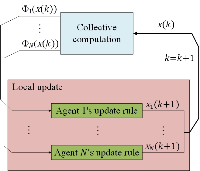
Figure 1: Block diagram of the computation problem (1)

2.3 Attacker model and privacy notions

In this subsection, we identify the attacker model and privacy notions adopted in this paper.

In this paper, we are concerned with semi-honest adversaries, i.e., any adversary $i\in\mathcal{V}\cup\{\rm SO\}$ correctly follows the algorithm but attempts to use its received messages throughout the execution of the algorithm to infer other participants’ private data (Hazay and Lindell (2010), pp-20). Semi-honest adversary model is broadly used in SMC Cramer et al. (2015), Hazay and Lindell (2010) and has been adopted in various applications, e.g., linear programming, dataset process and consensus Dreier and Kerschbaum (2011), Freedman et al. (2004), Huang et al. (2012). Moreover, the system operator is able to eavesdrop all the communication links while we assume that any agent cannot eavesdrop the communication links between other participants. We also assume that the adversaries do not collaborate to infer the information of benign participants. Instead, if multiple adversaries collaborate, they are viewed as a single adversary.

We next introduce the privacy notions adopted in this paper.

$\bullet$ Privacy notion for SMC. We adopt the standard language of view in cryptography to develop the notion.

Consider a set of $M$ parties where each party $i$ holds a set of private data, denoted by $y_{i}\in\mathbb{R}^{d_{i}}$. Let $y=[y_{i}]\in\mathbb{R}^{d}$ with $d=\sum_{i=1}^{M}d_{i}$. Each party $i$ aims to compute a set of functions $h_{i}:\mathbb{R}^{d}\to\mathbb{R}^{r_{i}}$ which depends on the overall $y$. Let $h=[h_{i}]:\mathbb{R}^{d}\to\mathbb{R}^{r}$ with $r=\sum_{i=1}^{M}r_{i}$. Let $\Pi$ be an algorithm that enables the $M$ parties to collectively compute $h$. For each party $i$, its input for $\Pi$ is $y_{i}$. Let $t_{i}$ be the total number of messages received by party $i$ during the execution of $\Pi$ and denote these messages by $v_{1}^{i},\cdots,v_{t_{i}}^{i}$. Given $y$, the view of party $i$ during the execution of $\Pi$, denoted by ${\rm VIEW}_{i}^{\Pi}(y)$, is defined as ${\rm VIEW}_{i}^{\Pi}(y)\buildrel\Delta\over{=}\{y_{i},v_{1}^{i},\cdots,v_{t_{i}}^{i}\}$. To introduce the definition of privacy for SMC, we first need to introduce the definition of computational indistinguishability.

Definition 2.1 (Cramer et al. (2015)).

Let $\mathcal{X}_{[\kappa]}=\{\mathcal{X}_{1},\cdots,\mathcal{X}_{\kappa}\}$ and $\mathcal{Y}_{[\kappa]}=\{\mathcal{Y}_{1},\cdots,\mathcal{Y}_{\kappa}\}$ be two distribution ensembles, where for each $\ell\in\{1,\cdots,\kappa\}$, $\mathcal{X}_{\ell}$ and $\mathcal{Y}_{\ell}$ are random variables with range $R_{\ell}$. We say that $\mathcal{X}_{[\kappa]}$ and $\mathcal{Y}_{[\kappa]}$ are computationally indistinguishable, denoted $X\mathop{\equiv}\limits^{c}Y$, if for every non-uniform probabilistic polynomial-time distinguisher $D$, every positive polynomial $p:\mathbb{N}\to\mathbb{R}_{>0}$, and every sufficiently large $\kappa\in\mathbb{N}$, the following holds:

$$|\Pr[D(\mu)=1]-\Pr[D(\nu)=1]|<{1}/{p(\kappa)}$$

where $\mu$ and $\nu$ are random samples drawn from $\mathcal{X}_{[\kappa]}$ and $\mathcal{Y}_{[\kappa]}$, respectively.  

The following privacy notion for SMC is standard in the literature.

Definition 2.2 (Cramer et al. (2015)).

Let $\Pi$ be an algorithm for computing $h$. We say that $\Pi$ securely computes $h$ if there exists a probabilistic polynomial-time algorithm $S$ such that for each party $i\in\{1,\cdots,M\}$ and every possible $y$, it holds that $S(i,y_{i},h_{i}(y))\mathop{\equiv}\limits^{c}{\rm VIEW}_{i}^{\Pi}(y)$, where $S(\cdot)$ denotes the overall messages that can be seen after the execution of $S$.  

Definition 2.2 states that whatever a party receives during the computing process can be constructed only via its own inputs and the outputs of the functions to compute. In other words, the computing process reveals nothing more than what a party has to learn.

Encryption privacy. In this paper, we use homomorphic encryption to tackle the issue of SMC for the agents. This technique requires some computing entity, which could be semi-honest, to perform function evaluations over encrypted data. In this paper, the system operator is used as the computing entity. Roughly speaking, the agents encrypt their private data and send the encrypted data to the system operator. The system operator evaluates the agents’ functions $\Phi_{i}$’s over the received encrypted data and sends the results to the agents. The agents then decrypt the results to obtain the true values of $\Phi_{i}$’s.

On the one hand, the above homomorphic encryption setting could tackle the SMC issue as the agents only receive aggregate function outputs, but do not receive any form of individual private data. On the other hand, since the system operator could be semi-honest, we need to ensure encryption privacy against the system operator, that is, the system operator cannot infer the private data of the agents from the encrypted data it receives. In the homomorphic encryption literature Yi et al. (2014), Paar and Pelzl (2010), Stallings (2011), two different notions have been widely used to claim or define encryption privacy against the computing entity: (i) plaintexts not efficiently solvable Rivest et al. (1978) and (ii) plaintexts not efficiently distinguishable Goldwasser and Micali (1982). This paper adopts both the two notions, illustrated next.

(i) Plaintexts not efficiently solvable. By this notion, an encryption scheme is secure if the adversaries cannot solve plaintexts via observing ciphertexts by any polynomial-time algorithms. For an encryption scheme that adopts this privacy notion, breaking the scheme (i.e., solving plaintexts) is or is believed to be computationally hard. However, in many cases, it is not proved that the leveraged hard problem itself indeed does not admit a polynomial-time solving algorithm, but rather people have not found one yet. Hence, for this privacy notion, the security level of an encryption scheme is usually not established by a proof, but claimed in a heuristic manner by checking all existing solving algorithms and claiming that none of them is efficient (usually given that the key length is large enough). Well-known encryption schemes that adopt this notion of security and claim their security in this heuristic manner include public key encryption scheme RSA and private key encryption schemes DES (Data Encryption Standard) and AES (Advanced Encryption Standard).

(ii) Plaintexts not efficiently distinguishable. Roughly speaking, an encryption scheme is secure in this sense if the adversaries cannot distinguish between any plaintexts via observing ciphertexts by any polynomial-time algorithms. For the term indistinguishability, informally, it means that given an encryption of a message randomly chosen from any two-element message space determined by the adversary, the adversary cannot identify the message choice with probability significantly better than $0.5$. It is clear that this privacy notion is stronger than the above one, since indistinguishability surely implies unsolvability, but the reverse direction may not be true (it could be hard to find which is the plaintext but easy to tell which is not). A standard definition for this privacy notion is semantic security, defined next.

Definition 2.3 (Cramer et al. (2015)).

Let $E$ be an encryption scheme which outputs ciphertext $E(x)$ on plaintext $x$. An adversary chooses any plaintexts $x,x^{\prime}$ and asks for their ciphertexts from the scheme holder. The scheme holder outputs ciphertexts $E(x)$ and $E(x^{\prime})$ and sends them to the adversary without telling the adversary which ciphertext corresponds to which plaintext. We say that $E$ is semantically secure if for any plaintexts $x,x^{\prime}$ chosen by the adversary in the above setting, it holds that $E(x)\mathop{\equiv}\limits^{c}E(x^{\prime})$ to the adversary.  

Definition 2.3 renders semantically secure encryption schemes provable. Usually, the semantic security of an encryption scheme is established upon an assumption that certain problem is hard to solve, and then the proof of semantic security is performed by reducing the distinguish task to solving the concerned hard problem. Well-known semantically secure encryption schemes include public key encryption schemes Goldwasser-Micali, ElGamal, Paillier and Boneh-Goh-Nissim.

$\bullet$ Privacy notions for IOI. To the best of our knowledge, there is no dominating definition for the question of IOI in cryptography community. In this paper, we adopt the following definition to quantify the uncertainty an adversary has about the private inputs of other parties given the outputs of the functions. The definition is inspired by the notion of observability in control theory and is consistent with the uncertainty based privacy notions in the field of database analysis Marks (1996), Brodsky et al. (2000).

Definition 2.4.

Denote the true valuation of $y_{i}$ by $\bar{y}_{i}$ for each party $i$ and denote $\bar{y}=[\bar{y}_{i}]$. For each party $i$, for each $j\neq i$, denote $\Delta_{j}^{i}(\bar{y})=\{y_{j}\in\mathbb{R}^{d_{j}}:\exists y_{\ell}\in\mathbb{R}^{d_{\ell}}\;{\rm for\;all\;}\ell\neq i,j\;{\rm s.t.}\;h_{i}(\bar{y}_{i},y_{j},[y_{\ell}]_{\ell\neq i,j})=h_{i}(\bar{y})\}$, and denote ${\rm Dist}_{j}^{i}(\bar{y})=\sup_{y_{j},y_{j}^{\prime}\in\Delta_{j}^{i}(\bar{y})}\|y_{j}-y_{j}^{\prime}\|_{2}$. Given $\bar{y}$, for each $j\in\{1,\cdots,M\}$, the amount of uncertainty in $y_{j}$ in the input-output inference of $h$ is defined as $\min_{i\neq j}{\rm Dist}_{j}^{i}(\bar{y})$. We say that the function $h$ resists input-output inference with unbounded uncertainty if the amount of uncertainty in $y_{j}$ is infinite for all $j\in\{1,\cdots,M\}$ and for any $\bar{y}\in\mathbb{R}^{d}$.  

In the subsequent sections, we first study the question of SMC in Sections 3 and 4. After that, we analyze the question of IOI in Section 5.

2.4 Transformation between integers and real numbers

In distributed optimization problems, the variables and coefficients are usually real numbers. However, most existing homomorphic encryption schemes rely on certain modular operations and only work for integers. Therefore, we need a mechanism for transformation between real numbers and integers. Throughout the paper, the accuracy level is set by a parameter $\sigma\in\mathbb{N}$, which means that for any real number, $\sigma$ decimal fraction digits are kept while the remaining decimal fraction digits are dropped. We assume that the value of $\sigma$ is known to the system operator and all the agents. For a real number $r$ with $\sigma$ decimal fraction digits, it is transformed into an integer $z_{r}$ simply by $z_{r}=10^{\sigma}r$. The following function is needed to transform a non-negative integer into a signed real number. Given $\sigma\in\mathbb{N}$ and an odd positive integer $w$, an integer $z\in\mathbb{Z}_{w}$ is transformed into a signed real number with $\sigma$ decimal fraction digits by the following function parameterized by $\sigma$ and $w$:

$$T_{\sigma,w}(z)=\left\{{\begin{array}[]{*{20}{l}}{{z}/{10^{\sigma}},\,{\rm if}\,0\leq z\leq{{(w-1)}}/{2}},\\ {{(z-w)}/{10^{\sigma}},\,{\rm if}\,{{(w+1)}}/{2}\leq z<w}.\end{array}}\right.$$ (4)

The following property holds for the $T$ function (4) and is crucial to guarantee correctness of computations over signed real numbers.

Lemma 2.1.

Given an odd positive integer $w$, for any $r\in\mathbb{R}$ with $\sigma$ decimal fraction digits such that $|10^{\sigma}r|\leq(w-1)/2$, it holds that $T_{\sigma,w}(10^{\sigma}r\mod w)=r$.  

Since $|10^{\sigma}r|\leq(w-1)/2$, it is either $0\leq 10^{\sigma}r\leq(w-1)/2$ or $-(w-1)/2\leq 10^{\sigma}r<0$.

Case I: $0\leq 10^{\sigma}r\leq(w-1)/2$. For this case, we have $10^{\sigma}r\mod w=10^{\sigma}r$. Hence, by (4), we have $T_{\sigma,w}(10^{\sigma}r\mod w)=T_{\sigma,w}(10^{\sigma}r)=(10^{\sigma}r)/10^{\sigma}=r$.

Case II: $-{(w-1)}/{2}\leq 10^{\sigma}r<0$. For this case, we have $10^{\sigma}r\mod w=w+10^{\sigma}r$. It is clear that $(w+1)/2\leq w+10^{\sigma}r<w$. Hence, by (4), we have $T_{\sigma,w}(10^{\sigma}r\mod w)=T_{\sigma,w}(w+10^{\sigma}r)=(w+10^{\sigma}r-w)/10^{\sigma}=r$.

3 Private key secure computation algorithm

In this section, we propose a secure computation algorithm for (1) which is based on a private key fully homomorphic encryption scheme.

3.1 Preliminaries

First, each participant $i\in\mathcal{V}\cup\{\rm SO\}$ constructs a set $\tilde{C}_{\Phi}^{i}$ of coefficients such that $(\tilde{C}_{\Phi}^{1},\cdots,\tilde{C}_{\Phi}^{N},\tilde{C}_{\Phi}^{\rm SO})$ have the following properties: (i) $\tilde{C}_{\Phi}^{\rm SO}=C_{\Phi}^{\rm SO}$; (ii) $\tilde{C}_{\Phi}^{i}\subseteq C_{\Phi}^{i}$ for all $i\in\mathcal{V}$; (iii) the sets $\tilde{C}_{\Phi}^{i}$’s form a partition of $C_{\Phi}$, i.e., $\bigcup_{i\in\mathcal{V}\cup\{\rm SO\}}\tilde{C}_{\Phi}^{i}=C_{\Phi}$ and $\tilde{C}_{\Phi}^{i}\cap\tilde{C}_{\Phi}^{j}=\emptyset$ for any $i,j\in\mathcal{V}\cup\{\rm SO\}$ and $i\neq j$. Such a construction can be realized by a number of ways, e.g., assigning each shared coefficient to the participant with the lowest identity index (assuming that the system operator has identity index 0). Notice that the mutual exclusiveness property above (i.e., $\tilde{C}_{\Phi}^{i}\cap\tilde{C}_{\Phi}^{j}=\emptyset$ for any $i\neq j$) is not possessed by the sets $C_{\Phi}^{i}$’s. This property can guarantee that each coefficient is only encrypted once in the secure computation algorithm (see line 3 of Algorithm 1). This is needed as the privacy of a coefficient could be compromised if it is encrypted multiple times (see the next subsection). For each $i\in\mathcal{V}\cup\{\rm SO\}$, let $m_{i}=|\tilde{C}_{\Phi}^{i}|$ and denote by $c_{i}=[c_{i\ell}]\in\mathbb{R}^{m_{i}}$ the vector of the elements of $\tilde{C}_{\Phi}^{i}$. Let $c=[c_{i}]_{i\in\mathcal{V}\cup\{\rm SO\}}\in\mathbb{R}^{m}$ with $m=\sum_{i\in\mathcal{V}\cup{\rm SO}}m_{i}$ and let $c_{\mathcal{V}}=[c_{i}]_{i\in\mathcal{V}}$.

For each $\Phi_{i\ell}$, we view it as a function of both $x$ and $c$. Denote by $\Phi_{i\ell}^{s}:\mathbb{R}^{n}\times\mathbb{R}^{m}\to\mathbb{R}$ the function with the same structure of $\Phi_{i\ell}$ but takes the coefficients $c$ also as variables and denote by $y=[y_{i}]\in\mathbb{R}^{m}$ the variables corresponding to $c$, where for each $i\in\mathcal{V}\cup{\rm SO}$, $y_{i}\in\mathbb{R}^{m_{i}}$ is the variable corresponding to $c_{i}$. The relation between $\Phi_{i\ell}$ and $\Phi_{i\ell}^{s}$ is then $\Phi_{i\ell}(x)=\Phi_{i\ell}^{s}(x,y)|_{y=c}$.

For each $\Phi_{i\ell}^{s}$, assume that it is written in the canonical form, i.e., sum of monomials, and denote by $\kappa_{i\ell}$ the number of monomials of $\Phi_{i\ell}^{s}$ and $Q_{i\ell}^{v}:\mathbb{R}^{n}\times\mathbb{R}^{m}\to\mathbb{R}$ the $v$-th monomial of $\Phi_{i\ell}^{s}$. Then, $\Phi_{i\ell}^{s}$ can be written as $\Phi_{i\ell}^{s}(x,y)=\sum_{v=1}^{\kappa_{i\ell}}Q_{i\ell}^{v}(x,y)$.

3.2 An illustrative example

We first use an illustrative example to demonstrate the major challenges in the algorithm design. Consider the scenario of two agents and a system operator. Each agent $i\in\{1,2\}$ has a scalar state $x_{i}\in\mathbb{R}$. The joint functions of the two agents are $\Phi_{1}(x_{1},x_{2})=c_{1}x_{1}^{2}+c_{2}x_{1}x_{2}+c_{3}x_{1}$ and $\Phi_{2}(x_{1},x_{2})=c_{1}c_{2}x_{2}$, respectively, where $c_{1},c_{2},c_{3}\in\mathbb{R}$ are the private coefficients of agent 1 and $c_{2}\in\mathbb{R}$ is the private coefficient of agent 2.

We next illustrate why existing homomorphic encryption schemes cannot be directly used to solve the above problem and clarify how the challenges are addressed.

(i) Transformation between real numbers and integers. Existing homomorphic encryption schemes only work for binary numbers or non-negative integers and hence cannot be directly applied to the above problem, where the coefficients $(c_{1},c_{2},c_{3})$ and the states $(x_{1},x_{2})$ are all signed real numbers. We overcome this challenge by proposing the transformation mechanism (4) between integers and real numbers. Roughly speaking, before encrypting a real data item, say $c_{1}$, with $\sigma$ decimal fraction digits, one first transforms it into an integer $10^{\sigma}c_{1}$. One can then apply a specific homomorphic encryption scheme, which will be discussed in the next paragraphs, to perform encryption, computation and decryption operations over the transformed integers. After that, the decrypted integer result is transformed back to a signed real number by the transformation mechanism (4).

(ii) Sum operation over transformed integers. As mentioned in the last paragraph, before encrypting a real data item, say $c_{1}$, with $\sigma$ decimal fraction digits, one first transforms it into an integer $10^{\sigma}c_{1}$. This essentially scales the magnitude of $c_{1}$ by $10^{\sigma}$ times. Now let agent 1 form the monomials using the transformed integers $(10^{\sigma}x_{1},10^{\sigma}c_{1},10^{\sigma}c_{2},10^{\sigma}c_{3})$. Since $Q_{1}^{1}$ and $Q_{1}^{2}$ have degree 3, they are scaled by $10^{3\sigma}$ times, i.e., $Q_{1}^{1}(10^{\sigma}x,10^{\sigma}c)=10^{\sigma}c_{1}\cdot(10^{\sigma}x_{1})^{2}=10^{3\sigma}c_{1}x_{1}^{2}$ and $Q_{1}^{2}(10^{\sigma}x,10^{\sigma}c)=10^{\sigma}c_{2}\cdot 10^{\sigma}x_{1}\cdot 10^{\sigma}x_{2}=10^{3\sigma}c_{2}x_{1}x_{2}$. Since $Q_{1}^{3}$ has degree 2, it is scaled by $10^{2\sigma}$ times, i.e., $Q_{1}^{3}(10^{\sigma}x,10^{\sigma}c)=10^{\sigma}c_{3}\cdot 10^{\sigma}x_{1}=10^{2\sigma}c_{3}x_{1}$. Hence, with the transformed integers, the monomials $Q_{1}^{1}$, $Q_{1}^{2}$ and $Q_{1}^{3}$ are scaled by different times and thus the sum operation between them cannot be directly applied. We overcome this challenge by multiplying each monomial $Q_{i}^{\ell}$ formed with the transformed integers by a scaling term $10^{({\rm deg}(\Phi_{i}^{s})-{\rm deg}(Q_{i}^{\ell}))\sigma}$. In particular, the scaled $Q_{1}^{1}$, $Q_{1}^{2}$ and $Q_{1}^{3}$ become $\hat{Q}_{1}^{1}=10^{(3-3)\sigma}10^{3\sigma}c_{1}x_{1}^{2}=10^{3\sigma}c_{1}x_{1}^{2}$, $\hat{Q}_{1}^{2}=10^{(3-3)\sigma}10^{3\sigma}c_{2}x_{1}x_{2}=10^{3\sigma}c_{2}x_{1}x_{2}$ and $\hat{Q}_{1}^{3}=10^{(3-2)\sigma}10^{2\sigma}c_{3}x_{1}=10^{3\sigma}c_{3}x_{1}$, respectively. Notice that the scaled monomials $(\hat{Q}_{1}^{1},\hat{Q}_{1}^{2},\hat{Q}_{1}^{3})$ remain integers and simultaneously they are all scaled by $10^{3\sigma}$ times and hence the sum operation between them can be applied. The above method is generalized in line 6 of Algorithm 1.

(iii) Encryption of coefficients held by multiple agents. In the above example, $c_{2}$ is a private coefficient of both agent 1 and agent 2. A question is whether the security of $c_{2}$ could be compromised when it is encrypted by both agent 1 and agent 2. To answer this question, we first need to choose a homomorphic encryption scheme. The above example includes both addition and multiplication operations. Hence, we need to use a fully homomorphic encryption scheme. To the best of our knowledge, there does not exist a fully homomorphic encryption scheme for integers which is both efficiently implementable and semantically secure. Please refer to Section 9.1 for a summary of existing homomorphic encryption schemes. In this section, we choose the SingleMod encryption Phatak et al. (2014) as our designing prototype, because it is an efficiently implementable (private key) fully homomorphic encryption scheme (for integers). On the other hand, the SingleMod encryption is not semantically secure. Instead, its security level adopts the standard notion of Plaintexts not efficiently solvable (see Section 2.3). As mentioned in Section 2.3, many widely used encryption schemes adopt this notion of security, e.g., RSA, DES and AES. Since the SingleMod encryption is not semantically secure, the security of $c_{2}$ could be compromised if it is encrypted by both agent 1 and agent 2. For the SingleMod encryption, agent 1 and agent 2 agree on a large positive integer key $w$ and keep it secret from the system operator. To encrypt a non-negative integer $t<w$, one chooses an arbitrary positive integer $u_{t}$ and encrypts $t$ by $\hat{t}=u_{t}w+t$. Now assume that agent 1 and agent 2 encrypt $10^{\sigma}c_{2}$ (recall that $10^{\sigma}c_{2}$ is an integer) by $\hat{y}_{2}^{\prime}=u_{y_{2}}^{\prime}w+10^{\sigma}c_{2}$ and $\hat{y}_{2}^{\prime\prime}=u_{y_{2}}^{\prime\prime}w+10^{\sigma}c_{2}$, respectively, where $u_{y_{2}}^{\prime}$ (resp. $u_{y_{2}}^{\prime\prime}$) is an arbitrary positive integer only known to agent 1 (resp. 2). By knowing $\hat{y}_{2}^{\prime}$ and $\hat{y}_{2}^{\prime\prime}$, the system operator can compute $\hat{y}_{2}^{\prime}-\hat{y}_{2}^{\prime\prime}=(u_{y_{2}}^{\prime}-u_{y_{2}}^{\prime\prime})w$. Notice that $u_{y_{2}}^{\prime}$, $u_{y_{2}}^{\prime\prime}$, $\hat{y}_{2}^{\prime}$, $\hat{y}_{2}^{\prime\prime}$ and $w$ are all integers. The system operator can then tell that $w$ must be a factor of $\hat{y}_{2}^{\prime}-\hat{y}_{2}^{\prime\prime}$. In the worst case where $u_{y_{2}}^{\prime}-u_{y_{2}}^{\prime\prime}$ and $w$ are both prime numbers, there are only two possible values for $w$. Assume $|10^{\sigma}c_{2}|\leq(w-1)/2$ (which is usually true as $w$ needs to be chosen very large for the concern of security). By Lemma 2.1, for each possible $w$, since the system operator knows the values of $\sigma$ and $\hat{y}_{2}^{\prime}$, it can obtain a unique value of $c_{2}$ by computing $c_{2}=T_{\sigma,w}(10^{\sigma}c_{2}\mod w)=T_{\sigma,w}(\hat{y}_{2}^{\prime}\mod w)$. By Definition 2.3, this indicates that the SingleMod encryption is not semantically secure. By the above procedure, the system operator can obtain a good estimate of $c_{2}$. We overcome this challenge by constructing a partition of the coefficient set $C_{\Phi}$ as illustrated in Section 3.1 so that it is guaranteed that each private coefficient is only encrypted once. For this example, the partition could be either $\tilde{C}_{\Phi}^{1}=\{c_{1},c_{2},c_{3}\}$ and $\tilde{C}_{\Phi}^{2}=\emptyset$ in which agent 1 encrypts $c_{2}$, or $\tilde{C}_{\Phi}^{1}=\{c_{1},c_{3}\}$ and $\tilde{C}_{\Phi}^{2}=\{c_{2}\}$ in which agent 2 encrypts $c_{2}$.

(iv) Causal attacks by the system operator. Assume that the system operator can use the data received up to time instant $k$ to infer $x(k)$. Again, due to that the SingleMod encryption is not semantically secure, the system operator could succeed if it fully knows the update rule of $x(k)$. We now assume that $c_{1}$ and $c_{2}$ are private coefficients of the system operator, $X_{2}=\mathbb{R}$, $\gamma(1)=1$, and these are known to the system operator. By (1), the system operator can derive $x_{2}(2)=(1-c_{1}c_{2})x_{2}(1)$. Now agent 2 encrypts $x_{2}(1)$ and $x_{2}(2)$ by $\hat{x}_{2}(1)=u_{x_{2}}(1)w+10^{\sigma}x_{2}(1)$ and $\hat{x}_{2}(2)=u_{x_{2}}(2)w+10^{\sigma}x_{2}(2)$, respectively. By knowing $x_{2}(2)=(1-c_{1}c_{2})x_{2}(1)$, the system operator can obtain $\hat{x}_{2}(2)-(1-c_{1}c_{2})\hat{x}_{2}(1)=(u_{x_{2}}(2)-(1-c_{1}c_{2})u_{x_{2}}(1))w$ and know that $w$ is a factor of $\hat{x}_{2}(2)-(1-c_{1}c_{2})\hat{x}_{2}(1)$. Similar to the discussion in (iii), by knowing $\sigma$, $\hat{x}_{2}(1)$ and $\hat{x}_{2}(2)$, the system operator can then obtain a good estimate of $x_{2}(1)$ and $x_{2}(2)$. We overcome this challenge by assuming that the system operator can only launch temporarily independent attacks. Please refer to Assumption 3.2. This assumption has been widely used in database privacy. Please refer to Remark 3.2 for the detailed discussion of this assumption.

3.3 Algorithm design and analysis

The private key secure computation algorithm for (1) is presented by Algorithm 1. This algorithm is based on the SingleMod encryption Dijk et al. (2010), Phatak et al. (2014). As mentioned in item (iii) of Section 3.2, the SingleMod encryption is an efficiently implementable private key fully homomorphic encryption scheme for integers. The encryption privacy of our encryption scheme shares the same privacy notion with that of the SingleMod encryption, i.e., Plaintexts not efficiently solvable (see Section 2.3). In particular, for our case, breaking the scheme is as hard as the approximate greatest common divisor (GCD) problem , which is widely believed to be NP-hard Dijk et al. (2010), Phatak et al. (2014).

Algorithm 1 Private key secure computation algorithm

1. Initialization: Each agent $i$ chooses any $x_{i}(0)\in X_{i}$;

2. Key agreement: All agents agree on a large odd positive integer $w$ and keep $w$ secret from SO;

3. Coefficient encryption: Each agent $i$ chooses any $u_{y_{i}}\in\mathbb{Z}_{>0}^{m_{i}}$ and sends to SO $\hat{y}_{i}$ computed as $\hat{y}_{i}=u_{y_{i}}w+10^{\sigma}c_{i}$; SO forms $\hat{y}=[\hat{y}_{j}]_{j\in\mathcal{V}\cup\{\rm SO\}}$ with $\hat{y}_{\rm SO}=10^{\sigma}c_{\rm SO}$;

4. while $k\geq 0$

5.  State encryption: Each agent $i$ chooses any $u_{x_{i}}(k)\in\mathbb{Z}_{>0}^{n_{i}}$ and sends to SO $\hat{x}_{i}(k)$ computed as $\hat{x}_{i}(k)=u_{x_{i}}(k)w+10^{\sigma}x_{i}(k)$; SO forms $\hat{x}(k)=[\hat{x}_{j}(k)]_{j\in\mathcal{V}}$;

6.  Computation over ciphertexts: For each $i\in\mathcal{V}$, for each $\ell=1,\cdots,n_{i}$, SO sends $\bar{\Phi}_{i\ell}^{s}(k)$ to agent $i$ computed as:

$$\bar{\Phi}_{i\ell}^{s}(k)= \sum\nolimits_{v=1}^{\kappa_{i\ell}}[10^{({\rm deg}(\Phi_{i\ell}^{s})-{\rm deg}(Q_{i\ell}^{v}))\sigma}Q_{i\ell}^{v}(\hat{x}(k),\hat{y})];$$

7.  Decryption: For each $i\in\mathcal{V}$, for each $\ell=1,\cdots,n_{i}$, agent $i$ computes $\hat{\Phi}_{i\ell}^{s}(k)=T_{{\rm deg}(\Phi_{i\ell}^{s})\sigma,w}(\bar{\Phi}_{i\ell}^{s}(k)\mod w)$;

8.  Local update: Each agent $i$ forms $\hat{\Phi}_{i}^{s}(k)=[\hat{\Phi}_{i\ell}^{s}(k)]$ and computes $x_{i}(k+1)=\mathbb{P}_{X_{i}}[x_{i}(k)-\gamma(k)\hat{\Phi}_{i}^{s}(k)]$;

9.   Set $k\leftarrow k+1$;

10. end while

The algorithm is informally stated next. At line 2, all the agents agree on a key $w$ and keep the value of $w$ unknown to the system operator. One case where such key agreement is possible is that the sub-communication graph between the agents is connected and all its communication links are secure .

For the sake of security, $w$ is chosen as a very large number, e.g., in the magnitude of $2^{2000}$ Giry (2017). On the other hand, to guarantee the correctness of decryption (line 7) which is a modulo operation over $w$, the value of $w$ cannot be too small. Roughly speaking, the value of $w$ must be larger than all possible plaintexts of computing results. This is captured by the following assumption.

Assumption 3.1.

The key $w$ is chosen large enough such that, for any step $k$, it holds that $w\geq 1+2\max_{i,\ell}10^{{\rm deg}(\Phi_{i\ell}^{s})\sigma}|\Phi_{i\ell}(x(k))|$.  

Remark 3.1.

A sufficient condition for Assumption 3.1 is that $x$ lives in a compact set whose bound is known to the agents a priori. In the cases where this sufficient condition does not hold, since $w$ needs to be chosen very large for the sake of security, Assumption 3.1 is usually automatically satisfied. In Section 6, we provide concrete examples for which this is true.  

At line 3, each agent $i$ encrypts its coefficient $c_{i}$ via the SingleMod encryption using the private key $w$ and a random integer vector $u_{y_{i}}$. Recall that any involved real number has (at most) $\sigma$ decimal fraction digits. Hence, $10^{\sigma}c_{i}$ is an integer vector. Since $c_{i}$ is fixed throughout the computing process, it only has to be encrypted once.

At line 5, each agent $i$ encrypts its current state $x_{i}(k)$ via the SingleMod encryption using the key $w$ and a random integer vector $u_{x_{i}}(k)$. Notice that at each iteration, the encryption of $x_{i}(k)$ adopts a new randomness $u_{x_{i}}(k)$.

Line 6 is the computation step at which the system operator computes each function $\Phi_{i\ell}^{s}$ by the encrypted data $(\hat{x}(k),\hat{y})$. For each $v=1,\cdots,\kappa_{i\ell}$, $Q_{i\ell}^{v}(\hat{x}(k),\hat{y})$ is multiplied by $10^{({\rm deg}(\Phi_{i\ell}^{s})-{\rm deg}(Q_{i\ell}^{v}))\sigma}$ in order to have each monomial scaled by the same times so that the sum operation can be performed. In particular, without the $u_{x_{i}}(k)w$ (resp. $u_{y_{i}}w$) part (which is eliminated by modulo operation in the decryption step), each $x_{i}(k)$ (resp. $c_{i}$) is scaled by $10^{\sigma}$ times in the integer transformation operation at line 5 (resp. 3). Each $Q_{i\ell}^{v}(\hat{x}(k),\hat{y})$ is then scaled by $10^{{\rm deg}(Q_{i\ell}^{v})\sigma}$ times and $10^{({\rm deg}(\Phi_{i\ell}^{s})-{\rm deg}(Q_{i\ell}^{v}))\sigma}Q_{i\ell}^{v}(\hat{x}(k),\hat{y})$ is scaled by $10^{{\rm deg}(\Phi_{i\ell}^{s})\sigma}$ times. Thus, all the monomials of $\Phi_{i\ell}^{s}$ are scaled by the same times and can be summed up.

Line 7 is the decryption step. Each agent $i$ first performs modulo operation over the encrypted function value $\bar{\Phi}_{i\ell}^{s}(k)$ by the private key $w$ which eliminates all terms having $w$ as a factor. Then, agent $i$ transforms the resulted integer back into a signed real number by the $T$ function defined by (4).

Line 8 is the local update step. Each agent $i$ updates $x_{i}(k)$ by (1) by using $\hat{\Phi}_{i}^{s}(k)$ as $\Phi_{i}(x(k))$.

To help with understanding, we provide a numerical example in Section 9.3.1 to go through the steps of Algorithm 1.

Assumption 3.2.

The system operator can only perform temporarily independent attacks, i.e., at each step $k$, it uses the data received at step $k$ to infer $x(k)$, but does not use past data to collectively infer the sequence $x(0),\cdots,x(k)$.  

Remark 3.2.

One case where Assumption 3.2 holds is that the system operator is not fully aware of the update rule of $x(k)$ and views the sequence $\{x(k)\}$ as a temporally independent time series Shi et al. (2011). For example, the system operator could be an untrustworthy third party who does not know the underlying update rule (1) or even does not know what problem the agents aim to solve Roy et al. (2012). In this scenario, the system operator only receives a sequence of (encrypted) aggregate results from an unknown system. This scenario has been widely considered in database privacy and many works in the field are based on the temporal independence assumption. For example, the work Bhaskar et al. (2011), which studied noiseless database privacy, explicitly made the assumption that the entries in the database are uncorrelated and justified the assumption by that, without knowing a system, observing aggregate information released from the system may provide little knowledge on the correlation of the entries. Moreover, as pointed out by Dwork et al. (2005) and Chapter 14 of Zhu et al. (2017), most existing differential privacy works assume that the dataset consists of independent records, despite the fact that records in real world applications are often correlated.  

Theorem 3.1.

Suppose that Assumptions 2.1, 2.2, 3.1 and 3.2 hold. By Algorithm 1, the following claims hold:

1) Correctness: $\hat{\Phi}_{i}^{s}(k)=\Phi_{i}(x(k))$ for any $k$ and $i\in\mathcal{V}$.

2) Security: Between the agents, Algorithm 1 securely computes the sequence of $\{\Phi_{1}(x(k)),\cdots,\Phi_{N}(x(k))\}$; for the system operator, at each step $k$, Algorithm 1 is as hard as the approximate GCD problem for the system operator to solve $x(k)$ and $c_{\mathcal{V}}$.  

The proof of Theorem 3.1 is given in Section 7.1. In the proof, the privacy notion of plaintexts not efficiently solvable (Section 2.3) and Definition 2.2 are used. In particular, the correctness is derived by exploring the homomorphic property of the proposed private key encryption scheme and the property of the proposed real-integer transformation scheme (Lemma 2.1). The secure computation result between the agents is obtained by using the simulation paradigm which is a standard technique for proving SMC Cramer et al. (2015), Lindell and Pinkas (2009). The security level against the system operator is based on the fact that solving $x(k)$ and $c_{\mathcal{V}}$ is exactly the approximate GCD problem.

Remark 3.3.

The encryption scheme of Algorithm 1 leverages the SingleMod encryption. As pointed out in Phatak et al. (2014), the SingleMod encryption is not semantically secure. Instead, the encryption privacy of the SingleMod encryption is claimed in the sense of Plaintexts not efficiently solvable. On the one hand, this privacy notion is weaker than semantic security Yi et al. (2014). On the other hand, the weaker security level renders that Algorithm 1 is fully homomorphic and efficiently implementable (see Section 6.1 for efficiency). As mentioned in Section 2.3, this sense of privacy claim has been adopted in many widely used encryption schemes, e.g., RSA, DES and AES. In the next section, we assume that the joint functions are affine and provide a partially homomorphic encryption scheme which possesses semantic security.  

4 Public key secure computation algorithm

Algorithm 1 proposed in the last section has several limitations: key distribution problem exists as the agents have to agree on a private key; its security level against the system operator is not semantic security, and as a consequence, it can only resist temporarily independent attacks against the system operator. In this section, we consider the special case where $\Phi_{i\ell}$’s are affine functions and propose a public key secure computation algorithm to address these limitations. To be more specific, the class of computation problems considered in this section is specified by the following assumption.

Assumption 4.1.

For each $i\in\mathcal{V}$ and each $\ell\in\{1,\cdots,n_{i}\}$, the function $\Phi_{i\ell}$ is affine in $x$ and the coefficients of $\Phi_{i\ell}$ are all known to the system operator.  

Remark 4.1.

Assumption 4.1 indicates that each agent $i$’s coefficients are known to the system operator but may not be known to other agents.

The reason that Assumption 4.1 is needed for this section is that the Paillier encryption scheme adopted in this section is only additively homomorphic but not multiplicatively homomorphic. Thus, we need the desired functions $\Phi_{i\ell}$’s to be affine in $x$. Moreover, if the function to be computed is a weighted sum of $x$, then the weights (transformed into integers) must be known by the entity who performs the computation (the system operator in our algorithm) so that the multiplication of a weight and a variable can be carried out by summing up the variable with itself for certain times (see (3-ii) of Theorem 9.1). A similar treatment as Assumption 4.1 was adopted in Freris and Patrinos (2016) in the context of encrypted average consensus.

To the best of our knowledge, all computationally efficient public key homomorphic encryption schemes are partially homomorphic, e.g., the RSA scheme Rivest et al. (1978) and the ElGamal scheme ElGamal (1985) are multiplicatively homomorphic, and the Goldwasser–Micali scheme Goldwasser and Micali (1982) and the Paillier scheme Paillier (1999) are additively homomorphic. The first fully public key homomorphic encryption scheme was developed by Gentry in his seminal work Gentry (2009). However, due to that the Gentry fully homomorphic encryption scheme uses lattice and bootstrapping, its implementation is rather complicated and time-consuming, which significantly limits its applications in practice.

As mentioned in Section 2.1, $\Phi_{i}$ is the first-order gradient of certain functions with respect to $x_{i}$. A sufficient and necessary condition for the affinity assumption is that the associated component functions are affine or quadratic in $x_{i}$. Hence, problem (1) satisfying Assumption 4.1 covers a large class of problems, e.g., linear and quadratic programs Bertsekas and Tsitsiklis (1997), quadratic convex games Zhu and Frazzoli (2016) and affine variational inequalities Facchinei and Pang (2003).  

By Assumption 4.1, each function $\Phi_{i\ell}$ is a weighted sum of $x$ for which the weights are known to the system operator. For convenience of notation, we write each $\Phi_{i\ell}$ as:

$$\Phi_{i\ell}(x)=\sum\nolimits_{j=1}^{N}\sum\nolimits_{v=1}^{n_{j}}A_{i\ell}^{jv}x_{jv}+B_{i\ell}$$ (5)

where $A_{i\ell}^{jv}\in\mathbb{R}$ and $B_{i\ell}\in\mathbb{R}$ are coefficients known to the system operator. For each $j\in\mathcal{V}$, let $A_{i\ell}^{j}=[A_{i\ell}^{j1},\cdots,A_{i\ell}^{jn_{j}}]$ and $A_{i}^{j}=[A_{i\ell}^{j}]_{\ell\in\{1,\cdots,n_{i}\}}$. For each $i\in\mathcal{V}$, let $A_{i\ell}=[A_{i\ell}^{1},\cdots,A_{i\ell}^{N}]$ for each $\ell=1,\cdots,n_{i}$, $A_{i}=[A_{i}^{1},\cdots,A_{i}^{N}]$ and $B_{i}=[B_{i1},\cdots,B_{in_{i}}]^{T}$. Let $A=[A_{i}]_{i\in\mathcal{V}}$ and $B=[B_{i}]_{i\in\mathcal{V}}$. By these notations, we have $\Phi_{i\ell}(x)=\sum\nolimits_{j=1}^{N}A_{i\ell}^{j}x_{j}+B_{i\ell}=A_{i\ell}x+B_{i\ell}$ and $\Phi_{i}(x)=\sum\nolimits_{j=1}^{N}A_{i}^{j}x_{j}+B_{i}=A_{i}x+B_{i}$.

In this section, we use the Paillier encryption scheme as our design prototype. This is because the Paillier encryption scheme is an efficiently implementable (public key) additively homomorphic encryption scheme (for integers). Again, we use the proposed transformation mechanism (4) to overcome the challenge of signed real numbers. The other challenges illustrated in Section 3.2 do not exist for this case. Since the monomials $A_{i\ell}^{jv}x_{jv}$’s have the same degree, challenge (ii) in Section 3.2 does not exist. Since we assume that the coefficients $A_{i\ell}^{jv}$’s and $B_{i\ell}$’s are all known to the system operator, the agents do not have to encrypt any coefficient and hence challenge (iii) in Section 3.2 does not exist. Since the Paillier encryption scheme is semantically secure, challenge (iv) in Section 3.2 does not exist. Informally speaking, this is because even if the system operator fully knows the relation between some $x_{i}(k)$ and $x_{i}(k+1)$, by Definition 2.3, the encryptions of $x_{i}(k)$ and $x_{i}(k+1)$ provide zero knowledge to the system operator.

4.1 Algorithm design and analysis

The algorithm developed in this section is based on a public key partially homomorphic encryption scheme, namely, the Paillier encryption scheme Paillier (1999). The preliminaries for the Paillier encryption scheme are provided in Section 9.2.

Algorithm 2 Public key secure computation algorithm

1. Initialization: Each agent $i$ chooses any $x_{i}(0)\in X_{i}$;

2. Key generation: Each agent $i$ generates Paillier keys $(\alpha_{i},\beta_{i},\nu_{i},\pi_{i})$, publicizes $(\alpha_{i},\beta_{i})$ while keeps $(\nu_{i},\pi_{i})$ private;

3. while $k\geq 0$

4.  State encryption: For each $i\in\mathcal{V}$ and $\ell\in\{1,\cdots,n_{i}\}$, for each $j\in\mathcal{V}$, agent $i$ selects any $r_{i\ell}^{j}(k)\in\mathbb{Z}_{\alpha_{j}}^{*}$ and sends to SO $\hat{x}_{i\ell}^{j}(k)=\beta_{j}^{10^{\sigma}x_{i\ell}(k)\mod\alpha_{j}}\cdot r_{i\ell}^{j}(k)^{\alpha_{j}}\mod\alpha_{j}^{2}$;

5.  Computation over ciphertexts: For each $i\in\mathcal{V}$ and $\ell\in\{1,\cdots,n_{i}\}$, SO sends $\bar{\Phi}_{i\ell}^{s}(k)$ to agent $i$ computed as:

$$\bar{\Phi}_{i\ell}^{s}(k)= (\beta_{i}^{10^{2\sigma}B_{i\ell}\!\!\!\!\!\mod\!\alpha_{i}}\prod\limits_{j=1}^{N}\prod\limits_{v=1}^{n_{j}}\hat{x}_{jv}^{i}(k)^{10^{\sigma}A_{i\ell}^{jv}\!\!\!\!\!\mod\!\alpha_{i}})\!\!\!\!\!\mod\!\alpha_{i}^{2};$$

6.  Decryption: For each $i\in\mathcal{V}$ and $\ell\in\{1,\cdots,n_{i}\}$, agent $i$ computes $\hat{\Phi}_{i\ell}^{s}(k)=T_{2\sigma,\alpha_{i}}(\frac{(\bar{\Phi}_{i\ell}^{s}(k)^{\nu_{i}}\mod\alpha_{i}^{2})-1}{\alpha_{i}}\cdot\pi_{i}\mod\alpha_{i})$;

7.  Local update: Each agent $i$ forms $\hat{\Phi}_{i}^{s}(k)=[\hat{\Phi}_{i\ell}^{s}(k)]$ and computes $x_{i}(k+1)=\mathbb{P}_{X_{i}}[x_{i}(k)-\gamma(k)\hat{\Phi}_{i}^{s}(k)]$;

8.   Set $k\leftarrow k+1$;

9. end while

The public key secure computation algorithm for (1) satisfying Assumption 4.1 is presented by Algorithm 2.

At line 2, each agent $i$ generates its Paillier keys $(\alpha_{i},\beta_{i},\nu_{i},\pi_{i})$, where $(\alpha_{i},\beta_{i})$ are public keys known to all participants while $(\nu_{i},\pi_{i})$ are private keys only known to agent $i$. For the sake of security, the keys are chosen very large, e.g., in the magnitude of $2^{2000}$ Giry (2017). To guarantee decryption correctness, we need the following Assumption 4.2. Remark 3.1 applies to this assumption.

Assumption 4.2.

For each agent $i$, its public key $\alpha_{i}$ is chosen large enough such that, for any step $k$, it holds that $\alpha_{i}\geq 1+2\times 10^{2\sigma}\|A_{i}x(k)+B_{i}\|_{\max}$.  

Line 4 is the encryption step. Each agent $i$ encrypts $x_{i}(k)$ by the Paillier encryption operation $N$ times such that the $j$-th encryption uses agent $j$’s public keys $(\alpha_{j},\beta_{j})$ and the corresponding encrypted data $\hat{x}_{i}^{j}(k)$ is used for the computation of agent $j$’s desired functions $\Phi_{j}(x(k))$. By receiving $\hat{x}_{i\ell}^{j}(k)$ and only knowing agent $j$’s public keys $(\alpha_{j},\beta_{j})$, under the decisional composite residuosity assumption (DCRA) , it is computationally intractable for the system operator to infer $x_{i\ell}(k)$.

Line 5 is the computation step. The computation performed by the system operator is based on the additively homomorphic property of the Paillier encryption scheme, i.e., roughly speaking, the multiplication of ciphertexts provides the encryption of the sum of the corresponding plaintexts (see Section 9.2).

Line 6 is the decryption step. Agent $i$ decrypts each $\bar{\Phi}_{i\ell}^{s}(k)$ by the Paillier decryption operation and transforms the decrypted non-negative integer into a signed real number by the $T$ function defined by (4).

Line 7 is the local update step. Each agent $i$ updates $x_{i}(k)$ by (1) by using $\hat{\Phi}_{i}^{s}(k)$ as $\Phi_{i}(x(k))$.

To help with understanding, we provide a numerical example in Section 9.3.2 to go through the steps of Algorithm 2.

Theorem 4.1.

Suppose that Assumptions 2.1, 4.1, 4.2 and the standard cryptographic assumption DCRA hold. By Algorithm 2, the following claims hold:

1) Correctness: $\hat{\Phi}_{i}^{s}(k)=\Phi_{i}(x(k))$ for any $k$ and $i\in\mathcal{V}$.

2) Security: Algorithm 2 securely computes the sequence of $\{\Phi_{1}(x(k)),\cdots,\Phi_{N}(x(k))\}$ between the agents and is semantically secure against the system operator.  

The proof of Theorem 4.1 is given in Section 7.2. In the proof, Definitions 2.3 and 2.2 are used. In particular, the correctness is derived by the homomorphic properties of the Paillier encryption scheme (part (3) of Theorem 9.1) and the property of the proposed real-integer transformation scheme (Lemma 2.1). The secure computation result between agents is obtained by using the simulation paradigm. The semantic security against the system operator follows the semantic security of the Paillier encryption scheme (combination of part (2) of Theorem 9.1 and Theorem 5.2.10 of Goldreich (2004)).

5 Privacy analysis on input-output inference

In the last two sections, we provide two algorithms to achieve SMC. However, as pointed out in Section 2.2, it is possible that the adversary could infer the private inputs of the securely computed functions purely from its own inputs and the function outputs. In this section, we study the second problem raised in Section 2.2, that is, whether the private inputs of a function can be uniquely determined from its outputs.

Recall that $\Phi_{i}^{s}$ denotes the function with the same structure of $\Phi_{i}$ but takes the coefficients $c$ also as variables (see Section 3.1). Denote by $(\{\bar{x}(k)\},\bar{X},\bar{c})$ the true values of $(\{x(k)\},X,c)$. For each $i\in\mathcal{V}$, agent $i$ aims to find feasible $(\{\hat{x}_{-i}(k)\},\hat{X}_{-i},\hat{c}_{-i})$ that satisfy its observations: $\Phi_{i}^{s}(\bar{x}_{i}(k),\hat{x}_{-i}(k),\bar{c}_{i},\hat{c}_{-i})=\Phi_{i}(\bar{x}(k))$ for all $k\in\mathbb{N}$, and $\hat{x}_{j}(k+1)=\mathbb{P}_{\hat{X}_{j}}[\hat{x}_{j}(k)-\gamma(k)\Phi_{j}^{s}(\bar{x}_{i}(k),\hat{x}_{-i}(k),\bar{c}_{i},\hat{c}_{-i})]$ for all $j\in\mathcal{V}\backslash\{i\}$ and all $k\in\mathbb{N}$. By Definition 2.4, the sequence of functions $\{\Phi(x(k))\}$ resists input-output inference with unbounded uncertainty if, for any agent $i\in\mathcal{V}$, each element of the feasible set $\{\{\hat{x}_{-i}(k)\},\hat{X}_{-i},\hat{c}_{-i}\}$ has unbounded uncertainty.

In this section, we study the scenario where $\Phi_{i\ell}$’s are a class of quadratic functions specified by the following assumption.

Assumption 5.1.

For each $i\in\mathcal{V}$ and each $\ell=1,\cdots,n_{i}$, $\Phi_{i\ell}(x)=x^{T}H_{i\ell}x+A_{i\ell}x+B_{i\ell}$, where $H_{i\ell}\in\mathbb{R}^{n\times n}$ and $A_{i\ell}\in\mathbb{R}^{1\times n}$ are public constant matrix and vector, respectively, that are known to all the agents, while $B_{i\ell}\in\mathbb{R}$ is a private constant scalar only known to a subset of agents.  

5.1 An illustrative example

We first use an illustrative example to show the issue of input-output inference. Consider the case of three agents in which agent 1 is adversary and agent 2 and agent 3 are benign. Each agent $i\in\{1,2,3\}$ has a scalar state $x_{i}\in\mathbb{R}$. The joint functions of the three agents are $\Phi_{1}(x_{1},x_{2},x_{3})=-x_{2}-x_{3}$, $\Phi_{2}(x_{1},x_{2},x_{3})=-2x_{3}$ and $\Phi_{3}(x_{1},x_{2},x_{3})=-x_{1}$, respectively. For ease of presentation, assume $X_{i}=\mathbb{R}$ for all $i\in\{1,2,3\}$ and $\gamma(k)=1$ for all $k\in\mathbb{N}$, and these are known to all the three agents. By (1), we then have $x_{1}(k+1)=x_{1}(k)+x_{2}(k)+x_{3}(k)$, $x_{2}(k+1)=x_{2}(k)+2x_{3}(k)$ and $x_{3}(k+1)=x_{1}(k)+x_{3}(k)$. We next show that by knowing $x_{1}(k)$, $x_{1}(k+1)$ and $x_{1}(k+2)$, agent 1 can uniquely determine $x_{2}(k)$ and $x_{3}(k)$. Agent 1 knows $x_{1}(k+1)=x_{1}(k)+x_{2}(k)+x_{3}(k)$ and $x_{1}(k+2)=x_{1}(k+1)+x_{2}(k+1)+x_{3}(k+1)$. By plugging the relations $x_{2}(k+1)=x_{2}(k)+2x_{3}(k)$ and $x_{3}(k+1)=x_{1}(k)+x_{3}(k)$ into $x_{1}(k+2)=x_{1}(k+1)+x_{2}(k+1)+x_{3}(k+1)$, agent 1 derives $x_{2}(k)+3x_{3}(k)=x_{1}(k+2)-x_{1}(k+1)-x_{1}(k)$. Together with the equation $x_{2}(k)+x_{3}(k)=x_{1}(k+1)-x_{1}(k)$, agent 1 can uniquely derive $x_{2}(k)=-\frac{1}{2}(x_{1}(k+2)-4x_{1}(k+1)+2x_{1}(k))$ and $x_{3}(k)=\frac{1}{2}(x_{1}(k+2)-2x_{1}(k+1))$.

The above issue arises because the process defined by (1) is iterative so that an adversarial agent can use successive observations to infer the private inputs of the other agents. Existing approaches in the privacy literature, e.g., Clarkson et al. (2009), Mardziel et al. (2011), Mardziel et al. (2012), are only applicable to problems with constant private inputs, but inapplicable to the problem concerned in our paper, in which the private inputs are time series generated by a dynamic system. Hence, the iterative nature of the process necessitates new analysis approaches.

We next modify the above example as $x_{1}(k+1)=x_{1}(k)+x_{2}(k)+x_{3}(k)$, $x_{2}(k+1)=x_{1}(k)+x_{3}(k)$ and $x_{3}(k+1)=x_{1}(k)+x_{2}(k)$. Following the above procedure, agent 1 can derive $x_{1}(k+1)=x_{1}(k)+x_{2}(k)+x_{3}(k)$ and $x_{1}(k+2)=x_{1}(k+1)+2x_{1}(k)+x_{2}(k)+x_{3}(k)$. Notice that these two equations degenerate to one in terms of the unknowns $x_{2}(k)$ and $x_{3}(k)$. Hence agent 1 cannot determine the two unknowns $x_{2}(k)$ and $x_{3}(k)$ from only one equation. Actually, one can check by mathematical induction that, no matter how many observations agent 1 uses, the equations it derives all degenerate to the one above and hence it cannot determine $x_{2}(k)$ and $x_{3}(k)$.

The two examples above indicate that the issue of input-output inference depends on the structural properties of the joint functions. We will identify a sufficient condition on the structural properties of the null space of the weight matrices of the joint functions under which the affine functions resist input-output inference. The formal analysis is presented in the next subsection.

5.2 Analysis

The quadratic term is decomposed as $x^{T}H_{i\ell}x=\sum_{u,v=1}^{N}x_{u}^{T}H_{i\ell}^{uv}x_{v}$, where each $H_{i\ell}^{uv}$ is a block sub-matrix of $H_{i\ell}$. Denote $H_{i\ell}^{v}=[H_{i\ell}^{uv}+(H_{i\ell}^{vu})^{T}]_{u\in\mathcal{V}}$ for each $v\in\mathcal{V}$. For each $i\in\mathcal{V}$, denote $H_{j\ell}^{-i}={\rm diag}\{H_{j\ell}^{1},\cdots,H_{j\ell}^{i-1},H_{j\ell}^{i+1},\cdots,H_{j\ell}^{N}\}$ for each $j\in\mathcal{V}$ and $\ell=1,\cdots,n_{j}$. Denote $H^{-i}=[H_{j\ell}^{-i}]_{j\in\mathcal{V},\ell\in\{1,\cdots,n_{j}\}}$, i.e., $H^{-i}$ is obtained by stacking the quadratic weight matrices of $x_{-i}$ in all $\Phi_{j\ell}$’s. For each $i\in\mathcal{V}$, let $\Omega_{i}=\{(j,\ell):{\rm agent\;}i\;{\rm knows\;}B_{j\ell}\}$, $\Omega_{i}^{\prime}=\{(j,\ell):{\rm agent\;}i\;{\rm does\;not\;know\;}B_{j\ell}\}$ and $A_{j\ell}^{-i}=[A_{j\ell}^{1},\cdots,A_{j\ell}^{i-1},A_{j\ell}^{i+1},\cdots,A_{j\ell}^{N}]$ for each $j\in\mathcal{V}$ and $\ell=1,\cdots,n_{j}$. Then $A^{-i}=[A_{j\ell}^{-i}]_{(j,\ell)\in\Omega_{i}}$ is the matrix obtained by stacking the weight matrices of $x_{-i}$ in all those $\Phi_{j\ell}$’s such that the constant term $B_{j\ell}$’s are known to agent $i$. For example, let $N=4$, $n_{j}=3$ for all $j=1,\cdots,4$, $\Omega_{1}=\{(1,3),(2,1),(3,2),(4,2)\}$ and $\Omega_{1}^{\prime}=\{(1,1),(1,2),(2,2),(2,3),(3,1),(3,3),(4,1),(4,3)\}$. In this case, $H_{j\ell}^{-1}={\rm diag}\{H_{j\ell}^{2},H_{j\ell}^{3},H_{j\ell}^{4}\}$, $A_{j\ell}^{-1}=[A_{j\ell}^{2},A_{j\ell}^{3},A_{j\ell}^{4}]$ for all $(j,\ell)$, $H^{-1}=[(H_{11}^{-1})^{T},(H_{12}^{-1})^{T},$ $(H_{13}^{-1})^{T},\cdots,(H_{41}^{-1})^{T},(H_{42}^{-1})^{T},(H_{43}^{-1})^{T}]^{T}$ and $A^{-1}=[(A_{13}^{-1})^{T},(A_{21}^{-1})^{T},(A_{32}^{-1})^{T},$ $(A_{42}^{-1})^{T}]^{T}$.

Assumption 5.2.

For each $i\in\mathcal{V}$, there exists a null vector $o_{i}$ of $[(H^{-i})^{T},(A^{-i})^{T}]^{T}$ such that each entry of $o_{i}$ is nonzero.  

Remark 5.1.

If $\Omega_{i}=\emptyset$ for some $i\in\mathcal{V}$, then $A^{-i}$ can be removed from Assumption 5.2. For the affine case of Section 4 where $\Phi_{i\ell}(x)=A_{i\ell}x+B_{i\ell}$, $H^{-i}$ can be removed from Assumption 5.2. Thus, the result of this section includes affine functions as a special case.  

Theorem 5.1.

Suppose Assumption 5.2 holds. The sequence of functions $\{\Phi(x(0)),\cdots,\Phi(x(K))\}$ specified by Assumption 5.1 resists input-output inference with unbounded uncertainty for any $K\in\mathbb{N}$.  

The proof of Theorem 5.1 is given in Section 7.3. In the proof, Definition 2.4 is used. Here we provide some intuitions behind the theorem. We fix an adversary agent $i$ and aim to construct $(\{x_{-i}(k)\},X_{-i},[B_{j\ell}]_{(j,\ell)\in\Omega_{i}^{\prime}})$ that satisfy the sequence of its observations. For each $j\in\mathcal{V}$, denote the true $(X_{j},B_{j},\{x_{j}(k)\})$ by $(\bar{X}_{j},\bar{B}_{j},\{\bar{x}_{j}(k)\})$. A feasible construction is: $\hat{x}_{j}(k)=\bar{x}_{j}(k)+\delta_{j}$ for each $j\in\mathcal{V}$ and each step $k$, where $\delta_{i}=0$, and for each $j\neq i$, $\delta_{j}\in\mathbb{R}^{n_{j}}$ is an arbitrary constant vector such that each entry of each $\delta_{j}$ is nonzero and $[(H^{-i})^{T},(A^{-i})^{T}]^{T}\delta_{-i}=0$, with $\delta_{-i}=[\delta_{v}]_{v\neq i}$; $\hat{X}_{j}=\{x_{j}+\delta_{j}:x_{j}\in\bar{X}_{j}\}$ for each $j\neq i$; $\hat{B}_{j\ell}=\bar{B}_{j\ell}-A_{j\ell}\delta$ for each $(j,\ell)\in\Omega_{i}^{\prime}$ with $\delta=[\delta_{v}]_{v\in\mathcal{V}}$. Assumption 5.2 guarantees the existence of the above set of $\delta_{j}$’s. Informally speaking, for each $(j,\ell)\in\Omega_{i}$, the overall perturbation of $\delta_{v}$’s is absorbed by the relation $[(H^{-i})^{T},(A^{-i})^{T}]^{T}\delta_{-i}=0$ and the construction of $\hat{X}_{j\ell}$; for each $(j,\ell)\in\Omega_{i}^{\prime}$, the perturbation is absorbed by the constructions of $\hat{B}_{j\ell}$ and $\hat{X}_{j\ell}$ and the relation $H^{-i}\delta_{-i}=0$. It would be easy to check that, for any nonzero real number $r$, since $r\delta$ also satisfies the condition given in Assumption 5.2, i.e., $[(H^{-i})^{T},(A^{-i})^{T}]^{T}r\delta_{-i}=0$, the set of $r\delta_{j}$’s is also feasible with the same $\hat{X}_{j}$’s and $\hat{B}_{j}$’s. Since each entry of each $\delta_{j}$ is nonzero, each entry of each $r\delta_{j}$ is also nonzero and could be arbitrarily large by choosing $r$ arbitrarily large. By this, we see that the above construction has an infinite number of possibilities and the set of such constructions is unbounded. See Section 7.3 for the formal proof of the above reasoning.

6 Case study

In this section, we validate the efficacy of Algorithm 1 and Algorithm 2 by a demand response problem and an optimal power flow problem, respectively.

The simulation environment for both two case studies is as follows. On the hardware side, the simulation is performed on a Dell OptiPlex 9020 desktop computer with Intel(R) Core(TM) i7-4790 CPU at 3.60 GHz. On the software side, the simulation is performed on MATLAB R2016a. The involved operations over big integers, including key generation, encryption, computation over encrypted data and decryption, are all performed over the type of java.math.BigInteger variables under the integrated Java 1.7.$0\_60-$b19 with Oracle Corporation Java HotSpot(TM) 64-Bit Server VM mixed mode.

6.1 Algorithm 1

We simulate Algorithm 1 by a demand response problem.

6.1.1 Demand response problem

$\bullet$ Problem formulation. Consider a power network which is modeled as an interconnected graph $\mathcal{G}_{p}=\{\mathcal{V}_{p},\mathcal{E}_{p}\}$, where each node $i\in\mathcal{V}_{p}$ represents a bus and each link in $\mathcal{E}_{p}$ represents a line. Each bus is connected to either a power supply or load and each load is associated with an agent. The set of load buses is denoted by $\mathcal{V}_{l}\subseteq\mathcal{V}_{p}$ and the set of supply buses is denoted by $\mathcal{V}_{s}\subseteq\mathcal{V}_{p}$. In a demand response problem, the agents could be households/customers and the system operator could be a utility company that sells electricity to the customers Li et al. (2011).

Table 1: Parameters/variables of the demand response problem

$c$	disutility cost parameters
$R$	reduced load
$S$	maximum available power supply
$L$	power load
$f^{\rm max}$	maximum line capacity
$H_{s}$	generation shift factor matrix
$H_{l}$	load shift factor matrix

The physical meanings of the parameters and variables of the demand response problem are listed in Table 1. Denote by $S_{i}\in\mathbb{R}_{\geq 0}$ the maximum available power supply at bus $i\in\mathcal{V}_{s}$ and by $L_{i}\in\mathbb{R}_{\geq 0}$ the intended power load at bus $i\in\mathcal{V}_{l}$. Let $S=[S_{i}]_{i\in\mathcal{V}_{s}}$ and $L=[L_{i}]_{i\in\mathcal{V}_{l}}$. If $\textbf{1}_{|\mathcal{V}_{s}|}^{T}S\geq\textbf{1}_{|\mathcal{V}_{l}|}^{T}L$, then all the intended loads can be satisfied. Otherwise, some customers have to reduce their loads. For each $i\in\mathcal{V}_{l}$, denote by $R_{i}\in[0,L_{i}]$ the reduced load of customer $i$ and let $R\buildrel\Delta\over{=}[R_{i}]_{i\in\mathcal{V}_{l}}$. Each customer $i$ aims to solve the the following optimization problem:

$$\!\!\!\!\!\!\!\!\!\!\!\mathop{\min}\limits_{R_{i}\in{[0,L_{i}]}}c_{i}R_{i}-\Lambda_{i}(L_{i}-R_{i})+\Upsilon(\textbf{1}_{|\mathcal{V}_{l}|}^{T}(L-R))(L_{i}-R_{i})$$

$${\rm{s.t.}}\,\, \textbf{1}_{|\mathcal{V}_{l}|}^{T}(L-R)\leq\textbf{1}_{|\mathcal{V}_{s}|}^{T}S,\;H_{s}S-H_{l}(L-R)\leq f^{\rm max},$$

$$-H_{s}S+H_{l}(L-R)\leq f^{\rm max}$$ (6)

where $c_{i}R_{i}$ represents the disutility induced by customer $i$’s load reduction $R_{i}$ with $c_{i}>0$; $\Lambda_{i}:\mathbb{R}_{\geq 0}\to\mathbb{R}$ is a scalar function and $\Lambda_{i}(L_{i}-R_{i})$ is the benefit produced by customer $i$’s actual load $L_{i}-R_{i}$; $\Upsilon:\mathbb{R}_{\geq 0}\to\mathbb{R}_{\geq 0}$ and $\Upsilon(\textbf{1}_{|\mathcal{V}_{l}|}^{T}(L-R))$ stands for the charged price given the total actual load $\textbf{1}_{|\mathcal{V}_{l}|}^{T}(L-R)$; $H_{s}\in[-1,1]^{|\mathcal{E}_{p}|\times|\mathcal{V}_{s}|}$ (resp. $H_{l}\in[-1,1]^{|\mathcal{E}_{p}|\times|\mathcal{V}_{l}|}$) is the generation (resp. load) shift factor matrix such that the $(j,\ell)$-th entry represents the power distributed on line $j$ when $1MW$ is injected into (resp. withdrawn from) bus $\ell$; $f^{\rm max}=[f_{j}^{\rm max}]_{j\in\mathcal{E}_{p}}$ with $f_{j}^{\rm max}\in\mathbb{R}_{\geq 0}$ the maximum capacity of line $j$. For each $i\in\mathcal{V}_{l}$, denote the $i$-th column of $H_{l}$ by $H_{l}(i)$.

For each $i\in\mathcal{V}_{l}$, we choose $\Lambda_{i}(L_{i}-R_{i})=-\frac{1}{2}a_{i}(L_{i}-R_{i})^{2}+b_{i}(L_{i}-R_{i})$ with $a_{i}>0$. For the pricing policy $\Upsilon$, we adopt (4) in Bulow and Peiderer (1983), i.e., $\Upsilon(y)=\lambda y^{\frac{1}{\tau}}$ with $\lambda>0$ and $\tau\in(0,1)$. To make $\frac{1}{\tau}$ an integer, we choose $\tau=0.5$.

$\bullet$ Derivation of update rule (1). By first introducing Lagrange multipliers to deal with the constraints of (6.1.1) and then applying the projected gradient method (in both primal and dual spaces), we can derive the update rule in the form of problem (1) as follows:

$$R_{i}(k+1)=\mathbb{P}_{[0,L_{i}]}[R_{i}(k)-\gamma(k)(c_{i}-a_{i}(L_{i}-R_{i}(k))$$

$$\qquad\qquad\quad\,+b_{i}-2\lambda(\textbf{1}_{|\mathcal{V}_{l}|}^{T}(L-R(k)))(L_{i}-R_{i}(k))$$

$$\qquad\qquad\quad\,-\lambda(\textbf{1}_{|\mathcal{V}_{l}|}^{T}(L-R(k)))^{2}-\mu_{0}(k)$$

$$\qquad\qquad\quad\,+\mu_{+}^{T}(k)H_{l}(i)-\mu_{-}^{T}(k)H_{l}(i))],\;\;\forall i\in\mathcal{V}_{l}$$

$$\mu_{0}(k+1)=\mathbb{P}_{\mathbb{R}_{\geq 0}}[\mu_{0}(k)+\gamma(k)(\textbf{1}_{|\mathcal{V}_{l}|}^{T}(L-R(k))$$

$$\qquad\qquad\quad\,-\textbf{1}_{|\mathcal{V}_{s}|}^{T}S)]$$

$$\mu_{+}(k+1)=\mathbb{P}_{\mathbb{R}_{\geq 0}^{|\mathcal{E}_{p}|}}[\mu_{+}(k)+\gamma(k)(H_{s}S-H_{l}(L-R)$$

$$\qquad\qquad\quad\,-f^{\rm max})]$$

$$\mu_{-}(k+1)=\mathbb{P}_{\mathbb{R}_{\geq 0}^{|\mathcal{E}_{p}|}}[\mu_{-}(k)+\gamma(k)(-H_{s}S+H_{l}(L-R)$$

$$\qquad\qquad\quad\,-f^{\rm max})]$$

where $\mu_{0}\in\mathbb{R}_{\geq 0}$, $\mu_{+}\in\mathbb{R}_{\geq 0}^{|\mathcal{E}_{p}|}$ and $\mu_{-}\in\mathbb{R}_{\geq 0}^{|\mathcal{E}_{p}|}$ are dual variables associated with the first, second and third constraint of (6.1.1), respectively. Notice that $(\mu_{0},\mu_{+},\mu_{-})$ are global dual variables since the constraints of (6.1.1) are shared by all the customers. We equally partition $(\mu_{0},\mu_{+},\mu_{-})$ into $|\mathcal{V}_{l}|$ parts and each customer $i$ holds and updates one part of the overall dual states, denoted by $\mu_{i}$. Such a partition on the one hand reduces the computational burden (caused by encryption and decryption of the dual variables) of each customer, and on the other hand reduces the amount of information that can be accessed by each customer (since each customer only holds one subset of the dual variable update rule functions).

$\bullet$ Privacy issue. In the demand response problem (6.1.1), the parameters $(\lambda,H_{s},H_{l},S,f^{\rm max})$ are held by and private to the utility company (the system operator). On the other hand, each customer $i$ holds its primal and dual variables $(R_{i},\mu_{i})$ and coefficients $(a_{i},b_{i},c_{i},L_{i})$, whose values are private to customer $i$.

6.1.2 Simulation results

We use the IEEE 14-bus Test System Working group (1973), shown by Fig. 2, as the demand response network. There are two generators and eleven loads in the system. The system parameters are adopted from MATPOWER Zimmerman et al. (2011). In the simulation, we tested different lengths of keys and have checked that Assumption 3.1 is satisfied for all the cases.

$\bullet$ Perfect correctness. We stack the collective primal and dual variables $(R,\mu_{0},\mu_{+},$ $\mu_{-})$ into a single column vector, denoted by $\eta$. To show the correctness of Algorithm 1, we first obtain a benchmark evolution sequence of $\eta$ by simulating the plain projected gradient method without applying the homomorphic encryption mechanism of Algorithm 1. The precision level is set as keeping four decimal fraction digits during the whole process. The derived benchmark sequence of $\eta$ is denoted by $\{\eta_{plain}(k)\}$ and the state of the final iteration (iteration 30) is treated as the benchmark equilibrium, denoted by $\tilde{\eta}_{plain}$. We next simulate Algorithm 1 with the same initial states and precision level as those of the benchmark simulation and the evolution sequence of $\eta$ is denoted by $\{\eta_{privcy}(k)\}$. The trajectories of $\|\eta_{privcy}(k)-\tilde{\eta}_{plain}\|$ and $\|\eta_{privcy}(k)-\eta_{plain}(k)\|$ are shown in Fig. 3. In Fig. 3, the trajectory of $\|\eta_{privcy}(k)-\tilde{\eta}_{plain}\|$ (blue solid line) shows the convergence behavior of $\{\eta_{privcy}(k)\}$ and the trajectory of $\|\eta_{privcy}(k)-\eta_{plain}(k)\|$ (red dashed line), which is constant at $0$, shows that $\eta_{privcy}(k)$ is exactly equal to $\eta_{plain}(k)$ at all iterations which verifies the prefect correctness of Algorithm 1.

$\bullet$ Computational efficiency. We simulate with different key lengths to study the efficiency of the algorithm. The running time is shown by Table 2. The first column is the length of the private key $w$ in bit and the second (resp. third) column is the average (resp. maximum) time per iteration per customer in second, which consists of a single customer’s encryption, encrypted computation, decryption, transformation between real numbers and integers and local update for a single iteration. Table 2 shows that the proposed private key secure computation algorithm can be efficiently implemented.

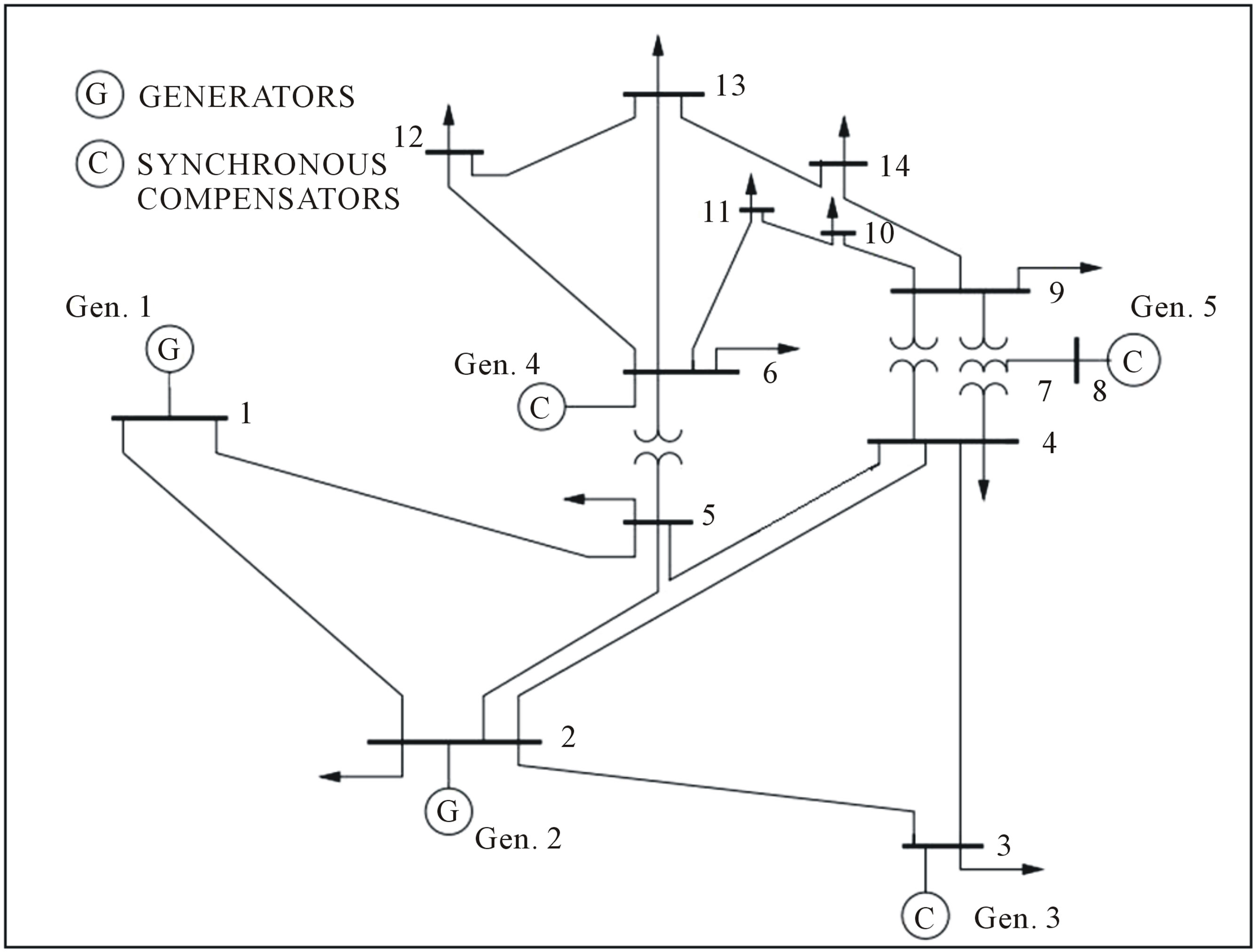
Figure 2: IEEE 14-bus Test System

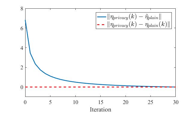
Figure 3: Trajectories of $\|\eta_{privcy}(k)-\tilde{\eta}_{plain}\|$ and $\|\eta_{privcy}(k)-\eta_{plain}(k)\|$

Table 2: Running time of Algorithm 1 on the demand response problem

Key length	average time	maximum time
(bit)	/iter./customer (s)	/iter./customer (s)
500	0.0097	0.0099
1000	0.0100	0.0102
2000	0.0101	0.0103
3000	0.0104	0.0105
4000	0.0110	0.0112

6.2 Algorithm 2

We next simulate Algorithm 2 by an optimal power flow (OPF) problem.

6.2.1 Optimal power flow problem

$\bullet$ Problem formulation. Consider a power network comprising a set of agents $\mathcal{V}\buildrel\Delta\over{=}\{1,\cdots,N\}$ and a system operator. In an OPF setting, the agents could be power generators who supply electric energy via reference buses and the system operator could be an energy manager responsible for power supply regulation. For each generator $i$, let $\mathcal{N}_{i}\subseteq\mathcal{V}$ identify the set of neighbors to generator $i$. We adopt the OPF model from page 514 of Wood and Wollenberg (1996) with the simplification that each bus has only one generator and one load. The physical meanings of the parameters and variables of the OPF problem are listed in Table 3. The OPF problem is formulated as follows:

$$\!\!\!\!\!\!\!\!\!\!\!\mathop{\min}\nolimits_{P\in[\underline{P},\overline{P}],\theta\in{\mathbb{R}^{N}}}\sum\nolimits_{i\in\mathcal{V}}{(a_{i}P_{i}^{2}+b_{i}P_{i})}$$

$${\rm{s.t.}}\,\, {P_{{i}}}-L_{i}=D_{i}\tilde{\omega}+\sum\nolimits_{j\in\mathcal{N}_{i}}t_{ij}(\theta_{i}-\theta_{j}),\,\forall i\in\mathcal{V},$$

$$t_{ij}(\theta_{i}-\theta_{j})\leq{\overline{P}_{ij}},\,\forall j\in\mathcal{N}_{i},\,\forall i\in\mathcal{V}$$ (7)

where $a_{i}>0$ for all $i\in\mathcal{V}$, $P=(P_{i})\in\mathbb{R}^{N}$, $\theta=(\theta_{i})\in\mathbb{R}^{N}$, and $\tilde{\omega}=60{\rm Hz}$ is the steady state of $\omega$. In problem (6.2.1), the objective function measures the power losses or the cost of supplied power. The equality constraints represent the power balance between neighboring reference buses. The inequality constraints depict the capacity limit of a line connecting two neighboring buses.

Table 3: Parameters/variables of the OPF problem

$a,b$	cost parameters
$\omega$	angular frequency
$\theta$	phase angle
$P$	mechanical power
$\underline{P}$	lower limit of mechanical power
$\overline{P}$	upper limit of mechanical power
$L$	power load
$\overline{P}_{ij}$	capacity of line connecting buses $i$ and $j$
$D$	load-damping constant
$t_{ij}$	tie-line stiffness coefficient

Notice that each summand of the objective function of (6.2.1), $a_{i}P_{i}^{2}+b_{i}P_{i}$, only depends on and is convex in generator $i$’s local state $P_{i}$ and the constraints of problem (6.2.1) are affine in $(P_{i},\theta_{i})$. Thus, problem (6.2.1) is separable and equivalent to the distributed optimization problem where, given $(P_{{-i}},\theta_{-i})$, each generator $i$ aims to solve the following optimization problem:

$$\!\!\!\!\!\!\!\!\!\!\!\mathop{\min}\nolimits_{P_{i}\in[\underline{P}_{i},\overline{P}_{i}],\theta_{i}\in{\mathbb{R}}}\,\,a_{i}P_{i}^{2}+b_{i}P_{i}$$

$${\rm{s.t.}}\,\, {P_{{\ell}}}-L_{\ell}=D_{\ell}\tilde{\omega}+\sum\limits_{j\in\mathcal{N}_{\ell}}t_{\ell j}(\theta_{\ell}-\theta_{j}),\;\forall\ell\in\mathcal{N}_{i}\cup\{i\},$$

$$\!\!\!\!\!t_{ij}(\theta_{i}-\theta_{j})\leq{\overline{P}_{ij}},\,\,t_{ji}(\theta_{j}-\theta_{i})\leq{\overline{P}_{ji}},\;\forall j\in\mathcal{N}_{i}.$$ (8)

$\bullet$ Derivation of update rule (1). Denote by $\lambda_{\ell}$ for $\ell\in\mathcal{N}_{i}\cup\{i\}$, $\mu_{ij}$ and $\mu_{ji}$ for $j\in\mathcal{N}_{i}$ the dual variables associated with the set of equality constraints, the first set of inequality constraints and the second set of inequality constraints of (6.2.1), respectively. To reduce the computational burden and the accessible amount of information of each generator, we let each generator $i$ hold and update $(P_{i},\theta_{i},\lambda_{i},\mu_{ij},j\in\mathcal{N}_{i})$ (so that $\lambda_{j}$ and $\mu_{ji}$ for each $j\in\mathcal{N}_{i}$ are not held or updated by generator $i$, but by generator $j$). By introducing Lagrange multipliers and applying the projected gradient method, we can derive the update rule in the form of problem (1) as follows:

$$P_{i}(k+1)=\mathbb{P}_{[\underline{P}_{i},\overline{P}_{i}]}[P_{i}(k)-\gamma(k)(2a_{i}P_{i}(k)+b_{i}$$

$$\qquad\qquad\quad\,-\lambda_{i}(k))]$$

$$\theta_{i}(k+1)=\theta_{i}(k)-\gamma(k)\sum\nolimits_{j\in\mathcal{N}_{i}}(t_{ij}(\lambda_{i}(k)+\mu_{ij}(k))$$

$$\qquad\qquad\quad\,-t_{ij}(\lambda_{j}(k)+\mu_{ji}(k)))$$

$$\lambda_{i}(k+1)=\lambda_{i}(k)+\gamma(k)(L_{i}-P_{i}(k)+D_{i}\tilde{\omega}$$

$$\qquad\qquad\quad\,+\sum\nolimits_{j\in\mathcal{N}_{i}}t_{ij}(\theta_{i}(k)-\theta_{j}(k)))$$

$$\mu_{ij}(k+1)=\mathbb{P}_{\mathbb{R}_{\geq 0}}[\mu_{ij}(k)+\gamma(k)(t_{ij}(\theta_{i}-\theta_{j})-{\overline{P}_{ij}})].$$

$\bullet$ Privacy issue. Each generator $i$ holds its primal and dual variables $(P_{i},\theta_{i},\lambda_{i},\mu_{ij},j\in\mathcal{N}_{i})$ and the coefficients $(a_{i},b_{i},L_{i},\overline{P}_{i},\underline{P}_{i})$, whose values should be kept private to generator $i$. Otherwise, an adversary who knows the current power system state could infer a critical contingency and launch a targeted attack to implement it Dán et al. (2013). On the other hand, the energy manager (the system operator) holds the line-dependent coefficients $(\overline{P}_{ij},D_{i},t_{ij})$ whose values should be kept private to the energy manager. In power systems, the line-dependent coefficients are often very important to the system operator for security consideration. Leaks of these coefficients could be financially damaging and cause potential threat to national security Borden et al. (2013), Borden et al. (2012). For example, an adversary could leverage such information to infer expected congestion in the power system and use this knowledge for insider trading in the power markets Dán et al. (2013).

6.2.2 Simulation results

We use the IEEE 37-bus Test System Report (1991), shown by Fig. 4, as the OPF network. The values of the parameters are chosen as follows: for all $i\in\mathcal{V}$, $D_{i}=1MW/Hz$, $t_{ij}=1.5MW/rad$, $a_{i}=0.1$, $b_{i}=10$, $\overline{P}_{i}=100MW$, $\underline{P}_{i}=10MW$, $P_{L_{i}}=10MW$ and $\overline{P}_{ij}=80MW$. We tested different lengths of keys and have checked that Assumption 4.2 is satisfied for all the tested cases.

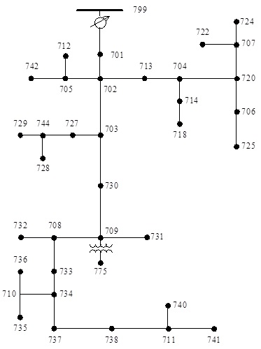
Figure 4: IEEE 37-bus Test System

$\bullet$ Perfect correctness. We stack the collective primal and dual variables $(P,\theta,\lambda,\mu)$ into a single column vector $\eta$. Similar simulation process of Algorithm 1 is performed here. Fig. 5 shows the trajectories of $\|\eta_{privacy}(k)-\tilde{\eta}_{plain}\|$ and $\|\eta_{privacy}(k)-\eta_{plain}(k)\|$, which verify the perfect correctness of Algorithm 2.

$\bullet$ Computational efficiency. The running time is shown by Table 4. The first column is the length of the public key $\alpha_{i}$’s in bit. The average and maximum time per iteration per generator in the second and third columns consists of a single generator’s encryption, encrypted computation, decryption, transformation between real numbers and integers and local update for a single iteration. Table 2 shows that the proposed public key secure computation algorithm can be efficiently implemented.

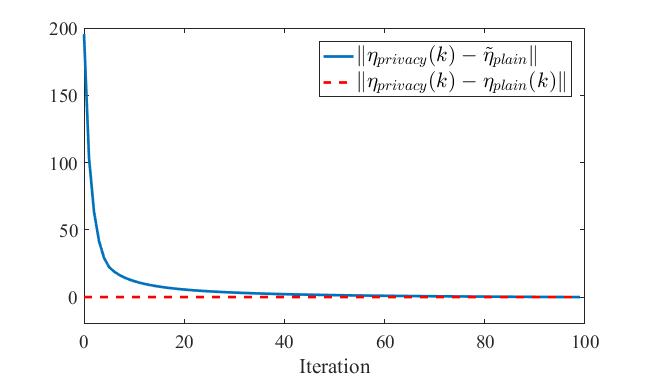
Figure 5: Trajectories of $\|\eta_{privacy}(k)-\tilde{\eta}_{plain}\|$ and $\|\eta_{privacy}(k)-\eta_{plain}(k)\|$

Table 4: Running time of Algorithm 2 on the OPF problem

Key length	average time	maximum time
(bit)	/iter./generator (s)	/iter./generator (s)
500	0.0147	0.0193
1000	0.0424	0.0461
2000	0.2168	0.2492
3000	0.6825	0.7461
4000	1.5487	1.7259

7 Proofs

In this section, we provide the proofs of the theoretical results derived in the previous sections.

7.1 Proof of Theorem 3.1

1) Proof of correctness.

We first fix a step $k$ and some $I\in\mathcal{V}$ and $J\in\{1,\cdots,n_{I}\}$ to show that $\hat{\Phi}_{IJ}^{s}(k)=\Phi_{IJ}(x(k))$. Recall that $10^{\sigma}x(k)$ and $10^{\sigma}c$ are both integer vectors.

For each $\ell=1,\cdots,\kappa_{IJ}$, $Q_{IJ}^{\ell}(\hat{x}(k),\hat{y})$ is a monomial evaluated at $(\hat{x}(k),\hat{y})$. Since $\hat{y}_{\rm SO}=10^{\sigma}c_{\rm SO}$ and, for each $i\in\mathcal{V}$, $\hat{y}_{i}=u_{y_{i}}w+10^{\sigma}c_{i}$ and $\hat{x}_{i}(k)=u_{x_{i}}(k)w+10^{\sigma}x_{i}(k)$, $Q_{IJ}^{\ell}(\hat{x}(k),\hat{y})$ can be expressed as

$$\!\!\!\!\!Q_{IJ}^{\ell}(\hat{x}(k),\hat{y})=\psi_{IJ}^{\ell}(k)w+10^{{\rm deg}(Q_{IJ}^{\ell})\sigma}Q_{IJ}^{\ell}(x(k),c)$$ (9)

where $\psi_{IJ}^{\ell}(k)$ is an integer. To see this, consider the example $Q_{IJ}^{\ell}(x,y)=y_{I}x_{I}$, where $y_{I}$ and $x_{I}$ are assumed to be scalars for simplicity. Then, ${\rm deg}(Q_{IJ}^{\ell})=2$. We have

$$Q_{IJ}^{\ell}(\hat{x}(k),\hat{y})=\hat{y}_{I}\hat{x}_{I}(k)$$

$$=(u_{y_{I}}w+10^{\sigma}c_{I})(u_{x_{I}}(k)w+10^{\sigma}x_{I}(k))$$

$$=(u_{y_{I}}u_{x_{I}}(k)w+10^{\sigma}(x_{I}(k)u_{y_{I}}+c_{I}u_{x_{I}}(k)))w$$

$$\quad+10^{2\sigma}c_{I}x_{I}(k)=\psi_{IJ}^{\ell}(k)w+10^{{\rm deg}(Q_{IJ}^{\ell})\sigma}Q_{IJ}^{\ell}(x(k),c)$$

where $\psi_{IJ}^{\ell}(k)=u_{y_{I}}u_{x_{I}}(k)w+10^{\sigma}(x_{I}(k)u_{y_{I}}+c_{I}u_{x_{I}}(k))$. By (9), for each $\ell=1,\cdots,\kappa_{IJ}$, we then have

$$10^{({\rm deg}(\Phi_{IJ}^{s})-{\rm deg}(Q_{IJ}^{\ell}))\sigma}Q_{IJ}^{\ell}(\hat{x}(k),\hat{y})$$

$$=\rho_{IJ}^{\ell}(k)w+10^{{\rm deg}(\Phi_{IJ}^{s})\sigma}Q_{IJ}^{\ell}(x(k),c)$$ (10)

where $\rho_{IJ}^{\ell}(k)=10^{({\rm deg}(\Phi_{IJ}^{s})-{\rm deg}(Q_{IJ}^{\ell}))\sigma}\psi_{IJ}^{\ell}(k)$ is an integer. By (7.1), we can further obtain

$$\bar{\Phi}_{IJ}^{s}(k)=\sum\nolimits_{\ell=1}^{\kappa_{IJ}}[10^{({\rm deg}(\Phi_{IJ}^{s})-{\rm deg}(Q_{IJ}^{\ell}))\sigma}Q_{IJ}^{\ell}(\hat{x}(k),\hat{y})]$$

$$=w\sum\nolimits_{\ell=1}^{\kappa_{IJ}}{\rho_{IJ}^{\ell}(k)}+10^{{\rm deg}(\Phi_{IJ}^{s})\sigma}\sum\nolimits_{\ell=1}^{\kappa_{IJ}}Q_{IJ}^{\ell}(x(k),c)$$

$$=\varsigma_{IJ}(k)w+10^{{\rm deg}(\Phi_{IJ}^{s})\sigma}\Phi_{IJ}(x(k))$$ (11)

where $\varsigma_{IJ}(k)=\sum\nolimits_{\ell=1}^{\kappa_{IJ}}{\rho_{IJ}^{\ell}(k)}$ is an integer. By (7.1)

$$\bar{\Phi}_{IJ}^{s}(k)\!\!\mod w=10^{{\rm deg}(\Phi_{IJ}^{s})\sigma}\Phi_{IJ}(x(k))\!\!\mod w.$$ (12)

By Assumption 3.1, $|10^{{\rm deg}(\Phi_{IJ}^{s})\sigma}\Phi_{IJ}(x(k))|<{(w-1)}/{2}$. By Lemma 2.1, we then have $\hat{\Phi}_{IJ}^{s}(k)=T_{{\rm deg}(\Phi_{IJ}^{s})\sigma,w}$ $(10^{{\rm deg}(\Phi_{IJ}^{s})\sigma}\Phi_{IJ}(x(k))\mod w)=\Phi_{IJ}(x(k))$. The above analysis holds for $\Phi_{ij}(x(k))$ for any $k$ and $(i,j)$. Hence, for each $k$ and $i\in\mathcal{V}$, we have $\hat{\Phi}_{i}^{s}(k)=\Phi_{i}(x(k))$.

2) Proof of security.

The security proof adopts the simulation paradigm which is a standard technique for proving SMC Cramer et al. (2015), Lindell and Pinkas (2009). First we show by Definition 2.2 that Algorithm 1 securely computes $\{\Phi_{1}(x(k)),\cdots,\Phi_{N}(x(k))\}$ between the agents. During each step $k$ of the execution of Algorithm 1, for each $i\in\mathcal{V}$, agent $i$ only receives $\bar{\Phi}_{i}^{s}(k)$. Thus, the view of agent $i$ during step $k$ of Algorithm 1 is ${\rm VIEW}_{i}(k)=\{x_{i}(k),C_{\Phi}^{i},X_{i},\sigma,w,u_{x_{i}}(k),u_{y_{i}},\bar{\Phi}_{i}^{s}(k),$ $\Phi_{i}(x(k))\}$, where $x_{i}(k)$, $C_{\Phi}^{i}$, $X_{i}$, $\sigma$, $w$, $u_{x_{i}}(k)$ and $u_{y_{i}}$ are inputs of agent $i$ and $\Phi_{i}(x(k))$ is agent $i$’s output which can be inferred from $\bar{\Phi}_{i}^{s}(k)$ by the correctness analysis. We need to construct an algorithm $S$ by which, for each $i\in\mathcal{V}$, given agent $i$’s inputs $\{x_{i}(k),C_{\Phi}^{i},X_{i},\sigma,w,u_{x_{i}}(k),u_{y_{i}}\}$ and output $\Phi_{i}(x(k))$, agent $i$ can generate a set of data $S(i,k)$ such that $S(i,k)\mathop{\equiv}\limits^{c}{\rm VIEW}_{i}(k)$. Agent $i$ then only has to simulate $\bar{\Phi}_{i}^{s}(k)$, i.e., to generate $\bar{\Phi}_{i}^{s}(k)^{\prime}$ by $S$ such that $\{\bar{\Phi}_{i}^{s}(k)^{\prime}\}\mathop{\equiv}\limits^{c}\{\bar{\Phi}_{i}^{s}(k)\}$. By (7.1), we have $\bar{\Phi}_{ij}^{s}(k)=\varsigma_{ij}(k)w+10^{{\rm deg}(\Phi_{ij}^{s})\sigma}\Phi_{ij}(x(k))$. Since each agent $\ell$ randomly chooses $u_{x_{\ell}}(k)$ and $u_{y_{\ell}}$, $\varsigma_{ij}(k)$ is a random number to agent $i$. Let $\bar{c}_{i}$ and $\bar{c}_{-i}$ be the vectors of the elements of $C_{\Phi}^{i}$ and $C_{\Phi}\backslash C_{\Phi}^{i}$, respectively. Agent $i$ simulates $\bar{\Phi}_{i}^{s}(k)$ as follows. First, agent $i$ generates $x_{-i}(k)^{\prime}$ and $\bar{c}_{-i}^{\prime}$ such that $\Phi_{i}^{s}(x_{i}(k),x_{-i}(k)^{\prime},\bar{c}_{i},\bar{c}_{-i}^{\prime})=\Phi_{i}(x(k))$. Then, agent $i$ randomly chooses $(u_{x_{-i}}(k)^{\prime},u_{y_{-i}}^{\prime})$ following the same distribution as $(u_{x_{-i}}(k),u_{y_{-i}})$ and computes $\hat{x}_{i}(k)=u_{x_{i}}(k)w+x_{i}(k)$, $\hat{y}_{i}=u_{y_{i}}w+\bar{c}_{i}$, $\hat{x}_{-i}(k)^{\prime}=u_{x_{-i}}(k)^{\prime}w+x_{-i}(k)^{\prime}$ and $\hat{y}_{-i}^{\prime}=u_{y_{-i}}^{\prime}w+\bar{c}_{-i}^{\prime}$. Agent $i$ then computes $\bar{\Phi}_{i}^{s}(k)^{\prime}$ in the same way as that of line 6 of Algorithm 1 by using $\{\hat{x}_{i}(k),\hat{x}_{-i}(k)^{\prime},\hat{y}_{i},\hat{y}_{-i}^{\prime}\}$. By the same arguments in the correctness analysis part, we have $\bar{\Phi}_{ij}^{s}(k)^{\prime}=\varsigma_{ij}(k)^{\prime}w+10^{{\rm deg}(\Phi_{ij}^{s})\sigma}\Phi_{ij}(x(k))$, where $\varsigma_{ij}(k)^{\prime}$ is an integer which has the same distribution with $\varsigma_{ij}(k)$. Thus, we have $\{\bar{\Phi}_{i}^{s}(k)^{\prime}\}\mathop{\equiv}\limits^{c}\{\bar{\Phi}_{i}^{s}(k)\}$. By Definition 2.2, Algorithm 1 securely computes $\{\Phi_{1}(x(k)),\cdots,\Phi_{N}(x(k))\}$ between the agents.

Next we show that Algorithm 1 is as hard as the approximate GCD problem for the system operator to solve $x(k)$ and $c_{\mathcal{V}}$ at each step $k$. Under Assumption 3.2, at each step $k$, the system operator knows $\hat{x}(k)=u_{x}(k)w+10^{\sigma}x(k)$ and $\hat{y}=u_{y}w+10^{\sigma}c_{\mathcal{V}}$. To infer $x(k)$ and $c_{\mathcal{V}}$ from $\hat{x}(k)$ and $\hat{y}$, the system operator has to recover the value of $w$, which is exactly the approximate GCD problem.

7.2 Proof of Theorem 4.1

1) Proof of correctness.

For each step $k$ and compatible $(i,\ell)$, since $\bar{\Phi}_{i\ell}^{s}(k)=(\beta_{i}^{10^{2\sigma}B_{i\ell}\mod\alpha_{i}}\prod\nolimits_{j=1}^{N}\prod\nolimits_{v=1}^{n_{j}}\hat{x}_{jv}^{i}(k)^{10^{\sigma}A_{i\ell}^{jv}\mod\alpha_{i}})\mod$ $\alpha_{i}^{2}$, by (3) of Theorem 9.1, we have $\frac{(\bar{\Phi}_{i\ell}^{s}(k)^{\nu}\mod\alpha_{i}^{2})-1}{\alpha_{i}}\cdot\pi_{i}\mod\alpha_{i}=10^{2\sigma}(A_{i\ell}x(k)+B_{i\ell})\mod\alpha_{i}$. By Assumption 4.2, $10^{2\sigma}|A_{i\ell}x(k)+B_{i\ell}|\leq(\alpha_{i}-1)/2$. By Lemma 2.1, we have $\hat{\Phi}_{i\ell}^{s}(k)=T_{2\sigma,\alpha_{i}}(10^{2\sigma}(A_{i\ell}x(k)+B_{i\ell})\mod\alpha_{i})=A_{i\ell}x(k)+B_{i\ell}=\Phi_{i\ell}(x(k))$. The above analysis holds for any step $k$ and any pair $(i,\ell)$. Hence, for each step $k$ and each $i\in\mathcal{V}$, we have $\hat{\Phi}_{i}^{s}(k)=\Phi_{i}(x(k))$.

2) Proof of security.

We first show by Definition 2.2 that Algorithm 2 securely computes $\{\Phi_{1}(x(k)),\cdots,\Phi_{N}(x(k))\}$ between the agents. During each step $k$ of the execution of Algorithm 2, for each $i\in\mathcal{V}$, agent $i$ only receives $\bar{\Phi}_{i}^{s}(k)$ and ${\rm VIEW}_{i}(k)=\{x_{i}(k),\sigma,\alpha_{i},\beta_{i},\nu_{i},\pi_{i},\bar{\Phi}_{i}^{s}(k),\Phi_{i}(x(k))\}$. We need to construct an algorithm $S$ by which, given agent $i$’s inputs $\{x_{i}(k),\sigma,\alpha_{i},\beta_{i},\nu_{i},\pi_{i}\}$ and output $\Phi_{i}(x(k))$, agent $i$ can generate a set of data $S(i,k)$ such that $S(i,k)\mathop{\equiv}\limits^{c}{\rm VIEW}_{i}(k)$. Again, agent $i$ only has to generate $\bar{\Phi}_{i}^{s}(k)^{\prime}$ by $S$ such that $\{\bar{\Phi}_{i}^{s}(k)^{\prime}\}\mathop{\equiv}\limits^{c}\{\bar{\Phi}_{i}^{s}(k)\}$. Agent $i$ simulates $\bar{\Phi}_{i}^{s}(k)$ as follows. First, agent $i$ generates $x_{-i}(k)^{\prime}$ and $(A_{i}^{\prime},B_{i}^{\prime})$ such that $\Phi_{i}^{s}(x_{i}(k),x_{-i}(k)^{\prime},A_{i}^{\prime},B_{i}^{\prime})$ $=\Phi_{i}(x(k))$. Then, for each $j\in\mathcal{V}\backslash\{i\}$, agent $i$ randomly chooses $r_{j}(k)^{\prime}$ where each $r_{j\ell}(k)^{\prime}\in\mathbb{Z}_{\alpha_{i}}^{*}$ and encrypts $x_{j}(k)^{\prime}$ by line 4 of Algorithm 2 to obtain $\hat{x}_{j}(k)^{\prime}$. Then, agent $i$ computes $\bar{\Phi}_{i}^{s}(k)^{\prime}$ in the same way as line 5 of Algorithm 2 by using $(\hat{x}_{i}(k),\hat{x}_{-i}(k)^{\prime},A_{i}^{\prime},B_{i}^{\prime})$. For each $j=1,\cdots,n_{i}$, by (3) of Theorem 9.1, we have that $\bar{\Phi}_{ij}^{s}(k)^{\prime}$ satisfies the decryption correctness, i.e., $\frac{(\bar{\Phi}_{ij}^{s}(k)^{\prime\nu}\mod\alpha_{i}^{2})-1}{\alpha_{i}}\cdot\pi_{i}\mod\alpha_{i}=10^{2\sigma}\Phi_{ij}(x(k))\mod\alpha_{i}$. Hence, $\{\bar{\Phi}_{i}^{s}(k)^{\prime}\}\mathop{\equiv}\limits^{c}\{\bar{\Phi}_{i}^{s}(k)\}$. By Definition 2.2, Algorithm 2 securely computes $\{\Phi_{1}(x(k)),\cdots,\Phi_{N}(x(k))\}$ between the agents.

We next show that Algorithm 2 is semantically secure against the system operator. During the execution of Algorithm 2, at each step $k$, the system operator receives $N$ encrypted vectors of $x(k)$, each one encrypted by a different set of Paillier keys. By Theorem 9.1, the Paillier encryption scheme is semantically secure for encrypting a plaintext a single time. Then, by Theorem 5.2.10 of Goldreich (2004), the Paillier encryption scheme is also semantically secure for encrypting a message $N$ times by different keys against an adversary who knows all the $N$ ciphertexts. Denote by $E(\cdot)$ the encryption operator of Algorithm 2. By Definition 2.3, to the system operator, $E(x)\mathop{\equiv}\limits^{c}E(x^{\prime})$ for any plaintexts $x,x^{\prime}$ even if the system operator knows $x$ and $x^{\prime}$. Thus, to the system operator, $E(x(k))\mathop{\equiv}\limits^{c}E(x(k+\kappa))$ for any $k$ and any $\kappa$ even if the system operator knows $x(k)$ and $x(k+\kappa)$ or any relation between $x(k)$ and $x(k+\kappa)$. Hence, even if the system operator knows the update rule of $x(k)$ and launchs causal attacks, Algorithm 2 is still semantically secure. This establishes the semantic security of Algorithm 2.

7.3 Proof of Theorem 5.1

We focus on an adversary $i\in\mathcal{V}$. By Definition 2.4, we are to show that agent $i$ cannot uniquely determine $(\{x_{-i}(0),\cdots,x_{-i}(K)\},X_{-i},[B_{j\ell}]_{(j,\ell)\in\Omega_{i}^{\prime}})$ and the uncertainty is unbounded for any $K\in\mathbb{N}$. For each $j\in\mathcal{V}$ and $\ell=1,\cdots,n_{j}$, denote the true $(X_{j\ell},B_{j\ell},\{x_{j\ell}(0),\cdots,x_{j\ell}(K)\})$ by $(\bar{X}_{j\ell},\bar{B}_{j\ell},\{\bar{x}_{j\ell}(0),$ $\cdots,\bar{x}_{j\ell}(K)\})$. Up to step $k$, agent $i$ knows $\bar{X}_{i}$, $H_{j\ell}$ and $A_{j\ell}$ for all $j\in\mathcal{V}$ and $\ell\in\{1,\cdots,n_{j}\}$, $B_{j\ell}$ for $(j,\ell)\in\Omega_{i}$, the sequences $\{\bar{x}_{i}(0),\cdots,\bar{x}_{i}(k)\}$, $\{\Phi_{i}(\bar{x}(0)),\cdots,\Phi_{i}(\bar{x}(k))\}$ and $\{\gamma(0),\cdots,\gamma(k)\}$. For convenience of notation, let $\hat{x}_{i}(k)=\bar{x}_{i}(k)$ for all $k\in\{0,\cdots,K\}$. We aim to find $(\hat{X}_{-i},\{\hat{x}_{-i}(0),\cdots,\hat{x}_{-i}(K)\},$ $[\hat{B}_{j\ell}]_{(j,\ell)\in\Omega_{i}^{\prime}})$ which satisfy the following constraints:

$$\hat{x}_{j\ell}(k+1)=\mathbb{P}_{\hat{X}_{j\ell}}[\hat{x}_{j\ell}(k)-\gamma(k)\hat{x}(k)^{T}H_{j\ell}\hat{x}(k)$$

$$+A_{j\ell}\hat{x}(k)+\bar{B}_{j\ell})],\;\forall(j,\ell)\in\Omega_{i},\;j\neq i,$$

$$\ell\in\{1,\cdots,n_{j}\},\;k\in\{0,\cdots,K-1\},$$ (13)

$$\hat{x}_{j\ell}(k+1)=\mathbb{P}_{\hat{X}_{j\ell}}[\hat{x}_{j\ell}(k)-\gamma(k)\hat{x}(k)^{T}H_{j\ell}\hat{x}(k)$$

$$+A_{j\ell}\hat{x}(k)+\hat{B}_{j\ell})],\;\forall(j,\ell)\in\Omega_{i}^{\prime},\;j\neq i,$$

$$\ell\in\{1,\cdots,n_{j}\},\;k\in\{0,\cdots,K-1\},$$ (14)

$$\!\!\!\!\!\!\left\{{\begin{array}[]{*{20}{l}}\Phi_{i\ell}(\bar{x}(k))=\hat{x}(k)^{T}H_{i\ell}\hat{x}(k)+A_{i\ell}\hat{x}(k)+\bar{B}_{i\ell},\\ \forall k\in\{0,\cdots,K\},\;\ell\in\{1,\cdots,n_{i}\},\;{\rm if}\;(i,\ell)\in\Omega_{i},\\ \Phi_{i\ell}(\bar{x}(k))=\hat{x}(k)^{T}H_{i\ell}\hat{x}(k)+A_{i\ell}\hat{x}(k)+\hat{B}_{i\ell},\\ \forall k\in\{0,\cdots,K\},\;\ell\in\{1,\cdots,n_{i}\},\;{\rm if}\;(i,\ell)\in\Omega_{i}^{\prime}.\end{array}}\right.$$ (19)

Consider the following construction: $\hat{x}_{j}(k)=\bar{x}_{j}(k)+\delta_{j}$ for each $j\in\mathcal{V}$ and each $k\in\{0,\cdots,K\}$, where $\delta_{i}=0$, and for each $j\neq i$, $\delta_{j}\in\mathbb{R}^{n_{j}}$ is an arbitrary constant vector such that each entry of each $\delta_{j}$ is nonzero and $[(H^{-i})^{T},(A^{-i})^{T}]^{T}\delta_{-i}=0$, with $\delta_{-i}=[\delta_{v}]_{v\neq i}$; $\hat{X}_{j}=\{x_{j}+\delta_{j}:x_{j}\in\bar{X}_{j}\}$ for each $j\neq i$; $\hat{B}_{j\ell}=\bar{B}_{j\ell}-A_{j\ell}\delta$ for each $(j,\ell)\in\Omega_{i}^{\prime}$ with $\delta=[\delta_{v}]_{v\in\mathcal{V}}$. Assumption 5.2 guarantees the existence of the above set of $\delta_{j}$’s. By the definition of $H^{-i}$ and $A^{-i}$ given in the fourth paragraph of Section 5, we have $(H_{j\ell}^{uv}+(H_{j\ell}^{vu})^{T})\delta_{v}=0$ for all possible quadruples $(j,\ell,u,v)$, and $A_{j\ell}\delta=0$ for all $(j,\ell)\in\Omega_{i}$.

First we consider the case where $j\neq i$ and $(j,\ell)\in\Omega_{i}$. By this construction, for each step $k$, it holds that:

$$\mathbb{P}_{\hat{X}_{j\ell}}[\hat{x}_{j\ell}(k)-\gamma(k)(\hat{x}(k)^{T}H_{j\ell}\hat{x}(k)+A_{j\ell}\hat{x}(k)+\bar{B}_{j\ell})]$$

$$=\mathbb{P}_{\hat{X}_{j\ell}}[\bar{x}_{j\ell}(k)+\delta_{j\ell}-\gamma(k)(\sum\nolimits_{u,v=1}^{N}(\bar{x}_{u}(k)+\delta_{u})^{T}$$

$$H_{j\ell}^{uv}(\bar{x}_{v}(k)+\delta_{v})+\sum\nolimits_{v=1}^{N}A_{j\ell}^{v}(\bar{x}_{v}(k)+\delta_{v})+\bar{B}_{j\ell})]$$

$$=\mathbb{P}_{\hat{X}_{j\ell}}[\bar{x}_{j\ell}(k)+\delta_{j\ell}-\gamma(k)(\bar{x}(k)^{T}H_{j\ell}\bar{x}(k)+A_{j\ell}\bar{x}(k)+$$

$$\bar{B}_{j\ell}+\sum\limits_{u,v=1}^{N}(\bar{x}_{u}(k)+\frac{1}{2}\delta_{u})^{T}(H_{j\ell}^{uv}+(H_{j\ell}^{vu})^{T})\delta_{v}+A_{j\ell}\delta)]$$

$$=\mathbb{P}_{\hat{X}_{j\ell}}[\bar{x}_{j\ell}(k)+\delta_{j\ell}-\gamma(k)(\bar{x}(k)^{T}H_{j\ell}\bar{x}(k)+A_{j\ell}\bar{x}(k)$$

$$+\bar{B}_{j\ell})]=\bar{x}_{j\ell}(k+1)+\delta_{j\ell}=\hat{x}_{j\ell}(k+1),$$

$$\forall(j,\ell)\in\Omega_{i},\;j\neq i,\;\ell\in\{1,\cdots,n_{j}\}.$$ (20)

Next we consider the case where $j\neq i$ and $(j,\ell)\in\Omega_{i}^{\prime}$. By the above construction, for each step $k$, it holds that:

$$\mathbb{P}_{\hat{X}_{j\ell}}[\hat{x}_{j\ell}(k)-\gamma(k)(\hat{x}(k)^{T}H_{j\ell}\hat{x}(k)+A_{j\ell}\hat{x}(k)+\hat{B}_{j\ell})]$$

$$=\mathbb{P}_{\hat{X}_{j\ell}}[\bar{x}_{j\ell}(k)+\delta_{j\ell}-\gamma(k)(\sum\nolimits_{u,v=1}^{N}(\bar{x}_{u}(k)+\delta_{u})^{T}H_{j\ell}^{uv}$$

$$(\bar{x}_{v}(k)+\delta_{v})+\sum\nolimits_{v=1}^{N}A_{j\ell}^{v}(\bar{x}_{v}(k)+\delta_{v})+\bar{B}_{j\ell}-A_{j\ell}\delta)]$$

$$=\mathbb{P}_{\hat{X}_{j\ell}}[\bar{x}_{j\ell}(k)+\delta_{j\ell}-\gamma(k)(\bar{x}(k)^{T}H_{j\ell}\bar{x}(k)+A_{j\ell}\bar{x}(k)$$

$$+\bar{B}_{j\ell}+\sum\limits_{u,v=1}^{N}(\bar{x}_{u}(k)+\frac{1}{2}\delta_{u})^{T}(H_{j\ell}^{uv}+(H_{j\ell}^{vu})^{T})\delta_{v})]$$

$$=\mathbb{P}_{\hat{X}_{j\ell}}[\bar{x}_{j\ell}(k)+\delta_{j\ell}-\gamma(k)(\bar{x}(k)^{T}H_{j\ell}\bar{x}(k)+A_{j\ell}\bar{x}(k)$$

$$+\bar{B}_{j\ell})]=\bar{x}_{j\ell}(k+1)+\delta_{j\ell}=\hat{x}_{j\ell}(k+1),$$

$$\forall(j,\ell)\in\Omega_{i}^{\prime},\;j\neq i,\;\ell\in\{1,\cdots,n_{j}\}.$$ (21)

We next consider the case where $(i,\ell)\in\Omega_{i}$. By the above construction, for each step $k$, it holds that:

$$\hat{x}(k)^{T}H_{i\ell}\hat{x}(k)+A_{i\ell}\hat{x}(k)+\bar{B}_{i\ell}$$

$$=(\bar{x}(k)+\delta)^{T}H_{i\ell}(\bar{x}(k)+\delta)+A_{i\ell}(\bar{x}(k)+\delta)+\bar{B}_{i\ell}$$

$$=\bar{x}(k)^{T}H_{i\ell}\bar{x}(k)+A_{i\ell}\bar{x}(k)+\bar{B}_{i\ell}$$

$$+\sum\nolimits_{u,v=1}^{N}(\bar{x}_{u}(k)+\frac{1}{2}\delta_{u})^{T}(H_{i\ell}^{uv}+(H_{i\ell}^{vu})^{T})\delta_{v}+A_{i\ell}\delta$$

$$=\bar{x}(k)^{T}H_{i\ell}\bar{x}(k)+A_{i\ell}\bar{x}(k)+\bar{B}_{i\ell}=\Phi_{i\ell}(\bar{x}(k)),$$

$$\forall\ell\in\{1,\cdots,n_{j}\},\;{\rm if}\;(i,\ell)\in\Omega_{i}.$$ (22)

Finally we consider the case where $(i,\ell)\in\Omega_{i}^{\prime}$. By the above construction, for each step $k$, it holds that:

$$\hat{x}(k)^{T}H_{i\ell}\hat{x}(k)+A_{i\ell}\hat{x}(k)+\hat{B}_{i\ell}$$

$$=(\bar{x}(k)+\delta)^{T}H_{i\ell}(\bar{x}(k)+\delta)+A_{i\ell}(\bar{x}(k)+\delta)+\bar{B}_{i\ell}$$

$$-A_{i\ell}\delta=\bar{x}(k)^{T}H_{i\ell}\bar{x}(k)+A_{i\ell}\bar{x}(k)+\bar{B}_{i\ell}$$

$$+\sum\nolimits_{u,v=1}^{N}(\bar{x}_{u}(k)+\frac{1}{2}\delta_{u})^{T}(H_{i\ell}^{uv}+(H_{i\ell}^{vu})^{T})\delta_{v}$$

$$=\bar{x}(k)^{T}H_{i\ell}\bar{x}(k)+A_{i\ell}\bar{x}(k)+\bar{B}_{i\ell}=\Phi_{i\ell}(\bar{x}(k)),$$

$$\forall\ell\in\{1,\cdots,n_{j}\},\;{\rm if}\;(i,\ell)\in\Omega_{i}^{\prime}.$$ (23)

It is easy to see that (7.3) implies (7.3), (7.3) implies (7.3), and (7.3) and (7.3) imply (19). Thus, the above construction of $(\{\hat{x}_{-i}(0),\cdots,\hat{x}_{-i}(K)\},\hat{X}_{-i},[\hat{B}_{j\ell}]_{(j,\ell)\in\Omega_{i}^{\prime}})$ satisfies (7.3), (7.3) and (19). By the definition of $\Delta_{j}^{i}$ in Definition 2.4, we have $(\{\hat{x}_{j}(0),\cdots,\hat{x}_{j}(K)\},\hat{X}_{j},[\hat{B}_{j\ell}]_{(j,\ell)\in\Omega_{i}^{\prime}})\in\Delta_{j}^{i}(\{\bar{x}(0),\cdots,\bar{x}(K)\},\bar{X},\bar{B})$ for each $j\neq i$. Fix any set of $\delta_{j}$’s constructed above. Then for an arbitrary nonzero real number $r$, $r\delta$ also satisfies the condition given in Assumption 5.2, i.e., $[(H^{-i})^{T},(A^{-i})^{T}]^{T}r\delta_{-i}=0$, and thus the construction of $(\{\hat{x}_{j}(0),\cdots,\hat{x}_{j}(K)\},\hat{X}_{j},\hat{B})$ by replacing $\delta_{j}$ with $r\delta_{j}$ also belongs to $\Delta_{j}^{i}(\{\bar{x}(0),\cdots,\bar{x}(K)\},$ $\bar{X},\bar{B})$. Notice that each entry of each $r\delta_{j}$ is nonzero and could be arbitrarily large by choosing $r$ arbitrarily large. Hence, by the definition of ${\rm Dist}_{j}^{i}$ in Definition 2.4, for each $j\neq i$, we have ${\rm Dist}_{j}^{i}(\{\bar{x}(0),\cdots,\bar{x}(K)\},\bar{X},\bar{B})\geq\sup_{r\in\mathbb{R}}\|r\delta_{j}-\delta_{j}\|_{2}=\infty$. Since the above analysis holds for any $i\in\mathcal{V}$, we have $\min_{i\neq j}{\rm Dist}_{j}^{i}(\{\bar{x}(0),\cdots,\bar{x}(K)\},$ $\bar{X},\bar{B})=\infty$ for any $j\in\mathcal{V}$. By Definition 2.4, the sequence of functions $\{\Phi(x(0)),\cdots,\Phi(x(K))\}$ resists input-output inference with unbounded uncertainty for any $K\in\mathbb{N}$. This completes the proof.

8 Conclusion

This paper studies how to securely execute a class of distributed projected gradient-based algorithms. We propose new homomorphic encryption based schemes which can achieve perfect correctness and simultaneously protect each participant’s states and coefficients from any other participant. We further study the issue of input-output inference for a class of quadratic joint functions. The correctness and computational efficiency of the proposed algorithms are verified by two case studies of power systems, one on a demand response problem and the other on an optimal power flow problem. An interesting future work is to relax the assumption of temporarily independent attacks (Assumption 3.2) for Algorithm 1.

9 Appendix

9.1 Literature review on homomorphic encryption

Table 5: Summary of different types of homomorphic encryption schemes

	Partially homomorphic	Fully homomorphic
Private key	Key dist. prob. exists; Efficiently implementable	Key dist. prob. exists; Efficiently implementable
Public key	No key dist. prob.; Efficiently implementable	No key dist. prob.; Not efficiently implementable

In general, there are two ways to categorize homomorphic encryption schemes. The first way is based on the keys used in the encryption and decryption operations. Roughly speaking, if the same key is used for both encryption and decryption, then the scheme is referred to as a private key homomorphic encryption scheme; if the keys for encryption and decryption are different and it is computationally infeasible to compute the decryption key from the encryption key, then the scheme is referred to as a public key homomorphic encryption scheme.

The second way of categorization is based on the algebraic operations a homomorphic encryption scheme can carry out. If a scheme can only carry out either addition or multiplication operation but cannot simultaneously carry out both, then the scheme is said to be partially homomorphic; if a scheme can simultaneously carry out both addition and multiplication operations, then the scheme is said to be fully homomorphic.

Table 5 summarizes the state-of-the-art of the four types of homomorphic encryption schemes. Private key fully homomorphic (and surely partially homomorphic) encryption schemes can be efficiently implemented but suffer from the fundamental key distribution problem: the message sender and receiver need to share a key which must be kept unknown to any third party. In practice, the key distribution is usually achieved via face-to-face meeting, use of a trusted courier, or sending the key through an existing secure channel. On the other hand, public key homomorphic encryption schemes have the significant advantage of resolving the key distribution problem since the encryption key can be publicized. To the best of our knowledge, all current efficiently implementable public key homomorphic encryption schemes are partially homomorphic, e.g., the RSA scheme Rivest et al. (1978) and the ElGamal scheme ElGamal (1985) are multiplicatively homomorphic, and the Goldwasser–Micali scheme Goldwasser and Micali (1982) and the Paillier scheme Paillier (1999) are additively homomorphic. The first fully public key homomorphic encryption scheme was developed by Gentry in his seminal work Gentry (2009). However, due to that the Gentry fully homomorphic encryption scheme uses lattice and bootstrapping, its implementation is overwhelmingly time-consuming. Benchmark implementations include: Gentry et al. (2012) reported an AES (Advanced Encryption Standard) encryption on a supercomputer which took 36 hours; in Gentry and Halevi (2011), bootstrapping ranged from 30 seconds for small setting to 30 minutes for large setting. The current lack of efficient implementations largely limits the applications of the Gentry fully homomorphic encryption scheme Armknecht et al. (2015).

9.2 Preliminaries for the Paillier encryption scheme

In this subsection, we provide some preliminaries for the Paillier encryption scheme. The results of this subsection can be found in Paillier (1999) and Yi et al. (2014).

Consider a scenario consisting of a message sender, a message receiver and an adversary. The message sender aims to send a private message to the message receiver via an open communication link which is insecure and can be eavesdropped by the adversary. To achieve secure message delivery, the message sender and receiver can adopt some public key encryption scheme. In this paper, we choose the Paillier encryption scheme as our implementing scheme. The standard Paillier encryption scheme consists of key generation, encryption and decryption operations as follows.

$\bullet$ Key generation: The message receiver randomly chooses two large prime numbers $p$ and $q$ such that ${\rm gcd}(pq,(p-1)(q-1))=1$; computes $\alpha=pq$, $\nu={\rm lcm}(p-1,q-1)$; select random integer $\beta\in\mathbb{Z}_{\alpha^{2}}^{*}$ such that the modular multiplicative inverse $\pi=(\frac{(\beta^{\nu}\mod\alpha^{2})-1}{\alpha})^{-1}\mod\alpha$ exists, i.e., $\pi\frac{(\beta^{\nu}\mod\alpha^{2})-1}{\alpha}\equiv 1\mod\alpha$. The public keys are $(\alpha,\beta)$ and the private keys are $(\nu,\pi)$. The message receiver publicizes $(\alpha,\beta)$ while keeps $(\nu,\pi,p,q)$ private to itself.

$\bullet$ Encryption: To encrypt a plaintext $pt\in\mathbb{Z}_{\alpha}$, the message sender selects a random number $r\in\mathbb{Z}_{\alpha}^{*}$ and computes the ciphertext by the encryption operation $E(\cdot)$ as $ct=E(pt,\alpha,\beta,r)=\beta^{pt}\cdot r^{\alpha}\mod\alpha^{2}$. The message sender then sends $ct$ to the message receiver.

$\bullet$ Decryption: To decrypt the ciphertext $ct\in\mathbb{Z}_{\alpha^{2}}$, the message receiver performs the decryption operation $D(\cdot)$ as $\overline{pt}=D(ct,\alpha,\nu,\pi)=\frac{(ct^{\nu}\mod\alpha^{2})-1}{\alpha}\cdot\pi\mod\alpha$.

In cryptography, the security of most public-key encryption schemes are established under certain mathematical assumptions which state that certain mathematical problems are difficult to solve. Specifically, the semantic security of the Paillier encryption scheme is proved under the decisional composite residuosity assumption (DCRA), stated as follows: Given a composite $C$ and an integer $z$, it is computationally intractable to decide whether $z$ is a $C$-residue modulo $C^{2}$ or not, i.e., whether there exists $y$ such that $z=y^{C}\mod C^{2}$.

The correctness, security and homomorphic properties of the Paillier encryption scheme are provided by the following theorem, whose proof is given in Paillier (1999).

Theorem 9.1.

By the Paillier encryption scheme, the following claims hold:

(1) Correctness: $\overline{pt}=pt$.

(2) Semantic security: If the DCRA holds, then the Paillier encryption scheme is semantically secure.

(3) Homomorphic properties:
(3-i) Given any $pt_{1},\cdots,pt_{m}\in\mathbb{N}$. If $\sum_{\ell=1}^{m}pt_{\ell}\in\mathbb{Z}_{\alpha}$, then $D(\prod_{\ell=1}^{m}E(pt_{\ell},\alpha,\beta,r_{\ell}),\alpha,\nu,\pi)=\sum_{\ell=1}^{m}pt_{\ell}$.
(3-ii) Given any $pt_{1},pt_{2}\in\mathbb{N}$. If $pt_{1}pt_{2}\in\mathbb{Z}_{\alpha}$, then $D(E(pt_{1},\alpha,\beta,r)^{pt_{2}},\alpha,\nu,\pi)=pt_{1}pt_{2}$.  

9.3 Numerical examples for Algorithm 1 and Algorithm 2

In this subsection, to help the readers better understand Algorithm 1 and Algorithm 2, we go through their steps using two simple numerical examples.

9.3.1 A numerical example for Algorithm 1

Consider the case of two agents and a system operator. The accuracy level is set as $\sigma=2$. Each agent $i\in\{1,2\}$ has a scalar state $x_{i}\in\mathbb{R}$. The polynomial joint function of agent 1 is $\Phi_{1}(x_{1},x_{2})=c_{1}x_{1}^{2}+c_{2}x_{2}^{2}+c_{3}x_{1}x_{2}+c_{4}x_{1}+c_{5}$, where $c_{1},c_{3},c_{4}\in\mathbb{R}$ are the private coefficients of agent 1, $c_{2},c_{3}\in\mathbb{R}$ are the private coefficients of agent 2, and $c_{5}\in\mathbb{R}$ is the private coefficient of the system operator. Notice that $c_{3}$ is held by both agent 1 and agent 2. Assume that the participants construct a partition of the coefficient set according to Section 3.1 as $\tilde{C}_{\Phi}^{1}=\{c_{1},c_{3},c_{4}\}$, $\tilde{C}_{\Phi}^{2}=\{c_{2}\}$ and $\tilde{C}_{\Phi}^{\rm SO}=\{c_{5}\}$. Assume $c_{1}=3.32$, $c_{2}=-1.53$, $c_{3}=4.67$, $c_{4}=-0.28$, $c_{5}=2.42$, $x_{1}(0)=0.76$, $x_{2}(0)=-2.35$, $X_{1}=\mathbb{R}$ and $\gamma(0)=1$. One can check $\Phi_{1}(x_{1}(0),x_{2}(0))=-12.665213$. We next go through the steps of Algorithm 1 to compute $\Phi_{1}(x_{1}(0),x_{2}(0))$ for one iteration.

1. Initialization: Agent 1 holds $x_{1}(0)=0.76$ and agent 2 holds $x_{2}(0)=-2.35$.

2. Key agreement: Agent 1 and agent 2 agree on a key $w$ according to Assumption 3.1 and keep it secret from the system operator. We have $1+2\times 10^{{\rm deg}(\Phi_{1}^{s})\sigma}|\Phi_{1}(x_{1}(0),x_{2}(0))|=1+2\times 10^{3\times 2}|3.32\times 0.76^{2}-1.53\times(-2.35)^{2}+4.67\times 0.76\times(-2.35)-0.28\times 0.76+2.42|=25330427$. Assume that the key is chosen as $w=25400001$.

3. Coefficient encryption: Agent 1 chooses $u_{y_{1}}=103$, $u_{y_{3}}=307$ and $u_{y_{4}}=205$, and encrypts $(c_{1},c_{3},c_{4})$ as $\hat{y}_{1}=u_{y_{1}}w+10^{\sigma}c_{1}=2616200435$, $\hat{y}_{3}=u_{y_{3}}w+10^{\sigma}c_{3}=7797800774$ and $\hat{y}_{4}=u_{y_{4}}w+10^{\sigma}c_{4}=5207000177$, respectively. Agent 1 sends $(\hat{y}_{1},\hat{y}_{3},\hat{y}_{4})$ to the system operator. Agent 2 chooses $u_{y_{2}}=501$ and encrypts $c_{2}$ as $\hat{y}_{2}=u_{y_{2}}w+10^{\sigma}c_{2}=12725400348$. Agent 2 sends $\hat{y}_{2}$ to the system operator. The system operator computes $\hat{y}_{5}=10^{\sigma}c_{5}=242$.

In the above step of coefficient encryption, the security of $(c_{1},c_{2},c_{3},c_{4})$ against the system operator is based on the approximate GCD problem, whose definition is given in footnote 1 in page 8. The approximate GCD problem is widely believed to be NP-hard. In the above encryption, the system operator receives $(\hat{y}_{1},\hat{y}_{2},\hat{y}_{3},\hat{y}_{4})$ from the agents, where $\hat{y}_{\ell}=u_{y_{\ell}}w+10^{\sigma}c_{\ell}$ for each $\ell\in\{1,2,3,4\}$. To infer $(c_{1},c_{2},c_{3},c_{4})$ from $(\hat{y}_{1},\hat{y}_{2},\hat{y}_{3},\hat{y}_{4})$, the system operator has to recover the value of $w$, which is exactly the approximate GCD problem. Hence, it is as hard as the approximate GCD problem for the system operator to solve $(c_{1},c_{2},c_{3},c_{4})$.

4. Consider the time instant $k=0$ (we only go through one iteration).

5. State encryption: Agent 1 chooses $u_{x_{1}}(0)=107$, encrypts $x_{1}(0)$ as $\hat{x}_{1}(0)=u_{x_{1}}(0)w+10^{\sigma}x_{1}(0)=2717800183$, and sends $\hat{x}_{1}(0)$ to the system operator. Agent 2 chooses $u_{x_{2}}(0)=409$, encrypts $x_{2}(0)$ as $\hat{x}_{2}(0)=u_{x_{2}}(0)w+10^{\sigma}x_{2}(0)=10388600174$, and sends $\hat{x}_{2}(0)$ to the system operator.

Similar to the security of coefficients discussed above, for the step of state encryption, it is as hard as the approximate GCD problem for the system operator to solve $(x_{1}(0),x_{2}(0))$ from $(\hat{x}_{1}(0),\hat{x}_{2}(0))$.

6. Computation over ciphertexts: The system operator computes $\displaystyle\bar{\Phi}_{1}^{s}(0)=\sum_{v=1}^{5}[10^{({\rm deg}(\Phi_{1}^{s})-{\rm deg}(Q_{1}^{v}))\sigma}Q_{1}^{v}(\hat{x}(k),\hat{y})]$ $\displaystyle=10^{(3-3)\times 2}\cdot\hat{y}_{1}\hat{x}_{1}(0)^{2}+10^{(3-3)\times 2}\cdot\hat{y}_{2}\hat{x}_{2}(0)^{2}$ $\displaystyle\,\quad+10^{(3-3)\times 2}\cdot\hat{y}_{3}\hat{x}_{1}(0)\hat{x}_{2}(0)$ $\displaystyle\,\quad+10^{(3-2)\times 2}\cdot\hat{y}_{4}\hat{x}_{1}(0)+10^{(3-1)\times 2}\cdot\hat{y}_{5}$ $\displaystyle=1612852152286627752945361608571.$ The system operator sends $\bar{\Phi}_{1}^{s}(0)$ to agent 1.

In the above step of computation over ciphertexts, we multiply each monomial $Q_{1}^{v}$ by $10^{({\rm deg}(\Phi_{1}^{s})-{\rm deg}(Q_{1}^{v}))\sigma}$ to addressed the challenge of sum operation over transformed integers as mentioned in item (ii) of Section 3.2. With the scaling terms, all the monomials are scaled by (the same) $10^{6}$ times and the sum operation between them can be applied.

7. Decryption: Agent 1 computes $\hat{\Phi}_{1}^{s}(0)=T_{{\rm deg}(\Phi_{1}^{s})\sigma,w}(\bar{\Phi}_{1}^{s}(0)\mod w)$. First, we compute $\bar{\Phi}_{1}^{s}(0)\mod w=12734788$. We then have $12700001=(w+1)/2\leq\bar{\Phi}_{1}^{s}(0)\mod w=12734788<w=25400001$. Hence, by (4), we have $\displaystyle\hat{\Phi}_{1}^{s}(0)=T_{{\rm deg}(\Phi_{1}^{s})\sigma,w}(\bar{\Phi}_{1}^{s}(0)\mod w)$ $\displaystyle=\frac{(\bar{\Phi}_{1}^{s}(0)\mod w)-w}{10^{{\rm deg}(\Phi_{1}^{s})\sigma}}=\frac{12734788-25400001}{10^{3\times 2}}$ $\displaystyle=\frac{-12665213}{10^{6}}=-12.665213.$

The above result of decryption verifies the perfect correctness of Algorithm 1, i.e., $\hat{\Phi}_{1}^{s}(0)=\Phi_{1}(x_{1}(0),x_{2}(0))=-12.665213$.

8. Local update: Agent 1 updates $x_{1}$ by $x_{1}(1)=\mathbb{P}_{X_{1}}[x_{1}(0)-\gamma(0)\hat{\Phi}_{1}^{s}(0)]=13.425213$.

9.3.2 A numerical example for Algorithm 2

Consider the case of two agents and a system operator. The accuracy level is set as $\sigma=2$. Each agent $i\in\{1,2\}$ has a scalar state $x_{i}\in\mathbb{R}$. The affine joint function of agent 1 is $\Phi_{1}(x_{1},x_{2})=A_{1}^{1}x_{1}+A_{1}^{2}x_{2}+B_{1}$, where $A_{1}^{1},A_{1}^{2},B_{1}\in\mathbb{R}$ are coefficients known to the system operator. Assume $A_{1}^{1}=2.45$, $A_{1}^{2}=-3.03$, $B_{1}=5.22$, $x_{1}(0)=1.36$, $x_{2}(0)=-1.42$, $X_{1}=\mathbb{R}$ and $\gamma(0)=1$. One can check $\Phi_{1}(x_{1}(0),x_{2}(0))=12.8546$. We next go through the steps of Algorithm 2 to compute $\Phi_{1}(x_{1}(0),x_{2}(0))$ for one iteration.

1. Initialization: Agent 1 holds $x_{1}(0)=1.36$ and agent 2 holds $x_{2}(0)=-1.42$.

2. Key generation: Agent 1 generates the Paillier keys $(\alpha_{1},\beta_{1},\nu_{1},\pi_{1})$ such that $\alpha_{1}$ satisfies Assumption 4.2. The procedure of Paillier key generation is given in Section 9.2. We have $1+2\times 10^{2\sigma}|A_{1}^{1}x_{1}(0)+A_{1}^{2}x_{2}(0)+B_{1}|=1+2\times 10^{2\times 2}|2.45\times 1.36+(-3.03)\times(-1.42)+5.22|=257093$. Assume that agent 1 chooses two prime numbers $p_{1}=733$ and $q_{1}=523$. Then, we have $\alpha_{1}=p_{1}q_{1}=383359>257093$ and $\nu_{1}={\rm lcm}(p_{1}-1,q_{1}-1)=63684$. Agent 1 chooses $\beta_{1}=\alpha_{1}+1=383360\in\mathbb{Z}_{\alpha_{1}^{2}}^{*}$. We then have $\pi_{1}=(\frac{(\beta_{1}^{\nu_{1}}\mod\alpha_{1}^{2})-1}{\alpha_{1}})^{-1}\mod\alpha_{1}=198247$. Agent 1 publicizes $(\alpha_{1},\beta_{1})$ while keeps $(\nu_{1},\pi_{1},p_{1},q_{1})$ private to itself.

3. Consider the time instant $k=0$ (we only go through one iteration).

4. State encryption: Agent 1 selects $r_{1}(0)=196827\in\mathbb{Z}_{\alpha_{1}}^{*}$, encrypts $x_{1}(0)$ as $\hat{x}_{1}(0)=\beta_{1}^{10^{\sigma}x_{1}(0)\mod\alpha_{1}}\cdot r_{1}(0)^{\alpha_{1}}\mod\alpha_{1}^{2}=38891374903$, and sends $\hat{x}_{1}(0)$ to the system operator. Agent 2 selects $r_{2}(0)=199762\in\mathbb{Z}_{\alpha_{1}}^{*}$, encrypts $x_{2}(0)$ as $\hat{x}_{2}(0)=\beta_{1}^{10^{\sigma}x_{2}(0)\mod\alpha_{1}}\cdot r_{2}(0)^{\alpha_{1}}\mod\alpha_{1}^{2}=112847502000$, and sends $\hat{x}_{2}(0)$ to the system operator.

The above step of state encryption follows the standard Paillier encryption operation. Since the Paillier encryption scheme is semantically secure, so is the above state encryption against the system operator.

5. Computation over ciphertexts: The system operator computes $\displaystyle\bar{\Phi}_{1}^{s}(0)$ $\displaystyle=\beta_{1}^{10^{2\sigma}B_{1}\mod\alpha_{1}}\cdot\hat{x}_{1}(0)^{10^{\sigma}A_{1}^{1}\mod\alpha_{1}}$ $\displaystyle\quad\cdot\hat{x}_{2}(0)^{10^{\sigma}A_{1}^{2}\mod\alpha_{1}}\mod\alpha_{1}^{2}$ $\displaystyle=125129165734.$ The system operator sends $\bar{\Phi}_{1}^{s}(0)$ to agent 1.

6. Decryption: Agent 1 computes $\hat{\Phi}_{1}^{s}(0)=T_{2\sigma,\alpha_{1}}(\frac{(\bar{\Phi}_{1}^{s}(0)^{\nu_{1}}\mod\alpha_{1}^{2})-1}{\alpha_{1}}\cdot\pi_{1}\mod\alpha_{1})$. First, we compute $\frac{(\bar{\Phi}_{1}^{s}(0)^{\nu_{1}}\mod\alpha_{1}^{2})-1}{\alpha_{1}}\cdot\pi_{1}\mod\alpha_{1}=128546$. Hence, $0\leq\frac{(\bar{\Phi}_{1}^{s}(0)^{\nu_{1}}\mod\alpha_{1}^{2})-1}{\alpha_{1}}\cdot\pi_{1}\mod\alpha_{1}=128546\leq(\alpha_{1}-1)/2=191679$. By (4), we have $\displaystyle\hat{\Phi}_{1}^{s}(0)$ $\displaystyle=T_{2\sigma,\alpha_{1}}(\frac{(\bar{\Phi}_{1}^{s}(0)^{\nu_{1}}\mod\alpha_{1}^{2})-1}{\alpha_{1}}\cdot\pi_{1}\mod\alpha_{1})$ $\displaystyle=\frac{\frac{(\bar{\Phi}_{1}^{s}(0)^{\nu_{1}}\mod\alpha_{1}^{2})-1}{\alpha_{1}}\cdot\pi_{1}\mod\alpha_{1}}{10^{2\sigma}}$ $\displaystyle=\frac{128546}{10^{2\times 2}}=12.8546.$

The above result of decryption verifies the perfect correctness of Algorithm 2, i.e., $\hat{\Phi}_{1}^{s}(0)=\Phi_{1}(x_{1}(0),x_{2}(0))=12.8546$.

7. Local update: Agent 1 updates $x_{1}$ by $x_{1}(1)=\mathbb{P}_{X_{1}}[x_{1}(0)-\gamma(0)\hat{\Phi}_{1}^{s}(0)]=-11.4946$.

References

- Armknecht et al. (2015) Armknecht, F., Boyd, C., Carr, C., Gjøsteen, K., Jäschke, A., Reuter, C.A., and Strand, M. (2015). A guide to fully homomorphic encryption. Technical report. Cryptology ePrint Archive, Report 2015/1192.
- Bertsekas (2009) Bertsekas, D.P. (2009). Convex Optimization Theory. Athena Scientific, Belmont, MA.
- Bertsekas and Tsitsiklis (1997) Bertsekas, D.P. and Tsitsiklis, J.N. (1997). Parallel and Distributed Computation: Numerical Methods. Athena Scientific, Belmont, MA.
- Bhaskar et al. (2011) Bhaskar, R., Bhowmick, A., Goyal, V., Laxman, S., and Thakurta, A. (2011). Noiseless database privacy. In Proceedings of the International Conference on the Theory and Application of Cryptology and Information Security, 215–232.
- Borden et al. (2013) Borden, A.R., Molzahn, D.K., Lesieutre, B.C., and Ramanathan, P. (2013). Power system structure and confidentiality preserving transformation of optimal power flow problem. In Fifty-first Annual Allerton Conference, 1021–1028.
- Borden et al. (2012) Borden, A.R., Molzahn, D.K., Ramanathan, P., and Lesieutre, B.C. (2012). Confidentiality-preserving optimal power flow for cloud computing. In Fiftieth Annual Allerton Conference, 1300–1307.
- Brodsky et al. (2000) Brodsky, A., Farkas, C., and Jajodia, S. (2000). Secure databases: Constraints, inference channels, and monitoring disclosures. IEEE Transactions on Knowledge and Data Engineering, 12(6), 900–919.
- Bullo et al. (2009) Bullo, F., Cortés, J., and Martínez, S. (2009). Distributed Control of Robotic Networks. Princeton University Press.
- Bulow and Peiderer (1983) Bulow, J. and Peiderer, P. (1983). A note on the effect of cost changes on prices. Journal of Political Economics, 91(1), 182 – 185.
- Chiang et al. (2007) Chiang, M., Low, S.H., Calderbank, A.R., and Doyle, J.C. (2007). Layering as optimization decomposition: A mathematical theory of network architectures. Proceedings of IEEE, 95(1), 255–312.
- Clarkson et al. (2009) Clarkson, M.R., Myers, A.C., and Schneider, F.B. (2009). Quantifying information flow with beliefs. Journal of Computer Security, 17(5), 655–701.
- Cramer et al. (2015) Cramer, R., Damgård, I., and Nielsen, J.B. (2015). Secure Multiparty Computation and Secret Sharing. Cambridge University Press.
- Dán et al. (2013) Dán, G., Bobba, R.B., Gross, G., and Campbell, R.H. (2013). Cloud computing for the power grid: From service composition to assured clouds. In Proceedings of the 5th USENIX Workshop on Hot Topics in Cloud Computing.
- DeVore and Lorentz (1993) DeVore, R.A. and Lorentz, G.G. (1993). Constructive Approximation. Springer-Verlag.
- Dijk et al. (2010) Dijk, M.V., Gentry, C., Halevi, S., and Vaikuntanathan, V. (2010). Fully homomorphic encryption over the integers. In Proceedings of EUROCRYPT, 24–43.
- Dreier and Kerschbaum (2011) Dreier, J. and Kerschbaum, F. (2011). Practical privacy-preserving multiparty linear programming based on problem transformation. In 2011 IEEE Third International Conference on Privacy, Security, Risk and Trust (PASSAT), 916–924.
- Dwork (2006) Dwork, C. (2006). Differential privacy. In 3rd International Colloquium on Automata, Languages and Programming, 1–12.
- Dwork et al. (2005) Dwork, C., Naor, M., Pitassi, T., and Rothblum, G.N. (2005). Differential privacy under continual observation. In Proceedings of the forty-second ACM symposium of Theory of computing, 715–724.
- Dwork and Roth (2014) Dwork, C. and Roth, A. (2014). The algorithm foundations of differential privacy. Foundations and Trends in Theoretical Computer Science, 9(3–4), 211–407.
- ElGamal (1985) ElGamal, T. (1985). A public key cryptosystem and a signature scheme based on discrete logarithms. IEEE Transactions on Information Theory, 31(4), 469–472.
- Facchinei and Pang (2003) Facchinei, F. and Pang, J.S. (2003). Finite-dimensional variational inequalities and complementarity problems. Springer-Verlag.
- Farokhi et al. (2017) Farokhi, F., Shames, I., and Batterham, N. (2017). Secure and private control using semi-homomorphic encryption. Control Engineering Practice, 67, 13–20.
- Freedman et al. (2004) Freedman, M.J., Nissim, K., and Pinkas, B. (2004). Efficient private matching and set intersection. In Proceedings of Advances in Cryptology, EUROCRYPT 2004, 1–19.
- Freris and Patrinos (2016) Freris, N.M. and Patrinos, P. (2016). Distributed computing over encrypted data. In Proceedings of 2016 54th Annual Allerton Conference on Communication, Control, and Computing (Allerton), 1116–1122.
- Geng and Viswanath (2014) Geng, Q. and Viswanath, P. (2014). The optimal mechanism in differential privacy. In 2014 IEEE International Symposium on Information Theory, 2371–2375.
- Gentry (2009) Gentry, C. (2009). Fully homomorphic encryption using ideal lattices. In Proceedings of STOC’09, 169–178.
- Gentry and Halevi (2011) Gentry, C. and Halevi, S. (2011). Implementing Gentry’s fully-homomorphic encryption scheme. In Proceedings of the 30th Annual International Conference on the Theory and Applications of Cryptographic Techniques, 129–148.
- Gentry et al. (2012) Gentry, C., Halevi, S., and Smart, N.P. (2012). Homomorphic evaluation of the AES circuit. In Proceedings of the 32nd Annual Cryptology Conference, 850–867.
- Giry (2017) Giry, D. (2017). Cryptographic key length recommendation. Technical report, BlueKrypt. URL https://www.keylength.com/en/8/.
- Goldreich (2004) Goldreich, O. (2004). Foundations of Cryptography: Volume 2-Basic Applications. Cambridge University Press.
- Goldwasser and Micali (1982) Goldwasser, S. and Micali, S. (1982). Probabilistic encryption and how to play mental poker keeping secret all partial information. In Proceedings of the 14th Symposium on Theory of Computing, 365–377.
- Gong et al. (2016) Gong, Y., Cai, Y., Guo, Y., and Fang, Y. (2016). A privacy-preserving scheme for incentive-based demand response in the smart grid. IEEE Transactions on Smart Grid, 7(3), 1304–1313.
- Hale and Egerstedt (2015) Hale, M.T. and Egerstedt, M. (2015). Differentially private cloud-based multiagent optimization with constraints. In American Control Conference, 1235–1240.
- Han et al. (2017) Han, S., Topcu, U., and Pappas, G.J. (2017). Differentially private distributed constrained optimization. IEEE Transactions on Automatic Control, 62(1), 50–64.
- Hazay and Lindell (2010) Hazay, C. and Lindell, Y. (2010). Efficient Secure Two-Party Protocols–Techniques and Constructions. Springer.
- Huang et al. (2012) Huang, Z., Mitra, S., and Dullerud, G. (2012). Differentially private iterative synchronous consensus. In Proceedings of the 2012 ACM workshop on Privacy in the electronic society, 81–90.
- Kogiso and Fujita (2015) Kogiso, K. and Fujita, T. (2015). Cyber-security enhancement of networked control systems using homomorphic encryption. In Proceedings of 2015 IEEE 54th Annual Conference on Decision and Control (CDC), 6836–6843.
- Kushner and Yin (1997) Kushner, H.J. and Yin, G.G. (1997). Stochastic Approximation Algorithms and Applications. Springer-Verlag.
- Li et al. (2011) Li, N., Chen, L., and Low, S.H. (2011). Optimal demand response based on utility maximization in power networks. In Proceedings of IEEE Power and Energy Society General Meeting, 1–8.
- Lindell and Pinkas (2009) Lindell, Y. and Pinkas, B. (2009). Secure multiparty computation for privacy-preserving data mining. Journal of Privacy and Confidentiality, 1(1), 59–98.
- Low and Lapsley (1999) Low, S. and Lapsley, D. (1999). Optimization flow control, I: Basic algorithm and convergence. IEEE/ACM Transactions on Networking, 7(6), 861–874.
- Lu and Zhu (2015a) Lu, Y. and Zhu, M. (2015a). Game-theoretic distributed control with information-theoretic security guarantees. Proceedings of the 5th IFAC Workshop on Distributed Estimation and Control in Networked Systems, 48(22), 264–269.
- Lu and Zhu (2015b) Lu, Y. and Zhu, M. (2015b). Secure cloud computing algorithms for discrete constrained potential games. Proceedings of the 5th IFAC Workshop on Distributed Estimation and Control in Networked Systems, 48(22), 180–185.
- Mardziel et al. (2012) Mardziel, P., Hicks, M., Katz, J., and Srivatsa, M. (2012). Knowledge-oriented secure multiparty computation. In Proceedings of the 7th Workshop on Programming Languages and Analysis for Security.
- Mardziel et al. (2011) Mardziel, P., Magill, S., Hicks, M., and Srivatsa, M. (2011). Dynamic enforcement of knowledge-based security policies. In Proceedings of the Computer Security Foundations Symposium, 114–128.
- Marks (1996) Marks, D.G. (1996). Inference in MLS database systems. IEEE Transactions on Knowledge and Data Engineering, 8(1), 46–55.
- Ny and Pappas (2014) Ny, J.L. and Pappas, G.J. (2014). Differentially private filtering. IEEE Transactions on Automatic Control, 59(2), 341–354.
- Paar and Pelzl (2010) Paar, C. and Pelzl, J. (2010). Understanding Cryptography. Springer.
- Paillier (1999) Paillier, P. (1999). Public-key cryptosystems based on composite degree residuosity classes. In Proceedings of Advances in Cryptology, EUROCRYPT 1999, 223–238.
- Phatak et al. (2014) Phatak, D.S., Tang, Q., Sherman, A.T., Smith, W.D., Ryan, P., and Kalpakis, K. (2014). DoubleMod and SingleMod: Simple randomized secret-key encryption with bounded homomorphicity. Cryptology ePrint Archive, Report 2014/670. Http://eprint.iacr.org/2014/670.
- Report (1991) Report, I.D.P.W.G. (1991). Radial distribution test feeders. IEEE Transactions on Power Systems, 6(3), 975–985.
- Rivest et al. (1978) Rivest, R.L., Shamir, A., and Adleman, L. (1978). A method for obtaining digital signatures and public-key cryptosystems. Communications of the ACM, 21(2), 120–126.
- Roy et al. (2012) Roy, S., Xue, M., and Das, S.K. (2012). Security and discoverability of spread dynamics in cyber-physical networks. IEEE Transactions on Parallel and Distributed Systems, 23(9), 1694–1707.
- Shamir (1979) Shamir, A. (1979). How to share a secret. Communications of the ACM, 22(11), 612–613.
- Shi et al. (2011) Shi, E., Chan, T.H.H., FxPal, E.R., Chow, R., and Song, D. (2011). Privacy-preserving aggregation of time-series data. In Proceedings of 18th Annual Network and Distributed System Security Symposium.
- Shoukry et al. (2016) Shoukry, Y., Gatsis, K., Alanwar, A., Pappas, G.J., Seshia, S.A., Srivastava, M., and Tabuada, P. (2016). Privacy-aware quadratic optimization using partially homomorphic encryption. In Proceedings of the 2016 IEEE 55th Conference on Decision and Control, 5053–5058.
- Stallings (2011) Stallings, W. (2011). Cryptography and network security: Principles and practice. Prentice Hall.
- Wang et al. (2016) Wang, C., Ren, K., and Wang, J. (2016). Secure optimization computation outsourcing in cloud computing: A case study of linear programming. IEEE Transactions on Computers, 65(1), 216–229.
- Wood and Wollenberg (1996) Wood, A. and Wollenberg, B.F. (1996). Power Generation Operation and Control. New York: Wiley.
- Working group (1973) Working group (1973). Common format for exchange of solved load flow data. IEEE Transactions on Power Apparatus and Systems, 92(6), 1916–1925.
- Wu et al. (2005) Wu, F., Moslehi, K., and Bose, A. (2005). Power system control centers: Past, present and future. Proceedings of the IEEE, 93(11), 1890 – 1908.
- Yang et al. (2005) Yang, Z., Zhong, S., and Wright, R.N. (2005). Privacy-preserving classification of customer data without loss of accuracy. In Proceedings of the 2005 SIAM International Conference on Data Mining, 92–102.
- Yi et al. (2014) Yi, X., Paulet, R., and Bertino, E. (2014). Homomorphic Encryption and Applications. Springer.
- Zhu and Frazzoli (2016) Zhu, M. and Frazzoli, E. (2016). Distributed robust adaptive equilibrium computation for generalized convex games. Automatica, 63(1), 82–91.
- Zhu and Martínez (2015) Zhu, M. and Martínez, S. (2015). Distributed Optimization-Based Control of Multi-Agent Networks in Complex Environments. Springer.
- Zhu et al. (2017) Zhu, T., Li, G., Zhou, W., and Yu, P.S. (2017). Differential privacy and applications. Springer.
- Zimmerman et al. (2011) Zimmerman, R.D., Murillo-Sánchez, C.E., and Thomas, R.J. (2011). MATPOWER: Steady-state operations, planning and analysis tools for power systems research and education. IEEE Transactions on Power Systems, 26(1), 12–19.