Spectropolarimetric inversions of the Ca ii 8542 Å  line in a M-class solar flare

Abstract

We study the M1.9 class solar flare SOL2015-09-27T10:40 UT using high-resolution full-Stokes imaging spectropolarimetry of the Ca ii 8542 Å line obtained with the CRISP imaging spectropolarimeter at the Swedish 1-m Solar Telescope. Spectropolarimetric inversions using the non-LTE code NICOLE are used to construct semi-empirical models of the flaring atmosphere to investigate the structure and evolution of the flare temperature and magnetic field. A comparison of the temperature stratification in flaring and non-flaring areas reveals strong heating of the flare ribbon during the flare peak. The polarization signals of the ribbon in the chromosphere during the flare maximum become stronger when compared to its surroundings and to pre- and post- flare profiles. Furthermore, a comparison of the response functions to perturbations in the line-of-sight magnetic field and temperature in flaring and non-flaring atmospheres shows that during the flare the Ca ii 8542 Å line is more sensitive to the lower atmosphere where the magnetic field is expected to be stronger. The chromospheric magnetic field was also determined with the weak-field approximation which led to results similar to those obtained with the NICOLE inversions.

1 Introduction

Solar flares are sudden energy releases within active regions caused by the reconfiguration of the coronal magnetic field resulting to temperatures as high as 20 MK. A significant amount of the released energy is transported along the magnetic loops to the lower layers of the solar atmosphere via accelerated particles, magneto-hydrodynamic waves, radiation, and thermal conduction (Hirayama, 1974). The vast majority of the flare energy is dissipating after reaching the dense footpoints of the magnetic loops. As a result the majority of the flare radiative losses originates in the chromosphere and photosphere (Fletcher et al., 2011). The lower solar atmosphere is therefore key to our understanding of the physics of solar flares.

Due to the high complexity of the flare phenomenon, advanced, high-resolution spectropolarimetric observations are required to investigate the thermodynamic properties of the atmosphere including the characteristics of the magnetic field in the flare chromosphere. High-resolution, full Stokes chromospheric spectropolarimetry from ground-based telescopes offer the opportunity to obtain such datasets. However, the short duration, small spatial characteristics and unpredictable nature of flare events, makes it difficult to capture them with the small field-of-view (FOV) of large aperture ground-based telescopes. Furthermore, the weak polarization signals, limited number of chromospheric spectral lines suitable for magnetic field diagnostics and non-LTE effects, makes the spectropolarimetric observations of the flare chromosphere difficult to interpret.

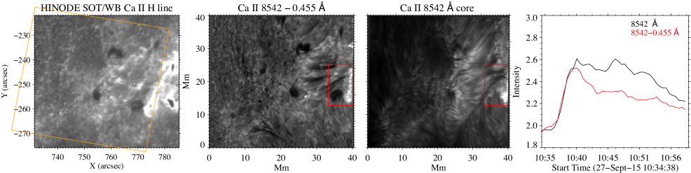
Figure 1: The Ca ii 8542 ${\AA}$ line wing and core images obtained with the CRISP instrument at 10:40:00 UT on 2015 September 27. A context image of the flare in the Ca ii H wide band obtained with the Solar Optical Telescope is shown on the left panel. The orange box indicates the flaring region observed with CRISP. The temporal evolution of the region averaged over the 20$\times$20 pixel² area on the flare ribbon is presented on the far right panel.

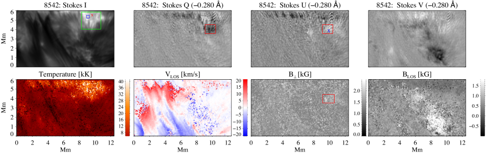
Figure 2: The top row shows the SST images in Ca 8542 Stokes $I$ at line core and $Q,~{}U$ and $V$ at $\mathrm{\Delta\lambda=-0.280~{}{\AA}}$ at 10:40:00 UT (flare peak) of the flaring region selected for inversions (marked with the red box in Figure 1). The NICOLE output showing the temperature, LOS velocity, and LOS magnetic field maps averaged over the interval between $\mathrm{log~{}\tau\approx-1.5~{}and-4}$, and perpendicular (with respect to the observer) magnetic field map in the interval between $\mathrm{log~{}\tau\approx-1~{}and-2.5}$, are presented in the bottom panels. The red and blue colors in the Dopplergrams represent positive Doppler velocities (downflows) and negative Doppler velocities (upflows), respectively. The ”x”, the blue, green and red boxes mark the selected representative pixels and regions at the flare ribbon that are discussed in the text.

The Ca ii infrared (IR) triplet lines are well suited for flare diagnostics due to its good sensitivity to physical parameters, including magnetic field, in the solar photosphere and chromosphere (Cauzzi et al., 2008; Pietarila et al., 2007; de la Cruz Rodríguez et al., 2012; Quintero Noda et al., 2016). Furthermore, calcium is singly ionized under typical chromospheric conditions, with negligible non-equilibrium and partial redistribution effects for the Ca ii IR lines (Uitenbroek, 1989; Wedemeyer-Böhm & Carlsson, 2011), making their modeling and interpretation of the observations more straightforward. Furthermore, the NLTE radiative transfer code NICOLE (Socas-Navarro et al., 2015) allows to perform the inversion of observed Ca ii 8542 Å (hereafter Ca 8542) Stokes profiles and the construction of semi-empirical model atmospheres. Such inversions have been successfully performed for spectropolarimetric Ca 8542 observations and 3D magnetohydrodynamical simulations of solar features in the umbra and penumbra of sunspots (de la Cruz Rodríguez et al., 2013; Henriques et al., 2017), granular-size magnetic elements (magnetic bubbles) in an active region, and magnetic flux tubes (de la Cruz Rodríguez et al., 2015a; Quintero Noda et al., 2017). Recently Kuridze et al. (2017) performed NICOLE inversions of high-resolution spectroscopic data in the Ca 8542 line and found that the temperature in the middle and upper chromosphere close to the flare peak is enhanced up to $\sim$6.5 - 20 kK between $\mathrm{log~{}\tau\sim-3.5~{}and-5.5}$, decreasing gradually to preflare temperatures of $\sim$5 - 10 kK approximately 15 minutes after the peak.

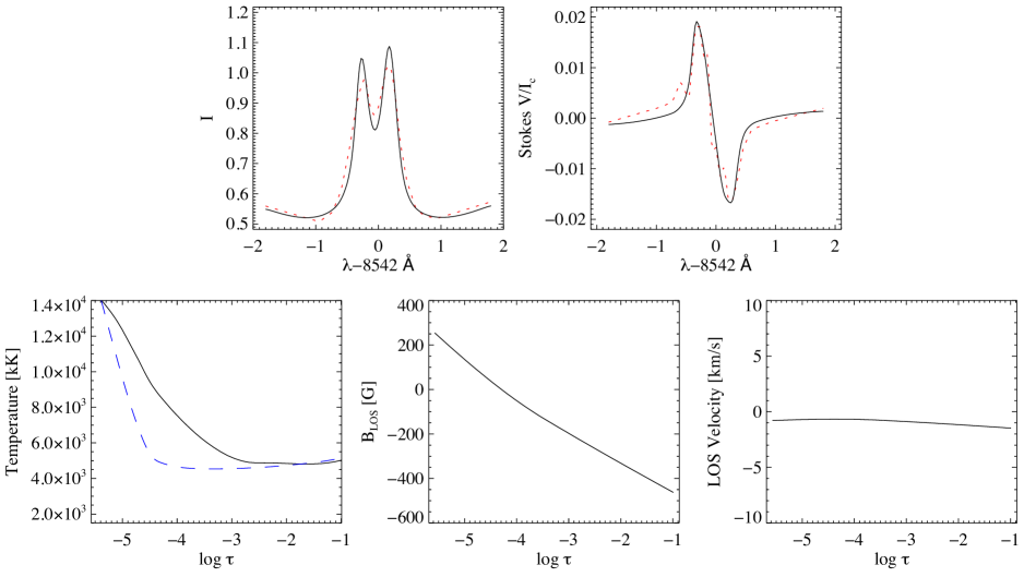
Figure 3: A representative example of the observed (red dotted) and best-fit synthetic (black) Ca 8542 line Stokes $I$ and $V$ profiles together with temperature, velocity and LOS magnetic field stratifications for the flaring pixel marked with the red ’x’ in Figure 2. The blue dashed line depicts the typical temperature stratification obtained from inversions for a non-flaring pixel located at around x=1, y=4 Mm in the selected region (Figure 2).

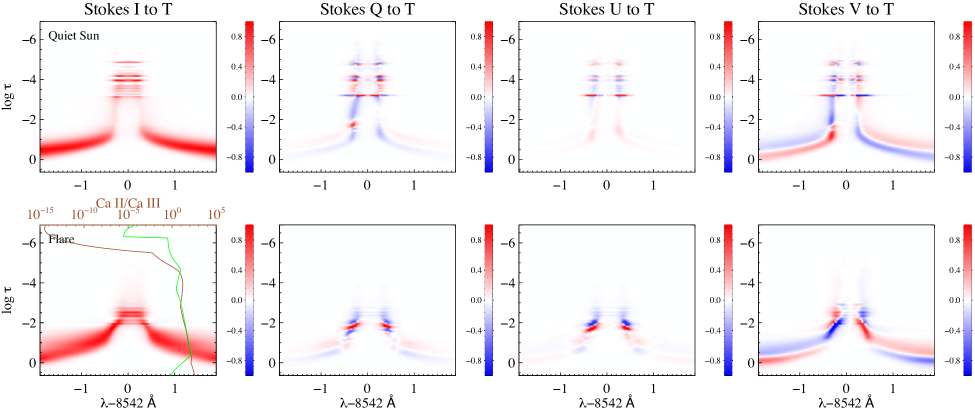
Figure 4: Two dimensional plots of the RFs (normalised to their maximum values) which show how given Stokes profiles respond to changes in the temperature for Ca 8542 line for the area covering the non-flaring, quiet Sun region (top row) and the flare ribbon (bottom row) at 10:40:00 UT. The ratio of the population densities of Ca ii and Ca iii as a function of height for QS (green line) and flare (brown line) models are overplotted in the bottom left panel.

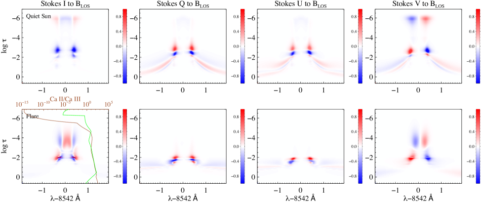
Figure 5: Two dimensional plots of the RFs which show how given Stokes profiles respond to changes in the LOS magnetic field for Ca 8542 line for the area covering the non-flaring, quiet Sun region (top row) and the flare ribbon (bottom row) at 10:40:00 UT. The ratio of the population densities of Ca ii and Ca iii as a function of height for QS (green line) and flare (brown line) models are overplotted in the bottom left panel.

Spectropolarimetric data of the flare in the Ca ii 8542 and He ii 10830 Å lines have been analyzed in several works (Penn & Kuhn, 1995; Sasso et al., 2011; Kleint & Judge, 2011; Kuckein et al., 2015a, b; Judge et al., 2014, 2015). Using photographic recordings of Stokes $I$ and $V$ profiles in the Ca ii H line, Martinez Pillet et al. (1990) derived a value of 820 ($\pm$40) G for B_LOS using the weak field approximation. Harvey (2012) studied the vector magnetic field in the Ca 8542 line and measured its LOS component for two flare kernels to be 415 and - 215 Gauss. Recently, Kleint (2017) detected the stepwise chromospheric LOS magnetic field changes obtained through spectropolarimetry of Ca 8542 during an X-class flare. The Stokes $Q$ and $U$ signals across the line profiles and the associated transverse component of the magnetic field are more difficult to observe, as the variation of $Q$ and $U$ is, in general, more complex with less polarimetric sensitivity than the Stokes $V$ profile and are more affected by instrumental smearing (Leone et al., 2017). Kleint (2012) detected linear polarization of up to 10% of the continuum level in the Ca 8542 line in the flare ribbons located over the sunspot with typical symmetric Zeeman signatures.

In this paper we analyze high-resolution imaging spectropolarimetric observations of an M-class solar flare in Ca 8542 line. We use NICOLE to invert the full Stokes profiles and construct models for the lower atmosphere of the flare event. Multiple inversions were performed for the observed region, covering flare ribbons and non-flaring areas at different times during the event. The constructed models are used to obtain diagnostic information on key plasma parameters which focus on temperature, velocity, and magnetic field stratifications in the upper photosphere and chromosphere during the flare. The chromospheric magnetic field was also evaluated using the weak-field approximation method.

2 Observations and data reduction

The observations were obtained between 10:34 and 10:59 UT on 2015 September 27 close to the West limb ($774^{\prime\prime}$, $-217^{\prime\prime}$, $\mu\approx$ 0.545) with the CRisp Imaging SpectroPolarimeter (CRISP; Scharmer, 2006; Scharmer et al., 2008) instrument, mounted on the Swedish 1-m Solar Telescope (SST; Scharmer et al., 2003) on La Palma. The observations comprised of imaging spectropolarimetry in Ca 8542 line. The data were reconstructed with Multi-Object Multi-Frame Blind Deconvolution (MOMFBD; Löfdahl, 2002; van Noort et al., 2005). We applied the CRISP data reduction pipeline as described in de la Cruz Rodríguez et al. (2015b) which includes small-scale seeing compensation for spectral scans as in Henriques (2012). Our FOV was $41\times 41$ Mm² with a spatial sampling was 0^′′.057 pixel^-1. The spatial resolution was close to the diffraction limit of the telescope at this wavelength (0^′′.18) for many images in the time-series. All profiles were normalized to the continuum of the quiet-Sun intensity by fitting the FTS atlas profile (Neckel, 1999) convolved with the CRISP instrumental profile.

The Ca 8542 line scan consisted of 21 line positions with an irregular step size. From line core these were: -1.75 Å to +1.75 Å ($\pm$1.75, $\pm$0.945, $\pm$0.735, $\pm$0.595, $\pm$0.455, $\pm$0.35, $\pm$0.28, $\pm$0.21, $\pm$0.14, $\pm$0.07, 0.0 Å). The cadence of the time series was 22.3 s. The transmission FWHM for Ca 8542 is 107.3 mÅ with a pre-filter FWHM of 9.3 Å. Throughout the analysis we made use of CRISPEX (Vissers & Rouppe van der Voort, 2012), a versatile widget-based tool for effective viewing and exploration of multi-dimensional imaging spectroscopy data.

The M1.9 flare was observed on active region NOAA 12423. The rise phase and flare peak were captured during the observations. Figure 1 shows a sample of the flare images in the Ca 8542 line core and wing positions. Unfortunately, our ground-based observations covered only $\sim 20\%$ of the flare ribbon. Context imaging of the full ribbon are provided by the Ca ii H wide band filtergrams obtained with the Solar Optical Telescope on board the HINODE satellite (Kosugi et al., 2007; Tsuneta et al., 2008) (see Figure 1). Lightcurves generated from the region located on the ribbon show the evolution of the emission in the line core and wing positions (right panel of Figure 1).

3 Inversions

Table 1: Number of nodes and input atmosphere models used during each cycle (Cy) of the inversion.

Physical parameter	Cy 1	Cy 2
Temperature	6 nodes	7 nodes
LOS Velocity	2 nodes	3 nodes
Microturbulence	1 node	1 node
$\mathrm{B_{z}}$	2 nodes	3 nodes
$\mathrm{B_{x}}$	2 nodes	3 nodes
$\mathrm{B_{y}}$	2 nodes	3 nodes
Macroturbulence	none	none
Input atmosphere	Fal-C	model from Cy 1

We used the NICOLE inversion code (Socas-Navarro et al., 2015) which has been parallelized to invert large field of view (one pixel at a time) and solves multi-level, NLTE radiative transfer problems (Socas-Navarro & Trujillo Bueno, 1997). The code iteratively perturbs physical parameters such as temperature, LOS velocity, magnetic field and microturbulence of an initial guess model atmosphere to find the best match with the observations (Socas-Navarro et al., 2000).

We used a five bound level plus continuum Ca 8542 model atom with complete angle and frequency redistribution, which is applicable to lines such as Ca 8542 (Shine & Linsky, 1974; Uitenbroek, 1989). The synthetic spectra were calculated for a wavelength grid of 145 datapoints in 0.025 Å steps, 6 times denser than the CRISP dataset. Stratification of the atmospheric parameters obtained by the inversions are given as a function of the logarithm of the optical depth-scale at 500 nm (hereafter $\mathrm{log~{}\tau}$).

To improve convergence, the inversions were performed in two cycles, expanding on the suggestion of Ruiz Cobo & del Toro Iniesta (1992). In the first cycle we use the FAL-C atmosphere (Fontenla et al., 1990) as an initial model. Table 1 summarizes the number of nodes and initial temperature models used in the two cycles.

We inverted a 300 $\times$ 160 pixel² area (12.3$\times$6.5 Mm²) covering the flare ribbons as well as some non-flaring regions (see left panels of Figure 1). The Stokes profiles were rebinned in $\mathrm{2\times 2}$ pixels to increase the signal to noise ratio. Although our time-series comprises of 46 spectral scans, we only choose the best scans in terms of spatial resolution which limits the total number of inverted scans to 8.

To investigate the sensitivity of the Ca 8542 line to changes of the atmospheric parameters at different heights in the lower solar atmosphere, we have also computed the numerical response function of the emergent profile using the different models obtained from inversions.

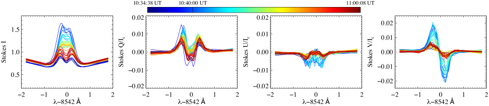
Figure 6: Temporal evolution of the observed Ca 8542 Stokes profiles averaged over the region outlined with the blue box in Figure 2 starting $6$ minutes before the flare peak (10:40:00 UT).

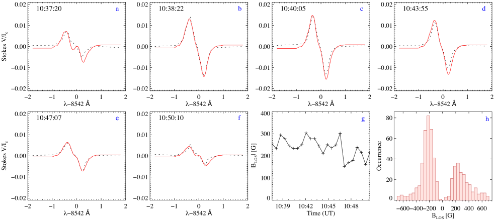
Figure 7: (a-f) Circular polarization profiles (black dashed lines) for the flare ribbon at different phases of the event for the region outlined with the blue box in Figure 2. WFA fits obtained from the derivative of Stokes $I$ are depicted as full red lines. (g) The LOS magnetic field used to fit the Stokes $V$ as a function of time is presented in panel (g). (h) A histogram of the LOS magnetic field, from the fitting of Stokes $V$ profiles using the WFA for individual pixels of the area marked with the green box in Figure 2 during the flare peak (at 10:40:00 UT).

4 Analysis and results

The top row of Figure 2 presents the Ca 8542 Stokes $I$ at line core and $Q,~{}U$ and $V$ monochromatic images at $\mathrm{\Delta\lambda=-0.280~{}{\AA}}$ at 10:40:00 UT (flare peak) of the region selected for inversions (marked with the red box in Figure 1). The images show that the enhancement of circular and linear polarization signals (Stokes $V$ and $Q~{}\&~{}U$, respectively) are co-spatial with the flare ribbons observed in intensity (Stokes $I$). The NICOLE output showing the temperature, LOS velocity, and LOS magnetic field maps integrated between $\mathrm{log~{}\tau\approx-1.5~{}and-4}$ and averaged over this range, and perpendicular ($B_{\bot}$ along LOS) magnetic field maps integrated and averaged between $\mathrm{log~{}\tau\approx-1~{}and-2.5}$, are presented in the bottom panels of Figure 2. A temperature map of the inverted region shows strong temperature enhancements for the ribbon. The LOS velocity map of the same region reveals weak upflows within the ribbon area and some strong downflows nearby where chromospheric fibrillar features are located (Figure 2). The inversion results for the perpendicular magnetic field map are very noisy and inconsistent throughout the FOV. However, these results trace the shape of a patch of strong (around 1 - 1.5 kG) perpendicular field along LOS for the part of the flare ribbon where linear polarization is strongest (area marked with a red box on Figure 2 and region immediately to the right displaying a wing-like shape). The LOS magnetic field map is less noisy and tracing magnetic field concentrations at the vicinity of a small sunspot located at the bottom right part of the FOV and at the flare ribbon (bottom right panel of Figure 2).

Figure 3 shows the observed Stokes profiles (red dotted lines) of the flaring pixel marked with red ’x’ in Figure 2 at the flare peak ($\sim$10:40:00 UT). The best-fit synthetic profiles obtained from the inversion are also shown as full black lines. The temperature, LOS magnetic field and velocity stratifications reproducing the synthetic profiles of this pixel are presented at the bottom panels of Figure 3. The Stokes $I$ profile is centrally reversed and shows excess emission in the red wing (red asymmetry) with a blueshifted line center (top left panel of Figure 3). The asymmetry appears to be due to the blueshifted line core of Stokes $I$ which in turn is a consequence of upflows (visible in our inversions in the bottom right panel of Figure 3) at the height of line core formation (Carlsson & Stein, 1997; Abbett & Hawley, 1999; Kuridze et al., 2015, 2016, 2017). The flare pixel has a higher chromospheric temperature at $\mathrm{log~{}\tau\sim-2.5~{}and-5.5}$ compared to the quiet Sun temperature profile which is overplotted as a blue dashed line at the bottom left panel of Figure 3. The Stokes $Q$ and $U$ profiles are very noisy which caused NICOLE to fail in the fitting of a perpendicular magnetic field stratification. The analysis of the line response functions shows that the inversions provide diagnostics for the LOS magnetic field in the layers between $\mathrm{log~{}\tau\sim-1~{}and-4.5}$ (see Figure 4 & 5). The absolute value of the LOS magnetic field in the lower atmosphere between $\mathrm{log~{}\tau\sim-1~{}and-4.5}$ decreases gradually with an almost linear trend from $\mathrm{|B_{LOS}|}$=450 G to $\sim$0 G (Figure 3).

It must be noted that the imaging spectropolarimetric data analysed in this work are limited by the acquisition time required for a spectral scan of line profiles. Recently, Felipe et al. (2018) investigated the impact of the time-dependent acquisition on the inversion of spectropolarimetric profiles of Ca 8542 line during umbral flashes. They showed that the inversion results could be unreliable at the development phase of the flash when the atmosphere is changing rapidly due to the time-dependent acquisition of line profiles. They have considered an extreme case where the line profiles are changing from absorption to emission during the scan. The flaring atmosphere can also change rapidly during the scanning time, especially at the impulsive phase of the flare which is characterised by very short dynamical timescale. However, temporal evolution of line profiles analysed in this work are not suggesting that they are changing significantly during the scan. Furthermore, lightcurves generated from the region located on the ribbon also indicates that flare has a much longer evolution timescale when compared to the acquisition time of the Ca 8542 line profiles ($\mathrm{\sim 15~{}s}$) (see right panel of Figure 1).

To investigate how sensitive the Ca 8542 line is to the different layers of the atmosphere (in $\mathrm{log~{}\tau}$ units) covered by the models, we need to examine the response function (RF), which measures the response of the emergent profiles to perturbations of the physical parameters. We compute the numerical RFs for the Stokes profiles for different atmospheric models obtained from NICOLE inversions. Figures 4 and 5 show 2 dimensional plots of the RFs of the given Stokes profiles to changes in the temperature and LOS magnetic field for the area covering the flare ribbon and for the non-flaring quiet Sun region. RFs to the temperature of the QS Ca 8542 Stokes profiles, covering a $\mathrm{\pm 1.75~{}{\AA}}$ spectral range from the line core, are expanded to $\mathrm{log~{}\tau\sim-1~{}and-5}$. However, Stokes $Q~{}\&~{}U$ have very small sensitivity to temperature in the outer wings beyond $\mathrm{\pm 1~{}{\AA}}$ from the line core (top panels of Figure 4). For the flare model RFs to temperature for the Stokes profiles have enhancements between $\mathrm{log~{}\tau\sim-1~{}and-3}$ with very small values between $\mathrm{log~{}\tau\sim-3~{}and-4.5}$.

The RFs to the LOS magnetic field of the QS model for the Ca 8542 Stokes profiles show responses up to $\mathrm{log~{}\tau\sim-6}$ with a strong peak between $\mathrm{log~{}\tau\sim-1.5~{}and\sim-3.5}$ (top panels of Figure 5). However, the peaks of the RFs to the LOS magnetic field of the flare models are located deeper in the atmosphere between $\mathrm{log~{}\tau\sim-1~{}and-2.5}$ (bottom panels of Figure 5). This indicates that the Ca 8542 Stokes profiles for the flare models are more sensitive to perturbations of the temperature and magnetic field in the deeper atmospheric layers than for QS atmosphere models. The RFs computed for multiple pixels from different regions consistently show similar changes in the sensitivity of Ca 8542 throughout the different QS and Flare models. To investigate the reason for this difference we analyzed the ionization level of Ca 8542 line in QS and flare models by computing the population densities of all Ca ii atomic levels over the population densities of Ca iii. The results for the QS (green line) and the flare (brown line) models are overplotted on the bottom left panels of Figure 4 and 5. The results show that the fraction of Ca ii to Ca iii decrease by about $\sim$100 times above $\mathrm{log~{}\tau\sim-4.5}$ when compared to the Ca ii/Ca iii in the QS atmosphere (Figure 4 & 5) indicating that Calcium is almost fully ionized to Ca iii above $\mathrm{log~{}\tau\sim-4.5}$. This can explain why the Ca 8542 Stokes profiles are less sensitive to the physical properties of the upper atmosphere during the flare.

Figure 6 displays the evolution of the Ca 8542 Stokes profiles located on the flare ribbon and averaged over the $\mathrm{\sim 0.35^{\prime\prime}\times 0.35^{\prime\prime}}$ area marked with the blue box in Figure 2. It shows that, as the flare initiates, the Stokes profiles of the area located on the ribbon increase in intensity, becoming strongest during the flare maximum and decreasing after the maximum. An enhancement of polarization signals could be related to the increase of Stokes $I$ amplitude. Stokes $V,~{}Q,~{}\&~{}U$ depend on the first and second derivatives of the intensity (Stokes $I$) in the weak field approximation (WFA) regime. We can apply the WFA here as the field strength is expected to be significantly lower than 2.5 kG and the Zeeman splitting is much smaller than the thermal width of the observed Ca 8542 line (de la Cruz Rodríguez et al., 2013). In this regime the Stokes profiles can be expressed as (Landi Degl’Innocenti & Landi Degl’Innocenti, 1977),

$$V(\lambda)=-4.67\times 10^{-13}g_{eff}\lambda_{0}^{2}B_{LOS}\frac{\partial I(\lambda)}{\partial\lambda},$$ (1)

$$\left[Q^{2}+U^{2}\right]^{1/2}=\left|-5.45\times 10^{-26}\bar{G}\lambda_{0}^{4}B^{2}_{\bot}\frac{\partial^{2}I(\lambda)}{\partial\lambda^{2}}\right|,$$ (2)

where $g_{eff}$ is the first order effective Landé factor, and $\lambda_{0}$ the central wavelength of the spectral line. $\bar{G}$ is a second order effective Landé factor related to $g_{eff}$ with

$$\bar{G}=g_{eff}^{2}-(g_{1}-g_{2})^{2}(16s-7d^{2}-4)/80,$$ (3)

where

$$s=J_{1}(J_{1}+1)+J_{2}(J_{2}+1),~{}~{}d=J_{1}(J_{1}+1)-J_{2}(J_{2}+1)$$

for the angular momentum $J_{1}$ and $J_{2}$ of the involved energy levels with Landé factors $g_{1}$ and $g_{2}$ (Landi Degl’Innocenti & Landi Degl’Innocenti, 1977). For Ca 8542 $g_{eff}$=1.1 and $\bar{G}$ =1.21. We note that the units for the wavelength and magnetic field are Å and Gauss, respectively.

Figure 7 (panels a - f) shows average Stokes $V$ profiles for the region outlined with the blue box in Figure 2 during the different phases of the flare together with the WFA fits obtained from the derivative of Stokes $I$ (overplotted as full red lines). The temporal evolution of the LOS magnetic field ($|B_{LOS}|$) used to fit the Stokes $V$ profiles at different times is presented in panel (g) of Figure 7. It shows that the average LOS magnetic field obtained with the WFA is around 250 $\pm$ 50 G until $\sim$10:47 UT, decreasing later down to 180 $\pm$ 30 G. Increased gradients in Stokes $I$, as those observed in the flare, lead to increased polarization signals and this is described in the WFA (Equations 1 & 2). Gradients of Stokes $I$ with respect to wavelength then certainly contribute to the observed enhanced amplitude of polarization signals (as in de la Cruz Rodríguez et al. 2012, Quintero Noda et al. 2017). However, such increases did not lead to WFA reproducing the flaring profiles without an increase in magnetic field. The increase in magnetic field could be related to the change of sensitivity of Ca 8542 in the chromosphere during the flare to lower layers where the field is expected to be stronger. As the atmosphere relaxes after the flare peak, the line becomes more sensitive to the higher levels of the atmosphere (Figure 4 & 5) where the magnetic field is expected to be weaker. A histogram of the LOS magnetic field computed with the fitting of Stokes $V$ using the WFA for individual pixels of the area marked with the green boxes in Figure 2 during the flare peak, is presented in panel (h) of Figure 7 showing median absolute values of 220$\pm$70 G.

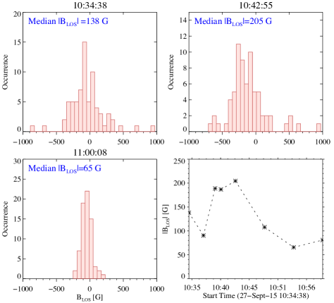
Figure 8: Histograms of $|B_{LOS}|$ computed from the semi-empirical models obtained from the inversions before, during and after the flare peak for the pixels of the area delimited with the green box in Figure 2 (after filtering for quality of fit). $|B_{LOS}|$ is averaged over optical depths ranging from $\mathrm{log~{}\tau\sim-1.5~{}to-4.5}$. Medians of $|B_{LOS}|$ for the same area obtained at 8 different points in time are presented in the bottom right panel.

Figure 8 shows the histograms of $|B_{LOS}|$ computed from the inversions before, during and after the flare peak for individual pixels of the area marked with the green box in Figure 2. $|B_{LOS}|$ is averaged over optical depths $\mathrm{log~{}\tau\sim-1.5~{}to-4.5}$. Models obtained at 8 different points in time were used to compute the median of $|B_{LOS}|$ for the same area. This temporal evolution is presented at the bottom right panel of Figure 8. It shows that 6 minutes before the flare peak the median of the integrated $|B_{LOS}|$ for the region marked with the green box in Figure 2 is around 138 G, increasing to 205 G at the flare peak (bottom right panel of Figure 8). After 10:47 UT $|B_{LOS}|$ decreases gradually to $\sim$70 G. We note that the models of the pixels with a low quality of fit were ignored and are not included in the histogram plots. The inverted LOS magnetic field evolution close to the flare peak, between 10:38 and 10:45 UT, is consistent with that of the $B_{LOS}$ evolution obtained with the WFA (shown in panel (g) of Figure 7), in that they show similar values and a decrease post 10:45 UT.

Compared with the LOS component, it is more challenging to compute the perpendicular component of the magnetic field along LOS with the WFA fitting as it is related to the total linear polarization, which depends on the second derivative of Stokes $I$ with respect to wavelength (Equation 2). Unfortunately, the observed Stokes $Q~{}\&~{}U$ can not be fitted reliably with the second derivative of Stokes $I$ under the WFA limit (Equation 2). To improve the quality of the signal we identified the area of the flare ribbon with the strongest amplitude in Stokes $Q~{}\&~{}U$ (red box on Figure 2), and computed averaged profiles over that $0.23^{\prime\prime}\times 0.23^{\prime\prime}$ area, followed by a NICOLE inversion. The representative example of Stokes profiles with the best-fit synthetic profiles obtained from the inversion for the pixel marked with the blue ’x’ in the red box on Figure 2 are presented on Figure 9. Temperature, LOS, and perpendicular magnetic field stratifications are shown on the bottom panels of Figure 9. The analysis of the response functions to the $B_{LOS}$ of Ca 8542 during the flare shows that inversions can provide diagnostics in the layers between $\mathrm{log~{}\tau\sim-1~{}and-2.5}$, with very small sensitivity between $\mathrm{log~{}\tau\sim-2.5~{}and-4}$ for Stokes $Q~{}\&~{}U$, and $\mathrm{log~{}\tau\sim-1~{}and-4}$ for Stokes $V$. $|B_{LOS}|$ in the atmosphere between $\mathrm{log~{}\tau\sim-1~{}and-4}$ is about $\sim$400-200 G whereas the $B_{\bot}$ in the atmosphere between $\mathrm{log~{}\tau\sim-1~{}and-2.5}$ is about 1.4 KG.

Despite the improved polarization signals, the total linear polarization ($\sqrt{Q^{2}+U^{2}}$) still can not be reliably fitted with the second derivative of Stokes $I$ under the WFA limit (Equation 2). Applying the WFA to the synthetic, best-fit profiles obtained from the inversion, led to a resulting total linear polarizatio that does not completely trace with the synthetic one (bottom left panel of Figure 9), however the resulting perpendicular component of the magnetic field is around 1300 G which is very close to the values obtained from the inversion (bottom third panel of Figure 9).

5 Discussion and conclusions

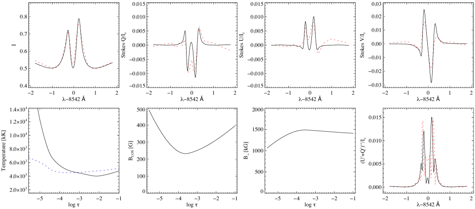
Figure 9: A typical set of Stokes profiles with corresponding well fitting synthetic profiles obtained from the inversion of a pixel from within the red box in Figure 2 averaged over that $0.23^{\prime\prime}\times 0.23^{\prime\prime}$ area, selected due to Stokes $Q$ and $U$ being successfully fitted. Temperature, LOS, and perpendicular magnetic field stratifications are shown in the bottom panels. The bottom right panel shows the synthetic, total linear polarization, $\sqrt{Q^{2}+U^{2}}$ (full black lines) and WFA fit (red dotted line) obtained from the second derivative of synthetic Stokes $I$.

We studied an M1.9 class solar flare using high-resolution full-Stokes imaging spectropolarimetric observations in the Ca ii 8542 Å  line. We used the non-LTE code NICOLE to construct semi-empirical models of the lower flaring atmosphere and investigate the temperature structure and magnetic field of the flare. Our analysis shows that the most intensively heated layers in the flaring lower atmosphere are the middle and upper chromosphere between optical depths $\mathrm{log~{}\tau\sim-2.5~{}and-5}$, with temperatures between $\sim$5 and 13 kK (Figure 2 and 3). In the photosphere, below $\mathrm{log~{}\tau\sim-2.5}$, there is no significant difference in the temperature stratification between quiescent and flaring atmospheres (Figure 3). This agrees with the previous results obtained by Kuridze et al. (2017) showing that during the C8.3 flare the atmosphere remained unchanged below $\mathrm{log~{}\tau\sim-2.5}$.

Our analysis shows that during flare maximum, the polarization signals of the ribbon in the chromosphere become stronger compared to its surroundings. To investigate if this relates to a change in the line formation height, we computed numerical RFs for the different semi-empirical models. The comparison of the RFs to perturbations in temperature and longitudinal magnetic field, between flaring and non-flaring atmospheres, shows that in the flaring atmosphere the Ca 8542 line is more sensitive to the lower layers than in the quiet Sun. This suggests that the formation of the line in the flaring atmosphere occurs in the deeper layers where the magnetic field is expected to be stronger which may result in the enhanced polarization signals. This analysis also indicates that the rapid flare heating of the chromosphere, significantly changes the balance between the population densities of the energy states in the Calcium atom and, most importantly, the fraction between Ca ii and Ca iii (Figure 4 $\&$ 5). The latter decreases by a factor of 100 above $\mathrm{log~{}\tau\sim-4.5}$ when compared to Ca ii/Ca iii in the QS atmosphere indicating that Ca ii is almost fully ionized to Ca iii above $\mathrm{log~{}\tau\sim-4.5}$. This can explain why the Ca ii Stokes profiles are less sensitive in the higher layers of the atmosphere during the flare (Figure 4 $\&$ 5). This is in agreement with Kerr et al. (2016) who show that, in dynamic flare models, the Ca ii becomes fully ionized above $\sim$600 km due to intense heating.

The averaged LOS magnetic field of the flare ribbon, as obtained from inversions over the range of $\mathrm{log~{}\tau\sim-1~{}to-4.5}$, is estimated as 150 G 6 minutes before flare maximum, increasing to $\sim$200 G at the flare peak, and decreasing to $\sim$65 G approximately 7 minutes after the peak (Figure 8). The chromospheric magnetic field was also determined using the WFA, which led to a very similar value of 220$\pm$70 G for the flare peak. The WFA approach also led to a post-flare decrease, although this was less pronounced compared to the inversion outputs ($\sim$170 $\pm$ 30 G approximately 6 minutes after the peak).

We note that for most pixels in the detailed analysis area (green box in Figure 2), there are very good matches between Stokes $V$ and $\partial I/\partial\lambda$ suggesting that the increase of Stokes $I$ amplitude is the main reason for the enhanced amplitude of polarization signals during the flare.

Estimating the transverse/perpendicular component of the magnetic field is extremely challenging as the linear polarization has low sensitivity for weak fields and the profiles obtained are usually noisier than those of circular polarization. Our inversions have led to good fits in a patch of strong $\mathrm{\sim 1-1.5}$ kG (fitted) perpendicular field, for the portion of the flare ribbon where linear polarization is the strongest (areas marked with red boxes on Figure 2). This is an unusually strong magnetic field for the chromosphere. We also applied the WFA fitting to the synthetic total linear polarization profiles obtained from the inversions and were able to reproduce the observed linear polarization profiles (Figure 9). The resulting perpendicular (with respect to the LOS) component of the magnetic field inside the area marked with the red box on Figure 2 is around 1300 G which is very close to the value obtained from inversions (bottom third panel of Figure 9).

LOS magnetic fields of the order of kG for chromospheric flare ribbons have been reported in previous studies. For example, Martinez Pillet et al. (1990) derived a value for B_LOS of 820 ($\pm$40) G with Stokes $I$ and $V$ profiles from the Ca ii H line and the WFA. Harvey (2012) evaluated B_LOS for a flare emission kernel to be 415 G using the Ca ii 8542 Å line, also with the WFA. Penn & Kuhn (1995) used the 10830 Å He i line and found mean B_LOS of about 735 G during the decay phase of the flare kernel. However, to our knowledge, perpendicular components of the magnetic field with respect to the observer of the order of kG have never been observed in the flaring chromosphere. Yet, if the perpendicular magnetic field with respect to the surface of the Sun close to the disk center can reach up to kG level in the flaring chromosphere then, away from the disk center, this field can be observed as the strong perpendicular field with respect to the LOS. The observed region analyzed in this work is located away from the disk center (with $\mu\approx$ 0.545) and hence the magnetic field of the flaring loops located in this particular area of flare ribbon (red box on Figure 2) can be oriented perpendicularly with respect to the observer. This can be a reason of an observed enhanced amplitudes of linear polarization signal and strong perpendicular component of the magnetic field.

Our analysis shows that the increased amplitude of the Stokes profiles including polarization signals related to flare energy release in the lower solar atmosphere allow reliable measurement of the chromospheric magnetic field. Good agreement between the measured magnetic field using multi-node inversions in NLTE and WFA fitting, strongly suggests that both methods can be successfully applied to the flaring chromosphere.

References

- Abbett & Hawley (1999) Abbett, W. P., & Hawley, S. L. 1999, ApJ, 521, 906
- Carlsson & Stein (1997) Carlsson, M., & Stein, R. F. 1997, ApJ, 481, 500
- Cauzzi et al. (2008) Cauzzi, G., Reardon, K. P., Uitenbroek, H., et al. 2008, A&A, 480, 515
- de la Cruz Rodríguez et al. (2015a) de la Cruz Rodríguez, J., Hansteen, V., Bellot-Rubio, L., & Ortiz, A. 2015a, ApJ, 810, 145
- de la Cruz Rodríguez et al. (2015b) de la Cruz Rodríguez, J., Löfdahl, M. G., Sütterlin, P., Hillberg, T., & Rouppe van der Voort, L. 2015b, A&A, 573, A40
- de la Cruz Rodríguez et al. (2013) de la Cruz Rodríguez, J., Rouppe van der Voort, L., Socas-Navarro, H., & van Noort, M. 2013, A&A, 556, A115
- de la Cruz Rodríguez et al. (2012) de la Cruz Rodríguez, J., Socas-Navarro, H., Carlsson, M., & Leenaarts, J. 2012, A&A, 543, A34
- Felipe et al. (2018) Felipe, T., Socas-Navarro, H., & Przybylski, D. 2018, ArXiv e-prints, arXiv:1802.05028
- Fletcher et al. (2011) Fletcher, L., Dennis, B. R., Hudson, H. S., et al. 2011, Space Sci. Rev., 159, 19
- Fontenla et al. (1990) Fontenla, J. M., Avrett, E. H., & Loeser, R. 1990, ApJ, 355, 700
- Harvey (2012) Harvey, J. W. 2012, Sol. Phys., 280, 69
- Henriques (2012) Henriques, V. M. J. 2012, A&A, 548, A114
- Henriques et al. (2017) Henriques, V. M. J., Mathioudakis, M., Socas-Navarro, H., & de la Cruz Rodríguez, J. 2017, ApJ, 845, 102
- Hirayama (1974) Hirayama, T. 1974, Sol. Phys., 34, 323
- Judge et al. (2014) Judge, P. G., Kleint, L., Donea, A., Sainz Dalda, A., & Fletcher, L. 2014, ApJ, 796, 85
- Judge et al. (2015) Judge, P. G., Kleint, L., & Sainz Dalda, A. 2015, ApJ, 814, 100
- Kerr et al. (2016) Kerr, G. S., Fletcher, L., Russell, A. J. B., & Allred, J. C. 2016, ApJ, 827, 101
- Kleint (2012) Kleint, L. 2012, ApJ, 748, 138
- Kleint (2017) —. 2017, ApJ, 834, 26
- Kleint & Judge (2011) Kleint, L., & Judge, P. 2011, in Bulletin of the American Astronomical Society, Vol. 43, AAS/Solar Physics Division Abstracts #42, 3.08
- Kosugi et al. (2007) Kosugi, T., Matsuzaki, K., Sakao, T., et al. 2007, Sol. Phys., 243, 3
- Kuckein et al. (2015a) Kuckein, C., Collados, M., & Manso Sainz, R. 2015a, ApJ, 799, L25
- Kuckein et al. (2015b) Kuckein, C., Collados, M., Sainz, R. M., & Ramos, A. A. 2015b, in IAU Symposium, Vol. 305, Polarimetry, ed. K. N. Nagendra, S. Bagnulo, R. Centeno, & M. Jesús Martínez González, 73–78
- Kuridze et al. (2017) Kuridze, D., Henriques, V., Mathioudakis, M., et al. 2017, ApJ, 846, 9
- Kuridze et al. (2015) Kuridze, D., Mathioudakis, M., Simões, P. J. A., et al. 2015, ApJ, 813, 125
- Kuridze et al. (2016) Kuridze, D., Mathioudakis, M., Christian, D. J., et al. 2016, ApJ, 832, 147
- Landi Degl’Innocenti & Landi Degl’Innocenti (1977) Landi Degl’Innocenti, E., & Landi Degl’Innocenti, M. 1977, A&A, 56, 111
- Leone et al. (2017) Leone, F., Scalia, C., Gangi, M., et al. 2017, ApJ, 848, 107
- Löfdahl (2002) Löfdahl, M. G. 2002, in Presented at the Society of Photo-Optical Instrumentation Engineers (SPIE) Conference, Vol. 4792, Society of Photo-Optical Instrumentation Engineers (SPIE) Conference Series, ed. P. J. Bones, M. A. Fiddy, & R. P. Millane, 146–155
- Martinez Pillet et al. (1990) Martinez Pillet, V., Garcia Lopez, R. J., del Toro Iniesta, J. C., et al. 1990, ApJ, 361, L81
- Neckel (1999) Neckel, H. 1999, Sol. Phys., 184, 421
- Penn & Kuhn (1995) Penn, M. J., & Kuhn, J. R. 1995, ApJ, 441, L51
- Pietarila et al. (2007) Pietarila, A., Socas-Navarro, H., & Bogdan, T. 2007, ApJ, 663, 1386
- Quintero Noda et al. (2016) Quintero Noda, C., Shimizu, T., de la Cruz Rodríguez, J., et al. 2016, MNRAS, 459, 3363
- Quintero Noda et al. (2017) Quintero Noda, C., Kato, Y., Katsukawa, Y., et al. 2017, MNRAS, 472, 727
- Ruiz Cobo & del Toro Iniesta (1992) Ruiz Cobo, B., & del Toro Iniesta, J. C. 1992, ApJ, 398, 375
- Sasso et al. (2011) Sasso, C., Lagg, A., & Solanki, S. K. 2011, A&A, 526, A42
- Scharmer (2006) Scharmer, G. B. 2006, A&A, 447, 1111
- Scharmer et al. (2003) Scharmer, G. B., Bjelksjo, K., Korhonen, T. K., Lindberg, B., & Petterson, B. 2003, in Society of Photo-Optical Instrumentation Engineers (SPIE) Conference Series, Vol. 4853, Innovative Telescopes and Instrumentation for Solar Astrophysics, ed. S. L. Keil & S. V. Avakyan, 341–350
- Scharmer et al. (2008) Scharmer, G. B., Narayan, G., Hillberg, T., et al. 2008, ApJ, 689, L69
- Shine & Linsky (1974) Shine, R. A., & Linsky, J. L. 1974, Sol. Phys., 39, 49
- Socas-Navarro et al. (2015) Socas-Navarro, H., de la Cruz Rodríguez, J., Asensio Ramos, A., Trujillo Bueno, J., & Ruiz Cobo, B. 2015, A&A, 577, A7
- Socas-Navarro & Trujillo Bueno (1997) Socas-Navarro, H., & Trujillo Bueno, J. 1997, ApJ, 490, 383
- Socas-Navarro et al. (2000) Socas-Navarro, H., Trujillo Bueno, J., & Ruiz Cobo, B. 2000, ApJ, 530, 977
- Tsuneta et al. (2008) Tsuneta, S., Ichimoto, K., Katsukawa, Y., et al. 2008, Sol. Phys., 249, 167
- Uitenbroek (1989) Uitenbroek, H. 1989, A&A, 213, 360
- van Noort et al. (2005) van Noort, M., Rouppe van der Voort, L., & Löfdahl, M. G. 2005, Sol. Phys., 228, 191
- Vissers & Rouppe van der Voort (2012) Vissers, G., & Rouppe van der Voort, L. 2012, ApJ, 750, 22
- Wedemeyer-Böhm & Carlsson (2011) Wedemeyer-Böhm, S., & Carlsson, M. 2011, A&A, 528, A1