Bell correlations at finite temperature
Abstract
We show that spin systems with infinite-range interactions can violate at thermal equilibrium a multipartite Bell inequality, up to a finite critical temperature . Our framework can be applied to a wide class of spin systems and Bell inequalities, to study whether nonlocality occurs naturally in quantum many-body systems close to the ground state. Moreover, we also show that the low-energy spectrum of the Bell operator associated to such systems can be well approximated by the one of a quantum harmonic oscillator, and that spin-squeezed states are optimal in displaying Bell correlations for such Bell inequalities.
1 Introduction
One of the key features of quantum physics, which challenges our every-day intuition, is the existence of nonlocal correlations [1]: Local measurements on a quantum system may lead to correlations whose nature departs entirely from the local hidden variable model (LHVM) paradigm, meaning that such correlations cannot be simulated locally by deterministic strategies, even if assisted by shared randomness [2].
Since Bell showed that quantum mechanics can produce correlations that do not admit a LHVM description [1], nonlocal correlations have had a fundamental interest per sé. Much work has been devoted to understand and characterize them (see [3] for a review). Moreover, Bell correlations constitute a resource that enables novel device-independent (DI) quantum information processing (QIP) tasks (such as DI quantum key distribution [4, 5], DI randomness amplification/expansion [6, 7] or DI self-testing [8, 9, 10]), thus providing an extra layer of security in QIP protocols, allowing to reduce their assumptions to a minimum level.
Bell correlations are strongly intertwined with entanglement, perhaps the most significant quantum phenomenon [11]. However, it is well known that entanglement and Bell correlations are inequivalent both in the bipartite [12] and in the multipartite [13, 14, 15] cases: Bell correlations are strictly stronger as they can only arise from entangled states, while the converse is not true in general (see e.g. [16]).
In the many-body regime, entanglement has proven to be key to the understanding of a plethora of physical phenomena [17]. Intensive studies of entanglement have elucidated its important role in modern physics’ central topics such as quantum phase transitions [18], superconductivity at high temperature [19], the holographic principle [20] or quantum chemistry reactions [21, 22]. Furtermore, entanglement lies at the heart of the tensor network ansatz [23], and could even be relevant to the understanding of quantum machine learning models [24].
However, the role played by nonlocal correlations in many-body physics is not so clear yet. Their complex characterization (see [25]), which is known to be NP-hard even in the bipartite case [26], has posed a barrier to the study of multipartite scenarios. For this reason, the implications of nonlocal correlations in systems consisting of a very large number of parties has been mostly lacking, despite remarkable results have been obtained throughout the years [27, 28, 29, 30, 31, 32, 33, 34, 35, 36, 37]. Interestingly, recent theoretical advances developed in the context of few-body Bell inequalities [38, 39, 40, 41, 42, 43, 44, 45, 46] have allowed for simple ways to detect these correlations in many-body systems. On the one hand, it has been shown that many-body observables such as the energy of the system could signal the presence of Bell correlations in the system [42]. On the other hand, routinely measured experimental quantities such as total spin components and higher moments thereof [47, 48], have been shown to be sufficient to formulate Bell correlation witnesses that can detect nonlocality in many-body systems [38, 39, 40, 41]. With these tools, such correlations have been observed experimentally in a Bose-Einstein Condensate of atoms [49] and in a thermal ensemble of atoms [50].
In this work, we study whether Bell-nonlocal states (i.e., quantum states with the potential to produce Bell correlations if one were to perform a proper loophole-free Bell test on them) appear naturally in the low-energy spectrum of physically relevant Hamiltonians. As shown in [38, 39, 42], partial answers to this question are given, by noticing that the ground state of some spin Hamiltonians can violate a Bell inequality. However, conclusions for more experimentally relevant situations, such as non-zero temperature or systems with infinite-range interactions are still missing.
Here, we show that a many-body spin system at finite temperature can violate a Bell inequality and we quantify this violation. We also show that the low-energy part of the spectrum of the Bell operator corresponding to the optimal measurements of the Bell inequality can be well approximated by a quantum harmonic oscillator, enabling a connection to squeezed states. We observe a critical temperature above which nonlocality cannot be detected with our inequality, raising the question of whether this phenomenon can be observed in other systems and with other inequalities. This could allow to observe Bell-nonlocal states appearing naturally in solid-state systems cooled below some transition temperature.
2 Spin model
We consider a system of spins, described by an Ising model with infinite-range interactions. With denoting the vector of spin operators for the -th particle, the Hamiltonian of the system is
| (1) |
where is the external magnetic field and the strength of the spin-spin coupling. Since Eq. (1) has a preferred direction, we can assume, without loss of generality, that . The case of interest for our study corresponds to and , which we shall assume throughout the rest of the paper. Since , the spin-spin interaction is antiferromagnetic.
Using the definition of collective spin operator , given by
| (2) |
we rewrite Eq. (1) as
| (3) |
Here, and in the following, we shall not drop the constant term in the Hamiltonian, as it will be important later on.
Hamiltonians of this form, where interactions are of infinite range, are routinely realized in a number of experiments on many-body systems. Examples include Bose-Einstein condensates [51, 52, 53], atomic ensembles in optical cavities [54], and ion crystals [55, 56].
We are interested in the limit , for which the energy of (cf. Eq. (3)) is minimized when the collective spin has the maximum length and pointing direction along (since ). To approximate the low-energy spectrum of , we perform the Holstein-Primakoff transformation, which maps the collective spin to a bosonic mode [57]
| (4a) | ||||
| (4b) | ||||
| (4c) | ||||
with , being respectively the bosonic creation and annihilation operators acting on the Fock space, and satisfying the canonical commutation relation . Because we are interested in the low-energy excitations above the ground state, i.e. the case where and , we further approximate in Eqs. (4b) and (4c). Note that implies we are considering a small number of bosonic excitations. These bosonic modes arise from the Holstein-Primakoff transformation and can be seen as “fictitious” bosonic modes. As it can be seen from (4a), they are excitations of the spin system that reduce . This allows us to approximate Eq. (3) with the expression
| (5) |
This Hamiltonian is diagonalized by performing the Bogoliubov (squeezing) transformation [58, 59]
| (6a) | ||||
| (6b) | ||||
with and defined as
| (7) |
and , being newly defined bosonic creation and annihilation operators satisfying the canonical commutation relation . With Eqs. (6) we express Eq. (2) in the diagonal form
| (8) |
In the limit the last term of Eq. (2) tends to , leaving us with the Hamiltonian , defined as
| (9) |
Note that the Hamiltonian in Eq. (2) describes a quantum harmonic oscillator of frequency
| (10) |
and its energy spectrum is given by
| (11) |
where and . Eq. (2) shows us that the ground state of is approximated by the ground state of , which has and (remember ).
It is important to realize that the spectrum in Eq. (2) has two characteristic spacings: In the limit , one is , and the other is . This shows that for large , the low-energy part of the spectrum is dominated by excitations of and different . Note that, for large values of , scales as , whereas remains approximately constant. This implies that for sufficiently large values of , the latter constant becomes effectively arbitrarily small, and therefore many levels of become accessible.
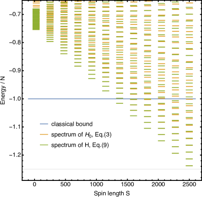
For a graphical comparison, we plot in Fig. 1 the spectrum of the Hamiltonian Eq. (1), and of its approximation Eq. (2), for , , , and some values of (the reason for this specific choice of parameters will be clear in Sec. 4). We can see that low-energy excitations of the two models are very similar. As expected, energy levels for and are very well described by the Holstein-Primakoff approximation. Note also that this match improves as .
It should be noted that the state yielding the ground energy of the family of Hamiltonians considered is spin-squeezed, as these Hamiltonians are diagonalized via the spin-squeezing transformation (cf. Eq. (6)). In Sec. 4 we shall see that the Hamiltonians we consider can be mapped into Bell inequalities. For this reason we conclude that spin-squeezed states are optimal for violating such inequalities, in the sense that they asymptotically (as goes to infinity) give the maximal quantum violation [39].
To describe the system at finite-temperature, it is crucial to keep track of the degeneracy of the energy levels, originating from the multiplicities of the blocks with given (see e.g. [60, 61]). This is 1 if and otherwise it is given by
| (12) |
The derivation of follows from representation theory results such as the Shur-Weyl duality. We refer the interested reader to [62, 63, 64] for their derivations in quantum information and mathematical contexts.
In the following we will consider two different regimes. The first one is the low temperature regime, where and . In this case we can perform the following approximation: For and , the leading term in is given by the factor . The second regime of interest corresponds to , and therefore the previous approximation cannot be done. We will discuss how to treat this case in detail in Sections 3 and 5.
3 Partition function
In this section we introduce the standard tools of statistical mechanics that are needed to describe a system at finite-temperature. In particular, expectation values of interest are computed from the partition function of the considered statistical ensemble. As we consider a system in thermal equilibrium at temperature and with fixed number of atoms , we are in the canonical ensemble. The canonical partition function for the system described by Eq. (2) is given by
| (13) |
with the degeneracy (independent of ) of the energy level , and is the inverse temperature. Performing the sum over leaves us with
| (14) |
The argument of the summation is a complicated expression, and for this reason there is no general analytical solution for . As we will be interested in two specific temperature regimes, we approximate the sum by looking at which terms are relevant.
In the low temperature regime, , the sum over will be dominated by values of . This can easily be seen e.g. by plotting the terms of the sum in (14) as a function of . Then one sees that only the terms that are close to contribute. This observation allows us to set , which becomes independent of . Therefore, the denominator of Eq. (14) can be taken outside the sum. Since in this case the approximation holds, we can find an analytical expression for the summation over :
| (15) | ||||
| (16) |
To summarize, in the low-temperature regime the canonical partition function can be approximated by
| (17) |
The second temperature regime of our interest is the one for which , for a reason that will be clear in the following. At this temperature, and for the parameters and introduced later, we observe that the terms in the sum of Eq. (14) are dominant for . In this situation, we cannot provide an accurate and simple approximation to , and therefore we adopt a different approach. By observing that in the limit the terms in the summation of Eq. (14) follow a Gaussian distribution with mean , we approximate them in this way. Finally, the sum is replaced by an integral which can be easily computed for a Gaussian. The resulting (approximated) partition function is an analytical expression too complicated to be written here (see Appendix), and therefore we will only present some results computed from it.
The crucial quantity of our interest will be the total energy of the system at finite temperature, which is defined as
| (18) |
In the regime and we find
| (19) |
For the parameters of our interest, and , this becomes
| (20) |
For these specific parameters, we find in the regime and the simple expression
| (21) |
4 Bell inequality
In this section we introduce the class of inequalities with which we consider to detect Bell correlations at finite temperature. We note that our scenario of interest is not the one in which a loophole-free Bell test is performed, but rather, in which one certifies the presence of a Bell-nonlocal state; i.e., a quantum state capable to produce Bell correlations if a proper loophole-free Bell test were performed upon it. We also recall the mapping between multipartite Bell inequalities and quantum Hamiltonians. In particular, we show how the Bell operator associated to the inequalities of our interest is related to the Hamiltonian in Eq. (1).
We consider the simplest multipartite Bell experiment, in which spatially separated observers labelled from to hold their shares of a quantum system and have at their disposal two dichotomic measurements each. The measurements are labelled or , and they can yield outcomes . We denote the -th measurement performed on the -th party . We are interested in Bell inequalities that involve only symmetric one- and two-body correlators, as they are the simplest to be accessed experimentally. These correlators are defined as
| (22) | ||||
| (23) |
and they yield Bell inequalities of the following form [38, 39]:
| (24) |
where is the so-called classical bound and , are real parameters.
To illustrate our framework, we shall focus on the multipartite Bell inequality considered in [38],
| (25) |
even if our method can be straightforwardly adapted to any other inequality of the form of Eq. (24).
Because Ineq. (25) has two settings and two outcomes, it can be minimized with traceless real qubit measurements [65]. For this reason, without loss of generality, it is enough to consider and . As shown in [39], only the angle between and matters, and therefore it is also possible to choose , which allows us to transform the Bell inequality (25) into the Bell operator
| (26) |
where stands for ; i.e., being a positive semidefinite operator. Moreover, in the limit of it was found [39] that the optimal measurement angle is . This gives, with the definition , the Bell operator
| (27) |
Since for all local states, observing witnesses nonlocality.
At this point, we can motivate our choice of the parameters and for Eq. (1). This particular case is of special interest as it results in a spin model whose Hamiltonian is identical to the Bell operator Eq. (4).
Now the idea is simple: since the specific Bell inequality and spin Hamiltonian we considered can be mapped one into the other, the energy of our spin system can be identified to the expectation value of the Bell operator, i.e. . For low enough temperatures the energy of the system will be lower than the classical bound, implying the presence of Bell correlations.
5 Nonlocality versus temperature
We now investigate the dependence of on the temperature . We plot in Fig. 2 the mean energy (cf. Eq. (18)) per particle as a function of , for . This modest number of particles allows us to compute numerically the exact partition function Eq. (14), and from it the mean energy per particle (orange line in Fig. 2). Comparing this latter to the classical bound of the Bell operator Eq. (4) normalized per particle, (blue line in Fig. 2), shows a violation of the inequality up to a temperature of (see the intersection between the orange and the blue line in Fig. 2).
In the limit , we are interested in finding the critical temperature above which nonlocality is not detected by the inequality we considered. Naively, from the low temperature approximation Eq.(20) we obtain
| (28) |
However, we know from Fig. 2 that this estimate is incorrect, as nonlocality can be detected up to . Moreover, already from the fact that , one sees a posteriori that the low temperature approximation is not sufficiently accurate in this regime. For this reason, we adopt the second approximation introduced in Section 3, valid in the regime .
From the expression of the mean energy given in Eq. (3), we obtain the exact transition temperature which is
| (29) |
This result is consistent with the validity regime of Eq. (3), and with what we see from Fig. 2.
For experimentally realistic parameters [53], , and , the resulting transition temperature is . Let us remark that such temperature is not the one associated to the motion of the particles, but to the spin degree of freedom.
We emphasize that the critical temperature Eq. (29) has been derived from considering the specific Bell inequality Eq. (25). Therefore, it is only a lower bound on the temperature that the considered spin system allows us for displaying nonlocal correlations. In fact, there might exist Bell inequalities that are better suited (even though Inequality (25) has been chosen because it is experimentally accessible), which allow to observe Bell correlations in the regime . Looking for a better, and maybe an upper, bound on the transition temperature will be addressed in a future work, for example involving multi-setting inequalities [41].
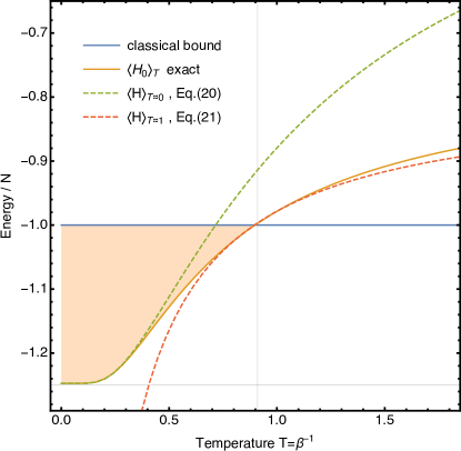
Even if the low temperature approximation Eq. (19) is not suited to describe the regime around the critical temperature, it enables us to study the maximum quantum violation of the inequality we considered. Note that the ground state energy of the system, in the limit , tends to
| (30) |
which coincides with the quantum bound of Ineq. (25), as proven in Ref. [39].
6 Conclusions
We have introduced a framework for the study of Bell correlations in a wide class of spin models at finite temperature. This allowed us to show that nonlocal correlations appear naturally in many-body spin systems, when the temperature is below a critical threshold .
Our results show a clear connection between two-body permutationally invariant Bell inequalities and bosonic systems, via the Holstein-Primakoff approximation and the Bogouliubov transformation. In particular, the low-end part of the spectrum of the Bell operator corresponding to the measurements leading to the maximal quantum violation of the Bell inequality, can be well approximated by a quantum harmonic oscillator, thus extremely simplifying the analysis.
Our work also proves that spin-squeezed states are asymptotically the optimal ones for the class of Bell inequalities (25). Therefore, the quantum states that were prepared in previous experiments detecting Bell correlations in many-body systems belonged to that optimal class (spin-squeezed BEC [49] or thermal ensemble of atoms [50]).
Although, for simplicity, we introduced here our framework with a specific Bell inequality (cf. Ineq (25)), it can easily be generalized. Of special interest would be to find other inequalities that allow to detect Bell correlations within a larger range of temperatures, and generalizations to inequalities with more measurement settings [41] would constitute a good candidate for this task.
We leave as an open problem also the generalization to systems of larger spin. To the best of our knowledge, currently there is no many-body Bell inequality suited to e.g. spin-1 systems, and one would need to resort to methods based on SDP hierarchies to plausibly obtain them [40].
7 Acknowledgments
We are grateful to Roman Schmied for the useful discussions and for the help with the numerical code. M. F. was supported by the Swiss National Science Foundation through Grant No 200020_169591. This project has received funding from the European Union’s Horizon 2020 research and innovation programme under the Marie-Skłodowska-Curie grant agreement No 748549.
References
- Bell [1964] J. S. Bell, Physics 1, 195 (1964).
- Fine [1982] A. Fine, Phys. Rev. Lett. 48, 291 (1982).
- Brunner et al. [2014] N. Brunner, D. Cavalcanti, S. Pironio, V. Scarani, and S. Wehner, Rev. Mod. Phys. 86, 419 (2014).
- Acín et al. [2007] A. Acín, N. Brunner, N. Gisin, S. Massar, S. Pironio, and V. Scarani, Phys. Rev. Lett. 98, 230501 (2007).
- Pironio et al. [2009] S. Pironio, A. Acín, N. Brunner, N. Gisin, S. Massar, and V. Scarani, New Journal of Physics 11, 045021 (2009).
- Colbeck and Renner [2012] R. Colbeck and R. Renner, Nature Physics 8, 450 (2012).
- Pironio et al. [2010] S. Pironio, A. Acín, S. Massar, A. B. de la Giroday, D. N. Matsukevich, P. Maunz, S. Olmschenk, D. Hayes, L. Luo, T. A. Manning, and C. Monroe, Nature 464, 1021 (2010).
- Mayers and Yao [2004] D. Mayers and A. Yao, Quantum Information & Computation 4, 273 (2004).
- Coladangelo et al. [2017] A. Coladangelo, K. T. Goh, and V. Scarani, Nature Communications 8, 15485 (2017), article.
- Salavrakos et al. [2017] A. Salavrakos, R. Augusiak, J. Tura, P. Wittek, A. Acín, and S. Pironio, Phys. Rev. Lett. 119, 040402 (2017).
- Horodecki et al. [2009] R. Horodecki, P. Horodecki, M. Horodecki, and K. Horodecki, Rev. Mod. Phys. 81, 865 (2009).
- Werner [1989] R. F. Werner, Phys. Rev. A 40, 4277 (1989).
- Augusiak et al. [2015] R. Augusiak, M. Demianowicz, J. Tura, and A. Acín, Phys. Rev. Lett. 115, 030404 (2015).
- Bowles et al. [2016] J. Bowles, J. Francfort, M. Fillettaz, F. Hirsch, and N. Brunner, Phys. Rev. Lett. 116, 130401 (2016).
- Augusiak et al. [2018] R. Augusiak, M. Demianowicz, and J. Tura, Phys. Rev. A 98, 012321 (2018).
- Augusiak et al. [2014] R. Augusiak, M. Demianowicz, and A. Acín, Journal of Physics A: Mathematical and Theoretical 47, 424002 (2014).
- Amico et al. [2008] L. Amico, R. Fazio, A. Osterloh, and V. Vedral, Rev. Mod. Phys. 80, 517 (2008).
- Vojta [2003] M. Vojta, Reports on Progress in Physics 66, 2069 (2003).
- Nelson [1988] D. R. Nelson, Phys. Rev. Lett. 60, 1973 (1988).
- Ryu and Takayanagi [2006] S. Ryu and T. Takayanagi, Phys. Rev. Lett. 96, 181602 (2006).
- Lanyon et al. [2010] B. P. Lanyon, J. D. Whitfield, G. G. Gillett, M. E. Goggin, M. P. Almeida, I. Kassal, J. D. Biamonte, M. Mohseni, B. J. Powell, M. Barbieri, A. Aspuru-Guzik, and A. G. White, Nature Chemistry 2, 106 (2010), article.
- Szalay et al. [2015] S. Szalay, M. Pfeffer, V. Murg, G. Barcza, F. Verstraete, R. Schneider, and Örs Legeza, International Journal of Quantum Chemistry 115, 1342 (2015).
- Verstraete et al. [2008] F. Verstraete, V. Murg, and J. Cirac, Advances in Physics 57, 143 (2008).
- Liu et al. [2017] D. Liu, S.-J. Ran, P. Wittek, C. Peng, R. B. García, G. Su, and M. Lewenstein, “Machine learning by two-dimensional hierarchical tensor networks: A quantum information theoretic perspective on deep architectures,” (2017), arXiv:1710.04833 .
- Pitowsky [1989] I. Pitowsky, Quantum Probability – Quantum Logic, Lecture Notes in Physics (Springer-Verlag Berlin Heidelberg, 1989).
- Babai et al. [1991] L. Babai, L. Fortnow, and C. Lund, computational complexity 1, 3 (1991).
- Mermin [1990] N. D. Mermin, Phys. Rev. Lett. 65, 1838 (1990).
- Werner and Wolf [2001] R. F. Werner and M. M. Wolf, Phys. Rev. A 64, 032112 (2001).
- Żukowski and Brukner [2002] M. Żukowski and i. c. v. Brukner, Phys. Rev. Lett. 88, 210401 (2002).
- Bancal et al. [2011] J.-D. Bancal, N. Brunner, N. Gisin, and Y.-C. Liang, Phys. Rev. Lett. 106, 020405 (2011).
- Chen et al. [2011] J.-L. Chen, D.-L. Deng, H.-Y. Su, C. Wu, and C. H. Oh, Phys. Rev. A 83, 022316 (2011).
- Gühne et al. [2005] O. Gühne, G. Tóth, P. Hyllus, and H. J. Briegel, Phys. Rev. Lett. 95, 120405 (2005).
- Tóth et al. [2006] G. Tóth, O. Gühne, and H. J. Briegel, Phys. Rev. A 73, 022303 (2006).
- Cavalcanti et al. [2007] E. G. Cavalcanti, C. J. Foster, M. D. Reid, and P. D. Drummond, Phys. Rev. Lett. 99, 210405 (2007).
- He et al. [2009] Q. Y. He, E. G. Cavalcanti, M. D. Reid, and P. D. Drummond, Phys. Rev. Lett. 103, 180402 (2009).
- He et al. [2010] Q. Y. He, E. G. Cavalcanti, M. D. Reid, and P. D. Drummond, Phys. Rev. A 81, 062106 (2010).
- Salles et al. [2010] A. Salles, D. Cavalcanti, A. Acin, D. Perez-Garcia, and M. M. Wolf, Quantum Information and Computation 10, 0703 (2010).
- Tura et al. [2014a] J. Tura, R. Augusiak, A. B. Sainz, T. Vértesi, M. Lewenstein, and A. Acín, Science 344, 1256 (2014a).
- Tura et al. [2015] J. Tura, R. Augusiak, A. Sainz, B. Lücke, C. Klempt, M. Lewenstein, and A. Acín, Annals of Physics 362, 370 (2015).
- Fadel and Tura [2017] M. Fadel and J. Tura, Phys. Rev. Lett. 119, 230402 (2017).
- Wagner et al. [2017] S. Wagner, R. Schmied, M. Fadel, P. Treutlein, N. Sangouard, and J.-D. Bancal, Phys. Rev. Lett. 119, 170403 (2017).
- Tura et al. [2017] J. Tura, G. De las Cuevas, R. Augusiak, M. Lewenstein, A. Acín, and J. I. Cirac, Phys. Rev. X 7, 021005 (2017).
- Tura et al. [2014b] J. Tura, A. B. Sainz, T. Vértesi, A. Acín, M. Lewenstein, and R. Augusiak, Journal of Physics A: Mathematical and Theoretical 47, 424024 (2014b).
- Wang et al. [2017] Z. Wang, S. Singh, and M. Navascués, Phys. Rev. Lett. 118, 230401 (2017).
- Wang and Navascués [2018] Z. Wang and M. Navascués, Proceedings of the Royal Society of London A 474 (2018).
- Baccari et al. [2017] F. Baccari, D. Cavalcanti, P. Wittek, and A. Acín, Phys. Rev. X 7, 021042 (2017).
- Sorensen et al. [2001] A. Sorensen, L.-M. Duan, J. I. Cirac, and P. Zoller, Nature 409, 63 (2001).
- Eckert et al. [2008] K. Eckert, O. Romero-Isart, M. Rodriguez, M. Lewenstein, E. S. Polzik, and A. Sanpera, Nat Phys 4, 50 (2008).
- Schmied et al. [2016] R. Schmied, J.-D. Bancal, B. Allard, M. Fadel, V. Scarani, P. Treutlein, and N. Sangouard, Science 352, 441 (2016).
- Engelsen et al. [2017] N. J. Engelsen, R. Krishnakumar, O. Hosten, and M. A. Kasevich, Phys. Rev. Lett. 118, 140401 (2017).
- Estève et al. [2008] J. Estève, C. Gross, A. Weller, S. Giovanazzi, and M. K. Oberthaler, Nature 455, 1216 (2008).
- Gross et al. [2010] C. Gross, T. Zibold, E. Nicklas, J. Estève, and M. K. Oberthaler, Nature 464, 1165 (2010).
- Riedel et al. [2010] M. F. Riedel, P. Böhi, Y. Li, T. W. Hänsch, A. Sinatra, and P. Treutlein, Nature 464, 1170 (2010).
- Leroux et al. [2010] I. D. Leroux, M. H. Schleier-Smith, and V. Vuletić, Phys. Rev. Lett. 104, 073602 (2010).
- Britton et al. [2012] J. W. Britton, B. C. Sawyer, A. C. Keith, C. C. J. Wang, J. K. Freericks, H. Uys, M. J. Biercuk, and J. J. Bollinger, Nature 484, 489 (2012).
- Bohnet et al. [2016] J. G. Bohnet, B. C. Sawyer, J. W. Britton, M. L. Wall, A. M. Rey, M. Foss-Feig, and J. J. Bollinger, Science 352, 1297 (2016).
- Holstein and Primakoff [1940] T. Holstein and H. Primakoff, Phys. Rev. 58, 1098 (1940).
- Bogoljubov [1958] N. N. Bogoljubov, Il Nuovo Cimento (1955-1965) 7, 794 (1958).
- Valatin [1958] J. G. Valatin, Il Nuovo Cimento (1955-1965) 7, 843 (1958).
- Moroder et al. [2012] T. Moroder, P. Hyllus, G. Tóth, C. Schwemmer, A. Niggebaum, S. Gaile, O. Gühne, and H. Weinfurter, New Journal of Physics 14, 105001 (2012).
- i Brugués [2017] J. T. i Brugués, Characterizing Entanglement and Quantum Correlations Constrained by Symmetry (Springer International Publishing, 2017).
- Christandl [2006] M. Christandl, The Structure of Bipartite Quantum States - Insights from Group Theory and Cryptography, Ph.D. thesis, University of Cambridge (2006).
- Harrow [2005] A. Harrow, Applications of coherent classical communication and the Schur transform to quantum information theory, Ph.D. thesis, Massachusetts Institute of Technology, Cambridge, MA (2005).
- Audenaert [2006] K. Audenaert, “A digest on representation theory of the symmetric group,” (2006).
- Toner and Verstraete [2006] B. Toner and F. Verstraete, “Monogamy of bell correlations and tsirelson’s bound,” (2006), arXiv:quant-ph/0611001 .
8 Appendix
We give here the expression for the approximated partition function, valid around for . For and we find
| (31) |
