iSTRICT: An Interdependent Strategic Trust Mechanism for the Cloud-Enabled Internet of Controlled Things

Abstract

The cloud-enabled Internet of controlled things (IoCT) envisions a network of sensors, controllers, and actuators connected through a local cloud in order to intelligently control physical devices. Because cloud services are vulnerable to advanced persistent threats (APTs), each device in the IoCT must strategically decide whether to trust cloud services that may be compromised. In this paper, we present iSTRICT, an interdependent strategic trust mechanism for the cloud-enabled IoCT. iSTRICT is composed of three interdependent layers. In the cloud layer, iSTRICT uses FlipIt games to conceptualize APTs. In the communication layer, it captures the interaction between devices and the cloud using signaling games. In the physical layer, iSTRICT uses optimal control to quantify the utilities in the higher level games. Best response dynamics link the three layers in an overall “game-of-games,” for which the outcome is captured by a concept called Gestalt Nash equilibrium (GNE). We prove the existence of a GNE under a set of natural assumptions and develop an adaptive algorithm to iteratively compute the equilibrium. Finally, we apply iSTRICT to trust management for autonomous vehicles that rely on measurements from remote sources. We show that strategic trust in the communication layer achieves a worst-case probability of compromise for any attack and defense costs in the cyber layer.

I Introduction

The Internet of Things (IoT) will impact a diverse set of consumer, public sector, and industrial systems. Smart homes and buildings, autonomous vehicles and transportation [1], and the interaction between wearable fitness devices and social networks [2] provide a few examples of application areas which will be particularly impacted by the IoT. One definition of the IoT is a “dynamic global network infrastructure with self-configuring capabilities based on standard and interoperable communication protocols where physical and virtual ‘things’ have identities, physical attributes, and virtual personalities” [3]. This definition envisions a decentralized, heterogeneous network with plug-and-play capabilities. The related concept of cyber-physical systems (CPS) refers to “smart networked systems with embedded sensors, processors, and actuators” [4]. [5] provides a detailed introduction to CPS and reports on its development status. The term CPS emphasizes the “systems” nature of these networks. In both IoT and CPS, “the joint behavior of the ‘cyber’ and physical elements of the system is critical—computing, control, sensing, and networking can be integrated into every component” [4]. The importance of sensing, actuation, and control to devices in the IoT has given rise to the term “Internet of controlled things,” or IoCT. Hereafter, we refer to the IoCT as a way to address challenges of both CPS and IoT.

The IoCT requires an interface between heterogeneous components. Local clouds (or fogs or cloudlets) offer promising solutions. In these networks, a cloud provides services for data aggregation, data storage, and computation. In addition, the cloud provides a market for the services of software developers and computational intelligence experts [6]. Figure 1 depicts a cloud-enabled IoCT. In this network, sensors push environment data to the cloud, where it is aggregated and sent to devices (or “things”), which use the data for feedback control. These devices modify the environment, and the cycle continues. Note that the control design of the IoCT is distributed, since each device can determine which cloud services to use for feedback control.

Figure 1: iSTRICT addresses security and trust issues for a cloud-enabled IoCT. The cloud-enabled IoCT consists of connected sensors and devices, with a cloud as the interface. Adversaries are capable of compromising cloud services and modifying the control signals that they transmit to the devices. The trust issue lies between the cloud (sender) and IoCT (receiver). Each IoCT device should determine which signals to trust from cloud services strategically.

I-A Advanced Persistent Threats in the Cloud-Enabled IoCT

Unfortunately, cyberattacks on the cloud are increasing as more businesses utilize cloud services [7]. To provide reliable support for IoCT applications, sensitive data provided by the cloud services needs to be well protected [8]. In this paper we focus on the attack model of advanced persistent threats (APTs): “cyber attacks executed by sophisticated and well-resourced adversaries targeting specific information in high-profile companies and governments, usually in a long term campaign involving different steps” [9]. In the initial stage of an APT, an attacker penetrates the network through techniques such as social engineering, malicious hardware injection, theft of cryptographic keys, or zero-day exploits [10]. For example, the Naikon APT, which targeted governments around the South China Sea in 2010-2015, used a bait document that appeared to be a Microsoft Word file but which was actually a malicious executable that installed spware [11]. The cloud is particularly vulnerable to initial penetration through application-layer attacks, because many applications are required for developers and clients to interface with the cloud. Our iSTRICT can be applied to many cyberattack scenarios. For example, cross-site scripting (XSS) and SQL injection are two types of application-layer attacks. In SQL injection, attackers insert malicious SQL code into fields which do not properly process string literal escape characters. The malicious code targets the server, where it could be used to modify data or bypass authentication systems. By contrast, XSS targets the execution of code in the browser on the client side. All of these attacks give attackers an initial entry point into a system, from which they can begin to gain more complete, insider control. This control of the cloud can be used to transmit malicious signals to CPS and cause physical damage.

I-B Strategic Trust

Given the threat of insider attacks on the cloud, each IoCT device must decide which signals to trust from cloud services. Trust refers to positive beliefs about the perceived reliability of, dependability of, and confidence in another entity [12]. These entities may be agents in an IoCT with misaligned incentives. Many specific processes in the IoCT require trust, such as data collection, aggregation and processing, privacy protection, and user-device trust in human-in-the-loop interactions [13]. While many factors influence trust, including subjective beliefs, we focus on objective properties of trust. These include 1) reputation, 2) promises, and 3) interaction context. Many trust management systems are based on tracking reputation over multiple interactions. Unfortunately, agents in the IoCT may interact only once, making reputation difficult to accrue [14]. This property of IoCT also limits the effectiveness of promises such as contracts or policies. Promises may not be enforceable for entities that interact only once. Therefore we focus on strategic trust that is predictive rather than reactive. We use game-theoretic utility functions to capture the motivations for entities to be trustworthy. These utility functions change based on the particular context of the interaction. In this sense, our model of strategic trust is incentive-compatible, i.e., consistent with each agent acting in its own self-interest.

I-C Game-Theoretic iSTRICT Model

We propose a framework called iSTRICT, which is composed of three interacting layers: a cloud layer, a communication layer, and a physical layer. In the first layer, the cloud-services are threatened by attackers capable of APTs and defended by network administrators (or “defenders”). The interaction at each cloud-service is modeled using the FlipIt game recently proposed by Bowers et al. [10] and van Dijk et al. [15]. iSTRICT uses one FlipIt game per cloud-service. In the communication layer, the cloud-services—which may be controlled by the attacker or defender according to the outcome of the FlipIt game—transmit information to a device which decides whether to trust the cloud-services. This interaction is captured using a signaling game. At the physical layer, the utility parameters for the signaling game are determined using optimal control. The cloud, communication, and physical layers are interdependent. This motivates an overall equilibrium concept called Gestalt Nash equilibrium (GNE). GNE requires each game to be solved optimally given the results of the other games. Because this is a similar idea to best-response in Nash equilibrium, we call the multi-game framework a game-of-games.

I-D Contributions

In summary, we present the following contributions:

1. Trust Model: We develop a multi-layer framework (iSTRICT) and associated equilibrium concept (GNE) to capture interdependent strategic trust in the cloud-enabled IoCT. iSTRICT combines analysis at the cloud, communication, and physical layers.

2. GNE Analysis: We prove the existence of GNE, and we show that strategic trust in the communication layer guarantees a worst-case probability of compromise regardless of attack costs in the cyber layer.

3. Adaptive Algorithm: We present an adaptive algorithm using best-response dynamics to compute a GNE.

4. Autonomous Vehicle Application: We simulate the control of a pair of autonomous vehicles using iSTRICT, and show improvement over the performance under naive policies.

The rest of the paper proceeds as follows. In Section II, we give a broad outline of the iSTRICT model. Section III presents the details of the FlipIt game, signaling game, physical layer control system, and equilibrium concept. Then, in Section IV, we study the equilibrium analytically using an adaptive algorithm. Finally, we apply the framework to the control of autonomous vehicles in Section V.

I-E Related Work

Designing trustworthy cloud service systems has been investigated extensively in the literature. Various methods, including a feedback evaluation component, Bayesian game, and domain partition have been proposed [16, 17, 18]. Trust models to predict the cloud trust values (or reputation) can be mainly divided into objective and subjective classes. The first are based on the quality of service parameters, and the second are based on feedback from cloud service users [16, 19].

In the IoCT, however, agents may not have sufficient number of interactions, which makes reputation challenging to obtain [14]. In addition, trust value-based cloud trust management systems can be compromised by reputation attacks through fake feedback which can severely degrade the system performance [16, 20]. Therefore, in this work, we aim to design a strategic trust mechanism which is predictive rather than reactive through an integrative game-theoretic framework. Rather than using trust value [21, 20], IoCT devices in our iSTRICT model make decisions based on the strategies of players at the cloud layer as well as based on the physical system performance. This multi-layer design provides resilience to reputation attacks.

Cyber-physical systems security becomes a critical concern due to the prevailing threats from both cyber and physical components in the system [22, 23, 24]. To facilitate a secure system design, game theory has been widely adopted to model and capture the strategic interactions between the attackers and defenders [25, 26, 27]. Our iSTRICT framework builds on two existing game models. One is the signaling game which has been used in intrusion detection systems [28] and network defense [29]. The other one is the FlipIt game [10, 15] which has been applied to security of a single cloud service [25, 30] as well as AND/OR combinations of cloud services [31]. In contrast to previous works, in this paper we propose a three-layer interdependent model to enable devices to decide whether to trust cloud services that may be compromised. Specifically, trust management decisions are coupled by the dynamics of cloud-enabled devices, because data provided by the cloud services is used for feedback control. Devices must balance the need for as many data sources as possible (in order to increase the quality of the feedback control) with the imperative to reject data sources that are compromised by attackers.

In terms of the technical framework, iSTRICT builds on existing achievements in IoCT architecture design [6, 32, 33, 34], which describe the roles of different layers of the IoCT at which data is collected, processed, and accessed by devices [33]. Each layer of the IoCT consists of different enabling technologies such as wireless sensor networks and data management systems [34]. Our perspective, however, is distinct from this literature because we emphasize an integrated mathematical framework. iSTRICT leverages game theory to obtain optimal defense strategies for IoCT components, and it uses control theory to quantify the performance of devices.

II iSTRICT Overview

We consider a cyber-physical attack in which an adversary penetrates a cloud service in order to transmit malicious signals to a physical device and cause improper operation. This type of cross-layer attack is increasingly relevant in IoCT settings. Perhaps the most famous cross-layer attack is the Stuxnet attack that damaged Iran’s nuclear program. But even more recently, an attacker allegedly penetrated the supervisory control and data acquisition (SCADA) system that controls the Bowman Dam, located less than $20$ miles north of Manhattan. The attacker gained control of a sluice gate which manages water level [35]. Cyber-physical systems ranging from the smart grid to public transportation need to be protected from similar attacks.

The iSTRICT framework offers a defense-in-depth approach to IoCT security. In this section, we introduce each of the three layers of iSTRICT very briefly, in order to focus on the interaction between the layers. We describe an equilibrium concept for the simultaneous steady-state of all three layers. Later, Section III describes each layer in detail. Table I lists the notation for the paper.

TABLE I: Nomenclature

Notation	Meaning
$\mathbb{S}=\{1,2,\ldots,N\}$	Cloud services (CSs)
$\mathcal{A}^{i},$ $\mathcal{D}^{i},$ $i\in\mathbb{S},$ $\mathcal{R}$	Attackers, defenders, device
$v_{\mathcal{A}}=[v_{\mathcal{A}}^{i}]_{i\in\mathbb{S}}$	Values of CSs for $\mathcal{A}$
$v_{\mathcal{D}}=[v_{\mathcal{D}}^{i}]_{i\in\mathbb{S}}$	Values of CSs for $\mathcal{D}$
$p_{\mathcal{A}}=[p_{\mathcal{A}}^{i}]_{i\in\mathbb{S}}$	Probabilities that $\mathcal{A}$ controls CSs
$p_{\mathcal{D}}=[p_{\mathcal{D}}^{i}]_{i\in\mathbb{S}}$	Probabilities that $\mathcal{D}$ controls CSs
$p_{\mathcal{A}}^{i*}=T^{F_{i}}(v_{\mathcal{A}}^{i},v_{\mathcal{D}}^{i})$	FlipIt mapping for CS $i$
$(v_{\mathcal{A}}^{*},v_{\mathcal{D}}^{*})\in T^{S}(p_{\mathcal{A}})$	Signaling game mapping
$f_{\mathcal{A}}^{i},$ $f_{\mathcal{D}}^{i}$	Frequencies $\mathcal{A}^{i}$ and $\mathcal{D}^{i}$
$u_{\mathcal{A}}^{F_{i}}(f_{\mathcal{A}}^{i},f_{\mathcal{D}}^{i})$	$\mathcal{A}^{i}$’s utility in FlipIt game $i$
$u_{\mathcal{D}}^{F_{i}}(f_{\mathcal{A}}^{i},f_{\mathcal{D}}^{i})$	$\mathcal{D}^{i}$’s utility in FlipIt game $i$
$\theta=[\theta^{i}]_{i\in\mathbb{S}}$	Types of CSs
$\theta^{i}\in\Theta=\{\theta_{\mathcal{A}},\theta_{\mathcal{D}}\}$	Type spaces of CSs
$m=[m^{i}]_{i\in\mathbb{S}}$	Messages from CSs
$m^{i}\in M=\{m_{L},m_{H}\}$	Low or high risk message
$a=[a^{i}]_{i\in\mathbb{S}}$	Actions for CSs
$a^{i}\in A=\{a_{T},a_{N}\}$	Trust or not trust action
$u_{\mathcal{A}}^{S_{i}}(m,a),$ $u_{\mathcal{D}}^{S_{i}}(m,a)$	Signaling game utility of $\mathcal{A}^{i}$ and $\mathcal{D}^{i}$
$u_{\mathcal{R}}^{S}(\theta,m,a)$	Signaling game utility for $\mathcal{R}$
$\sigma_{\mathcal{A}}^{i}(m)\in\Sigma_{\mathcal{A}}$	Signaling game mixed strategies of $\mathcal{A}^{i}$
$\sigma_{\mathcal{D}}^{i}(m)\in\Sigma_{\mathcal{D}}$	Signaling game mixed strategies of $\mathcal{D}^{i}$
$\sigma_{\mathcal{R}}(a\,|\,m)\in\Sigma_{\mathcal{R}}^{N}$	Signaling game mixed strategy for $\mathcal{R}$
$\mu(\theta\,|\,m)=[\mu^{i}(\theta\,|\,m)]_{i\in\mathbb{S}}$	Beliefs of $\mathcal{R}$ about CSs
$\bar{u}_{\mathcal{A}}^{S_{i}}(\sigma_{\mathcal{R}};\sigma_{\mathcal{A}}^{i},\sigma_{\mathcal{A}}^{-i};\sigma_{\mathcal{D}}^{-i})$	Signaling game utility for $\mathcal{A}^{i}$
$\bar{u}_{\mathcal{D}}^{S_{i}}(\sigma_{\mathcal{R}};\sigma_{\mathcal{A}}^{-i};\sigma_{\mathcal{D}}^{i},\sigma_{\mathcal{D}}^{-i})$	Signaling game utility for $\mathcal{D}^{i}$
$x[k],$ $\hat{x}[k],$ $u[k],$	State, estimated state, control
$\Delta_{\mathcal{A}}^{i}[k],$ $\Delta_{\mathcal{D}}^{i}[k],$	bias terms of $\mathcal{A}^{i}$ and $\mathcal{D}^{i}$
$\Xi_{\theta}[k]$	cloud type matrix
$y[k],$ $\tilde{y}[k],$	Measurements without and with biases
$\xi,$ $\zeta$	Covariance matrices of noises
$\nu[k],$ $\epsilon$	Innovation, innovation thresholds
$D_{\sigma_{\mathcal{R}}}(\nu[k])$	Innovation gate
$v_{\mathcal{A}\mathcal{D}}^{i}=v_{\mathcal{A}}^{i}/v_{\mathcal{D}}^{i},$ $i\in\mathbb{S}$	Ratios of CSs’ value for $\mathcal{A}^{i}$ and $\mathcal{D}^{i}$
$\mathbb{V}^{i},$ $\mathbb{PR}^{i}$	Spaces of $v_{\mathcal{A}\mathcal{D}}^{i}$ and $p_{\mathcal{A}}^{i}$ in a GNE
$p_{\mathcal{A}}^{i*}=\tilde{T}^{F_{i}}(v_{\mathcal{A}\mathcal{D}}^{i})$	Redefined FlipIt mapping for CS $i$
$v_{\mathcal{A}\mathcal{D}}^{*}\in\tilde{T}^{S}(p_{\mathcal{A}})$	Redefined signaling game mapping
$v_{\mathcal{A}\mathcal{D}}^{*}\in\tilde{T}^{S\circ F}(v_{\mathcal{A}\mathcal{D}})$	Composition of $\tilde{T}^{F_{i}},$ $i\in\mathbb{S}$ and $\tilde{T}^{S}$
$v_{\mathcal{A}\mathcal{D}}^{\dagger}\in\tilde{T}^{S\circ F}(v_{\mathcal{A}\mathcal{D}}^{\dagger})$	Fixed-point requirement for a GNE

II-A Cloud Layer

Consider a cloud-enabled IoCT composed of sensors that push data to a cloud, which aggregates the data and sends it to devices. For example, in a cloud-enabled smart home, sensors could include lighting sensors, temperature sensors, and blood pressure or heart rate sensors that may be placed on the skin or embedded within the body. Data from these sensors is processed by a set of cloud services $\mathbb{S}=\left\{1,\ldots,N\right\},$ which make data available for control.

For each cloud service $i\in\mathbb{S},$ let $\mathcal{A}^{i}$ denote an attacker who attempts to penetrate the service using zero-day exploits, social engineering, or other techniques described in Section I. Similarly, let $\mathcal{D}^{i}$ denote a defender or network administrator attempting to maintain the security of the cloud service. $\mathcal{A}^{i}$ and $\mathcal{D}^{i}$ attempt to claim or reclaim control of the each cloud service at periodic intervals. We model the interactions at all of the services using FlipIt games, one for each of the $N$ services.

In the FlipIt game [10, 15], an attacker and a defender gain utility proportional to the amount of time that they control a resource (here a cloud service), and pay attack costs proportional to the number of times that they attempt to claim or reclaim the resource. We consider a version of the game in which the attacker and defender are restricted to attacking at fixed frequencies. The equilibrium of the game is a Nash equilibrium.

Let $v_{\mathcal{A}}^{i}\in\mathbb{R}$ and $v_{\mathcal{D}}^{i}\in\mathbb{R}$ denote the values of each cloud service $i\in\mathbb{S}$ to $\mathcal{A}^{i}$ and $\mathcal{D}^{i},$ respectively. These quantities represent the inputs of the FlipIt game. The outputs of the FlipIt game are the proportions of time for which $\mathcal{A}^{i}$ and $\mathcal{D}^{i}$ control the cloud service. Denote these proportions by $p_{\mathcal{A}}^{i}\in\left[0,1\right]$ and $p_{\mathcal{D}}^{i}=1-p_{\mathcal{A}}^{i},$ respectively. To summarize each of the FlipIt games, define a set of mappings $T^{F_{i}}:\,\mathbb{R}\times\mathbb{R}\to\left[0,1\right],$ $i\in\mathbb{S},$ such that

$$p_{\mathcal{A}}^{i*}=T^{F_{i}}\left(v_{\mathcal{A}}^{i},v_{\mathcal{D}}^{i}\right)$$ (1)

maps the values of cloud service $i$ for $\mathcal{A}^{i}$ and $\mathcal{D}^{i}$ to the proportion of time $p_{\mathcal{A}}^{i*}$ for which the service will be compromised in equilibrium. We will study this mapping further in Section III-A.

II-B Communication Layer

In the communication layer, the cloud services $i\in\mathbb{S},$ which each may be controlled by $\mathcal{A}^{i}$ or $\mathcal{D}^{i},$ send data to a device $\mathcal{R},$ which decides whether to trust the signals. This interaction is modeled by a signaling game. The signaling game sender is the cloud service. The two types of the sender are attacker or defender. The signaling game receiver is the device $\mathcal{R}.$ While we used $N$ FlipIt games to describe the cloud layer, we use only one signaling game to describe the communication layer, because $\mathcal{R}$ must decide which services to trust all at once.

The prior probabilities in the communication layer are the equilibrium proportions $p_{\mathcal{A}}^{i}$ and $p_{\mathcal{D}}^{i}=1-p_{\mathcal{A}}^{i},$ $i\in\mathbb{S}$ from the equilibrium of the cloud layer. Denote the vectors of the prior probabilities for each sensor by $p_{\mathcal{A}}=\left[p_{\mathcal{A}}^{i}\right]_{i\in\mathbb{S}},$ $p_{\mathcal{D}}=\left[p_{\mathcal{D}}^{i}\right]_{i\in\mathbb{S}}.$ These prior probabilities are the inputs of the signaling game.

The outputs of the signaling game are the equilibrium utilities received by the senders. Denote these utilities by $v_{\mathcal{A}}^{i}$ and $v_{\mathcal{D}}^{i},$ $i\in\mathbb{S}.$ Importantly, these are the same quantities that describe the incentives of $\mathcal{A}$ and $\mathcal{D}$ to control each cloud service in the FlipIt game, because the party which controls each service is awarded the opportunity to be the sender in the signaling game. Define vectors to represent each of these utilities by $v_{\mathcal{A}}=\left[v_{\mathcal{A}}^{i}\right]_{i\in\mathbb{S}},$ $v_{\mathcal{D}}=\left[v_{\mathcal{D}}^{i}\right]_{i\in\mathbb{S}}.$

Finally, let $T^{S}:\,\left[0,1\right]^{N}\to\mathcal{P}(\mathbb{R}^{2N})$ be a mapping that summarizes the signaling game, where $\mathcal{P}(\mathbb{X})$ is the power set of $\mathbb{X}.$ According to this mapping, the set of vectors of signaling game equilibrium utility ratios $v_{\mathcal{A}}^{*}$ and $v_{\mathcal{D}}^{*}$ that result from the vector of prior probabilities $p_{\mathcal{A}}$ is given by

$$\left(v_{\mathcal{A}}^{*},v_{\mathcal{D}}^{*}\right)=T^{S}\left(p_{\mathcal{A}}\right).$$ (2)

This mapping summarizes the signaling game. We study the mapping in detail in Section III-B.

II-C Physical Layer

Many IoCT devices such as pacemakers, cleaning robots, appliances, and electric vehicles are dynamic systems that operate using feedback mechanisms. The physical-layer control of these devices requires remote sensing of the environment and the data stored or processed in the cloud. The security at the cloud and the communication layers of the system are intertwined with the performance of the controlled devices at the physical layer. Therefore the trustworthiness of the data has a direct impact on the control performance of the devices. This control performance determines the utility of the device $\mathcal{R}$ as well as the utility of each of the attackers $\mathcal{A}^{i}$ and defenders $\mathcal{D}^{i}.$ The control performance is quantified using a cost criterion for observer-based optimal feedback control. The observer uses data from the cloud services that $\mathcal{R}$ elects to trust, and ignores the cloud services that $\mathcal{R}$ decides not to trust. We study the physical layer control in Section III-C.

II-D Coupling of the Cloud and Communication Layers

Figure 2: In iSTRICT, FlipIt games model attacks on the set of cloud services. $T^{F_{i}},$ $i\in\mathbb{S},$ map the value of each service to the proportion of time that it will be compromised in equilibrium. The communication layer is modeled by a signaling game. $T^{S}$ maps probabilities of compromise to the value of each cloud service. The cloud layer and communication layer are interdependent. The physical layer performance quantifies the utilities for the signaling game.

Clearly, the cloud and communication layers are coupled through Eq. (1) and Eq. (2). The cloud layer security serves as an input to the communication layer. The resulting utilities of the signaling game at the communication layer further becomes an input to the FlipIt game at the cloud layer. In addition, the physical layer performance quantifies the utilities for the signaling games. Fig. 2 depicts this concept. In order to predict the behavior of the whole cloud-enabled IoCT, iSTRICT considers an equilibrium concept which we call Gestalt Nash equilibrium (GNE). Informally, a triple $\left(p_{\mathcal{A}}^{\dagger},v_{\mathcal{A}}^{\dagger},v_{\mathcal{D}}^{\dagger}\right)$ is a GNE if it simultaneously satisfies Eq. (1) and Eq. (2).

GNE is useful for three reasons. First, cloud-enabled IoCT networks are dynamic. The modular structure of GNE requires the FlipIt games and the signaling game to be at equilibrium given the parameters that they receive from the other type of game. This imposes the requirement of perfection, in the sense that each game must be optimal given the other game. In GNE, perfection applies in both directions, because there is no clear chronological order or directional flow of information between the two games. Actions in each sub-game must be chosen by prior-commitment relative to the results of the other sub-game.

Second, GNE draws upon established results from FlipIt games and signaling games instead of attempting to analyze one large game. IoCT networks promise plug-and-play capabilities, in which devices and users are easily able to enter and leave the network. This also motivates plug-and-play availability of solution concepts. The solution to one sub-game should not need to be totally recomputed if an actor enters or leaves another subgame. GNE follows this approach.

Finally, GNE serves as an example of a solution approach which could be called game-of-games. The equilibrium solutions to the FlipIt games and signaling game must be rational “best responses” to the solution of the other type of game.

III Detailed iSTRICT Model

In this section, we define more precisely the three layers of the iSTRICT framework.

III-A Cloud Layer: FlipIt Game

We use a FlipIt game to model the interactions between the attacker and the defender over each cloud service.

III-A1 FlipIt Actions

For each service, $\mathcal{A}^{i}$ and $\mathcal{D}^{i}$ choose $f_{\mathcal{A}}^{i}$ and $f_{\mathcal{D}}^{i},$ the frequencies with which they claim or reclaim control of the service. These frequencies are chosen by prior commitment. Neither player knows the other player’s action when she makes her choice. Figure 3 depicts the FlipIt game. The green boxes above the horizontal axis represent control of the service by $\mathcal{D}^{i}$ and the red boxes below the axis represent control of the service by $\mathcal{A}^{i}.$

From $f_{\mathcal{A}}^{i}$ and $f_{\mathcal{D}}^{i},$ it is easy to compute the expected proportions of the time that $\mathcal{A}$ and $\mathcal{D}$ control service $i$ [10, 15]. Let $\mathbb{R}_{+}$ denote the set of non-negative real numbers. Define the function $\rho:\,\mathbb{R}_{+}\times\mathbb{R}_{+}\to\left[0,1\right],$ such that $p_{\mathcal{A}}^{i}=\rho\left(f_{\mathcal{A}}^{i},f_{\mathcal{D}}^{i}\right)$ gives the proportion of the time that $\mathcal{A}^{i}$ will control the cloud service if he attacks with frequency $f_{\mathcal{A}}^{i}$ and $\mathcal{D}^{i}$ renews control of the service (through changing cryptographic keys or passwords, or through installing new hardware) with frequency $f_{\mathcal{D}}^{i}.$ We have

$$\rho\left(f_{\mathcal{A}}^{i},f_{\mathcal{D}}^{i}\right)=\begin{cases}0,&\text{ if }f_{\mathcal{A}}^{i}=0,\\ \frac{f_{\mathcal{A}}^{i}}{2f_{\mathcal{D}}^{i}},&\text{ if }f_{\mathcal{D}}^{i}\geq f_{\mathcal{A}}^{i}>0,\\ 1-\frac{f_{\mathcal{D}}^{i}}{2f_{\mathcal{A}}^{i}},&\text{ if }f_{\mathcal{A}}^{i}>f_{\mathcal{D}}^{i}\geq 0.\end{cases}$$ (3)

Notice that when $f_{\mathcal{A}}^{i}>f_{\mathcal{D}}^{i}\geq 0$, i.e., the attacking frequency of $\mathcal{A}^{i}$ is greater than the renewal frequency of $\mathcal{D}^{i}$, the proportion of time that service $i$ is insecure is $\rho\left(f_{\mathcal{A}}^{i},f_{\mathcal{D}}^{i}\right)>\frac{1}{2}$, and when $f_{\mathcal{D}}^{i}\geq f_{\mathcal{A}}^{i}>0$, we obtain $\rho\left(f_{\mathcal{A}}^{i},f_{\mathcal{D}}^{i}\right)\leq\frac{1}{2}$.

III-A2 FlipIt Utility Functions

Recall that $v_{\mathcal{A}}^{i}$ and $v_{\mathcal{D}}^{i}$ denote the value of controlling service $i\in\mathbb{S}$ for $\mathcal{A}^{i}$ and $\mathcal{D}^{i},$ respectively. These quantities define the heights of the red and green boxes in Fig. 3. Denote the costs of renewing control of the cloud service for the two players by $\alpha_{\mathcal{A}}^{i}$ and $\alpha_{\mathcal{D}}^{i}.$ Finally, let $\bar{u}_{\mathcal{A}}^{F_{i}}:\,\mathbb{R}_{+}\times\mathbb{R}_{+}\to\mathbb{R}$ and $\bar{u}_{\mathcal{D}}^{F_{i}}:\,\mathbb{R}_{+}\times\mathbb{R}_{+}\to\mathbb{R}$ be expected utility functions for each FlipIt game. The utilities of each player are given in Eq. (4) and Eq. (5) by the values $v_{\mathcal{D}}^{i}$ and $v_{\mathcal{A}}^{i}$ of controlling the service multiplied by the proportions $p_{\mathcal{D}}^{i}$ and $p_{\mathcal{A}}^{i}$ with which the service is controlled, minus the costs $\alpha_{\mathcal{D}}^{i}$ and $\alpha_{\mathcal{A}}^{i}$ of attempting to renew control of the service.

$$\bar{u}_{\mathcal{D}}^{F_{i}}\left(f_{\mathcal{A}}^{i},f_{\mathcal{D}}^{i}\right)=v_{\mathcal{D}}^{i}\left(1-\rho\left(f_{\mathcal{A}}^{i},f_{\mathcal{D}}^{i}\right)\right)-\alpha_{\mathcal{D}}^{i}f_{\mathcal{D}}^{i}.$$ (4)

$$\bar{u}_{\mathcal{A}}^{F_{i}}\left(f_{\mathcal{A}}^{i},f_{\mathcal{D}}^{i}\right)=v_{\mathcal{A}}^{i}\rho\left(f_{\mathcal{A}}^{i},f_{\mathcal{D}}^{i}\right)-\alpha_{\mathcal{A}}^{i}f_{\mathcal{A}}^{i}.$$ (5)

Therefore, based on the attacker’s action $f_{\mathcal{A}}^{i}$, the defender determines $f_{\mathcal{D}}^{i}$ strategically to maximize the proportional time of controlling the cloud service $i$, $1-\rho(f_{\mathcal{A}}^{i},f_{\mathcal{D}}^{i})$, and minimize the cost of choosing $f_{\mathcal{D}}^{i}$.

Note that in the game, the attacker knows $v_{\mathcal{A}}^{i}$ and $\alpha_{\mathcal{A}}^{i}$, and the defender knows $v_{\mathcal{D}}^{i}$ and $\alpha_{\mathcal{D}}^{i}$. Furthermore, $\rho(f_{\mathcal{A}}^{i},f_{\mathcal{D}}^{i})$ is public information, and hence both players know the frequencies of control of the cloud through (3). Therefore, the communication between two players at the cloud layer is not necessary when determining their strategies.

III-A3 FlipIt Equilibrium Concept

The equilibrium concept for the FlipIt game is Nash equilibrium, since it is a complete information game in which strategies are chosen by prior commitment.

Definition 1.

(Nash Equilibrium) A Nash equilibrium of the FlipIt game played for control of service $i\in\left\{1,\ldots,N\right\}$ is a strategy profile $\left(f_{\mathcal{A}}^{i*},f_{\mathcal{D}}^{i*}\right)$ such that

$$f_{\mathcal{D}}^{i*}\in\underset{f_{\mathcal{D}}^{i}\in\mathbb{R}_{+}}{\arg\max}\>\bar{u}_{\mathcal{D}}^{F_{i}}\left(f_{\mathcal{A}}^{i*},f_{\mathcal{D}}^{i*}\right),$$ (6)

$$f_{\mathcal{A}}^{i*}\in\underset{f_{\mathcal{A}}^{i}\in\mathbb{R}_{+}}{\arg\max}\>\bar{u}_{\mathcal{A}}^{F_{i}}\left(f_{\mathcal{A}}^{i*},f_{\mathcal{D}}^{i*}\right),$$ (7)

where $\bar{u}_{\mathcal{D}}^{F_{i}}$ and $\bar{u}_{\mathcal{A}}^{F_{i}}$ are computed by Eq. (4) and Eq. (5).

From the equilibrium frequencies $f_{\mathcal{D}}^{i*}$ and $f_{\mathcal{A}}^{i*},$ let the equilibrium proportion of time that $\mathcal{A}^{i}$ controls cloud service $i$ be given by $p_{\mathcal{A}}^{i*}$ according to Eq. (3). The Nash equilibrium solution can then be used to determine the mapping in Eq. (1) from the cloud service values $v_{\mathcal{A}}^{i}$ and $v_{\mathcal{D}}^{i}$ to the equilibrium attacker control proportion $p_{\mathcal{A}}^{i*}$, where $T^{F_{i}}:\,\mathbb{R}\times\mathbb{R}\to\left[0,1\right]$. The $T^{F_{i}}$ mappings, $i\in\mathbb{S},$ constitute the top layer of Fig. 2.

III-B Communication Layer: Signaling Game

Because the cloud services are vulnerable, devices which depend on data from the services should rationally decide whether to trust them. This is captured using a signaling game. In this model, the device $\mathcal{R}$ updates a belief about the state of each cloud service and decides whether to trust it. Figure 4 depicts the actions that correspond to one service of the signaling game. Compared to the trust value-based cloud trust management system where the reputation attack can significantly influence the trust decision [16, 20], in iSTRICT, $\mathcal{R}$’s decision is based on the strategies of each $\mathcal{A}^{i}$ and $\mathcal{D}^{i}$ at the cloud layer as well as the physical layer performance, and hence it does not depend on the feedback of cloud services from users which could be malicious due to attacks. We next present the detailed model of signaling game.

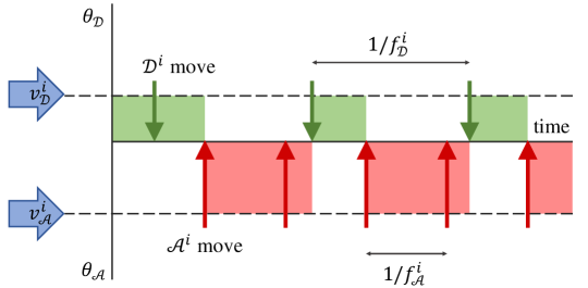
Figure 3: In each FlipIt game, $\mathcal{A}^{i}$ and $\mathcal{D}^{i}$ periodically claim control of cloud service $i.$ The values of the service for each player are given by $v_{\mathcal{A}}^{i}$ and $v_{\mathcal{D}}^{i},$ which depend on the equilibrium of the signaling game.

III-B1 Signaling Game Types

The types of each cloud service $i\in\mathbb{S}$ are $\theta^{i}\in\Theta=\left\{\theta_{\mathcal{A}},\theta_{\mathcal{D}}\right\},$ where $\theta^{i}=\theta_{\mathcal{A}}$ indicates that the service is compromised by $\mathcal{A}^{i}$, and $\theta=\theta_{\mathcal{D}}$ indicates that the service is controlled by $\mathcal{D}^{i}$. Denote the vector of all the service types by $\theta=\left[\theta^{i}\right]_{i\in\mathbb{S}}\triangleq\left[\begin{array}[]{cccc}\theta^{1}&\theta^{2}&\ldots&\theta^{m}\end{array}\right]^{T}.$

III-B2 Signaling Game Messages

Denote the risk level of the data from each service $i$ by $m^{i}\in M=\left\{m_{L},m_{H}\right\},$ where $m_{L}$ and $m_{H}$ indicate low-risk and high-risk messages, respectively. (We define this risk level in Section III-C.) Further, define the vector of all of the risk levels by $m=\left[m^{i}\right]_{i\in\mathbb{S}}.$

Next, define mixed strategies for $\mathcal{A}^{i}$ and $\mathcal{D}^{i}.$ Let $\sigma_{\mathcal{A}}^{i}:\,M\to\left[0,1\right]$ and $\sigma_{\mathcal{D}}^{i}:\,M\to\left[0,1\right]$ be functions such that $\sigma_{\mathcal{A}}^{i}\left(m_{\mathcal{A}}^{i}\right)\in\Sigma_{\mathcal{A}}$ and $\sigma_{\mathcal{D}}^{i}\left(m_{\mathcal{D}}^{i}\right)\in\Sigma_{\mathcal{D}}$ give the proportions with which $\mathcal{A}^{i}$ and $\mathcal{D}^{i}$ send messages with risk levels $m_{\mathcal{A}}^{i}$ and $m_{\mathcal{D}}^{i},$ respectively, from each cloud service $i$ that they control. Note that $\mathcal{R}$ only observes $m_{\mathcal{A}}^{i}$ or $m_{\mathcal{D}}^{i},$ depending on who controls the service $i.$ Let

$$m^{i}=\begin{cases}m_{\mathcal{A}}^{i},\quad\text{if}&\theta^{i}=\theta_{\mathcal{A}}\\ m_{\mathcal{D}}^{i},\quad\text{if}&\theta^{i}=\theta_{\mathcal{D}}\end{cases},$$

denote risk level of the message that $\mathcal{R}$ actually observes. Finally, define the vector of observed risk levels by $m=\left[m^{i}\right]_{i\in\mathbb{S}}.$

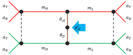
Figure 4: The vector of types $\theta\in\Theta^{N}$ defines whether each cloud service $i\in\mathbb{S}$ is controlled by an attacker or defender. Each prior probability $p_{\mathcal{A}}^{i}$ comes from the corresponding FlipIt game. The player who controls each service chooses $m^{i}.$ $\mathcal{R}$ observes all $m^{i}$ and chooses $a^{i},$ $i\in\mathbb{S}$ simultaneously. Here, we show one service, although all of the services are coupled.

III-B3 Signaling Game Beliefs and Actions

Based on the risk levels $m$ that $\mathcal{R}$ observes, it updates its vector of prior beliefs $p_{\mathcal{A}}.$ Define $\mu^{i}:\,\Theta\to\left[0,1\right],$ such that $\mu^{i}\left(\theta\,|\,m^{i}\right)$ gives the belief of $\mathcal{R}$ that service $i\in\mathbb{S}$ is of type $\theta$ given that $\mathcal{R}$ observes risk level $m^{i}.$ Also write the vector of beliefs as $\mu\left(\theta\,|\,m\right)=\left[\mu^{i}\left(\theta^{i}\,|\,m^{i}\right)\right]_{i\in\mathbb{S}}.$ As a direction for future work, we note that evidence-based signaling game approaches could be used to update belief in a manner robust to reputation attacks [29, 36, 37].

Based on these beliefs, $\mathcal{R}$ chooses which cloud services to trust. For each service $i,$ $\mathcal{R}$ chooses $a^{i}\in A=\left\{a_{T},a_{N}\right\}$ where $a_{T}$ denotes trusting the service (i.e., using it for observer-based optimal feedback control) and $a_{N}$ denotes not trusting the service. Assume that $\mathcal{R},$ aware of the system dynamics, chooses actions for each service simultaneously, i.e., $a=\left[a^{i}\right]_{i\in\mathbb{S}}.$

Next, define $\sigma_{\mathcal{R}}:\,A^{N}\to\left[0,1\right]$ such that $\sigma_{\mathcal{R}}\left(a\,|\,m\right)\in\Sigma_{\mathcal{R}}^{N}$ gives the mixed strategy probability with which $\mathcal{R}$ plays the vector of actions $a$ given the vector of risk levels $m.$

III-B4 Signaling Game Utility Functions

Let $\mathcal{R}$’s utility function be denoted by $u_{\mathcal{R}}^{S}:\,\Theta^{N}\times M^{N}\times A^{N}\to\mathbb{R},$ such that $u_{\mathcal{R}}^{S}\left(\theta,m,a\right)$ gives the utility that $\mathcal{R}$ receives when $\theta$ is the vector of cloud service types, $m$ is the vector of risk levels, and $\mathcal{R}$ chooses the vector of actions $a.$

For $i\in\mathbb{S},$ define the functions $u_{\mathcal{A}}^{S_{i}}:\,M^{N}\times A^{N}\to\mathbb{R}$ and $u_{\mathcal{D}}^{S_{i}}:\,M^{N}\times A^{N}\to\mathbb{R},$ such that $u_{\mathcal{A}}^{S_{i}}\left(m,a\right)$ and $u_{\mathcal{D}}^{S_{i}}\left(m,a\right)$ give the utility that $\mathcal{A}^{i}$ and $\mathcal{D}^{i}$ receive for service $i$ when the risk levels are given by the vector $m,$ and $\mathcal{R}$ plays the vector of actions $a.$

Next, consider expected utilities based on the strategies of each player. Let $\bar{u}_{\mathcal{R}}^{S}:\,\Sigma_{\mathcal{R}}^{N}\to\mathbb{R}$ denote the expected utility function for $\mathcal{R},$ such that $\bar{u}_{\mathcal{R}}^{S}\left(\sigma_{\mathcal{R}}\,|\,m,\mu\left(\bullet\,|\,m\right)\right)$ gives $\mathcal{R}$’s expected utility when he plays mixed strategy $\sigma_{\mathcal{R}}$ given that he observes risk levels $m$ and has belief $\mu.$ We have

$$\bar{u}_{\mathcal{R}}^{S}\left(\sigma_{\mathcal{R}}\,|\,m,\mu\right)=\underset{\theta\in\Theta^{m}}{\sum}\underset{a\in A^{m}}{\sum}u_{\mathcal{R}}^{S}\left(\theta,m,a\right)\mu\left(\theta\,|\,m\right)\sigma_{\mathcal{R}}\left(a\,|\,m\right).$$ (8)

In order to compute the expected utility functions for $\mathcal{A}^{i}$ and $\mathcal{D}^{i},$ define $\sigma_{\mathcal{A}}^{-i}=\left\{\sigma_{\mathcal{A}}^{j}\,|\,j\in\mathbb{S}\backslash\{i\}\right\}$ and $\sigma_{\mathcal{D}}^{-i}=\left\{\sigma_{\mathcal{D}}^{j}\,|\,j\in\mathbb{S}\backslash\{i\}\right\},$ the sets of the strategies of all of the senders except the sender on cloud service $i.$ Then define $\bar{u}_{\mathcal{A}}^{S_{i}}:\,\Sigma_{\mathcal{R}}^{N}\times\Sigma_{\mathcal{A}}^{N}\times\Sigma_{\mathcal{D}}^{N-1}\to\mathbb{R}$ such that $\bar{u}_{\mathcal{A}}^{S_{i}}\left(\sigma_{\mathcal{R}};\sigma_{\mathcal{A}}^{i},\sigma_{\mathcal{A}}^{-i};\sigma_{\mathcal{D}}^{-i}\right)$ gives the expected utility to $\mathcal{A}^{i}$ when he plays mixed strategy $\sigma_{\mathcal{A}}^{i},$ and the attackers and defenders on the other services play $\sigma_{\mathcal{A}}^{-i}$ and $\sigma_{\mathcal{D}}^{-i}.$ Define the expected utility to $\mathcal{D}^{i}$ by $\bar{u}_{\mathcal{D}}^{S_{i}}\left(\sigma_{\mathcal{R}};\sigma_{\mathcal{A}}^{-i};\sigma_{\mathcal{D}}^{i},\sigma_{\mathcal{D}}^{-i}\right)$ in a similar manner.

Let $\mathcal{X}^{i}\in\left\{\mathcal{A},\mathcal{D}\right\}$ denote the player that controls service $i$ and $\mathcal{X}\in\left\{\mathcal{A},\mathcal{D}\right\}^{N}$ denote the set of players that control each service. Then the expected utilities are computed by

$$\bar{u}_{\mathcal{A}}^{S_{i}}\left(\sigma_{\mathcal{R}};\sigma_{\mathcal{A}}^{i},\sigma_{\mathcal{A}}^{-i};\sigma_{\mathcal{D}}^{-i}\right)=\underset{m\in M^{N}}{\sum}\underset{a\in A^{N}}{\sum}\\ \underset{\mathcal{X}^{1}\in\left\{\mathcal{A},\mathcal{D}\right\}}{\sum}\ldots\underset{\mathcal{X}^{i-1}\in\left\{\mathcal{A},\mathcal{D}\right\}}{\sum}\underset{\mathcal{X}^{i+1}\in\left\{\mathcal{A},\mathcal{D}\right\}}{\sum}\ldots\underset{\mathcal{X}^{N}\in\left\{\mathcal{A},\mathcal{D}\right\}}{\sum}\\ u_{\mathcal{A}}^{S_{i}}\left(m,a\right)\sigma_{\mathcal{R}}\left(a\,|\,m\right)\sigma_{\mathcal{A}}^{i}\left(m^{i}\right)\underset{j\in\mathbb{S}\backslash\{i\}}{\prod}\sigma_{\mathcal{X}^{j}}^{j}\left(m^{j}\right)p_{\mathcal{X}^{j}}^{j},$$ (9)

$$\bar{u}_{\mathcal{D}}^{S_{i}}\left(\sigma_{\mathcal{R}};\sigma_{\mathcal{A}}^{-i};\sigma_{\mathcal{D}}^{i},\sigma_{\mathcal{D}}^{-i}\right)=\underset{m\in M^{N}}{\sum}\underset{a\in A^{N}}{\sum}\\ \underset{\mathcal{X}^{1}\in\left\{\mathcal{A},\mathcal{D}\right\}}{\sum}\ldots\underset{\mathcal{X}^{i-1}\in\left\{\mathcal{A},\mathcal{D}\right\}}{\sum}\underset{\mathcal{X}^{i+1}\in\left\{\mathcal{A},\mathcal{D}\right\}}{\sum}\ldots\underset{\mathcal{X}^{N}\in\left\{\mathcal{A},\mathcal{D}\right\}}{\sum}\\ u_{\mathcal{D}}^{S_{i}}\left(m,a\right)\sigma_{\mathcal{R}}\left(a\,|\,m\right)\sigma_{\mathcal{D}}^{i}\left(m^{i}\right)\underset{j\in\mathbb{S}\backslash\{i\}}{\prod}\sigma_{\mathcal{X}^{j}}^{j}\left(m^{j}\right)p_{\mathcal{X}^{j}}^{j}.$$ (10)

III-B5 Perfect Bayesian Nash Equilibrium Conditions

Finally, we can state the requirements for a perfect Bayesian Nash equilibrium (PBNE) for the signaling game [38].

Definition 2.

(PBNE) For the device, let $\bar{u}_{\mathcal{R}}^{S}\left(\sigma_{\mathcal{R}}\,|\,m,\mu\right)$ be formulated according to Eq. (8). For each service $i\in\mathbb{S},$ let $\bar{u}_{\mathcal{A}}^{S_{i}}\left(\sigma_{\mathcal{R}};\sigma_{\mathcal{A}}^{i},\sigma_{\mathcal{A}}^{-i};\sigma_{\mathcal{D}}^{-i}\right)$ be given by Eq. (9) and $\bar{u}_{\mathcal{D}}^{S_{i}}\left(\sigma_{\mathcal{R}};\sigma_{\mathcal{A}}^{-i};\sigma_{\mathcal{D}}^{i},\sigma_{\mathcal{D}}^{-i}\right)$ be given by Eq. (10). Finally, let vector $p_{\mathcal{A}}$ give the prior probabilities of each service being compromised. Then, a perfect Bayesian Nash equilibrium of the signaling game is a strategy profile $\left(\sigma_{\mathcal{R}}^{*};\sigma_{\mathcal{A}}^{1*},\ldots\sigma_{\mathcal{A}}^{N*};\sigma_{\mathcal{D}}^{1*},\ldots\sigma_{\mathcal{D}}^{N*}\right)$ and a vector of beliefs $\mu\left(\theta\,|\,m\right)$ such that the following hold:

$$\forall i\in\mathbb{S},\,\sigma_{\mathcal{A}}^{i*}\left(\bullet\right)\in\underset{\sigma_{\mathcal{A}}^{i}\in\Sigma_{\mathcal{A}}}{\arg\max\>}\bar{u}_{\mathcal{A}}^{S_{i}}\left(\sigma_{\mathcal{R}}^{*};\sigma_{\mathcal{A}}^{i},\sigma_{\mathcal{A}}^{-i*};\sigma_{\mathcal{D}}^{-i*}\right),$$ (11)

$$\forall i\in\mathbb{S},\,\sigma_{\mathcal{D}}^{i*}\left(\bullet\right)\in\underset{\sigma_{\mathcal{D}}^{i}\in\Sigma_{\mathcal{D}}}{\arg\max\>}\bar{u}_{\mathcal{D}}^{S_{i}}\left(\sigma_{\mathcal{R}}^{*};\sigma_{\mathcal{A}}^{-i*};\sigma_{\mathcal{D}}^{i},\sigma_{\mathcal{D}}^{-i*}\right),$$ (12)

$$\forall m\in M,\>\sigma_{\mathcal{R}}^{*}\in\underset{\sigma_{\mathcal{R}}\in\Sigma_{\mathcal{R}}^{m}}{\arg\max\>}\bar{u}_{\mathcal{R}}^{S}\left(\sigma_{\mathcal{R}}\,|\,m,\mu\left(\bullet\,|\,m\right)\right),$$ (13)

and $\forall i\in\mathbb{S},$

$$\mu^{i}\left(\theta_{\mathcal{A}}\,|\,m^{i}\right)=\frac{\sigma_{\mathcal{A}}^{i*}\left(m^{i}\right)p_{\mathcal{A}}^{i}}{\sigma_{\mathcal{A}}^{i*}\left(m^{i}\right)p_{\mathcal{A}}^{i}+\sigma_{\mathcal{D}}^{i*}\left(m^{i}\right)\left(1-p_{\mathcal{A}}^{i}\right)},$$ (14)

if $\sigma_{\mathcal{A}}^{i*}\left(m^{i}\right)p_{\mathcal{A}}^{i}+\sigma_{\mathcal{D}}^{i*}\left(m^{i}\right)p_{\mathcal{D}}^{i}\neq 0,$ and $\mu^{i}\left(\theta_{\mathcal{A}}\,|\,m^{i}\right)\in\left[0,1\right],$ if $\sigma_{\mathcal{A}}^{i*}\left(m^{i}\right)p_{\mathcal{A}}^{i}+\sigma_{\mathcal{D}}^{i*}\left(m^{i}\right)p_{\mathcal{D}}^{i}=0.$ Additionally, $\mu^{i}\left(\theta_{\mathcal{D}}\,|\,m^{i}\right)=1-\mu^{i}\left(\theta_{\mathcal{A}}\,|\,m^{i}\right)$ in both cases.

Note that we have denoted the equilibrium utilities for $\mathcal{A}^{i}$ and $\mathcal{D}^{i},$ $i\in\mathbb{S}$ by

$$v_{\mathcal{A}}^{i}=\bar{u}_{\mathcal{A}}^{S_{i}}\left(\sigma_{\mathcal{R}}^{*};\sigma_{\mathcal{A}}^{i*},\sigma_{\mathcal{A}}^{-i*};\sigma_{\mathcal{D}}^{-i*}\right),$$ (15)

$$v_{\mathcal{D}}^{i}=\bar{u}_{\mathcal{D}}^{S_{i}}\left(\sigma_{\mathcal{R}}^{*};\sigma_{\mathcal{A}}^{-i*};\sigma_{\mathcal{D}}^{i*},\sigma_{\mathcal{D}}^{-i*}\right),$$ (16)

and the vectors of those values by $v_{\mathcal{A}}=\left[v_{\mathcal{A}}^{i}\right]_{i\in\mathbb{S}},$ $v_{\mathcal{D}}=\left[v_{\mathcal{D}}^{i}\right]_{i\in\mathbb{S}}.$ We now have the complete description of the signaling game mapping Eq. (2), where $T^{S}:\,\left[0,1\right]^{N}\to\mathcal{P}(\mathbb{R}^{2N}).$ This mapping constitutes the middle layer of Fig. 2.

III-C Physical Layer: Optimal Control

The utility function $u_{\mathcal{R}}^{S}\left(\theta,m,a\right)$ is determined by the performance of the device controller as shown in Fig. 2. A block illustration of the control system is shown in Fig. 5. Note that the physical system in the diagram refers to the IoCT devices.

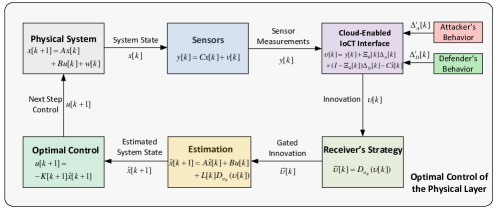
Figure 5: A block diagram shows the various components of the control system in the iSTRICT. The physical system refers to IoCT device whose states are collected by sensors. Each $\mathcal{A}^{i}$ and $\mathcal{D}^{i}$ in the cloud layer can add bias terms to the measured senor data before sending it to the receiver. $\mathcal{R}$ decides whether to trust or not trust each of the cloud services, and then designs an optimal control for the physical system. Since the optimal control is designed over a finite-horizon cost criterion, the loop terminates after $T$ time steps.

III-C1 Device Dynamics

Each device in the IoCT is governed by dynamics. We can capture the dynamics of the things by the linear system model

$$x[k+1]=Ax[k]+Bu[k]+w[k],$$ (17)

where $A\in\mathbb{R}^{n\times n}$, $B\in\mathbb{R}^{n\times q}$, $x[k]\in\mathbb{R}^{n}$ is the system state, $u[k]\in\mathbb{R}^{q}$ is the control input, $w[k]$ denotes the system white noise, and $x[0]=x_{0}\in\mathbb{R}^{n}$ is given. Let $y[k]\in\mathbb{R}^{N}$ represent data from cloud services which suffers from white, additive Gaussian sensor noise given by the vector $v[k].$ We have $y[k]=Cx[k]+v[k],$ where $C\in\mathbb{R}^{N\times n}$ is the output matrix. Let the system and sensor noise processes have known covariance matrices $\mathbb{E}\left\{w[k]w^{\prime}[k]\right\}=\xi,\;\mathbb{E}\left\{v[k]v^{\prime}[k]\right\}=\zeta,$ where $\xi$ and $\zeta$ are symmetric, positive, semi-definite matrices, and $w^{\prime}[k]$ and $v^{\prime}[k]$ denote the transposes of the noise vectors.

In addition, for each cloud service $i\in\mathbb{S},$ the attacker $\mathcal{A}^{i}$ and defender $\mathcal{D}^{i}$ in the signaling game choose whether to add bias terms to the measurement $y^{i}[k].$ Let $\Delta_{\mathcal{A}}^{i}[k],\Delta_{\mathcal{D}}^{i}[k]\in\mathbb{R}$ denote these bias terms. The actual noise levels that $\mathcal{R}$ observes depends on who controls the service in the FlipIt game. Recall that the vector of types of each service is given by $\theta=\left[\theta^{i}\right]_{i\in\mathbb{S}}.$ Let $\mathbf{1}_{\left\{\bullet\right\}}$ represent the indicator function, which takes the value of $1$ if its argument is true and $0$ otherwise. Then, define the matrix

$$\Xi_{\theta}=\text{diag}\left\{\left[\begin{array}[]{ccc}\mathbf{1}_{\left\{\theta^{1}=\theta_{\mathcal{A}}\right\}}&\ldots&\mathbf{1}_{\left\{\theta^{N}=\theta_{\mathcal{A}}\right\}}\end{array}\right]\right\}.$$

Including the bias term, the measurements are given by

$$\tilde{y}[k]=Cx[k]+v[k]+\Xi_{\theta}[k]\Delta_{\mathcal{A}}[k]+\left(I-\Xi_{\theta}[k]\right)\Delta_{\mathcal{D}}[k],$$ (18)

where $I$ is the $N$-dimensional identity matrix.

III-C2 Observer-Based Optimal Feedback Control

Let $F,$ $Q,$ and $R$ be positive-definite matrices of dimensions $n\times n,$ $n\times n,$ and $q\times q,$ respectively. The device chooses the control $u$ that minimizes the operational cost given by

$$J=\mathbb{E}\left\{x^{\prime}[T]Fx[T]+\sum_{k=0}^{T-1}x^{\prime}[k]Qx[k]+u^{\prime}[k]Ru[k]\right\},$$ (19)

subject to the dynamics of Eq. (17).

To attempt to minimize Eq. (19), the device uses observer-based optimal feedback control. Define $P[k]$ by the forward Riccati difference equation

$$P[k+1]=A\Bigl{(}P[k]-P[k]C^{\prime}\\ \left(CP[k]C^{\prime}+\xi\right)^{-1}CP[k]\Bigr{)}A^{\prime}+\zeta,$$

with $P[0]=\mathbb{E}\{(x[0]-\hat{x}[0])(x[0]-\hat{x}[0])^{\prime}\},$ and let $L[k]=P[k]C^{\prime}(CP[k]C^{\prime}+\xi)^{-1}.$ Then the observer is a Kalman filter given by [39]

$$\hat{x}[k+1]=A\hat{x}[k]+Bu[k]+L[k]\left(\tilde{y}[k]-C\hat{x}[k]\right).$$

III-C3 Innovation

In this context, the term $\tilde{y}[k]-C\hat{x}[k]$ is the innovation. Label the innovation by $\nu[k]=\tilde{y}[k]-C\hat{x}[k].$ This term is used to update the estimate $\hat{x}[k]$ of the state. We consider the components of the innovation as the signaling-game messages that the device decides whether to trust. Let us label each component of the innovation as low-risk or high-risk. For each $i\in\mathbb{S},$ we classify the innovation as

$$m^{i}=\begin{cases}m_{L},&\text{if }\left|\nu^{i}[k]\right|\leq\epsilon^{i}\\ m_{H},&\text{if }\left|\nu^{i}[k]\right|>\epsilon^{i}\end{cases},$$

where $\epsilon\in\mathbb{R}_{++}^{N}$ is a vector of thresholds. Since $\mathcal{R}$ is strategic, it chooses whether to incorporate the innovations using the signaling game strategy $\sigma_{\mathcal{R}}(a\,|\,m),$ given the vector of messages $m.$

Define a strategic innovation filter by $D_{\sigma_{\mathcal{R}}}:\,\mathbb{R}^{N}\to\mathbb{R}^{N}$ such that, given innovation $\nu,$ the components of gated innovation $\bar{\nu}=D_{\sigma_{\mathcal{R}}}(\nu)$ are given by

$$\bar{\nu}^{i}=\begin{cases}\nu^{i},&\text{if }a^{i}=a_{T}\\ 0,&\text{otherwise}\end{cases},$$

for $i\in\mathbb{S}.$ Now we incorporate the function $D_{\sigma_{\mathcal{R}}}$ into the estimator by

$$\hat{x}[k+1]=A\hat{x}[k]+Bu[k]+L[k]D_{\sigma_{\mathcal{R}}}\left(\nu[k]\right).$$

III-C4 Feedback Controller

The optimal controller is given by the feedback law $u[k]=-K[k]\hat{x}[k],$ with gain

$$K[k]=\left(B^{\prime}[k]S[K+1]B+R\right)^{-1}B^{\prime}S[k+1]A,$$

where $S[k]$ is obtained by the backward Riccati difference equation

$$S[k]=A^{\prime}\Bigl{(}S[k+1]-S[k+1]B\\ \left(B^{\prime}S[k+1]B+R\right)^{-1}B^{\prime}S[k+1]\Bigr{)}A+Q,$$

with $S[T]=F.$

III-C5 Control Criterion to Utility Mapping

The control cost $J$ determines the signaling game utility of the device $\mathcal{R}.$ This utility should be monotonically decreasing in $J.$ We consider a mapping $J\mapsto u_{\mathcal{R}}^{S}$ defined by $u_{\mathcal{R}}^{S}\left(\theta,m,a\right)=(\bar{v}_{\mathcal{R}}-\underline{v}_{\mathcal{R}})e^{-\beta_{\mathcal{R}}J}+\bar{v}_{\mathcal{R}},$ where $\bar{v}_{\mathcal{R}}$ and $\underline{v}_{\mathcal{R}}$ denote maximum and minimum values of the utility, and $\beta_{\mathcal{R}}$ represents the sensitivity of the utility to the control cost.

III-D Definition of Gestalt Nash Equilibrium

We now define the equilibrium concept for the overall game, which is called Gestalt Nash equilibrium (GNE). To differentiate with the equilibria in FlipIt game and signaling game, we use notations with a superscript $\dagger$ to emphasize the solution at GNE.

Definition 3.

(Gestalt Nash equilibrium) The triple $\left(p_{\mathcal{A}}^{\dagger},v_{\mathcal{A}}^{\dagger},v_{\mathcal{D}}^{\dagger}\right),$ where $p_{\mathcal{A}}^{\dagger}$ represents the probability of compromise of each of the cloud services, and $v_{\mathcal{A}}^{\dagger}$ and $v_{\mathcal{D}}^{\dagger}$ represent the vectors of equilibrium utilities for $\mathcal{A}^{i}$ and $\mathcal{D}^{i},$ $i\in\mathbb{S},$ constitutes a Gestalt Nash equilibrium of the overall game if both Eq. (20) and Eq. (21) are satisfied:

$$\forall i\in\left\{1,\ldots,m\right\},\;p_{\mathcal{A}}^{i\dagger}=T^{F_{i}}\left(v_{\mathcal{A}}^{i\dagger},v_{\mathcal{D}}^{i\dagger}\right),$$ (20)

$$\left(\left[\begin{array}[]{c}v_{\mathcal{A}}^{1\dagger}\\ v_{\mathcal{A}}^{2\dagger}\\ \vdots\\ v_{\mathcal{A}}^{N\dagger}\end{array}\right],\left[\begin{array}[]{c}v_{\mathcal{D}}^{1\dagger}\\ v_{\mathcal{D}}^{2\dagger}\\ \vdots\\ v_{\mathcal{D}}^{N\dagger}\end{array}\right]\right)\in T^{S}\left(\left[\begin{array}[]{c}p_{\mathcal{A}}^{1\dagger}\\ p_{\mathcal{A}}^{2\dagger}\\ \vdots\\ p_{\mathcal{A}}^{N\dagger}\end{array}\right]\right).$$ (21)

According to Definition 3, the overall game is at equilibrium when, simultaneously, each of the FlipIt games is at equilibrium and the one signaling game is at equilibrium.

IV Equilibrium Analysis

In this section, we give conditions under which a GNE exists. We start with a set of natural assumptions. Then we narrow the search for feasible equilibria. We show that the signaling game only supports pooling equilibria, and that only low-risk pooling equilibria survive selection criteria. Finally, we create a mapping that composes the signaling and FlipIt game models. We show that this mapping has a closed graph, and we use Kakutani’s fixed-point theorem to prove the existence of a GNE. In order to avoid obstructing the flow of the paper, we briefly summarize the proofs of each lemma, and we refer readers to the GNE derivations for a single cloud service in [25] and [40].

IV-A Assumptions

TABLE II: Assumptions

#	Assumption ($\forall i\in\mathbb{S}$)
A1	$0=u_{\mathcal{A}}^{S_{i}}\left(m_{L},a_{N}\right)=u_{\mathcal{A}}^{S_{i}}\left(m_{H},a_{N}\right)=u_{\mathcal{D}}^{S_{i}}\left(m_{L},a_{N}\right)=u_{\mathcal{D}}^{S_{i}}\left(m_{H},a_{N}\right).$
A2	$0<u_{\mathcal{A}}^{S_{i}}\left(m_{L},a_{T}\right)<u_{\mathcal{D}}^{S_{i}}\left(m_{H},a_{T}\right)<u_{\mathcal{D}}^{S_{i}}\left(m_{L},a_{T}\right)<u_{\mathcal{A}}^{S_{i}}\left(m_{H},a_{T}\right).$
A3	$\forall\theta^{-i},m^{-i},a^{-i},\;\;$ $u_{\mathcal{R}}^{S}\left(\theta,m,\bar{a}\right)>u_{\mathcal{R}}\left(\theta,m,\tilde{a}\right),\;\;$ where $\;\;\theta^{i}=\theta_{\mathcal{A}},$ $m^{i}=m_{H},$ $\bar{a}^{-i}=\tilde{a}^{-i}=a^{-i},$ $\bar{a}^{i}=a_{N},$ and $\tilde{a}^{i}=a_{T}.$
A4	$\forall\theta^{-i},m^{-i},a^{-i},\;\;$ $u_{\mathcal{R}}^{S}\left(\theta,m,\bar{a}\right)<u_{\mathcal{R}}^{S}\left(\theta,m,\tilde{a}\right),\;\;$ where $\;\;\theta^{i}=\theta_{\mathcal{D}},$ $m^{i}=m_{L},$ $\bar{a}^{-i}=\tilde{a}^{-i}=a^{-i},$ $\bar{a}^{i}=a_{N},$ and $\tilde{a}^{i}=a_{T}.$
A5	$\forall\theta,m^{-i},a^{-i},\;\;$ $u_{\mathcal{R}}^{S}\left(\theta,\bar{m},a\right)>u_{\mathcal{R}}^{S}\left(\theta,\tilde{m},a\right),\;\;$ where $\;\;a^{i}=a_{T},$ $\bar{m}^{-i}=\tilde{m}^{-i}=m^{-i},$ $\bar{m}^{i}=m_{L},$ and $\tilde{m}^{i}=m_{H}.$

For simplicity, let the utility functions of each signaling game sender $i$ be dependent only on the messages and actions on cloud service $i.$ That is, $\forall i\in\mathbb{S},$ $u_{\mathcal{A}}^{S_{i}}\left(m,a\right)\equiv u_{\mathcal{A}}^{S_{i}}(m^{i},a^{i})$ and $u_{\mathcal{D}}^{S_{i}}\left(m,a\right)\equiv u_{\mathcal{D}}^{S_{i}}(m^{i},a^{i}).$ This can be removed, but it makes analysis more straightforward. Table II gives five additional assumptions. Assumption A1 assumes that each $\mathcal{A}^{i}$ and $\mathcal{D}^{i},$ $i\in\mathbb{S},$ get zero utility when their messages are not trusted. A2 assumes an ordering among the utility functions for the senders in the signaling game. It implies that a) $\mathcal{A}^{i}$ and $\mathcal{D}^{i}$ get positive utility when their messages are trusted; b) for trusted messages, $\mathcal{A}$ prefers $m_{H}$ to $m_{L};$ and c) for trusted messages, $\mathcal{D}$ prefers $m_{L}$ to $m_{H}.$ These assumptions are justified if the goal of the attacker is to cause damage (with a high-risk message), while the defender is able to operate under normal conditions (with a low-risk message).

Assumptions A3-A4 give natural requirements on the utility function of the device. First, the worst case utility for $\mathcal{R}$ is trusting a high-risk message from an attacker. Assume that, on every channel $i\in\mathbb{S},$ regardless of the messages and actions on the other channels, $\mathcal{R}$ prefers to play $a^{i}=a_{N}$ if $m^{i}=m_{H}$ and $\theta^{i}=\theta_{\mathcal{A}}.$ This is given by A3. Second, the best case utility for $\mathcal{R}$ is trusting a low-risk message from a defender. Assume that, on every channel $i\in\mathbb{S},$ regardless of the messages and actions on the other channels, $\mathcal{R}$ prefers to play $a^{i}=a_{T}$ if $m^{i}=m_{L}$ and $\theta^{i}=\theta_{\mathcal{D}}.$ This is given by A4. Finally, under normal operating conditions, $\mathcal{R}$ prefers trusted low-risk messages compared to trusted high risk messages from both an attacker and a defender. This is given by A5.

IV-B GNE Existence Proof

We prove the existence of a GNE using Lemmas 1-5 and Theorem 1.

IV-B1 Narrowing the Search for GNE

Lemma 1 eliminates some candidates for GNE.

Lemma 1.

(GNE Existence Regimes [40]) Every GNE $(p_{\mathcal{A}}^{\dagger},v_{\mathcal{A}}^{\dagger},v_{\mathcal{D}}^{\dagger})$ satisfies: $\forall i\in\mathbb{S},$ $v_{\mathcal{A}}^{i},v_{\mathcal{D}}^{i}>0.$

The basic idea behind the proof of Lemma 1 is that $v_{\mathcal{A}}^{i}=0$ or $v_{\mathcal{D}}^{i}=0$ cause either $\mathcal{A}^{i}$ or $\mathcal{D}^{i}$ to give up on capturing or recapturing the cloud. The cloud becomes either completely secure or completely insecure, neither of which can result in a GNE. Lemma 1 has a significant intuitive interpretation given by Remark 1.

Remark 1.

In any GNE, for all $i\in\mathbb{S},$ $\mathcal{R}$ plays $a^{i}=a_{T}$ with non-zero probability. In other words, $\mathcal{R}$ never completely ignores any cloud service.

IV-B2 Elimination of Separating Equilibria

In signaling games, equilibria in which different types of senders transmit the same message are called pooling equilibria, while equilibria in which different types of senders transmit distinct messages are called separating equilibria [38]. The distinct messages in separating equilibria completely reveal the type of the sender to the receiver. Lemma 2 is typical of signaling games between players with opposed incentives.

Lemma 2.

(No Separating Equilibria [40]) Consider all pure-strategy signaling-game equilibria $\left(\sigma_{\mathcal{R}}^{*};\sigma_{\mathcal{A}}^{1*},\ldots\sigma_{\mathcal{A}}^{N*};\sigma_{\mathcal{D}}^{1*},\ldots\sigma_{\mathcal{D}}^{N*}\right)$ in which each $\mathcal{A}^{i}$ and $\mathcal{D}^{i},$ $i\in\mathbb{S},$ receive positive expected utility. All such equilibria satisfy $\sigma_{\mathcal{A}}^{i*}(m)=\sigma_{\mathcal{D}}^{i*}(m)$ for all $m\in M$ and $i\in\mathbb{S}.$ That is, the senders on each cloud service $i$ use pooling strategies.

Lemma 2 holds because it is never incentive-compatible for an attacker $\mathcal{A}^{i}$ to reveal his type, in which case $\mathcal{R}$ would not trust $\mathcal{A}^{i}.$ Hence, $\mathcal{A}^{i}$ always imitates $\mathcal{D}^{i}$ by pooling.

IV-B3 Signaling Game Equilibrium Selection Criteria

Four pooling equilibria are possible in the signaling game: $\mathcal{A}^{i}$ and $\mathcal{D}^{i}$ transmit $m^{i}=m_{L}$ and $\mathcal{R}$ plays $a^{i}=a_{T}$ (which we label EQ-L1), $\mathcal{A}^{i}$ and $\mathcal{D}^{i}$ transmit $m^{i}=m_{L}$ and $\mathcal{R}$ plays $a^{i}=a_{N}$ (EQ-L2), $\mathcal{A}^{i}$ and $\mathcal{D}^{i}$ transmit $m^{i}=m_{H}$ and $\mathcal{R}$ plays $a^{i}=a_{T}$ (EQ-H1), and $\mathcal{A}^{i}$ and $\mathcal{D}^{i}$ transmit $m^{i}=m_{H}$ and $\mathcal{R}$ plays $a^{i}=a_{N}$ (which we label EQ-H2). In fact, the signaling game always admits multiple equilibria. Lemma 3 performs equilibrium selection.

Lemma 3.

(Selected Equilibria) The intuitive criterion [41] and the criterion of first mover advantage imply that equilibria EQ-L1 and EQ-L2 will be selected.

Proof:

The first mover advantage states that, if both $\mathcal{A}^{i}$ and $\mathcal{D}^{i}$ prefer one equilibrium over the others, they will choose the preferred equilibrium. Thus, $\mathcal{A}^{i}$ and $\mathcal{D}^{i}$ will always choose EQ-L1 or EQ-H1 if either of those is admitted. When neither is admitted, we select EQ-L2. When both are admitted, we use the intuitive criterion to select among them. Assumption A2 states that $\mathcal{A}^{i}$ prefers EQ-H1, while $\mathcal{D}^{i}$ prefers EQ-L1. Thus, if a sender deviates from EQ-H1 to EQ-L1, $\mathcal{R}$ can infer that the sender is a defender, and trust the message. Therefore, the intuitive criterion rejects EQ-H1 and selects EQ-L1. Finally, Assumption A5 can be used to show that EQ-H1 is never supported without EQ-L1. Hence, only EQ-L1 and EQ-L2 survive the selection criteria. ∎

At the boundary between the parameter regime that supports EQ-L1 and the parameter regime that supports EQ-L2, $\mathcal{R}$ can choose any mixed strategy, in which he plays both $a^{i}=a_{T}$ and $a^{i}=a_{N}$ with some probability. Indeed, for any cloud service $i\in\mathbb{S},$ hold $p_{\mathcal{A}}^{j},$ $j\neq i$ and $j\in\mathbb{S},$ constant, and let $p_{\mathcal{A}}^{i\diamond}$ denote the boundary between the EQ-L1 and EQ-L2 regions. Then Remark 2 gives an important property of $p_{\mathcal{A}}^{i\diamond}.$

Remark 2.

By Lemma 1, all GNE satisfy $p_{\mathcal{A}}^{i}\leq p_{\mathcal{A}}^{i\diamond}.$ Therefore, $p_{\mathcal{A}}^{i\diamond}$ is a worst-case probability of compromise.

Remark 2 is a result of the combination of the signaling and FlipIt games. Intuitively, it states that strategic trust in the communication layer is able to limit the probability of compromise of a cloud service, regardless of the attack and defense costs in the cyber layer.

IV-B4 FlipIt Game Properties

For the FlipIt games on each cloud service $i\in\mathbb{S},$ denote the ratio of attacker and defender expected utilities by $v_{\mathcal{AD}}^{i}=v_{\mathcal{A}}^{i}/v_{\mathcal{D}}^{i}.$ For $i\in\mathbb{S},$ define the set $\mathbb{V}^{i}$ by

$$\mathbb{V}^{i}=\left\{v\in\mathbb{R}_{+}\,:\,0\leq v\leq u_{\mathcal{A}}^{S_{i}}(m_{L},a_{T})/u_{\mathcal{D}}^{S_{i}}(m_{L},a_{T})\right\}.$$

Also define the set $\mathbb{PR}^{i},$ $i\in\mathbb{S},$ by $\mathbb{PR}^{i}=$

$$\left\{p\in[0,1]\,:\,0<p<T^{F_{i}}\left(u_{\mathcal{A}}^{S_{i}}(m_{L},a_{T}),u_{\mathcal{D}}^{S_{i}}(m_{L},a_{T})\right)\right\}.$$

Next, for $i\in\mathbb{S},$ define modified FlipIt game mappings $\tilde{T}^{F_{i}}:\,\mathbb{V}^{i}\to\mathbb{PR}^{i},$ where

$$p_{\mathcal{A}}^{i*}=\tilde{T}^{F_{i}}\left(v_{\mathcal{AD}}^{i}\right)\iff p_{\mathcal{A}}^{i*}\in T^{F_{i}}\left(v_{\mathcal{A}}^{i},v_{\mathcal{D}}^{i}\right).$$ (22)

Then Lemma 4 holds.

Lemma 4.

(Continuity of $\tilde{T}^{F_{i}}$ [25]) For $i\in\mathbb{S},$ $\tilde{T}^{F_{i}}(v_{\mathcal{AD}}^{i})$ is continuous in $v_{\mathcal{AD}}^{i}\in\mathbb{V}^{i}.$

The dashed curve in Fig. 6 gives an example of $\tilde{T}^{F_{i}}$ for $i=1.$ The independent variable is on the vertical axis, and the dependent variable is on the horizontal axis.

IV-B5 Signaling Game Properties

Let $v_{\mathcal{AD}}=[v_{\mathcal{AD}}^{i}]_{i\in\mathbb{S}},$ $\mathbb{V}=\prod_{i\in\mathbb{S}}\mathbb{V}^{i},$ and $\mathbb{PR}=\prod_{i\in\mathbb{S}}\mathbb{PR}^{i}.$ Define a modified signaling game mapping by $\tilde{T}^{S}:\,\mathbb{PR}\to\mathcal{P}(\mathbb{V})$ such that

$$v_{\mathcal{AD}}^{*}\in\tilde{T}^{S}\left(p_{\mathcal{A}}\right)\iff\left(v_{\mathcal{A}}^{*},v_{\mathcal{D}}^{*}\right)\in T^{S}\left(p_{\mathcal{A}}\right),$$ (23)

where $T^{S}$ selects the equilibria given by Lemma 3. Then we have Lemma 5.

Lemma 5.

(Properties of $\tilde{T}^{S}$) Construct a graph

$$\mathbb{G}=\left\{\left(p_{\mathcal{A}},v_{\mathcal{AD}}^{*}\right)\in\mathbb{PR}\times\mathbb{V}\,:\,v_{\mathcal{AD}}^{*}\in\tilde{T}^{S}\left(p_{\mathcal{A}}\right)\right\},$$

The graph $\mathbb{G}$ is closed. Additionally, for every $p_{\mathcal{A}}\in\mathbb{PR},$ the set of outputs of $\tilde{T}^{S}(p_{\mathcal{A}})$ is non-empty and convex.

Proof:

The graph $\mathbb{G}$ is closed because it contains all of its limit points. The set of outputs is non-empty because a signaling game equilibrium exists for all $p_{\mathcal{A}}.$ It is convex because expected utilities for mixed-strategy equilibria are convex combinations of pure strategy utilities and because assumption A2 implies that convexity also holds for the ratio of the utilities. ∎

The step functions (plotted with solid lines) in Figure 6 plot example mappings from $p_{\mathcal{A}}^{1}$ on the horizontal axis to $v_{\mathcal{AD}}^{1}$ on the vertical axis for $v_{\mathcal{AD}}\in\tilde{T}^{S}(p_{\mathcal{A}}),$ holding $p_{\mathcal{A}}^{i},$ $i\in\{2,3,\ldots,N\}$ fixed. It is clear that the graphs are closed.

IV-B6 Fixed-Point Theorem

By combining Eq. (20-21) with Eq. (22) and Eq. (23), we see that the vector of equilibrium utility ratios $v_{\mathcal{AD}}^{\dagger}=[v_{\mathcal{AD}}^{i\dagger}]_{i\in\mathbb{S}}$ in any GNE $(p_{\mathcal{A}}^{\dagger},v_{\mathcal{A}}^{\dagger},v_{\mathcal{D}}^{\dagger})$ must satisfy

$$\left[\begin{array}[]{c}v_{\mathcal{AD}}^{1\dagger}\\ v_{\mathcal{AD}}^{2\dagger}\\ \vdots\\ v_{\mathcal{AD}}^{N\dagger}\end{array}\right]\in\tilde{T}^{S}\left(\left[\begin{array}[]{c}\tilde{T}^{F_{1}}\left(v_{\mathcal{AD}}^{1\dagger}\right)\\ \tilde{T}^{F_{2}}\left(v_{\mathcal{AD}}^{2\dagger}\right)\\ \vdots\\ \tilde{T}^{F_{2}}\left(v_{\mathcal{AD}}^{N\dagger}\right)\end{array}\right]\right).$$

Denote this composed mapping by $\tilde{T}^{S\circ F}:\,\mathbb{V}\to\mathcal{P}(\mathbb{V})$ such that the GNE requirement can be written by $v_{\mathcal{AD}}^{\dagger}\in\tilde{T}^{S\circ F}(v_{\mathcal{AD}}^{\dagger}).$ Figure 6 gives a one-dimensional intuition behind Theorem 2. The example signaling game step functions $\tilde{T}^{S}$ have closed graphs, and the outputs of the functions are non-empty and convex. The FlipIt curve $\tilde{T}^{F_{1}}$ is continuous. The two mappings are guaranteed to intersect, and the intersection is a GNE.

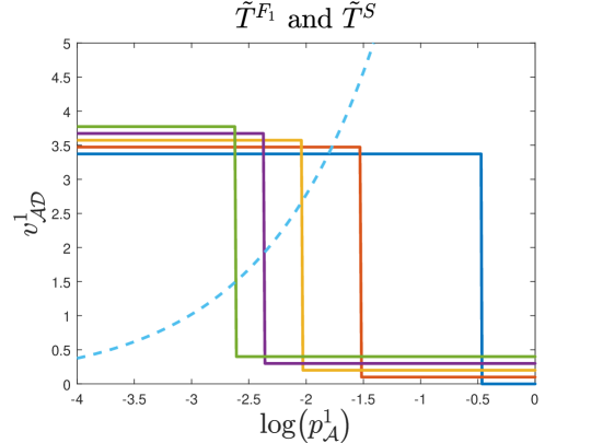
Figure 6: The (solid) step-functions depict modified signaling game mappings $\tilde{T}^{S}$ for five different sets of parameters. The (dashed) curve depicts a modified FlipIt game mapping $\tilde{T}^{F_{1}}.$ The intersection is a GNE. The figure shows only one dimension out of $N$ dimensions.

According to Lemma 5, the graph $\mathbb{G}$ of the signaling game mapping is closed, and the set of outputs of $\tilde{T}^{S}$ is non-empty and convex. Since each modified FlipIt game mapping $\tilde{T}^{F_{i}},$ $i\in\mathbb{S}$ is a continuous function, each $\tilde{T}^{F_{i}}$ produces a closed graph and has non-empty and (trivially) convex outputs. Thus, the graph of the composed mapping, $\tilde{T}^{S\circ F},$ is also closed, and has non-empty and convex outputs. Because of this, we can apply Kakutani’s fixed-point theorem, famous for its use in proving Nash equilibrium.

Theorem 1.

(Kakutani Fixed-Point Theorem [42]) - Let $\Phi$ be a non-empty, compact, and convex subset of some Euclidean space $\mathbb{R}^{n}.$ Let $Z:\,\Phi\to\mathcal{P}(\Phi)$ be a set-valued function on $\Phi$ with a closed graph and the property that, for all $\phi\in\Phi,$ $Z(\phi)$ is non-empty and convex. Then $Z$ has a fixed point.

The mapping $\tilde{T}^{S\circ F}$ is a set-valued function on $\mathbb{V},$ which is a non-empty, compact, and convex subset of $\mathbb{R}^{N}.$ $\tilde{T}^{S\circ F}$ also has a closed graph, and the set of its outputs is non-empty and convex. Therefore, $\tilde{T}^{S\circ F}$ has a fixed-point, which is precisely the definition of a GNE. Hence, we have Theorem 2.

Theorem 2.

(GNE Existence) Let the utility functions in the signaling game satisfy Assumptions A1-A5. Then a GNE exists.

Proof:

The proof has been constructed from Lemmas 1-5 and Theorem 1. ∎

Algorithm 1 Adaptive defense algorithm for iSTRICT

1. Initialize parameters $\alpha_{\mathcal{A}}^{i}$, $\alpha_{\mathcal{D}}^{i}$, $p_{\mathcal{A}}^{i}$, $p_{\mathcal{D}}^{i}$, $\forall i\in\mathbb{S}$, in each FlipIt game, and $\sigma_{\mathcal{A}}^{{i}}$ and $\sigma_{\mathcal{D}}^{{i}}$, $\forall i\in\mathbb{S}$, $\sigma_{\mathcal{R}}$ in the signaling game
   Signaling game:

2. Solve optimization problems in Eq. (11) and Eq. (12), respectively, and obtain $\sigma_{\mathcal{A}}^{{i}*}$ and $\sigma_{\mathcal{D}}^{{i}*}$, $\forall i\in\mathbb{S}$

3. Update belief $\mu^{i}(\theta_{\mathcal{A}}\,|\,m^{i})$ based on Eq. (14), and $\mu^{i}(\theta_{\mathcal{D}}\,|\,m^{i})=1-\mu^{i}(\theta_{\mathcal{A}}\,|\,m^{i})$, $\forall i\in\mathbb{S}$

4. Solve receiver’s problem in Eq. (13) and obtain $\sigma_{\mathcal{R}}^{*}$

5. If $\sigma_{\mathcal{A}}^{{i}*},\sigma_{\mathcal{D}}^{{i}*},\sigma_{\mathcal{R}}^{*}$ do not change, go to step 6; otherwise, go back to step 2

6. Obtain $v_{\mathcal{A}}^{i}$ and $v_{\mathcal{D}}^{i}$, $\forall i\in\mathbb{S}$, from Eq. (15) and Eq. (16), respectively
   FlipIt game:

7. Solve defenders’ and attackers’ problems in Eq. (6) and Eq. (7) jointly, and obtain $f_{\mathcal{A}}^{i*}$ and $f_{\mathcal{D}}^{i*}$, $\forall i\in\mathbb{S}$

8. Map the frequency pair $(f_{\mathcal{A}}^{i*},f_{\mathcal{D}}^{i*})$ to the probability pair $(p_{\mathcal{A}}^{i*},p_{\mathcal{D}}^{i*})$ through Eq. (3), $\forall i\in\mathbb{S}$

9. If $(p_{\mathcal{D}}^{i*},p_{\mathcal{A}}^{i*})$, $\forall i\in\mathbb{S}$, do not change, go to step 10; otherwise, go back to step 2

10. Return $p_{\mathcal{A}}^{\dagger}\coloneqq p_{\mathcal{A}}^{*}$, $\sigma_{\mathcal{A}}^{{i}\dagger}\coloneqq\sigma_{\mathcal{A}}^{{i}*}$, $\sigma_{\mathcal{D}}^{{i}\dagger}\coloneqq\sigma_{\mathcal{D}}^{{i}*}$, $\forall i\in\mathbb{S},$ and $\sigma_{\mathcal{R}}^{\dagger}\coloneqq\sigma_{\mathcal{R}}^{*}$

IV-C Adaptive Algorithm

Numerical simulations suggest that Assumptions A1-A5 often hold. If this is not the case, however, Algorithm 1 can be used to compute the GNE. The main idea of the adaptive algorithm is to update the strategic decision-making of different entities in iSTRICT iteratively.

Given the probability vector $p_{\mathcal{A}},$ Lines 2-5 of Algorithm 1 compute a PBNE for the signaling game which consists of the strategy profile $\left(\sigma_{\mathcal{R}}^{*};\sigma_{\mathcal{A}}^{1*},\ldots\sigma_{\mathcal{A}}^{N*};\sigma_{\mathcal{D}}^{1*},\ldots\sigma_{\mathcal{D}}^{N*}\right)$ and belief vector $\mu\left(\theta\,|\,m\right).$ The algorithm computes the PBNE iteratively using best response. The vectors of equilibrium utilities $\left(v_{\mathcal{A}}^{*},v_{\mathcal{D}}^{*}\right)$ are given by Eq. (15) and Eq. (16). Using $\left(v_{\mathcal{A}}^{*},v_{\mathcal{D}}^{*}\right),$ Line 7 of Algorithm 1 updates the equilibrium strategies of the FlipIt games and arrives at a new prior probability pair $(p_{\mathcal{A}}^{i*},p_{\mathcal{D}}^{i*}),$ $\forall i\in\mathbb{S},$ through the mapping in Eq. (3). This initializes the next round of the signaling game with the new $(p_{\mathcal{A}}^{i*},p_{\mathcal{D}}^{i*}).$ The algorithm terminates when the probabilities remain unchanged between rounds.

To illustrate Algorithm 1, we next present an example including $N=4$ cloud services. The detailed physical meaning of each service will be presented in Section V. Specifically, the costs of renewing control of cloud services are $\alpha_{\mathcal{A}}^{1}=\$2$k, $\alpha_{\mathcal{A}}^{2}=\$0.8$k, $\alpha_{\mathcal{A}}^{3}=\$10$k, $\alpha_{\mathcal{A}}^{4}=\$12$k, and $\alpha_{\mathcal{D}}^{1}=\$0.2$k, $\alpha_{\mathcal{D}}^{1}=\$0.1$k, $\alpha_{\mathcal{D}}^{1}=\$0.05$k, $\alpha_{\mathcal{D}}^{1}=\$0.03$k, for the attackers and defenders, respectively. The initial proportions of time of each attacker and defender controlling the cloud services are $p_{\mathcal{A}}^{1}=0.2$, $p_{\mathcal{A}}^{2}=0.4$, $p_{\mathcal{A}}^{3}=0.6$, $p_{\mathcal{A}}^{4}=0.15$, and $p_{\mathcal{D}}^{1}=0.8$, $p_{\mathcal{D}}^{2}=0.6$, $p_{\mathcal{D}}^{3}=0.4$, $p_{\mathcal{D}}^{4}=0.85$, respectively. For the signaling game at the communication layer, the initial probabilities that attacker sends low-risk message at each cloud service are equal to 0.2, 0.3, 0.1, and 0.4, respectively. Similarly, the defender’s initial probabilities of sending low-risk message are equal to 0.9, 0.8, 0.95, and 0.97, respectively. Figure 7 presents the results of Algorithm 1 on this example system. The result in Fig. 7a shows that the cloud services 1 and 2 can be compromised by the attacker. Figure. 7a shows the device’s belief on the received information. At the GNE, the attacker also sends low-risk message to deceive the receiver and gain utility when controlling the cloud service. Four representative devices’ actions are shown in Fig. 7b, where the devices strategically reject low-risk message in some cases due to the couplings between layers in iSTRICT. Because of the large attack and defense cost ratios and the crucial impact on physical system performance of services 3 and 4, $p_{\mathcal{D}}^{3}=p_{\mathcal{D}}^{4}=1$, insuring a secure information provision. In addition, the defense strategies at the cloud layer and the communication layer are adjusted adaptively according to the attackers’ behaviors. Within each layer, all players are required to best respond to the strategies of the other players. This cross-layer approach enables a defense-in-depth mechanism for the devices in iSTRICT.

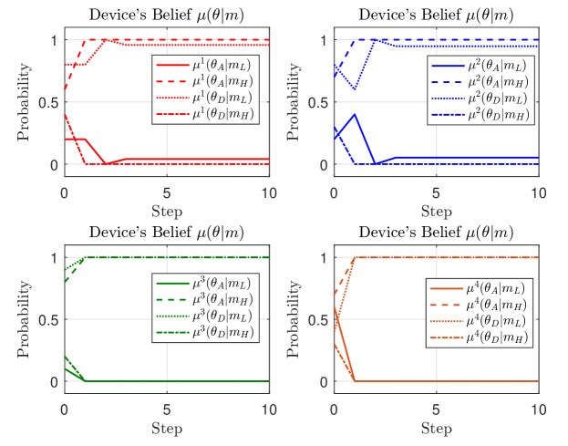
(a) Device belief

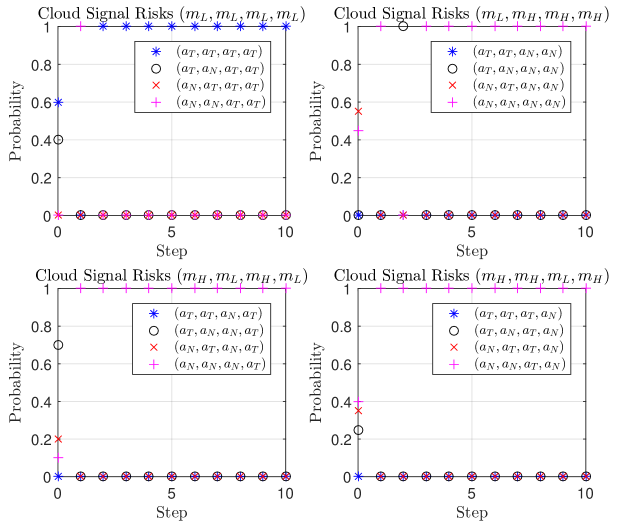
(b) Device action

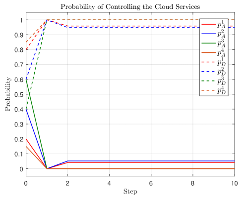
(c) FlipIt game

Figure 7: Adaptive Algorithm with four cloud services. (a) and (b) depict each device’s belief and action, respectively. (c) shows the result of cloud security. The algorithm converges to a GNE in four steps, where one step represents a round of updates including the FlipIt game and signaling game.

V Application to Autonomous Vehicle Control

In this section, we apply iSTRICT to a cloud-enabled autonomous vehicle network in which the framework of vehicular cloud computing is similar to the one in [43]. Two autonomous vehicles use an observer to estimate their positions and velocities based on measurements from six sources, four of which may be compromised. They also implement optimal feedback control based on the estimated state.

V-A Autonomous Vehicle Security

Autonomous vehicle technology will make a powerful impact on several industries. In the automotive industry, traditional car companies as well as technology firms such as Google [44] are racing to develop autonomous vehicle technology. Maritime shipping is also an attractive application of autonomous vehicles. Autonomous ships are expected to be safer, higher-capacity, and more resistant to piracy attacks [45]. Finally, unmanned aerial vehicles (UAVs) have the potential to reshape fields such as mining, disaster relief, and precision agriculture [46].

Nevertheless, autonomous vehicles pose clear safety risks. In ground transportation, in March of 2018, an Uber self-driving automobile struck and killed a pedestrian [47]. On the sea, multiple crashes of ships in the Unites States Navy during 2017 [48] have prompted concerns about too much reliance on automation. In the air, cloud-enabled UAVs could be subject to data integrity or availability attacks [49]. In general, autonomous vehicles rely on many remote sources (e.g., other vehicles, GPS signals, location-based services) for information. In the most basic case, these sources are subject to errors that must be handled robustly. In addition, the sources could also be selfish and strategic. For instance, an autonomous ship could transmit its own coordinates dishonestly in order to clear its own shipping path of other vessels. In the worst case, the sources could be malicious. An attacker could use a spoofed GPS signal in order to destroy a UAV or to use the UAV to attack another target. In all of these cases, autonomous vehicles must decide whether to trust the remote sources of information.

V-B Physical-Layer Implementation

We consider an interaction between nine agents. Two autonomous vehicles implement observer-based optimal feedback control according to the iSTRICT framework. Each vehicle has two states: position and angle. Thus, the combined system has the state vector $x[k]\in\mathbb{R}^{4}$ described in Fig. 8. The states evolve over finite horizon $k\in\{0,1,\ldots,T\}.$

These states are observed through both remote and local measurements. Figure 9 describes these measurements. The local measurements $y^{5}[k]$ and $y^{6}[k]$ originate from sensors on the autonomous vehicle, so these are secure. Hence, the autonomous vehicle always trusts $y^{5}[k]$ and $y^{6}[k].$ In addition, while the magnetic compass sensors are subject to electromagnetic attack, this involves high attack costs $\alpha_{\mathcal{A}}^{3}$ and $\alpha_{\mathcal{A}}^{4}$. The defense algorithm yields that $\mathcal{R}$ always trusts $y^{3}[k]$ and $y^{4}[k]$ at the GNE. The remote measurements $\tilde{y}^{1}[k]$ and $\tilde{y}^{2}[k]$ are received from cloud services that may be controlled by defenders $\mathcal{D}^{1}$ and $\mathcal{D}^{2},$ or that may be compromised by attackers $\mathcal{A}^{1}$ and $\mathcal{A}^{2}.$

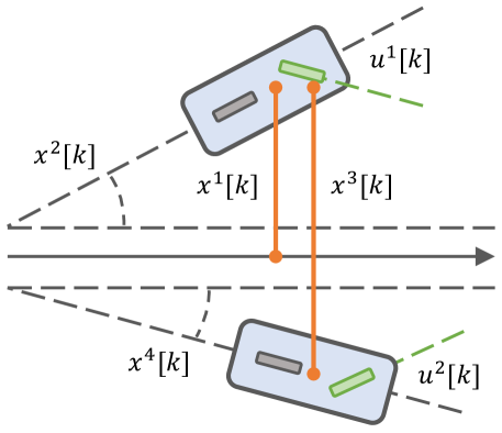
Figure 8: We use bicycle steering models from [50] to conceptually capture the vehicle dynamics. The vehicle states are given by $x^{1}[k]:$ first vehicle position, $x^{2}[k]:$ first vehicle angle; $x^{3}[k]:$ offset between vehicles; $x^{4}[k]:$ second vehicle angle. Controls $u^{1}[k]$ and $u^{2}[k]$ represent the steering angles of the first and second vehicles, respectively.

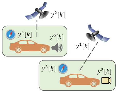
Figure 9: Local sensors include a localization camera on vehicle 1 and a range finding device on vehicle 2. Remote sensors include magnetic compass sensors and GPS receivers on both vehicles.

In the signaling game, attackers $\mathcal{A}^{1}$ and $\mathcal{A}^{2}$ may add bias terms $\Delta_{\mathcal{A}}^{1}[k]$ or $\Delta_{\mathcal{A}}^{2}[k]$ if $\theta^{1}=\theta_{\mathcal{A}}$ or $\theta^{2}=\theta_{\mathcal{A}},$ respectively. Therefore, the autonomous vehicles must strategically decide whether to trust these measurements. Each $\tilde{y}^{i}[k],$ $i\in\{1,2\},$ is classified as a low-risk ($m^{i}=m_{L})$ or high-risk ($m^{i}=m_{H})$ message according to an innovation filter. $\mathcal{R}$ decides whether to trust each message according to the action vector $a=[\begin{array}[]{cc}a^{1}&a^{2}\end{array}]^{\prime},$ where $a^{1},a^{2}\in\{a_{N},a_{T}\}.$ We seek an equilibrium of the signaling game that satisfies Definition 2.

V-C Signaling Game Results

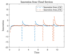
(a) Innovation

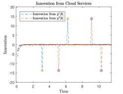
(b) Innovation

(c) Innovation

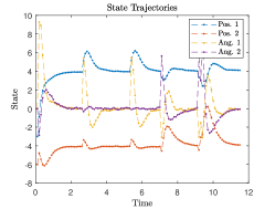
(d) State trajectories

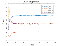
(e) State trajectories

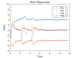
(f) State trajectories

Figure 10: Column 1: $\mathcal{A}^{1}$ and $\mathcal{A}^{2}$ send $m_{H}$ and $\mathcal{R}$ plays $[\begin{array}[]{cc}a_{T}&a_{T}\end{array}]^{\prime},$ Column 2: $\mathcal{A}^{1}$ and $\mathcal{A}^{2}$ send $m_{H}$ and $\mathcal{R}$ plays $[\begin{array}[]{cc}a_{N}&a_{N}\end{array}]^{\prime},$ Column 3: $\mathcal{A}^{1}$ and $\mathcal{A}^{2}$ send $m_{L}$ and $\mathcal{R}$ plays $[\begin{array}[]{cc}a_{T}&a_{T}\end{array}]^{\prime}.$ Row 1: Innovation, Row 2: State trajectories.

Figure 10 depicts the results of three different signaling-game strategy profiles for the attackers, defenders, and device, using the software MATLAB [51]. The observer and controller are linear, so the computation is rapid. Each iteration of the computational elements of the control loop depicted in Fig. 5 takes less than 0.0002s on a Lenovo ThinkPad L560 laptop with 2.30 GHz processor and 8.0 GB of installed RAM.

In all of the scenarios, we set the position of the first vehicle to a track a reference trajectory of $x^{1}[k]=4,$ the offset between the second vehicle and the first vehicle to track a reference trajectory of $x^{3}[k]=8,$ and both angles to target $x^{2}[k]=x^{4}[k]=0.$ Column 1 depicts a scenario in which $\mathcal{A}^{1}$ and $\mathcal{A}^{2}$ send $m_{H}$ and $\mathcal{R}$ plays $a^{1}=a^{2}=a_{T}.$ The spikes in the innovation represent the bias terms added by the attacker when he controls the cloud. The spikes in Fig. 10(a) are large because these the attacker adds bias terms corresponding to high risk messages. These bias terms cause large deviations in the position and angle from their desired values (Fig. 10(d)). For instance, at time $10,$ the two vehicles come within approximately $4$ units of each other.

Column 2 depicts the best response of $\mathcal{R}$ to this strategy. The vehicle uses an innovation filter (here, at $\epsilon^{1}=\epsilon^{2}=10$) which categorizes the biased innovations as $m_{H}.$ The best response is to choose

$$\sigma_{\mathcal{R}}\left(\left[\begin{array}[]{c}a_{T}\\ a_{T}\end{array}\right]|\left[\begin{array}[]{c}m_{L}\\ m_{L}\end{array}\right]\right)=\sigma_{\mathcal{R}}\left(\left[\begin{array}[]{c}a_{T}\\ a_{N}\end{array}\right]|\left[\begin{array}[]{c}m_{L}\\ m_{H}\end{array}\right]\right)=1,$$

$$\sigma_{\mathcal{R}}\left(\left[\begin{array}[]{c}a_{N}\\ a_{T}\end{array}\right]|\left[\begin{array}[]{c}m_{H}\\ m_{L}\end{array}\right]\right)=\sigma_{\mathcal{R}}\left(\left[\begin{array}[]{c}a_{N}\\ a_{N}\end{array}\right]|\left[\begin{array}[]{c}m_{H}\\ m_{H}\end{array}\right]\right)=1,$$

i.e., to trust only low-risk messages. The circled data points in Fig. 10(b) denote high-risk innovations from the attacker that are rejected. Figure 10(e) shows that this produces very good results in which the positions of the first and second vehicle converge to their desired values of $4$ and $-4,$ respectively, and the angles converge to $0.$

But iSTRICT assumes that the attackers are also strategic. $\mathcal{A}^{1}$ and $\mathcal{A}^{2}$ realize that high-risk messages will be rejected, so they add smaller bias terms $\Delta_{\mathcal{A}}^{1}[k]$ and $\Delta_{\mathcal{A}}^{2}[k]$ which are classified as $m_{L}.$ This is depicted by Fig. 10(c). It is not optimal for the autonomous vehicle to reject all low-risk messages, because most such messages come from a cloud controlled by the defender. Therefore, the device must play $a^{1}=a^{2}=a_{T}.$ Nevertheless, Fig. 10(f) shows that these low-risk messages create significantly less disturbance than the disturbances from high-risk messages in Fig. 10(d). In summary, the signaling-game equilibrium is for $\mathcal{A}^{1},$ $\mathcal{A}^{2},$ $\mathcal{D}^{1},$ and $\mathcal{D}^{2}$ to transmit low-risk messages and for $\mathcal{R}$ to trust low-risk messages while rejecting high-risk messages off the equlibrium path.

V-D Results of the FlipIt Games

Meanwhile, $\mathcal{A}^{1}$ and $\mathcal{D}^{1}$ play a FlipIt game for control of Cloud Service 1, and $\mathcal{A}^{2}$ and $\mathcal{D}^{2}$ play a FlipIt game for control of Cloud Service 2. Based on the equilibrium of the signaling game, all players realize that the winners of the FlipIt games will be able to send trusted low-risk messages, but not trusted high-risk messages. Based on Assumption A2, low-risk messages are more beneficial to the defenders than to the attackers. Hence, the incentives to control the cloud are larger for defenders than for attackers. This results in a low $p_{\mathcal{A}}^{1}$ and $p_{\mathcal{A}}^{2}$ from the FlipIt game. If the equilibrium from the previous subsection holds for these prior probabilities, then the overall five-player interaction is at a GNE as described in Definition 3 and Theorem 2.

Table III is useful for benchmarking the performance of iSTRICT. The table lists the empirical value of the control criterion given by Eq. (19). The first three columns quantify the performance depicted in Fig. 10. Column $1$ is the benchmark case, in which $\mathcal{A}^{1}$ and $\mathcal{A}^{2}$ add high-risk noise, and the noise is mitigated somewhat by a Kalman filter, but the bias is not handled optimally. Column 2 shows the improvement provided by iSTRICT against a nonstrategic attacker, and Column 3 shows the improvement provided by iSTRICT against a strategic attacker. The improvement is largest in Column 2, but it is significant against a strategic attacker as well.

TABLE III: Control Costs and Benchmarks for the Simulations depicted in Fig. 11-12

	Ungated $m_{H}$	Gated $m_{H}$	Trusted $m_{L}$	Trusted, Frequent $m_{L}$	Untrusted, Frequent $m_{L}$	Mixed Trust with $m_{L}$
Trial 1	274,690	42,088	116,940	185,000	128,060	146,490
Trial 2	425,520	42,517	123,610	211,700	121,910	143,720
Trial 3	119,970	42,444	125,480	213,500	144,090	130,460
Trial 4	196,100	42,910	89,980	239,400	138,350	135,930
Trial 5	229,870	42,733	66,440	94,400	135,160	139,680
Trial 6	139,880	42,412	69,510	2,581,500	119,700	125,270
Trial 7	129,980	42,642	116,560	254,000	138,160	122,790
Trial 8	97,460	42,468	96,520	1,020,000	130,260	146,370
Trial 9	125,490	42,633	50,740	250,900	138,960	151,470
Trial 10	175,670	42,466	78,700	4,182,600	135,780	126,550
Average	191,463	42,531	93,448	923,300	133,043	136,873

V-E GNE for Different Parameters

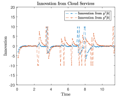
(a) Innovation

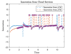
(b) Innovation

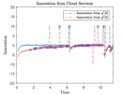
(c) Innovation

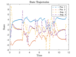
(d) State trajectories

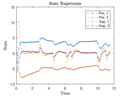
(e) State trajectories

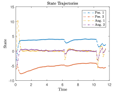
(f) FlipIt game

Figure 11: Column 1: Innovation and state trajectories for $p_{\mathcal{A}}^{2}=0.10$ and $\mathcal{R}$ plays $[\begin{array}[]{cc}a_{T}&a_{T}\end{array}]^{\prime},$ Column 2: Innovation and state trajectories for $p_{\mathcal{A}}^{2}=0.10$ and $\mathcal{R}$ plays $[\begin{array}[]{cc}a_{T}&a_{N}\end{array}]^{\prime},$ Column 3: Innovation and state trajectories in which $\mathcal{R}$ mixes strategies between $[\begin{array}[]{cc}a_{T}&a_{T}\end{array}]^{\prime}$ and $[\begin{array}[]{cc}a_{T}&a_{N}\end{array}]^{\prime}.$

Now consider a parameter change in which $\mathcal{A}^{2}$ develops new malware to compromise the GPS position signal $\tilde{y}^{2}[k]$ at a much lower cost $\alpha_{\mathcal{A}}^{2}.$ (See Subsection III-A). In equilibrium, this increases $p_{\mathcal{A}}^{2}$ from $0.03$ to $0.10.$ A higher number of perturbed innovations are visible in Fig. 11(a). This leads to the poor state trajectories of Fig. 11(d). The control cost from Eq. (19) increases, and the two vehicles nearly collide at time $8.$ The large changes in angles show that the vehicles turn rapidly in different directions.

In this case, $\mathcal{R}$’s best response is

$$\sigma_{\mathcal{R}}\left(\left[\begin{array}[]{c}a_{T}\\ a_{N}\end{array}\right]|\left[\begin{array}[]{c}m_{L}\\ m_{L}\end{array}\right]\right)=\sigma_{\mathcal{R}}\left(\left[\begin{array}[]{c}a_{T}\\ a_{N}\end{array}\right]|\left[\begin{array}[]{c}m_{L}\\ m_{H}\end{array}\right]\right)=1,$$

$$\sigma_{\mathcal{R}}\left(\left[\begin{array}[]{c}a_{N}\\ a_{N}\end{array}\right]|\left[\begin{array}[]{c}m_{H}\\ m_{L}\end{array}\right]\right)=\sigma_{\mathcal{R}}\left(\left[\begin{array}[]{c}a_{N}\\ a_{N}\end{array}\right]|\left[\begin{array}[]{c}m_{H}\\ m_{H}\end{array}\right]\right)=1,$$

i.e., to not trust even the low-risk messages from the remote GPS signal. The circles on $\nu^{2}[k]$ for all $k$ in Fig. 11(b) represent not trusting. The performance improvement can be seen in Fig. 11(e).

Interestingly, though, Remark 1 states that this cannot be an equilibrium. In the FlipIt game, $\mathcal{A}^{2}$ would have no incentive to capture Cloud Service 2, since $\mathcal{R}$ never trusts that cloud service. This would lead to $p_{\mathcal{A}}^{2}=0.$ Moving forward, $\mathcal{R}$ would trust Cloud Service 2 in the next signaling game, and $\mathcal{A}^{2}$ would renew his attacks. iSTRICT predicts that this pattern of compromising, not trusting, trusting, and compromising would repeat in a limit cycle, and not converge to equilibrium.

A mixed-strategy equilibrium, however, does exist. $\mathcal{R}$ chooses a mixed strategy in which he trusts low-risk messages on Cloud Service 2 with some probability. This probability incentivizes $\mathcal{A}^{2}$ to attack the cloud with a frequency between those that best respond to either of $\mathcal{R}$’s pure strategies. At the GNE, the attack frequency of $\mathcal{A}^{2}$ produces $0<p_{\mathcal{A}}^{2}<0.10$ in the FlipIt game. In fact, this is the worst case $p_{\mathcal{A}}^{2}=p_{\mathcal{A}}^{2\diamond}$ from Remark 2. In essence, $\mathcal{R}$’s mixed-strategy serves as a last-resort countermeasure to the parameter change due the new malware obtained by $\mathcal{A}^{2}.$

Figure 11(c) depicts the innovation with a mixed strategy in which $\mathcal{R}$ sometimes trusts Cloud Service 2. Figure 11(f) shows the impact on state trajectories. At this mixed-strategy equilibrium, $\mathcal{A}^{1},$ $\mathcal{A}^{2},$ $\mathcal{D}^{1},$ and $\mathcal{D}^{2}$ choose optimal attack/recapture frequencies in the cloud-layer and send optimal messages in the communications layer, and $\mathcal{R}$ optimally chooses which messages to trust in the communication layer based on an innovation filter and observer-based optimal control in the physical layer. No players have incentives to deviate from their strategies at the GNE.

Columns 4-6 of Table III quantify the improvements provided by iSTRICT in these cases. Column 4 is the benchmark case, in which an innovation gate forces $\mathcal{A}^{2}$ to add low-risk noise, but his frequent attacks still cause large damages. Column 5 gives the performance of iSTRICT against a strategic attacker, and Column 6 gives the performance of iSTRICT against a nonstrategic attacker. In both cases, the cost criterion decreases by a factor of at least six.

VI Conclusion and Future Work

iSTRICT attains robustness through a combination of multiple, interdependent layers of defense. At the lowest physical layer, a Kalman filter handles sensor noise. The Kalman filter, however, is not designed for the large bias terms that can be injected into sensor measurements by attackers. We use an innovation gate in order to reject these large bias terms. But even measurements within the innovation gate should be rejected if there is a sufficiently high risk that a cloud service is compromised. We determine this threshold risk level strategically, using a signaling game. Now, it may not be possible to estimate these risk levels using past data. Instead, iSTRICT estimates the risk proactively using FlipIt games. The equilibria of the FlipIt games depend on the incentives of the attackers and defenders to capture or reclaim the cloud. These incentives result from the outcome of the signaling game, which means that the equilibrium of the overall interaction consists of a fixed point between mappings that characterize the FlipIt games and the signaling game. This equilibrium is a GNE.

We have proved the existence of GNE under a set of natural assumptions, and provided an algorithm to iteratively compute the GNE. We have shown that a device can use iSTRICT to guarantee a worst-case compromise probability, even without fully rejecting measurements from any of the cloud services. Through an application to autonomous vehicle networks, we have shown the performance gains achieved by iSTRICT over naive strategies. Because of the modularity of the GNE concept, the solutions to each layer do not need to be completely recomputed when devices enter or leave the IoCT.

Future work can extend the framework to a fourth layer composed of a cloud radio access network and a fifth layer of resource management for economic and policy issues of the IoCT. Another promising extension is to incorporate intelligent control designs that further mitigate the performance loss due to cyber threats by addressing them at the physical layer. These future directions would further contribute to policies for strategic trust management in the dynamic and heterogeneous IoCT.

Jeffrey Pawlick received the B.S. degree from Rensselaer Polytechnic Institute in Troy, NY in 2013, and the Ph.D. degree from New York University (NYU) in 2018, both in Electrical Engineering. At NYU he studied in the Laboratory for Agile and Resilient Complex Systems within the Tandon School of Engineering. His research interests include game theory, privacy, security, trust management, and deception in cyber-physical systems and the Internet of things.

Juntao Chen (S’15) received the B.Eng. degree in Electrical Engineering and Automation from Central South University, Changsha, China, in 2014. He is currently pursuing the Ph.D. degree in the Laboratory for Agile and Resilient Complex Systems, Tandon School of Engineering, New York University, NY, USA. His research interests include mechanism design, game theory, and cyber-physical systems security.

Quanyan Zhu (M’14) received the Ph.D. degree from the University of Illinois at Urbana-Champaign (UIUC) in 2013. After a short stint at Princeton University, he joined the Department of Electrical and Computer Engineering at New York University (NYU) as an assistant professor in 2014. He spearheaded and chaired INFOCOM Workshop on Communications and Control on Smart Energy Systems (CCSES), Midwest Workshop on Control and Game Theory (WCGT), and 7th Game and Decision Theory for Cyber Security (GameSec). His research interests include game theory, smart grid, network security and privacy, resilient critical infrastructures, cyber-physical systems and cyber deception.

References

- [1] M. Swan, “Sensor mania! the internet of things, wearable computing, objective metrics, and the quantified self 2.0,” Journal of Sensor and Actuator Networks, vol. 1, no. 3, pp. 217–253, 2012.
- [2] “Internet of Things: Privacy and Security in a Connected World,” Federal Trade Commission, Tech. Rep., January 2015.
- [3] “Visions and challenges for realising the internet of things,” CERP-IoT Cluster, European Commission, Tech. Rep., 2010.
- [4] “Cyber physical syst. vision statement,” Networking and Inform. Techol. Res. and Develop. Program, Tech. Rep., 2015.
- [5] Y. Liu, Y. Peng, B. Wang, S. Yao, and Z. Liu, “Review on cyber-physical systems,” IEEE/CAA J Automatica Sinica, vol. 4, no. 1, pp. 27–40, 2017.
- [6] J. Jin, J. Gubbi, S. Marusic, and M. Palaniswami, “An information framework for creating a smart city through internet of things,” IEEE Internet of Things J, vol. 1, no. 2, pp. 112–121, 2014.
- [7] “Cloud security report,” Alert Logic, Tech. Rep., 2015.
- [8] E. Fernandes, J. Paupore, A. Rahmati, D. Simionato, M. Conti, and A. Prakash, “Flowfence: Practical data protection for emerging iot application frameworks,” in 25th USENIX Security Symp,, pp. 531–548.
- [9] P. Chen, L. Desmet, and C. Huygens, “A study on advanced persistent threats,” in IFIP Intl. Conf. on Commun. and Multimedia Security. Springer, 2014, pp. 63–72.
- [10] K. D. Bowers, M. Van Dijk, R. Griffin, A. Juels, A. Oprea, R. L. Rivest, and N. Triandopoulos, “Defending against the unknown enemy: Applying FlipIt to system security,” in Decision and Game Theory for Security. Springer, 2012, pp. 248–263.
- [11] K. Baumgartner and M. Golovkin, “The naikon apt: Tracking down geo-political intell. across apac one nation at a time. [Online]. Available: https://securelist.com/analysis/publications/69953/the-naikon-apt/.”
- [12] B. Fogg and H. Tseng, “The elements of computer credibility,” in Proc. SIGCHI conf. on Human Factors in Computing Syst. ACM, 1999, pp. 80–87.
- [13] Z. Yan, P. Zhang, and A. V. Vasilakos, “A survey on trust management for internet of things,” J Net. and Comput. Applicats., vol. 42, pp. 120–134, 2014.
- [14] U. F. Minhas, J. Zhang, T. Tran, and R. Cohen, “A multifaceted approach to modeling agent trust for effective communication in the application of mobile ad hoc vehicle networks,” IEEE Trans. Syst., Man, and Cybern., Part C (Applications and Reviews), vol. 41, no. 3, pp. 407–420, May 2011.
- [15] M. van Dijk, A. Juels, A. Oprea, and R. L. Rivest, “Flipit: The game of “stealthy takeover”,” J Cryptology, vol. 26, no. 4, pp. 655–713, 2013.
- [16] S. Siadat, A. M. Rahmani, and H. Navid, “Identifying fake feedback in cloud trust management systems using feedback evaluation component and bayesian game model,” J. Supercomputing, vol. 73, no. 6, pp. 2682–2704, 2017.
- [17] P. Zhang, Y. Kong, and M. Zhou, “A domain partition-based trust model for unreliable clouds,” IEEE Trans. on Inform. Forensics and Security, vol. 13, no. 9, pp. 2167–2178, 2018.
- [18] C. Zhu, H. Nicanfar, V. C. Leung, and L. T. Yang, “An authenticated trust and reputation calculation and management system for cloud and sensor networks integration,” IEEE Trans. Inform. Forensics and Security, vol. 10, no. 1, pp. 118–131, 2015.
- [19] W. Fan, S. Yang, and J. Pei, “A novel two-stage model for cloud service trustworthiness evaluation,” Expert Systs., vol. 31, no. 2, pp. 136–153, 2014.
- [20] T. H. Noor, Q. Z. Sheng, and A. Alfazi, “Reputation attacks detection for effective trust assessment among cloud services,” in IEEE International Conference on Trust, Security and Privacy in Computing and Communications (TrustCom), 2013, pp. 469–476.
- [21] I. U. Haq, I. Brandic, and E. Schikuta, “Sla validation in layered cloud infrastructures,” in International Workshop on Grid Economics and Business Models. Springer, 2010, pp. 153–164.
- [22] Y. Xie, L. Liu, R. Li, J. Hu, Y. Han, and X. Peng, “Security-aware signal packing algorithm for can-based automotive cyber-physical systems,” IEEE/CAA J. Automatica Sinica, vol. 2, no. 4, pp. 422–430, 2015.
- [23] Y. Mo, T. H.-J. Kim, K. Brancik, D. Dickinson, H. Lee, A. Perrig, and B. Sinopoli, “Cyber–physical security of a smart grid infrastructure,” Proceedings of the IEEE, vol. 100, no. 1, pp. 195–209, 2012.
- [24] J. Chen and Q. Zhu, “Interdependent strategic cyber defense and robust switching control design for wind energy systems,” in IEEE Power & Energy Society General Meeting, 2017, pp. 1–5.
- [25] J. Pawlick, S. Farhang, and Q. Zhu, “Flip the cloud: cyber-physical signaling games in the presence of advanced persistent threats,” in International Conference on Decision and Game Theory for Security, 2015, pp. 289–308.
- [26] M. H. Manshaei, Q. Zhu, T. Alpcan, T. Bacşar, and J.-P. Hubaux, “Game theory meets network security and privacy,” ACM Computing Surveys (CSUR), vol. 45, no. 3, p. 25, 2013.
- [27] Q. Zhu and T. Basar, “Game-theoretic methods for robustness, security, and resilience of cyberphysical control systems: games-in-games principle for optimal cross-layer resilient control systems,” IEEE Control Syst., vol. 35, no. 1, pp. 46–65, 2015.
- [28] T. Alpcan and T. Basar, “A game theoretic approach to decision and analysis in network intrusion detection,” in IEEE Conf. Decision and Control, vol. 3, 2003, pp. 2595–2600.
- [29] J. Pawlick and Q. Zhu, “Deception by Design: Evidence-Based Signaling Games for Network Defense,” Delft, The Netherlands, 2015. [Online]. Available: http://arxiv.org/abs/1503.05458
- [30] J. Chen and Q. Zhu, “Optimal contract design under asymmetric information for cloud-enabled internet of controlled things,” in International Conference on Decision and Game Theory for Security. Springer, 2016, pp. 329–348.
- [31] A. Laszka, G. Horvath, M. Felegyhazi, and L. Buttyán, “FlipThem: Modeling targeted attacks with flipit for multiple resources,” in Decision and Game Theory for Security. Springer, 2014, pp. 175–194.
- [32] J. Chen and Q. Zhu, “Security as a service for cloud-enabled internet of controlled things under advanced persistent threats: a contract design approach,” IEEE Trans. Inform. Forensics and Security, vol. 12, no. 11, pp. 2736–2750, 2017.
- [33] Y. Sun, H. Song, A. J. Jara, and R. Bie, “Internet of things and big data analytics for smart and connected communities,” IEEE Access, vol. 4, pp. 766–773, 2016.
- [34] A. Cenedese, A. Zanella, L. Vangelista, and M. Zorzi, “Padova smart city: An urban internet of things experimentation,” in IEEE 15th Int. Symp. on a World of Wireless, Mobile and Multimedia Nets. (WoWMoM). IEEE, 2014, pp. 1–6.
- [35] U. D. of Justice, “Manhattan U.S. attorney announces charges against seven Iranians for conducting coordinated campaign of cyber attacks against U.S. financial sector on behalf of Islamic Revolutionary Guard Corps-sponsored entities. [online]. available: https://www.justice.gov/usao-sdny/pr/manhattan-us-attorney-announces-charges-against-seven-iranians-conducting-coordinated.”
- [36] J. Pawlick and Q. Zhu, “Quantitative models of imperfect deception in network security using signaling games with evidence,” IEEE Commun. and Net. Security, 2017.
- [37] J. Pawlick, E. Colbert, and Q. Zhu, “Modeling and analysis of leaky deception using signaling games with evidence,” in Workshop on the Econ. of Inform. Security, Seattle, U.S.A., 2018.
- [38] D. Fudenberg and J. Tirole, “Game theory,” Cambridge, Massachusetts, vol. 393, 1991.
- [39] G. F. Franklin, J. D. Powell, and M. L. Workman, Digital control of dynamic systems. Addison-wesley Menlo Park, CA, 1998, vol. 3.
- [40] J. Pawlick and Q. Zhu, “Strategic trust in cloud-enabled cyber-physical systems with an application to glucose control,” IEEE Trans. Inform. Forensics and Security, vol. 12, no. 12, pp. 2906–2919, 2017.
- [41] I.-K. Cho and D. M. Kreps, “Signaling games and stable equilibria,” Quarterly J of Econ., pp. 179–221, 1987.
- [42] S. Kakutani, “A generalization of Brouwer’s fixed point theorem,” Duke Math. J, vol. 8, no. 3, pp. 457–459, 1941.
- [43] N. Cordeschi, D. Amendola, M. Shojafar, and E. Baccarelli, “Distributed and adaptive resource management in cloud-assisted cognitive radio vehicular networks with hard reliability guarantees,” Vehicular Communications, vol. 2, no. 1, pp. 1–12, 2015.
- [44] E. Guizzo, “How Google’s self-driving car works,” IEEE Spectrum Online, October, vol. 18, 2011.
- [45] O. Levander, “Forget autonomous cars—autonomous ships are almost here,” IEEE Spectrum, February 2017.
- [46] C. Zhang and J. M. Kovacs, “The application of small unmanned aerial systems for precision agriculture: a review,” Precision Agriculture, vol. 13, no. 6, pp. 693–712, 2012.
- [47] D. Wakabayashi, “Uber’s self-driving cars were struggling before arizona crash,” The New York Times, March 2018.
- [48] S. Shane, “Sleeping sailors on U.S.S. Fitzgerald awoke to a calamity at sea,” The New York Times, June 2017.
- [49] Z. Xu and Q. Zhu, “Secure and resilient control design for cloud enabled networked control systems,” in Proc. ACM Workshop on Cyber-Physical Systems-Security and/or PrivaCy. ACM, 2015, pp. 31–42.
- [50] K. J. Aström and R. M. Murray, Feedback Syst.: an Introduction for Scientists and Engineers. Princeton U Press, 2010.
- [51] MATLAB, R2017b. Natick, Massachusetts: The MathWorks Inc., 2017.