Localized charge in various configurations of magnetic domain wall in Weyl semimetal

Abstract

We numerically investigate the electronic properties of magnetic domain walls formed in a Weyl semimetal. Electric charge distribution is computed from the electron wave functions, by numerically diagonalizing the Hamiltonian under several types of domain walls. We find a certain amount of electric charge localized around the domain wall, depending on the texture of the domain wall. This localized charge stems from the degeneracy of Landau states under the axial magnetic field, which corresponds to the curl in the magnetic texture. The localized charge enables one to drive the domain wall motion by applying an external electric field without injecting an electric current, which is distinct from the ordinary spin-transfer torque and is free from Joule heating.

I Introduction

As a new class of three-dimensional (3D) topological materials, Weyl semimetals (WSMs) have recently been attracting a great interest Wan_2011 ; Burkov_2011 ; Zyuzin_2012 . The electrons in a WSM are characterized by the conical band structure, namely the “Weyl cone” structure, around the band-touching points called “Weyl points” in momentum space. The Weyl cone structure is realized by band inversion from strong atomic spin-orbit coupling, which results in spin-momentum locking feature around the Weyl points. While the band-touching points in Dirac semimetals are doubly degenerate due to time-reversal and spatial inversion symmetry Young_2012 , the Weyl points in WSMs are isolated each other in momentum space by breaking either of these two symmetries. The “Fermi arc” surface state, which crosses the Fermi level by an open line in momentum space, is one of the typical features of WSMs, which connects the pair of Weyl points projected onto the surface Brillouin zone. Using the angle-resolved photoemission spectroscopy (ARPES), Weyl cones and surface Fermi arcs have recently been observed in WSMs with broken inversion symmetry, such as in TaAs (Refs. Xu_S-Y_2015, ; Lv_B-Q_2015, ; Lv_B-Q_2015_2, ) and NbAs (Ref. Xu_S-Y_2015_2, ).

One of the important challenges in the context of WSM is to realize the WSM phase in a magnetic material. Several classes of magnetic materials have been proposed as candidates for WSM, such as ferromagnetic Heusler alloys (e.g. $\mathrm{Co_{3}Sn_{2}S_{2}}$; see Refs. Liu_E, ; Muechler, ; Xu_Q, ) and chiral antiferromagnetic compounds (e.g. $\mathrm{Mn}_{3}\mathrm{Sn}$; see Refs. Yang_2017, ; Ito, ; Kuroda, ). It was also suggested by a self-consistent calculation that the magnetic WSM phase can be realized by introducing magnetic impurities to 3D topological insulators, such as $\mathrm{Bi_{2}Se_{3}}$ (Ref. Kurebayashi_2014, ). In a magnetic WSM, time-reversal symmetry is broken and the Weyl points are split in momentum space, corresponding to its magnetic order. Requiring cubic symmetry to the system, the low-energy Weyl Hamiltonian in the presence of a ferromagnetic order in the continuum limit takes the simplified form,

$$H =v_{\rm F}\eta\bm{\sigma}\cdot\bm{p}-J\bm{\sigma}\cdot\bm{M}(\bm{r}),$$ (1)

where $\bm{\sigma}$ is the Pauli matrix for the electron spin. $\bm{M}(\bm{r})$ denotes the background magnetization macroscopically averaged around position $\bm{r}$, which is formed by the localized magnetic moments of the constituent magnetic elements. The first term in Eq. (1) accounts for spin-momentum locking feature of the Weyl electrons, with the Fermi velocity $v_{\mathrm{F}}$, momentum operator $\bm{p}=-i\bm{\nabla}$, and the chirality $\eta=\pm 1$ that labels each valley. The exchange coupling between the localized magnetic moment and the electron spin is imprinted in the second term, with the coupling constant $J$.

Rewriting Eq. (1), we can regard the exchange coupling to the magnetic texture $\bm{M}(\bm{r})$ as an “axial vector potential” $\bm{A}_{5}(\bm{r})=(J/ev_{\rm F})\bm{M}(\bm{r})$, which couples to each valley with the opposite sign $\eta=\pm$ as

$$H=v_{\mathrm{F}}\eta\bm{\sigma}\cdot\left[\bm{p}-\eta e\bm{A}_{5}(\bm{r})\right].$$ (2)

The analogy between $\bm{M}(\bm{r})$ and $\bm{A}_{5}(\bm{r})$ implies that a magnetic texture, namely a nonuniform pattern in $\bm{M}(\bm{r})$, can yield a significant effect on the Weyl electrons. The curl in $\bm{A}_{5}(\bm{r})$ gives the axial magnetic field $\bm{B}_{5}(\bm{r})=\bm{\nabla}\times\bm{A}_{5}(\bm{r})$. Noncollinear magnetic textures, such as domain walls (DWs), skyrmions, helices, etc., accompany such an axial magnetic flux. The axial electromagnetic fields alter the electronic states and transport in a similar manner to the normal electromagnetic fields, except for the chirality dependence Liu_2013 ; Grushin ; Pikulin . Based on the idea of the axial electromagnetic fields, it was shown that the dynamics of magnetic textures in a WSM pumps a certain amount of electric charge Araki_pumping . It should be noted that such an analogy between magnetic textures and the effective electromagnetic fields also applies to 2D Dirac electrons at topological insulator surfaces, which accounts for the charge localization at a magnetic texture Nomura_2011 .

Among various types of topological magnetic textures, magnetic DWs have long been studied intensively in many kinds of systems to make use of them as carriers of information in spintronics devices (see Ref. Brataas, for review). Information storage with an array of magnetic DWs, namely a magnetic racetrack memory, was successfully tested by manipulating the DW motion in magnetic wires Parkin . While the DW motion can be directly induced by an external magnetic field, a spin-polarized electric current can also drive the DW motion via the spin-transfer torque, namely the angular momentum exchange between the electron spins and the local magnetic moments Berger ; Saihi ; Slonczewski ; Ralph . In the presence of spin-orbit coupling, the torque induced by an electric current gets enhanced, which is known as the spin-orbit torque Manchon_2008 ; Manchon_2009 ; Miron_2010 ; Miron_2011 ; Emori ; Ryu_K-S ; Shiomi_2014 . However, energy loss from Joule heating is inevitable in those current-induced torques, hence we need to find a more efficient method to control DWs electrically with smaller conduction current.

In the present paper, we numerically investigate the electronic properties in a magnetic WSM in the presence of a DW. The authors showed analytically in the previous paper Araki_DW that a certain amount of electric charge is localized at a DW in a magnetic WSM, which implies that the DW can be manipulated by an external electric field. However, this result relies on the simplified collinear texture of DW to make the Hamiltonian [Eq. (1)] analytically solvable. In this work, we focus on the electronic properties under more realistic DW textures, by numerically diagonalizing the Hamiltonian on the hypothetical cubic lattice. Looking at the band structure for each DW, we observe the “Fermi arc” structure coming from the bound states at the DW. Such bound states give rise to the localized charge around each DW, which is directly calculated from the electron eigenfunctions. We find that the amount and the distribution of the localized charge depends on the type of the DW, which can be traced back to degeneracy of the Landau states under the axial magnetic field corresponding to the DW. On the other hand, the amount of the localized charge depends proportionally on the electron chemical potential for any type of DW, which makes it easy to tune and estimate the efficiency in electric manipulation of the DW. We estimate the typical velocity of the DW driven by an electric field from our calculation result.

This paper is organized as follows. In Section II, we define the model Hamiltonian and the DW magnetic textures on a cubic lattice, and calculate the band structure by numerically diagonalizing the Hamiltonian. We focus on the behavior of zero modes and observe the “Fermi arc” structure arising at each DW. In Section III, we calculate the excitation energy of a single DW, and compare the results among the three configurations of DWs. In Section IV, we observe the charge distribution in the presence of a single DW, and focus on the electric charge localized around the DW. We discuss the relationship between the localized charge (localized modes) and the axial magnetic field corresponding to the magnetic texture. Finally, in Section V, we conclude our discussion and propose some future problems. In this paper, we take $\hbar=1$ and restore it in the final numerical result.

II Model

In this section, we define the model Weyl Hamiltonian on a hypothetical cubic lattice, and introduce three realistic textures of magnetic DWs. Using this model, we calculate the band structure numerically and deal with the “Fermi arc” states arising from the DW.

II.1 Lattice Hamiltonian

In this paper, we treat Weyl electrons coupled with localized magnetic moments via the exchange interaction. We here construct the model Hamiltonian on a hypothetical cubic lattice with the lattice spacing $a$,

$$H =H_{0}+H_{\rm exc}$$ (3)

$$H_{0} =\sum_{i,j}c^{{\dagger}}_{i}h_{ij}c_{j}+\mathrm{H.c.}$$ (4)

$$h_{ij} =\frac{1}{2}\sum_{\mu}\left(-it\alpha_{\mu}+r\beta\right)\delta_{i+\hat{\mu},j}+\frac{3r}{2}\beta\delta_{ij}$$ (5)

$$H_{\rm exc} =-J\sum_{i}\bm{M}_{i}\cdot c^{{\dagger}}_{i}\bm{\Sigma}c_{i},$$ (6)

where we have required cubic symmetry to the Weyl Hamiltonian for simplicity. The Hamiltonian $H$ consists of the non-interacting Wilson-Dirac Hamiltonian $H_{0}$ (see Refs. Wilson, ; Qi_2008, ) and the exchange interaction term $H_{\rm exc}$. The 4-component fermionic operator $c_{i}=(c_{i}^{R\uparrow},c_{i}^{R\downarrow},c_{i}^{L\uparrow},c_{i}^{L\downarrow})\ (c_{i}^{\dagger})$ annihilates (creates) an electron on the lattice site $i$, with $R/L$ and $\uparrow/\downarrow$ denoting the electron chirality (valley) and spin, respectively. The parameters $t$ and $r$ characterize the hopping in the Wilson-Dirac Hamiltonian, defined between neighboring lattice sites $i$ and $j$, with $\mu=x,y,z$. The $4\times 4$ Dirac matrices $\bm{\alpha}$ and $\beta$ are defined by

$$\bm{\alpha} =\begin{pmatrix}\bm{\sigma}&0\\ 0&-\bm{\sigma}\end{pmatrix},\quad\beta=\begin{pmatrix}0&I\\ I&0\end{pmatrix},$$ (7)

with the Pauli matrices $\bm{\sigma}$ and the identity matrix $I$. The exchange interaction $J$ couples the electron spin $c_{i}^{\dagger}\bm{\Sigma}c_{i}$ with the localized magnetic moment $\bm{M}_{i}$, where $\bm{\Sigma}=\bm{\sigma}\otimes I$ is the spin operator of the electrons.

This model can be diagonalized analytically under the uniform magnetization $\bm{M}_{i}=M_{0}\bm{e}_{x}$. Here the Hamiltonian under the periodic boundary condition can be rewritten by the Fourier transformation,

$$H =\sum_{\bm{k}}c^{\dagger}_{\bm{k}}\left[h_{0}(\bm{k})+h_{\rm exc}\right]c_{\bm{k}}$$ (8)

$$h_{0}(\bm{k}) =\sum_{\mu}\left(t\sin k_{\mu}a\right)\alpha_{\mu}+m(\bm{k})\beta$$ (9)

$$m(\bm{k}) =r\sum_{\mu}\left(1-\cos k_{\mu}a\right)$$ (10)

$$h_{\rm exc} =JM_{0}\Sigma_{x}.$$ (11)

Thus the eigenvalues are given by

$$E_{\tau}(\bm{k}) =\pm\sqrt{\sum_{\mu=y,z}t^{2}\sin^{2}{k_{\mu}}a+\left[\xi(\bm{k})+\eta JM_{0}\right]^{2}}$$ (12)

$$\xi(\bm{k})^{2} =t^{2}\sin^{2}{k_{x}}a+m(\bm{k})^{2}$$ (13)

for each $\bm{k}$ in the Brillouin zone $\mathrm{BZ}=[-\pi/a,\pi/a)^{3}$, with $\eta=\pm 1$ the label for chirality $R/L$. In case $r=t$, the valence and conduction bands touch at two Weyl points, $\bm{K}_{\pm}=(\pm k_{\Delta},0,0)$, where

$$k_{\Delta}=\frac{2}{a}\arcsin{\left(\frac{JM_{0}}{2t}\right)}.$$ (14)

The separation of the Weyl points is determined by the magnitude and the direction of the background magnetization. If the exchange energy is sufficiently small compared with the bandwidth, i.e. $JM_{0}/t\ll 1$, this form can be simplified as $k_{\Delta}\simeq JM_{0}/ta=JM_{0}/v_{F}$, which is consistent with the continuum model at low energy shown by Eq. (1). In the numerical calculations shown below, we take all the physical quantities dimensionless: we set the lattice spacing $a$ to unity, and fix the parameters $t=2$, $r=2$ and $J|\bm{M}|=2$.

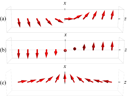
Figure 1: Schematic pictures of DW configurations employed in this paper. Red arrows denote the directions of localized magnetic moments. DWs are set up around the $xy$-plane $(z=0)$. (a)(b)(c) correspond to the coplanar (Neél), spiral (Bloch), and head-to-head DWs, respectively.

II.2 Band structure under domain wall

Now we are interested in the case where the local magnetization $\bm{M}_{i}$ forms a certain texture. Here we introduce three types of DW strctures, and calculate the eigenvalues and eigenstates by numerically diagonalizing the lattice Hamiltonian. Taking the DW parallel to the $xy$-plane, $x$- and $y$-directions can be diagonalized analytically by the Fourier transformation, while $z$-direction is no longer translationally invariant and hence it is treated numerically. Thus, we treat the system as a series of slabs stacked in $z$-direction. We introduce three types of configurations of the DW. There are two ways to twist the magnetization from $\bm{M}=-M_{0}\bm{e}_{x}$ on the one end to $\bm{M}=M_{0}\bm{e}_{x}$ on the other, as shown in Fig. 1 (a) and (b). In case (a), the magnetization points perpendicular to the DW at the center of the DW, which is called “Neél DW” or “coplanar DW”. In case (b), the magnetization is always in the DW plane, which is called “Bloch DW” or “spiral DW”. On the other hand, twisting pattern of the magnetization from $\bm{M}=M_{0}\bm{e}_{z}$ to $\bm{M}=-M_{0}\bm{e}_{z}$ can be uniquely constructed due to cubic symmetry, as shown in Fig. 1 (c), which we refer to as the “head-to-head DW”.

We first focus on the band structure under these DWs. We here set the periodic boundary condition for all directions, to exclude the effect from the surface. The size of the system in $z$-direction is given by $L_{z}=N_{z}a$, where the number of slabs $N_{z}$ is fixed to 32 here. The $x$- and $y$- directions are Fourier transformed due to the translational invariance, with the wave vector $(k_{x},k_{y})$. Therefore, the eigenstates and the eigenvalues can be labeled as $\psi_{k_{x},k_{y},n}(z)$ and $\epsilon_{k_{x},k_{y},n}$, where $n$ is the label for energy level. The wave function $\psi_{k_{x},k_{y},n}(z)$ consists of four components in the spin and pseudospin (chirality) spaces.

The coplanar and spiral DWs under the periodic boundary condition are defined by

$$\bm{M}_{\rm c}(z) =M_{0}\left(\cos{2\pi\frac{z}{L_{z}}},\ 0,\ \sin{2\pi\frac{z}{L_{z}}}\right)$$ (15)

$$\bm{M}_{\rm s}(z) =M_{0}\left(\cos{2\pi\frac{z}{L_{z}}},\ \sin{2\pi\frac{z}{L_{z}}},\ 0\right),$$ (16)

respectively, which consist of a pair of opposite DWs per each period, namely a magnetic spiral. Since the coplanar and the head-to-head configurations are equivalent by a translation by $L_{z}/4$ in the $z$-direction in this case, we do not take into account the band structure under the head-to-head configuration explicitly. We also take the uniform magnetization as a reference, where all the localized magnetic moments are pointing in $x$-direction $(\bm{M}=M_{0}\bm{e}_{x})$.

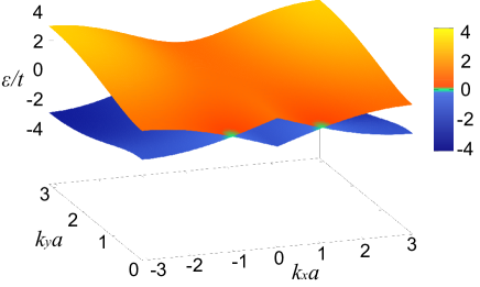
Figure 2: Band structure under the uniform magnetization $\bm{M}=M_{0}\bm{e}_{x}$, picking up the two bands crossing at zero energy. The region in the vicinity of zero energy is shown in green. Only half of the Brillouin zone $(k_{y}>0)$ is shown to clarify the crossing points of the Weyl cones.

By numerically diagonalizing the lattice Hamiltonian, we straightforwardly obtain the band structure as a function of the in-plane wave vector $(k_{x},k_{y})$ for each DW configuration. We here extract two bands crossing at zero energy, which may show the most typical behavior among all bands. Due to particle-hole symmetry, there emerge electron (orange) and hole (blue) bands touching at zero energy, as shown in Figs. 2 and 3. Under the uniform magnetization $\bm{M}=M_{0}\bm{e}_{x}$, time-reversal symmetry is broken and the two Weyl points are split in $k_{x}$-direction, as estimated in Eq. (14) (see Fig. 2).

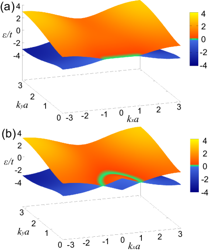
Figure 3: Band structures under the coplanar and spiral magnetization textures, with two bands picked up as in Fig. 2. (a) The electronic spectrum under the coplanar DW shows the straight “Fermi arc” between two Weyl points. (b) The Fermi arc for the spiral DW shows the circular structure, following the trajectory of the Weyl points.

On the other hand, in the presence of a DW, the electron and hole bands touch by a line at zero energy, namely the “Fermi arc”, instead of the isolated Weyl points. As can be seen in Fig. 3, the coplanar DW gives a linear Fermi arc, while the spiral DW yields a circular arc (closed loop). The “Fermi arc” observed here can be regarded as the trajectory of the Weyl points; Equation (2) states that, under a (locally) uniform magnetization $\bm{M}$, the location of the Weyl point for each valley $\eta$ is determined straightforwardly by $\bm{M}$, as $\bm{K}_{\eta}=\eta\bm{A}_{5}=\eta J\bm{M}/v_{\rm F}$. As long as the spatial variation of $\bm{M}(z)$ is sufficiently slow, the positions of the Weyl points in the $(k_{x},k_{y})$-plane can well be regarded as a function of $z$. By following the magnetization from $z=0$ to $L_{z}$, the Weyl points draw either linear or circular trajectories, depending on the type of the DW.

Since the Fermi arc found here emerges inside the DW, it cannot be measured directly, e.g. by ARPES. However, it alters the electron energy and the charge distribution of the system, which we shall discuss in the following sections.

III Excitation energy of domain wall

In this section, we estimate the excitation energy of a DW, to find out which DW configuration is the most stable. We first calculate the excitation energy numerically by comparing the total electron energy with that under a uniform magnetization. We also compare our results with the free energy that was analytically derived in the continuum limit in the previous work Araki_corr .

III.1 Numerical calculation

Here we investigate the effect of a single DW fixed around $z=0$, with $z\in[-L_{z}/2,L_{z}/2]$. The sizes of the system in $x$- and $y$-direction are given by $L_{x}=N_{x}a$ and $L_{y}=N_{y}a$, and we take here $N_{x}=N_{y}\simeq 1000$; note that $N_{x}$ and $N_{y}$ only determine the mesh in $(k_{x},k_{y})$-plane and have no physical importance. We employ the open boundary condition at $z=\pm L_{z}/2$ (i.e. exposed to vacuum), while $x$- and $y$-directions are set periodic. The DW configuration for each type is defined by

$$\bm{M}_{\rm c}(z) =M_{0}\left(\tanh\frac{z}{W},\ 0,\ \operatorname{sech}\frac{z}{W}\right)$$ (17)

$$\bm{M}_{\rm s}(z) =M_{0}\left(\tanh\frac{z}{W},\ \operatorname{sech}\frac{z}{W},\ 0\right)$$ (18)

$$\bm{M}_{\rm h}(z) =M_{0}\left(\operatorname{sech}\frac{z}{W},\ 0,\ -\tanh\frac{z}{W}\right),$$ (19)

with $W$ the width of the DW. The subscripts c, s, and h represent the coplanar, spiral, and head-to-head DWs, respectively, which we shall use in the results below.

The excitation energy of a DW is given by evaluating the energy of the electrons in the occupied states. Taking the electron chemical potential $\mu$ fixed to charge neutrality, the energy per unit area to excite a DW from the uniform magnetization is defined by

$$E_{\rm DW}=\frac{1}{L_{x}L_{y}}\sum_{\epsilon\leq 0}\epsilon_{k_{x},k_{y},n}^{\rm(DW)}-\frac{1}{L_{x}L_{y}}\sum_{\epsilon\leq 0}\epsilon_{k_{x},k_{y},n}^{\rm(uniform)},$$ (20)

where $\epsilon_{k_{x},k_{y},n}^{\mathrm{(DW)}}$ is the single-particle energy for each eigenstate under the DW, while $\epsilon_{k_{x},k_{y},n}^{\mathrm{(uniform)}}$ is the energy under the uniform magnetization. The reference uniform magnetization is taken $\bm{M}=M_{0}\bm{e}_{x}$ for the coplanar and spiral DWs, and $\bm{M}=M_{0}\bm{e}_{z}$ for the head-to-head DW. Figure 4 shows $E_{\mathrm{DW}}$ for each DW configuration as a function of the DW size $W$; we can see that the spiral DW requires the largest excitation energy among the three types, while the head-to-head DW the smallest. It can be qualitatively understood in terms of the number of zero modes. We have seen that there evolves a new “Fermi arc” state connecting the two Weyl points by introducing a DW to the magnetic texture, which means that a DW excites a bulk electron on the Weyl cone in the Fermi sea onto the Fermi arc at zero energy. Since the Fermi arc under the spiral DW is longer than that under the coplanar DW, we can estimate that the number of zero modes under the spiral DW is larger than that under the coplanar DW. Thus the DW Fermi arc accounts for the difference of the excitation energy depending on the DW configuration.

III.2 Domain wall energy in continuum limit

If the DW size $W$ is large enough, we can estimate the DW energy analytically in terms of the gradient expansion as well. Starting from the continuum Hamiltonian [Eq. (1)] and integrating out the fermionic degrees of freedom, the free energy functional $F[\bm{M}]$ for the magnetic texture $\bm{M}(\bm{r})$ was obtained in Ref. Araki_corr, as

$$F[\bm{M}] =F_{0}[\bm{M}]+F_{1}[\bm{M}]$$ (21)

$$F_{1}[\bm{M}] =\int d^{3}\bm{r}\left(J_{\rm i}\left[\bm{\nabla}\bm{M}\right]^{2}+J_{\rm a}\left[\bm{\nabla}\times\bm{M}\right]^{2}\right),$$ (22)

with shorthand notations $\left[\bm{\nabla}\bm{M}\right]^{2}=\sum_{i,j}\left(\partial_{i}M_{j}\right)^{2}$ and $\left[\bm{\nabla}\times\bm{M}\right]^{2}=\sum_{i}\left(\bm{\nabla}\times\bm{M}\right)_{i}^{2}$. The coefficients $J_{\mathrm{i}}$ and $J_{\mathrm{a}}$ are given as

$$J_{\mathrm{i}}=\frac{J^{2}}{48\pi^{2}v_{\mathrm{F}}^{3}}\frac{1}{10},\quad J_{\mathrm{a}}=\frac{J^{2}}{48\pi^{2}v_{\mathrm{F}}^{3}}\left[\ln\frac{k_{\mathrm{C}}}{k_{\mathrm{F}}}-\frac{11}{15}\right],$$ (23)

where $k_{\mathrm{F}}=\mu/v_{\mathrm{F}}$ is the Fermi momentum and $k_{\mathrm{C}}$ is the momentum cutoff that characterizes the size of the Brillouin zone.

$F_{0}[\bm{M}]$ is the homogeneous part of the free energy, which is determined only by the magnitude of the local magnetization (i.e. $|\bm{M}(\bm{r})|^{2}$) and makes no difference among the DW configurations employed here. On the other hand, the inhomogeneous part $F_{1}[\bm{M}]$ depends on the spatial texture, and is minimized under the uniform magnetization. This part consists of two terms: the first term with the coefficient $J_{\mathrm{i}}$ comes from the Fermi surface. This term has the same form as the conventional Heisenberg-like RKKY interaction, namely the effective interaction between localized spins mediated by the spin of conduction electrons. The second term with $J_{\mathrm{a}}$ originates from the interband transition process between the electron and hole bands induced by the scattering by a localized magnetic moment, which is known as the Van Vleck mechanism. Spin mixing by spin-orbit coupling is essential in the Van Vleck mechanism, hence strong spin-momentum locking around the Weyl points in this system largely enhances this term, which is captured as the logarithmic divergence in $J_{\mathrm{a}}$ for $k_{\mathrm{F}}\rightarrow 0$. Therefore, in the vicinity of the Weyl points (i.e. $\mu\sim 0$), $J_{\mathrm{a}}$-term is dominant and $J_{\mathrm{i}}$-term can be safely neglected.

Using Eq. (22) and neglecting $J_{\mathrm{i}}$-term, the free energy per unit area $f_{1}=F_{1}/A$ for each DW configuration is given by

$$f_{1}[\bm{M}_{\mathrm{c}}]=\frac{4J_{\rm a}}{3W},\ f_{1}[\bm{M}_{\mathrm{s}}]=\frac{2J_{\rm a}}{W},\ f_{1}[\bm{M}_{\mathrm{h}}]=\frac{2J_{\rm a}}{3W},$$ (24)

with $A$ the area of the DW. We can see that the spiral DW requires the largest excitation energy and the head-to-head the smallest in continuum limit, which is a complementary result with our numerical results on the lattice. The quantitative discrepancy comes from the sharp spatial variation in the magnetic texture around the center of the DW, which makes the gradient expansion less reliable.

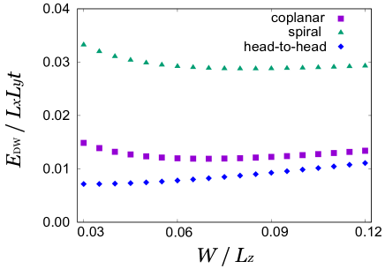
Figure 4: The excitation energy of DW at $\mu=0$ as a function of the DW width $W$, which is obtained from Eq. (20). The excitation energy of the spiral DW is the largest among all the three DW textures.

IV Localized charge

In this section, we focus on the electric charge distribution altered by the DW, using the eigenstate wavefunctions obtained by the numerical diagonalization. In a WSM with a uniform magnetization, all the eigenstates are composed of plane waves and consequently the charge distribution is uniform in the bulk. On the other hand, a magnetic DW in a WSM hosts a linearly dispersed Fermi arc mode, which may contribute to the localized charge. Here we numerically calculate the deviation of the charge distribution under the DWs from that in the uniform system. We show that a certain amount of charge gets localized around the DW, and calculate the amount of the localized charge for each DW configuration. We shall employ the same DW configuration as in the previous section for our numerical calculation.

IV.1 Charge distribution

Taking the summation over the wave function distributions over all the occupied eigenstates, we can estimate the charge distribution induced by the DW as

$$\delta\rho(z)=\frac{e}{L_{x}L_{y}a}\sum_{k_{x},k_{y}}\sum_{\epsilon\leq\mu}\left[|\psi_{k_{x},k_{y},n}^{\rm(DW)}(z)|^{2}-|\psi_{k_{x},k_{y},n}^{\rm(uniform)}(z)|^{2}\right],$$ (25)

with $e$ an elementary charge, for each DW configuration. Here $\psi_{k_{x},k_{y},n}^{\mathrm{(DW)}}(z)$ and $\psi_{k_{x},k_{y},n}^{\mathrm{(uniform)}}(z)$ denote the eigenfunction under the DW texture and that under the uniform magnetization, respectively. Figure 5 shows our calculation result, for the chemical potential $\mu=0.1t$ and the DW size $W=0.1L_{z}$. We can see here that charge is accumulated around the DW for all the three DW configurations. We should note that the coplanar and the spiral DWs give a single peak at the center of the DW, while the head-to-head type gives two peaks separated by a small cusp at the center.

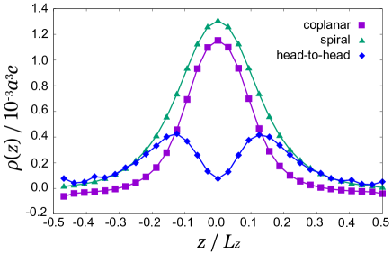
Figure 5: The charge distribution calculated by Eq. (25), with $\mu/t=0.1$ and $W/L_{z}=0.1$. The coplanar and the spiral DWs give a single large peak, while the head-to-head DW gives two small peaks.

The charge localization found here can be traced back to the Landau quantization under the axial magnetic field. As we have seen in Eq. (2), the local magnetization $\bm{M}(\bm{r})$ couples to the electron spin as an axial gauge field $\bm{A}_{5}(\bm{r})=(J/ev_{F})\bm{M}(\bm{r})$ at low energy. The magnetic DW texture bears a vorticity inside the DW, which corresponds to the axial magnetic field,

$$\bm{B}_{5}(\bm{r})=\bm{\nabla}\times\bm{A}_{5}(\bm{r}).$$ (26)

Using the formulations in Eqs. (17)-(19), the axial magnetic field distribution for each DW configuration is given by

$$\bm{B}_{5\mathrm{c}}(z) =\frac{JM_{0}}{ev_{\rm F}}\left(0,\ \operatorname{sech}^{2}\frac{z}{W},\ 0\right)$$ (27)

$$\bm{B}_{5\mathrm{s}}(z) =\frac{JM_{0}}{ev_{\rm F}}\left(\tanh\frac{z}{W}\operatorname{sech}\frac{z}{W},\ \operatorname{sech}^{2}\frac{z}{W},\ 0\right)$$ (28)

$$\bm{B}_{5\mathrm{h}}(z) =\frac{JM_{0}}{ev_{\rm F}}\left(0,\ -\tanh\frac{z}{W}\operatorname{sech}\frac{z}{W},\ 0\right).$$ (29)

It should be noted that the direction of the axial magnetic field, i.e. $\hat{\bm{B}}_{5}(z)\equiv\bm{B}_{5}(z)/|\bm{B}_{5}(z)|$, is unidirectional ($y$-direction) for the coplanar DW, while it spatially varies for the spiral and head-to-head cases. $\bm{B}_{5\mathrm{h}}(z)$ suddenly flips its direction at the DW center, while $\bm{B}_{5\mathrm{s}}(z)$ gradually changes its direction inside the DW.

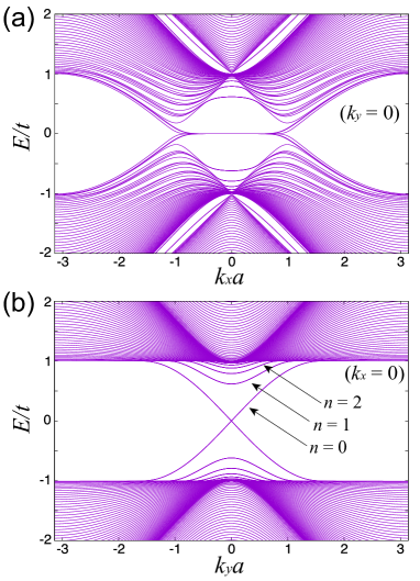
Figure 6: The band structure in the presence of two opposite coplanar DWs under the periodic boundary condition, with (a) $k_{y}=0$ and (b) $k_{x}=0$. The bands show the Landau-like spectrum around zero energy, with the zeroth LL $(n=0)$ unidirectionally dispersed in $k_{y}$-direction.

The axial magnetic field induces the Landau quantization in the electronic spectrum, just like a normal (realistic) magnetic field Liu_2013 . In the presence of a uniform axial magnetic field $\bm{B}_{5}=B_{5}\bm{e}_{y}$, for instance, the Landau level (LL) spectrum for the $n$-th LL $(n=0,\pm 1,\pm 2,\cdots)$ is given by

$$E_{n\neq 0}(k_{y}) =v_{\mathrm{F}}\mathrm{sgn}(n)\sqrt{2|n|eB_{5}+k_{y}^{2}}$$ (30)

$$E_{n=0}(k_{y}) =v_{\mathrm{F}}k_{y},$$ (31)

where the zeroth LL is unidirectionally dispersed along the axial magnetic field Liu_2013 ; K-Y_Yang . Figure 6 shows the band structure in the presence of coplanar DWs calculated by the numerical diagonalization DW-note ; it shows the Landau-like spectrum around zero energy, which comes from the axial magnetic field arising from the DW texture.

Here we should note that the Landau states localize at the magnetic flux, with the degeneracy $\rho=B_{5}/\phi_{0}$ per unit area, where $\phi_{0}=e/2\pi$ is the flux quantum. This implies that, in the presence of a spatial variation in $\bm{B}_{5}$, the charge density becomes larger in the region where the amplitude of $\bm{B}_{5}$ is strong. Figure 7 shows the spatial distribution of $|\bm{B}_{5}(z)|$ for each DW texture, all of which show strong $|\bm{B}_{5}|$ around the center of the DW. Comparing the charge distribution in Fig. 5 and the axial magnetic field distribution in Fig. 7, we can regard the charge localization as the result of the Landau quantization and degeneracy by the axial magnetic field at the DW. For instance, the spiral DW gives the strongest axial magnetic field among the three DW configurations, which leads to the largest localized charge, as seen in the calculation. The two-peak structure in the charge distribution in the presence of the head-to-head DW can also be traced back to the strength of the corresponding axial magnetic field. Since the wave function of each Landau state has a tail at a scale of the cyclotron radius, the charge density at $z=0$ becomes finite even though the axial magnetic field reaches zero there.

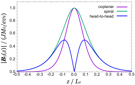
Figure 7: The strength of the axial magnetic field $\bm{B}_{5}$ for each DW configuration. $|\bm{B}_{5}|$ for the head-to-head DW has two peaks and vanishes at $z=0$, which accounts for the cusp structure in the charge distribution seen in Fig. 5.

If the Fermi level is fixed to zero energy, the contribution from the occupied LLs is negligible; while the charge density coming from the bulk states is proportional to the volume of the Brillouin zone, namely $k_{\mathrm{C}}^{3}$, that from the Landau states is proportional to the length of the Brillouin zone, namely $\rho k_{\mathrm{C}}$. Therefore, at charge neutrality, the charge distribution becomes completely flat in the continuum limit (i.e. $k_{\mathrm{C}}\rightarrow\infty$), except for the surface of the sample. On the other hand, when the Fermi level is set slightly above or below zero energy, the deviation of the charge distribution from charge neutrality mainly comes from the zeroth LL; the density of states in the zeroth LL is constant around $\mu=0$, while that for Weyl cones is quadratic in $\mu$. The relation between the localized charge and the chemical potential shall be discussed further in the next subsection.

IV.2 Total localized charge

The net charge $q$ localized at the DW is obtained by integrating the charge distribution over the whole system,

$$q =\sum_{z}\delta\rho(z)a$$ (32)

$$=\frac{e}{N}\sum_{k_{x},k_{y},z}\sum_{\epsilon\leq\mu}\left[|\psi_{k_{x},k_{y},n}^{\rm(DW)}(z)|^{2}-|\psi_{k_{x},k_{y},n}^{\rm(uniform)}(z)|^{2}\right],$$

per unit area of the DW. Figure 8 shows the behavior of the total charge as a function of the chemical potential $\mu$ for each DW configuration, with the DW width $W$ fixed to $0.1L_{z}$. We can see that the spiral DW bears the largest charge and the head-to-head DW the smallest, as we have seen in the charge distribution calculation. It should be noted that the total charge is almost proportional to the chemical potential $\mu$ for any DW configuration, since the number of the occupied states in the lowest LL is proportional to $\mu$ due to its constant density of states around $\mu=0$. When the chemical potential $\mu$ goes beyond the energy scale $\sim 0.1t$, which is not shown in Fig. 8, the total charge $q$ becomes no longer proportional to $\mu$, since not only the zeroth LL but the higher LLs also gets occupied and contribute to the localized charge.

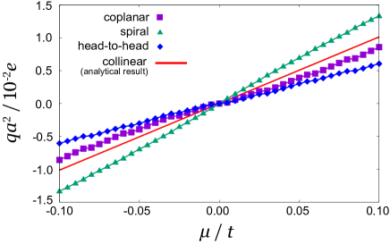
Figure 8: The net localized charge $q$ as a function of the chemical potential $\mu$ for each DW, with the DW size $W=0.1L_{z}$. The net localized charge at the collinear DW, which was analytically obtained in Ref. Araki_DW, [Eq. (34)], is shown by the red solid line for comparison.

Under a certain DW configuration, the Weyl equation under the continuum Hamiltonian [Eq. (1)] can be analytically solved to estimate the amount of the localized charge. In Ref. Araki_DW, , the authors employed the simplified collinear DW configuration, which is described by the magnetic texture

$$\bm{M}_{\mathrm{coll}}(z)=M_{0}\left(\tanh\frac{z}{W},\ 0,\ 0\right),$$ (33)

and derived the net localized charge

$$q_{\mathrm{coll}} =\frac{e}{\pi^{2}}\frac{k_{\Delta}}{v_{\rm F}}\mu$$ (34)

by using the distribution of the analytically obtained wavefunctions in the zeroth LL. Since the axial magnetic field structure of the collinear DW is identical to that of the coplanar DW, this analytical form applies to the coplanar DW as well. In Fig. 8, we also show this analytical form in the solid red line. It is in good agreement with the numerically obtained $q$ for the coplanar DW, from which we can ensure that the charge localization around the DW is dominated by the zeroth LL, as assumed in Ref. Araki_DW, .

The localized charge confirmed here implies that, when the DW is moving adiabatically (e.g. by an external magnetic field), it carries the localized charge, resulting in a current pulse. Based on this charge pumping picture, the localized charge was conversely estimated in Ref. Araki_pumping, , as

$$q=\frac{e}{2\pi^{2}}\frac{J\mu}{v_{\mathrm{F}}^{2}}\int dz|\partial_{z}\bm{M}_{\perp}(z)|=\frac{e^{2}}{2\pi^{2}}\frac{\mu}{v_{\mathrm{F}}}\int dz|\bm{B}_{5\perp}(z)|,$$ (35)

where the subscript $\perp$ denotes vector components transverse to the $z$-axis. This relation was derived by assuming the quantum limit of the Landau quantization, requiring the Fermi level $\mu$ to be low enough so that it should be between the zeroth and first LLs under the axial magnetic field $\bm{B}_{5}(z)$ throughout the whole system. Under this assumption, Eq. (35) gives the localized charge per unit area of the coplanar(c), spiral(s), and head-to-head(h) DWs as

$$q_{\mathrm{c}}=q_{\mathrm{h}}=\frac{e}{\pi^{2}}\frac{JM_{0}}{v_{\mathrm{F}}^{2}}\mu,\quad q_{\mathrm{s}}=\frac{e}{2\pi}\frac{JM_{0}}{v_{\mathrm{F}}}\mu.$$ (36)

For the coplanar DW, this relation is consistent with that from the analytical diagonalization given in Eq. (34), namely the solid red line in Fig. 8. Comparing these relations with our numerical results in the present work, we find that Eq. (36) overestimates the localized charge for the head-to-head DW. Such a discrepancy can presumably be traced back to the breakdown of the quantum limit assumption; since the axial magnetic field drops sharply to zero at the center of the head-to-head DW, the quantum limit assumption is no longer reliable about the center of the DW. On the other hand, Eq. (36) well describes our numerical results for the coplanar and spiral DWs, since the axial magnetic field for these DWs is strong enough to apply the quantum limit assumption within the region of the DW. Since the size of the system is finite in our numerical calculation, we lose the “tail” of the localized charge beyond the boundary, which slightly reduces the net charge $q$ from its analytically obtained value in the infinite system.

IV.3 Physical implications

Let us now discuss how the localized charge at the DW can be captured experimentally. Regarding the system as Cr-doped $\mathrm{Bi_{2}Se_{3}}$ (Ref. Kurebayashi_2014, ), we can estimate the amount of the localized charge with Eq. (34) for the coplanar DW. We take the Fermi velocity (within the quintuple layer) as $v_{\mathrm{F}}=3.55\mathrm{eV}\text{\AA}$, which was observed by the ARPES measurement Kuroda_2010 . From the first-principles calculation Yu_R , the exchange coupling between the localized magnetic moment of Cr and the p-electron was estimated as $JM_{0}=2.7\mathrm{eV}$. In the present system, since Cr is doped by partially substituting Bi to the concentration $x$, we use $xJM_{0}$ instead of $JM_{0}$ in our calculation, by taking the local average of the exchange energy around each site; here we use $x=0.05$, which was suggested by Ref. Kurebayashi_2014, . By using the parameters given above, and tuning the chemical potential $\mu$ to $100\mathrm{meV}$, the localized charge on the coplanar DW is obtained as

$$q=1.1e\times 10^{11}\mathrm{cm}^{-2}.$$ (37)

Therefore, for a DW with its size $W=10\mathrm{nm}$, the average charge density inside the DW is given as $q/W=1.1e\times 10^{18}\mathrm{cm}^{-3}$. This value is comparable to the typical charge density in GaAs, which implies that the localized charge may be directly measured by the scanning tunneling microscope (STM) in a thin-film geometry Wiesendanger .

Moreover, since the DW behaves as a charged object, we can expect that an external electric field applied to this system can drive the motion of the DW. Here we should note that the electron transmission beyond the DW is suppressed if the chirality-flipping scattering process is negligible, since the DW drastically exchange the positions of the valleys in the Brillouin zone Kobayashi_2018 . Therefore, the DW in our magnetic WSM is driven only by the electrostatic force, which is distinct from the well-known spin-transfer and spin-orbit torques invoked by the conduction electron. Such a driving force may be more advantageous than that by the current-induced torques, in that it can reduce the energy loss by Joule heating.

The creep velocity of the DW can be roughly estimated by the semiclassical equation of motion for a DW. In the absence of a pinning potential, the dynamics of the DW obeys a simple Newtonian equation of motion Doring

$$M_{W}\ddot{X}+\frac{M_{W}}{\tau_{W}}\dot{X}=qE$$ (38)

for a DW per unit area under the electric field $E$, where $X$ denotes the center of mass of the DW in the collective coordinate representation. The “inertial mass” (per unit area) $M_{W}=N_{W}/KW^{2}$ comes from the moment of inertia of each localized spin against the external torque, while the “friction factor” $\tau_{W}^{-1}=\alpha K/\hbar$ arises from the Gilbert damping; here $N_{W}=2xW/a^{3}$ is the number of localized spins in a unit area of the DW, $a$ is the lattice constant, $K$ is the magnetic anisotropy energy, and $\alpha$ is the Gilbert damping constant. If the Gilbert damping is sufficiently large, the driving force here leads to an adiabatic motion of the DW. The DW velocity $V$ eventually reaches a constant value, namely the creep velocity,

$$V_{\mathrm{C}}=\frac{\tau_{W}}{M_{W}}qE=\frac{a^{3}W}{2\alpha x}qE.$$ (39)

We should note that this creep velocity becomes independent of the Cr concentration $x$ as long as the localized charge $q$ comes only from the zeroth LL, since $q$ is proportional to the (averaged) exchange energy $xJM_{0}$ in this regime, as we have seen in the discussion above. Using the lattice constant $a=9.84\mathrm{\AA}$ employed for the first-principles calculation on $\mathrm{Bi_{2}Se_{3}}$ (Ref. Mishra, ) and fixing the Gilbert damping constant to the typical value $\alpha=0.01$, the localized charge $q$ obtained in Eq. (37) for the coplanar DW yields the creep velocity $V_{\mathrm{C}}=81\mathrm{m/s}$ under the electric field $E=100\mathrm{V/cm}$. This velocity is not as fast as the typical DW velocity driven by spin-orbit torques, which can reach up to 300-400 m/s (see Refs. Emori, and Ryu_K-S, ). However, our method using WSMs is still advantageous in the energetic efficiency, i.e. the reduction of the Joule heating.

V Conclusion

In this paper, we have investigated the electronic properties of a magnetic WSM in the presence of magnetic DWs. Using the energy eigenvalues and eigenstates obtained from the numerical diagonalization of the magnetic Weyl Hamiltonian, we have calculated the DW excitation energy and the charge distribution for three types of DWs: coplanar, spiral, and head-to-head. The main finding in this paper is that a DW in a magnetic WSM induces a localized charge at the DW, the amount of which linearly depends on the Fermi level for any type of DW at low energy. We can understand this behavior by regarding the magnetic texture as an emergent axial magnetic field for the electrons: as the magnetic DW texture is equivalent to the axial magnetic field around the center of the DW, it yields Landau quantized states at the DW, and the zeroth LL among them contributes to the localized charge at low energy. Since the zeroth LL in 3D is unidirectionally dispersed and shows constant density of states at low energy, the localized charge, namely the number of the occupied states, becomes proportional to the Fermi energy. The charge distribution around the DW qualitatively agrees with the spatial profile of the axial magnetic field for each DW configuration, which also supports our “Landau quantization” hypothesis.

While we have neglected the Coulomb interaction in our analysis, it usually has a significant effect on the charge distribution: when an electric charge is put inside a conductor, a charge with the opposite sign gets accumulated around the original charge due to the Coulomb interaction, which is known as the electrostatic screening. Although the localized charge in a WSM should also be subject to the screening in the presence of the Coulomb interaction, we expect that it would be less significant than that in normal metals. The screening effect in general can be neglected if the system size is smaller than the screening length: this is more likely to occur in WSMs than in normal metals, since the screening length in WSMs at low energy tends to be longer than that in normal metals due to the vanishing density of states at the Weyl points.

Making use of this localized charge, we have semiclassically demonstrated that a DW in a magnetic WSM can be driven by the electrostatic force from an external electric field. This effect can be regarded as the inverse effect of the charge pumping conveyed by the dynamics of a magnetic texture in a WSM, which was proposed in the recent paper by the authors Araki_pumping . It should be noted that the DW in this system almost totally suppresses the conduction current Kobayashi_2018 and thus will not suffer from energy loss by Joule heating, which is quite advantageous in making use of such DWs for spintronics. Recent transport and ARPES measurements found that a Heusler alloy $\mathrm{Co_{3}Sn_{2}S_{2}}$ shows the ferromagnetic WSM phase Liu_E ; Muechler ; Xu_Q , which may serve as a good playground for magnetic DWs treated in our work. On the other hand, our hypothetical lattice model cannot be straightforwardly applied to antiferromagnetic WSMs, such as $\mathrm{Mn_{3}Sn}$ (Refs. Yang_2017, ; Ito, ; Kuroda, ), since noncollinear antiferromagnetic orders on the kagome lattice are expected in those materials. In antiferromagnetic $\mathrm{Mn_{3}Sn}$, for instance, the tight-binding model calculation Ito showed that its chiral antiferromagnetic order is related to the separation of the Weyl points and the anomalous Hall conductivity. Therefore, we can make a rough qualitative assumption that a spatial modulation of the antiferromagnetic order becomes equivalent to the axial magnetic field, which implies that an antiferromagnetic DW may host the localized charge in a similar manner to the ferromagnetic DWs observed here.