Optimal community structure for social contagions

Abstract

Community structure is an important factor in the behavior of real-world networks because it strongly affects the stability and thus the phase transition order of the spreading dynamics. We here propose a reversible social contagion model of community networks that includes the factor of social reinforcement. In our model an individual adopts a social contagion when the number of received units of information exceeds its adoption threshold. We use mean-field approximation to describe our proposed model, and the results agree with numerical simulations. The numerical simulations and theoretical analyses both indicate that there is a first-order phase transition in the spreading dynamics, and that a hysteresis loop emerges in the system when there is a variety of initially-adopted seeds. We find an optimal community structure that maximizes spreading dynamics. We also find a rich phase diagram with a triple point that separates the no-diffusion phase from the two diffusion phases.

1 Introduction

Social contagion—including the spreading of social information, opinions, cultural practices, and behavior patterns—is ubiquitous in nature and society [1, 2, 3, 4]. Unlike biological contagion [5, 6], social reinforcement, which is also ubiquitous, plays a central role in social contagions and triggers such complex dynamic phenomena [7, 8, 9] as first-order phase transitions [10]. Empirical studies indicate that susceptible individuals adopt a social behavior only when the number of received information units exceeds an adoption threshold [11, 12, 13, 14]. Thus this behavior occurs when a certain level of exposure is exceeded. The numerous Markovian and non-Markovian models of complex networks used to describe social contagion [15, 16, 17, 18] indicate that the topology of networks strongly affects patterns of social contagion [19, 20, 21, 22, 23, 24, 25, 26, 27]. Recently scholars extended the social contagion model to multiplex networks and found that multiplexity promotes social contagion [28, 29, 30]. Holme et al. [31, 32] found that a temporal network in which the network structure changes with time can either promote or suppress social contagions under various scenarios. Macroscopically, researchers have found that the average degree and the level of heterogeneity of the degree distribution changes the growth patterns of social contagions [33, 34]. Microscopically, social contagions exist in a hierarchy [33], i.e., high-degree nodes or hubs are infected in the early stages of the infection process and low-degree nodes in the later stages. Mesoscopically, researchers have studied how degree correlation and community structure affect social contagion [35, 36]. Researchers have found a level of network modularity—the measurement of how strongly a network is divided into modules or communities—that is optimal. The initial number of adopter seeds that allows a global diffusion of the contagion is at its minimum [37]. Majdandzic proposed a contagion model with an adoption threshold and spontaneous adoption, and found the system has hysteresis loop and phase-flipping [38].

Most previous studies have focused on an irreversible social contagion in which infected agents either recover or die and in both cases no longer can be infected [39, 40]. These studies do not take into account the effect of reversible social contagion in which infected agents can once again be infected after passing through a susceptible period [41]. In real-world epidemics [42] individuals often are not fully immunized and return to a susceptible state after having been infected. We here present a reversible social contagion model of a community network [43, 44]. Initially a number of infected individuals are randomly distributed in the community. All other individuals are susceptible. Susceptible individuals become infected when the number of received information units exceeds their adoption thresholds. We derive our model using mean-field theory. Both numerical simulations and theoretical analyses indicate the presence of a hysteresis loop in social contagions. More important, we find an optimal network modularity that globally promotes social contagions. The constant threshold point, the critical threshold fraction of intracommunity links, triggers a sharp transition from a no-diffusion state to a global diffusion state.

This paper is organized as follows. In Sec. 2, we propose a social contagion model for community networks. In Sec. 3 we develop a mean-field theory to mathematically analyze our model. In Sec. 4 we simulate the proposed model on a community network and show the results. In Sec. 5 we discuss our conclusions.

2 Model descriptions

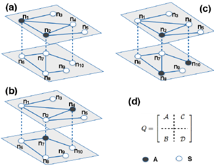
In our model the network has two equal-sized communities, $a$ and $b$, with $N$ nodes and $L$ links in the network system. Initially nodes are with equal probability assigned to either community $a$ or community $b$. Then $(1-\mu)L$ links are randomly distributed among node pairs within a community and $\mu L$ are randomly distributed among node pairs between communities $a$ and $b$. The $\mu$ value is the probability that a randomly selected link is an interlink between different communities. We adjust the strength of the social community by changing the value of $\mu$. Figure 1(d) shows a matrix of the community. Matrix $\mathcal{A}$ ($\mathcal{D}$) shows the connections among individuals within community $a$ ($b$). Matrix $\mathcal{C}$ ($\mathcal{B}$) shows the individuals in community $b$ ($a$) connected to individuals in community $a$ ($b$).

Using this topology we develop a susceptible-adopted-susceptible (SAS) social contagion model of a community network. Individuals are either susceptible (S) or adopted (A). A susceptible individual can receive information from adopted neighbors in communities $a$ and $b$. An adopted individual can transmit the social contagion to susceptible neighbors. At the initial stage, a random fraction of $\rho_{0}$ of individuals are adopted in community $a$, and the remaining individuals are susceptible in both communities. An adopted individual has adopted the behavior and with probability $\lambda$ transmits the information to susceptible neighbors that belong to both communities. If the units of information $m$ a susceptible individual has received exceeds an adoption threshold $\theta$, the susceptible individual enters the adopted state. The parameter $\theta$ indicates the willingness of an individual to adopt a new behavior. Large (small) $\theta$ values indicate that susceptible individuals need a large (small) amount of information before they enter into the adopted state. Each adopted individual with probability $\gamma$ loses interest in the social contagion and returns to the susceptible state. Figures 1(a)–1(c) schematically show this information spreading process.

Figure 1: (Color online) Schematic of two-community system where the contagion dynamics take place. The agents $n_{1}$, $n_{2}$, $n_{3}$, $n_{4}$ and $n_{5}$ are in community $a$, and $n_{6}$, $n_{7}$, $n_{8}$, $n_{9}$ and $n_{10}$ are in community $b$. (a) At time step $1$ , the agents $n_{1}$ and $n_{2}$ are in the adopted state, and the other agents are in the susceptible state. (b) At time step $2$, susceptible agents $n_{4}$ and $n_{7}$ change to the adopted state because the number of received information $m$ exceed the adoption threshold $\theta$. At the same time, the adopted agents $n_{1}$ and $n_{2}$ recover and go to the susceptible state. (c) At time step $3$, the susceptible agents $n_{2}$, $n_{8}$ and $n_{10}$ enter the adopted state because the number of received information $m$ exceed the adoption threshold $\theta$. At the same time, the adopted agents $n_{4}$ and $n_{7}$ recover and go to the susceptible state. (d) $Q$ is the adjoin matrix of the system. $\mathcal{A}$, $\mathcal{B}$, $\mathcal{C}$ and $\mathcal{D}$ are the partitioned matrix of $Q$.

3 Theory

3.1 Mathematical theory

Here we derive a mean-field theory for our model that reproduces social contagion dynamics. We denote $\rho^{\ell}_{i}(t)$ ($\ell=a$ or $b$) to be the density of individuals in community $\ell$ in the adopted state at time $t$. The dynamic equations for $\rho^{a}_{i}(t)$ and $\rho^{b}_{i}(t)$ are

$$\frac{d\rho^{a}_{i}(t)}{dt}=-\gamma\rho^{a}_{i}(t)+[1-\rho^{a}_{i}(t)]\delta(\lambda\sum_{j}\mathcal{A}_{ij}\rho_{j}^{a}(t)+\lambda\sum_{j}\mathcal{C}_{ij}\rho_{j}^{b}(t)),$$ (1)

and

$$\frac{d\rho^{b}_{i}(t)}{dt}=-\gamma\rho^{b}_{i}(t)+[1-\rho^{b}_{i}(t)]\delta(\lambda\sum_{j}\mathcal{B}_{ij}\rho_{j}^{a}(t)+\lambda\sum_{j}\mathcal{D}_{ij}\rho_{j}^{b}(t)),$$ (2)

respectively. Here $\gamma\rho^{\ell}_{i}(t)$ is the probability that an adopted individual $i$ recovers at time $t$ in community $\ell$, and $\lambda\sum_{j}\mathcal{A}_{ij}\rho_{j}^{a}$ and $\lambda\sum_{j}\mathcal{C}_{ij}\rho_{j}^{b}$ respectively are the units of information a susceptible individual $i$ in community $a$ receives from adopted neighbors in communities $a$ and $b$ at time $t$. We set $\lambda\sum_{j}\mathcal{B}_{ij}\rho_{j}^{a}$ and $\lambda\sum_{j}\mathcal{D}_{ij}\rho_{j}^{b}$ to respectively represent the units of information a susceptible individual $i$ in community $b$ receives from adopted neighbors in communities $a$ and $b$ at time $t$. The function $\delta$ is the probability that an individual becomes adopted. Thus $\delta(m)=1$ when the information received by an individual ($m$) exceeds the adoption threshold ($\theta$), i.e., when $m\geq\theta$ and zero otherwise.

Using Eqs. (1) and (2) we determine the evolution of social contagions in community networks. Note that we need $N$ differential equations to describe the spreading dynamics. When $N\rightarrow\infty$, it is difficult to solve the equations. More important, it is difficult to determine the transition points of the system. For simplicity we assume $\rho_{i}^{\ell}\equiv\rho_{i}^{\ell}(t)$, $F(\rho_{i}^{\ell})=-\gamma\rho_{i}^{\ell}(t)$, and $K(\rho_{i}^{\ell})=[1-\rho_{i}^{\ell}(t)]$. Equations (1) and (2) can be written in terms of $F(\rho_{i}^{\ell})$ and $K(\rho_{i}^{\ell})$ as

$$\frac{d\rho^{a}_{i}}{dt}=F(\rho_{i}^{a})+K(\rho_{i}^{a})\delta(\lambda\sum_{j}\mathcal{A}_{ij}\rho_{j}^{a}+\lambda\sum_{j}\mathcal{C}_{ij}\rho_{j}^{b}),$$ (3)

and

$$\frac{d\rho^{b}_{i}}{dt}=F(\rho_{i}^{b})+K(\rho_{i}^{b})\delta(\lambda\sum_{j}\mathcal{B}_{ij}\rho_{j}^{a}+\lambda\sum_{j}\mathcal{D}_{ij}\rho_{j}^{b}).$$ (4)

These equations describe the dynamic interactions of all nodes in the system. Calculating the time-dependent activities of all the interactive nodes is complex. A susceptible high-degree individual $i$ is more likely to receive information from neighbors than a susceptible small-degree individual $j$. Thus the probability that susceptible individual $i$ receives information from neighbor $j$ is proportional to the degree of $j$. Using Ref. [45] we evaluate the dynamic evolution process of a node by quantifying the average dynamics of neighbor nodes. The degree of node $j$ is $s_{j}^{Q}=\sum_{i=1}^{N}Q_{ij}$ ($Q$ is the adjacency matrix of the system). We introduce $\langle y_{j}\rangle_{nn}$ with the scalar quantity $y_{j}$ related to the degree of node $j$

$$\langle y_{j}\rangle_{nn} =\frac{\frac{1}{N}\sum_{j=1}^{N}s_{j}^{M}y_{j}}{\frac{1}{N}\sum_{j=1}^{N}s_{j}^{M}}=\frac{\bm{I^{T}My}}{\bm{I^{T}MI}}$$ (5)

$$=\frac{\langle s_{j}^{M}y_{j}\rangle}{\langle s_{j}^{M}\rangle}=\mathfrak{C}(\bm{y})_{M},$$

where $M\in\{\mathcal{A},\mathcal{B},\mathcal{C},\mathcal{D}\}$, $\bm{I}=(1,\ldots,1)^{T}$, $\bm{y}=(y_{1},\ldots,y_{N})^{T}$, and $\mathfrak{C}(\bm{y})_{M}$ is an operator, which is the nearest neighbor average to the explicit summation. From Eq. (5) we know that higher degree nodes contribute more to $\langle y_{j}\rangle_{nn}$. If we assume $y_{j}(\rho_{j}^{\ell})=\rho_{j}^{\ell}$, Eqs. (3) and (4) can be rewritten

$$\frac{d\rho^{a}_{i}}{dt}=F(\rho_{i}^{a})+K(\rho_{i}^{a})\delta(\lambda s_{i}^{\mathcal{A}}\mathfrak{C}(\bm{\rho_{a}})_{\mathcal{A}}+\lambda s_{i}^{\mathcal{C}}\mathfrak{C}(\bm{\rho_{b}})_{\mathcal{C}}),$$ (6)

and

$$\frac{d\rho^{b}_{i}}{dt}=F(\rho_{i}^{b})+K(\rho_{i}^{b})\delta(\lambda s_{i}^{\mathcal{B}}\mathfrak{C}(\bm{\rho_{a}})_{\mathcal{B}}+\lambda s_{i}^{\mathcal{D}}\mathfrak{C}(\bm{\rho_{b}})_{\mathcal{D}}),$$ (7)

where $\bm{\rho_{\ell}}=(\rho_{1}^{\ell},\rho_{2}^{\ell},\cdots,\rho_{n}^{\ell})^{\rm T}$. Inspired by Ref. [45] we use equations Eqs. (6) and (7) to describe the spreading dynamics and rewrite them in terms of vectors,

$$\frac{d\bm{\rho_{a}}}{dt}=F(\bm{\rho_{a}})+K(\bm{\rho_{a}})\delta(\lambda\bm{s_{\mathcal{A}}}\mathfrak{C}(\bm{\rho_{a}})_{\mathcal{A}}+\lambda\bm{s_{\mathcal{C}}}\mathfrak{C}(\bm{\rho_{b}})_{\mathcal{C}}),$$ (8)

and

$$\frac{d\bm{\rho_{b}}}{dt}=F(\bm{\rho_{b}})+K(\bm{\rho_{b}})\delta(\lambda\bm{s_{\mathcal{B}}}\mathfrak{C}(\bm{\rho_{a}})_{\mathcal{B}}+\lambda\bm{s_{\mathcal{D}}}\mathfrak{C}(\bm{\rho_{b}})_{\mathcal{D}}),$$ (9)

where $\bm{s_{M}}=(s_{1}^{M},s_{2}^{M},\cdots,s_{n}^{M})^{\rm T}$. From Eqs. (8) and (9) we obtain the fraction of infected nodes. When $t\rightarrow\infty$ we denote the final behavior adoption size in community $a$ and $b$ to be $\rho_{a}$ and $\rho_{b}$, respectively. The final behavior adoption size of the system is $\rho=\rho_{a}+\rho_{b}$.

3.2 Threshold points

Another important factor in the spreading dynamics concerns any existing threshold points. To obtain them we linearize Eqs. (8) and (9) around $\bm{\rho}_{\ell}=0$ ($\ell\in\{a,b\}$),

$$\frac{d\mathfrak{C}(\bm{\rho_{a}})_{\mathcal{M}}}{dt} =F(\mathfrak{C}(\bm{\rho_{a}})_{\mathcal{M}})+K(\mathfrak{C}(\bm{\rho_{a}})_{\mathcal{M}})\delta(\lambda\mathfrak{C}(\bm{s_{\mathcal{A}}})_{\mathcal{M}}\mathfrak{C}(\bm{\rho_{a}})_{\mathcal{A}}$$ (10)

$$+\lambda\mathfrak{C}(\bm{s_{\mathcal{C}}})_{\mathcal{M}}\mathfrak{C}(\bm{\rho_{b}})_{\mathcal{C}}),$$

and

$$\frac{d\mathfrak{C}(\bm{\rho_{b}})_{\mathcal{N}}}{dt} =F(\mathfrak{C}(\bm{\rho_{b}})_{\mathcal{N}})+K(\mathfrak{C}(\bm{\rho_{b}})_{\mathcal{N}})\delta(\lambda\mathfrak{C}(\bm{s_{\mathcal{B}}})_{\mathcal{N}}\mathfrak{C}(\bm{\rho_{a}})_{\mathcal{B}}$$ (11)

$$+\lambda\mathfrak{C}(\bm{s_{\mathcal{D}}})_{\mathcal{N}}\mathfrak{C}(\bm{\rho_{b}})_{\mathcal{D}}),$$

where $\mathcal{M}\in\{\mathcal{A},\mathcal{B}\}$, and $\mathcal{N}\in\{\mathcal{C},\mathcal{D}\}$. To obtain the threshold points, we solve the above system with $N$ equations, but it is difficult to obtain the analytic value. Thus we reduce the dimensionality of the system by introducing an operator [45].

The probability $\rho_{{\rm eff},M}^{\ell}$ that nodes in community $\ell$ are infected by neighbors in community $M\in\{\mathcal{A},\mathcal{B},\mathcal{C},\mathcal{D}\}$ is

$$\rho_{{\rm eff},M}^{\ell}=\mathfrak{C}(\bm{\rho_{\ell}})_{M}=\frac{\bm{I^{T}M\rho_{\ell}}}{\bm{I^{T}MI}}=\frac{\langle s^{M}_{j}\rho^{\ell}_{j}\rangle}{\langle s^{M}_{j}\rangle}.$$ (12)

We define $\beta_{U,M}$ ($U\in\{\mathcal{A},\mathcal{B},\mathcal{C}$, $\mathcal{D}\}$) to be

$$\beta_{U,M}=\mathfrak{C}(\bm{s_{U}})_{M}=\frac{\bm{I^{T}Ms_{U}}}{\bm{I^{T}MI}}=\frac{\langle s^{M}_{j}s^{U}_{j}\rangle}{\langle s^{M}_{j}\rangle}.$$ (13)

Inserting Eqs. (12) and (13) into Eqs. (10) and (11), we obtain

$$\frac{{d\rho_{{\rm eff},\mathcal{M}}^{a}}}{dt}=F(\rho_{{\rm eff},\mathcal{M}}^{a})+K(\rho^{a}_{{\rm eff},\mathcal{M}})\delta(\lambda\beta_{\mathcal{A},\mathcal{M}}\rho_{{\rm eff},\mathcal{A}}^{a}+\lambda\beta_{\mathcal{C},\mathcal{M}}\rho_{{\rm eff},\mathcal{C}}^{b}),$$ (14)

and

$$\frac{{d\rho_{{\rm eff},\mathcal{N}}^{b}}}{dt}=F(\rho_{{\rm eff},\mathcal{N}}^{b})+K(\rho^{b}_{{\rm eff},\mathcal{N}})\delta(\lambda\beta_{\mathcal{B},\mathcal{N}}\rho_{{\rm eff},\mathcal{B}}^{a}+\lambda\beta_{\mathcal{D},\mathcal{N}}\rho_{{\rm eff},\mathcal{D}}^{b}).\\$$ (15)

In the steady state we have $d\rho_{{\rm eff},\mathcal{M}}^{a}/dt=0$ and $d\rho_{{\rm eff},\mathcal{N}}^{b}/dt=0$. Thus we have

$$f(\rho_{{\rm eff},\mathcal{M}}^{a},\rho_{{\rm eff},\mathcal{N}}^{b})=F(\rho_{{\rm eff},\mathcal{M}}^{a})+K(\rho^{a}_{{\rm eff},\mathcal{M}})\delta(\lambda\beta_{\mathcal{A},\mathcal{M}}\rho_{{\rm eff},\mathcal{A}}^{a}+\lambda\beta_{\mathcal{C},\mathcal{M}}\rho_{{\rm eff},\mathcal{C}}^{b}),$$ (16)

and

$$g(\rho_{{\rm eff},\mathcal{M}}^{a},\rho_{{\rm eff},\mathcal{N}}^{b})=F(\rho_{{\rm eff},\mathcal{N}}^{b})+K(\rho^{b}_{{\rm eff},\mathcal{N}})\delta(\lambda\beta_{\mathcal{B},\mathcal{N}}\rho_{{\rm eff},\mathcal{B}}^{a}+\lambda\beta_{\mathcal{D},\mathcal{N}}\rho_{{\rm eff},\mathcal{D}}^{b}).\\$$ (17)

The Jacobian matrix of Eqs. (16) and (17) is

$$J=\left(\begin{array}[]{cc}\frac{\partial f(\rho_{{\rm eff},\mathcal{M}}^{a},\rho_{{\rm eff},\mathcal{N}}^{b})}{\partial\rho_{{\rm eff},\mathcal{M}}^{a}}&\frac{\partial f(\rho_{{\rm eff},\mathcal{M}}^{a},\rho_{{\rm eff},\mathcal{N}}^{b})}{\partial\rho_{{\rm eff},\mathcal{N}}^{b}}\\ \frac{\partial g(\rho_{{\rm eff},\mathcal{M}}^{a},\rho_{{\rm eff},\mathcal{N}}^{b})}{\partial\rho_{{\rm eff},\mathcal{M}}^{a}}&\frac{\partial g(\rho_{{\rm eff},\mathcal{M}}^{a},\rho_{{\rm eff},\mathcal{N}}^{b})}{\partial\rho_{{\rm eff},\mathcal{N}}^{b}}\end{array}\right).$$ (18)

If adopted individuals have thresholds with $\lambda$, the determinant of matrix $J$ equals zero. From Eq. (18) we obtain the threshold information transmission probability $\lambda_{c}^{\rm inv}$ and $\lambda_{c}^{\rm pre}$.

4 Numerical verification

In this section we perform extensive simulations of an artificial community network. We set the network size $N=10^{6}$, the average degree of each community $\left\langle k\right\rangle=20$, the recovery probability $\gamma=0.1$, and the adoption threshold $\theta=5$. The initially adopted seeds $\rho_{0}$ are only in community $a$.

Figure 2: (Color online) The final behavior adoption size versus different strength of community structures. The final behavior adoption sizes with $\mu=0.1$ in Figs. (a)–(c), $\mu=0.3$ in Figs. (d)–(f), and $\mu=0.5$ in Figs. (g)–(i). The lines are the theoretical predictions. The arrows represent the presence threshold $\lambda_{c}^{\rm pre}$ and invasion threshold $\lambda_{c}^{\rm inv}$, respectively. Red circles (blue up triangles) are numerical simulations with $\rho_{0}=0.4$ ($0.07$).

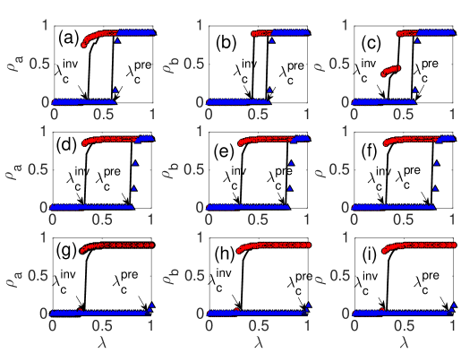
Figure 2 shows the social contagions in the community networks. We find that the final behavior adoption size $\rho_{a}$ in community $a$ increases discontinuously with the information transmission probability $\lambda$, i.e., there is a first-order phase transition that depends on $\rho_{0}$ and $\lambda$. For a small value of the initially adopted seeds $\rho_{0}=0.07$, $\rho_{a}$ increases discontinuously at the presence threshold $\lambda_{c}^{\rm pre}$, i.e., there is a vanishingly small fraction of individuals adopting the behavior when $\lambda\leq\lambda_{c}^{\rm pre}$, and a finite fraction of individuals adopting the behavior when $\lambda>\lambda_{c}^{\rm pre}$.

We find a similar phenomenon for a large seed size $\rho_{0}=0.4$, i.e., $\rho_{b}$ increases discontinuously with $\lambda$ at the invasion threshold $\lambda_{c}^{\rm inv}$. These phenomena indicate that the system exhibits first-order phase transitions with a hysteresis loop. Specifically, the fraction of adopted individuals versus $\lambda$ depends on the initial conditions of $\rho_{0}$ at region $\lambda_{c}^{\rm inv}<\lambda<\lambda_{c}^{\rm pre}$. In this region, for a small fraction of seeds, i.e., $\rho_{0}$ = 0.07, susceptible individuals from both communities are less likely to receive a number of information units that exceeds the adoption threshold. Large values of transmission probability $\lambda$ are needed to accelerate social contagion. When there is a large fraction of initial adopters, i.e., $\rho_{0}=0.4$, the probability that the number of information units received by a susceptible individual exceeds the adoption threshold increases. When the values of the transmission probability $\lambda$ are small, the contagion accelerates. The strength of the community structures does not qualitatively affect the phenomena. Figure 2 shows that our theoretical results agree with the numerical simulation results.

Figure 3: (Color online) Effects of the strength of community structures on social contagions. The final adoption size versus $\mu$ with $\lambda=0.5$ in Figs. (a)–(c), $\lambda=0.7$ in Figs. (d)–(f), $\lambda=0.9$ in Figs. (g)–(i). The three columns respectively represents the final behavior adoption size in community $a$, $b$ and the system. Red circles (blue up triangles) are numerical simulations with $\rho_{0}=0.4$ ($0.07$). The lines are the theoretical predictions. The gray areas in Figs. (e), (f), (h) and (i) represent the optimal community structure that diffuses in global network.

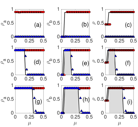
We next determine the effect of community structure $\mu$ under differing initial conditions (see Fig. 3). As in Fig. 2, we find a hysteresis loop phenomenon, i.e., $\rho$ ($\rho_{a}$ or $\rho_{b}$) may have different values under different initial seed sizes. In community $a$, irrespective of the proportion of intercommunity links ($\mu$), the internal connectivity can spread the contagion to the entire originating community $a$ when $\rho_{0}$ is large ($\rho_{0}=0.4$), as shown in Figs. 3(a), 3(d), and 3(g). Figures 3(d) and 3(g) show that increasing $\lambda$, i.e., $\lambda=0.7$ and $\lambda=0.9$, when $\mu$ is small activates the modular structure in the originating community by a small $\rho_{0}$ value. As $\mu$ increases, more intralinks (within communities) are replaced by interlinks (between two communities). When $\mu$ is large, individuals in community $a$ are less likely to expose adopted neighbors. When $\mu$ is increased, the number of susceptible individuals adopting the information in community $a$ decreases. Although susceptible individuals in community $b$ acquire more adopted neighbors in community $a$, their number does not exceed $\theta$. Individuals in community $b$ have no adopted state. Increasing $\mu$ prevents the contagion from spreading to the entire network through internal connectivity. In community $b$ when both $\rho_{0}$ and $\mu$ are small there are insufficient intercommunity bridges to propagate social contagion from community $a$ to community $b$, even when community $a$ is fully saturated [see Figs. 3(e) and 3(h)]. Thus susceptible individuals in community $b$ have too few adopted neighbors in community $a$ to receive information sufficient to exceed the adoption threshold.

Figures 3(e) and 3(h) show that increasing $\mu$ provides the optimal community structure for social contagions. Here the system modularity is sufficiently large to initiate local spreading, sufficiently small to induce intercommunity spreading, and the modular structure allows intercommunity spreading from community $a$ to community $b$. Thus social contagions exist in both communities $a$ and $b$ in this region. If $\mu$ is too large, however, although there are sufficient intercommunity bridges, the system modularity is too small to initiate intercommunity spreading from community $a$. Because the originating community is not saturated, the diffusion does not spread to community $b$ [see Figs. 3(d) and 3(g)]. When $\rho_{0}$ is large ($\rho_{0}=0.4$), the strong community structure enables intercommunity spreading from the originating community $a$ to community $b$. Again our theory agrees with the numerical simulations.

Figure 4: (Color online) Phase diagram of the social contagions on plane $\mu-\lambda$. In (a), (c) and (e), we set $\rho_{0}=0.07$. And in (b), (d) and (f), we set $\rho_{0}=0.4$. The symbols and lines are the numerical and theoretical predictions of the threshold points, respectively. The lines in (a)-(b), (c)-(d) and (e)-(f) represent $\rho_{a}$, $\rho_{b}$ and $\rho$, respectively. Region I (red), II (blue) and III (green) are global diffusion, no diffusion and local diffusion region, respectively.

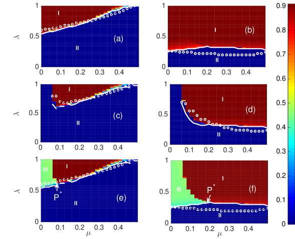
Figure 4 shows the effects of $\lambda$ and $\mu$. Depending on the fraction of the final behavior adoption size, the plane is divided into phase diagrams: global diffusion (region I), no diffusion (region II), and local diffusion (region III). The behavior of $\rho_{\infty}$ as a function of $\mu$ and $\lambda$ exhibits qualitatively different patterns depending on $\rho_{0}$.

When $\mu$ is small, intralinks greatly outnumber interlinks. In response to initially adopted seeds in community $a$, susceptible community $a$ individuals are more likely to become adopted if the number of received information units exceeds threshold $\theta$. When there are fewer interlinks, community $b$ individuals are less likely to receive message units that exceed the threshold, and the social contagion remains local (region III). Increasing $\mu$ enables susceptible community $b$ individuals to receive more message units from exposed adopted neighbors in community $a$. Global diffusion (region I) emerges when the message units that individuals in community $b$ receive exceed threshold $\theta$. When there are few initial adopter seeds, the probability that susceptible individuals have adopter neighbors decreases as the number of intralinks decreases. When the number of adopter seeds is too small to transmit sufficient message units to both communities $a$ and $b$, the no-diffusion area (region II) appears. When the information transmission probability $\lambda$ is too small, the message units received by susceptible individuals in both communities do not exceed $\theta$ and no susceptible individuals adopt the information.

Figure 4(e) shows that when $\rho_{0}=0.07$ is small and community strength is intermediate and finite, $\mu$ allows global spreading. However when $\mu$ is large the number of intracommunity links is too small to propagate spreading in the originating community $a$ and thus cannot be transmitted over the entire system, but when $\rho_{0}=0.4$ is large [see Fig. 4(f)] and larger than the critical value for transition in a system without communities, increasing $\mu$ does not block local spreading, and global diffusion occurs only through external links. We find a rich phase diagram in the $\mu$–$\lambda$ plane with a triple point $P^{*}$. As $\mu$ decreases, the first order transition line that separates global diffusion (region I) from no diffusion (region II) forks into two branches and generates a new local diffusion phase (region III). Around $P^{*}$ a small variform percentage of the edges between the communities can induce an abrupt change in the number of adopted individuals.

5 Conclusions

In this paper we have studied the reinfection pattern that most previous research has ignored. Using infection thresholds we systematically investigate how reinfection affects the social contagion dynamics in community networks. We use a mean-field approximation approach that produces results that agree with numerical simulation results. We find that first-order phase transitions exist during the spreading process in communities, and that a hysteresis loop emerges when the spreading probability at region $\lambda_{c}^{\rm inv}<\lambda<\lambda_{c}^{\rm pre}$ is in the system for different initial adopter densities. We also find an optimal level of community structure strength that facilitates the global diffusion of a small number of initially adopted seeds. In this optimal community structure, global diffusion requires a minimal number of adopters in the community. When the number of links between the communities is decreased, we find a rich phase diagram with a triple point. Our numerical results agree with our proposed mean-field approach, which quantifies, using threshold models, the influence of reinfection in communal networks.

Our results use the initially adopted seeds in only one community. Using numerical simulations and theoretical analyses, we find that our conclusions are not qualitatively affected when the seeds are randomly selected in two communities, and our theory produces results that agree with simulation results when community networks are scale-free. In addition, the amount of heterogeneity in the communal degree distribution does not qualitatively affect these phenomena. Our findings enrich our understanding of how social contagions transmit through communal systems. Our theory in this work can be used to study epidemic spreading [46, 6, 47, 48], the effects of vaccination [49], and the impact of human behavior [50, 51] on epidemics. In future work we will further explore our approach using real social contagion data.

References

- [1] Castellano C, Fortunato S, Loreto V 2009 Rev. Mod. Phys. 81 591.
- [2] Boccaletti S, Latora V, Moreno Y, Chavez M and Hwang D U 2006 Phys. Rep. 424 175.
- [3] Guardiola X, Daz-Guilera A, Perez C J, Arenas A, and Llas M 2002 Phys. Rev. E 66 026121.
- [4] Ohta H and Sasa S 2010 EPL 90 27008.
- [5] Pastor-Satorras R, Castellano C, Van Mieghem P, et al. 2014. Rev. Mod. Phys. 87(3)120-131.
- [6] Li D, Qin P, Wang H, et al. 2014 Europhys. Lett. 105(6) 68004-68008(5).
- [7] Wang W, Tang M, Stanley H E and Braunstein L A 2017 Rep. Prog. Phys. 80 036603.
- [8] Pastor-Satorras R, Castellano C, Van Mieghem P 2015 Rev. Mod. Phys. 87 925.
- [9] Su Z, Wang W, Li L, et al. 2017 Sci. Rep. 7(1):6103.
- [10] Gao J, Buldyrev S V, Stanley H E, et al. 2012 Nat. Phys. 8(1):40-48.
- [11] Watts D J 2002 PNAS 99 5766-5771.
- [12] D. Centola 2011 Science 334 1269.
- [13] A. Banerjee, A. G. Chandrasekhar, E. Duflo, and M. O. Jackson Science 341 363.
- [14] Lee E, Holme P. 2017 Phys. Rev. E 96(1): 012315.
- [15] Wang W, Tang M, Shu P and Wang Z 2016 New J. Phys. 18 013029.
- [16] Pastor-Satorras, R., Castellano, C., Van, M. P. Vespignani, A 2015 Rev. Mod. Phys. 87 925.
- [17] Castellano, C., Fortunato, S. Loreto, V. 2009 Rev. Mod. Phys. 81 591.
- [18] Dorogovtsev, S. N., Goltsev, A. V. Mendes, J. F. 2008 Rev. Mod. Phys. 80 1275.
- [19] J. P. Gleeson and D. J. Cahalane 2007 Phys. Rev. E 75 056103.
- [20] D. E. Whitney 2010 Phys. Rev. E 82 066110.
- [21] J. P. Gleeson 2008 Phys. Rev. E 77 046117.
- [22] A. Nematzadeh, E. Ferrara, A. Flammini, and Y.-Y. Ahn 2014 Phys. Rev. Lett. 113 088701.
- [23] K.-M. Lee, C. D. Brummitt, and K.-I. Goh 2014 Phys. Rev. E 90 062816.
- [24] C. D. Brummitt, K.-M. Lee, and K.-I. Goh 2012 Phys. Rev. E 85 045102(R).
- [25] Wang W, Stanley H E, Braunstein L A. 2018 New J. Phys. 20 013034
- [26] Boccaletti S, Bianconi G, Criado R, et al. 2014 Phys. Rep. 544(1) 1-122.
- [27] Wang Z, Wang L, Szolnoki A, et al. 2015 Eur. Phys. J. B 88(5) 124.
- [28] Lee K M, Brummitt C D, Goh K I 2014 Phys. Rev. E 90(6) 062816.
- [29] Brummitt C D, Lee K M, Goh K I 2012 Phys. Rev. E 85(4) 045102.
- [30] Yaan O, Gligor V. 2012 Phys. Rev. E 86(3) 036103.
- [31] Takaguchi T, Masuda N, Holme P. 2013 PloS one,8(7) e68629.
- [32] Karimi, F., Holme, P 2013 Physica A, 392(16) 3476-3483.
- [33] Wang W, Tang M, Zhang H F, et al. 2015 Phys. Rev. E 92(1) 012820.
- [34] Wang W, Tang M, Shu P, et al. 2016 New J. Phys. 18(1) 013029.
- [35] Radicchi F 2014 Phys. Rev. X 4 021014.
- [36] Dodds P S, Payne J L 2009 Phys. Rev. E 79(6): 066115.
- [37] Nematzadeh A, Ferrara E, Flammini A and Ahn Y Y 2014 Phys. Rev. Lett. 113 088701.
- [38] Majdandzic A, Podobnik B, Buldyrev S V, et al. 2014 Nat. Phys. 10(1) 34-38.
- [39] Dodds P S, Watts D J 2004 Phys. Rev. Lett. 92(21) 0031-9007.
- [40] Pastor-Satorras R, Castellano C, Van Mieghem P, et al. 2015 Rev. Mod. Phys. 87(3): 925.
- [41] Liu M X, Wang W, Liu Y, Tang M, Cai S M and Zhang H F 2017 Phys. Rev. E 95 052306.
- [42] Pastor-Satorras R, Vespignani A 2001 Phys. Rev. Lett. 86(14):3200-3.
- [43] Newman M E J, Reinert G. 2016 Phys. Rev. Lett. 117(7): 078301.
- [44] Newman M E J, Peixoto T P. 2015 Phys. Rev. Lett. 115(8): 088701.
- [45] Gao J, Barzel B, and Barabsi A L 2016 Nature, 530 307-312.
- [46] Domenico M D, Granell C, Porter M A, et al. 2016 Nat. Phys. 12(10) 901-906.
- [47] Wang Z, Andrews M A, Wu Z X, et al. 2015 Phys. Life Rev., 15 1-29.
- [48] Wang Z, Moreno Y, Boccaletti S, et al. 2017 Chaos Soliton. Fract. 103 177-183.
- [49] Wang Z, Bauch C T, Bhattacharyya S, et al. 2016 Phys. Rep. 664.
- [50] Li X, Jusup M, Wang Z, et al. 2018 Proc. Natl. Acad. Sci. 115(1) 30.
- [51] Wang Z, Jusup M, Wang R, et al. 2017 Science Adv. 3(3) e1601444.