Sample-to-Sample Correspondence for Unsupervised Domain Adaptation

Abstract

The assumption that training and testing samples are generated from the same distribution does not always hold for real-world machine-learning applications. The procedure of tackling this discrepancy between the training (source) and testing (target) domains is known as domain adaptation. We propose an unsupervised version of domain adaptation that considers the presence of only unlabelled data in the target domain. Our approach centers on finding correspondences between samples of each domain. The correspondences are obtained by treating the source and target samples as graphs and using a convex criterion to match them. The criteria used are first-order and second-order similarities between the graphs as well as a class-based regularization. We have also developed a computationally efficient routine for the convex optimization, thus allowing the proposed method to be used widely. To verify the effectiveness of the proposed method, computer simulations were conducted on synthetic, image classification and sentiment classification datasets. Results validated that the proposed local sample-to-sample matching method out-performs traditional moment-matching methods and is competitive with respect to current local domain-adaptation methods.

1 Introduction

In traditional machine-learning settings, we assume that the testing data belongs to the same distribution as the training data. However, such an assumption is rarely encountered in real-world situations. For example, consider a recognition system that distinguishes between a cat and a dog, given labelled training samples of the type shown in Fig. 1(a). These training samples are frontal faces of cats and dogs. When the same recognition system is used to test in a different domain such as on the side images of cats and dogs as shown in Fig. 1(b), it would fail miserably. This is because the recognition system has developed a bias in being able to only distinguish between the face of a dog and a cat and not side images of dogs and cats. Domain adaptation (DA) aims to mitigate this dataset bias [46], where different datasets have their own unique properties.

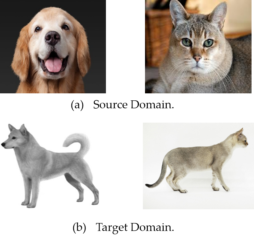
Figure 1: Discrepancy between the source domain and the target domain. In the source domain, the images have frontal faces while the target domain has images of the whole body from the side view-point.

Dataset bias appears because of the distribution shift of data from one dataset (i.e., source domain) to another dataset (i.e., target domain). The distribution shift manifests itself in different forms. In computer vision, it can occur when there is changing lighting conditions, changing poses, etc. In speech processing, it can be due to changing accent, tone and gender of the person speaking. In remote sensing, it can be due to changing atmospheric conditions, change in acquisition devices, etc. To encounter this discrepancy in distributions, domain adaptation methods have been proposed. Once domain adaptation is carried out, a model trained using the adapted source domain data should perform well in the target domain. The underlying assumption in domain adaptation is that the task is the same in both domains. For classification problems, it implies that we have the same set of categories in both source and target domains.

Domain adaptation can also assist in annotating datasets efficiently and further accelerating machine-learning research. Current machine-learning models are data hungry and require lots of labelled samples. Though huge amount of unlabelled data is obtained, labelling them requires lot of human involvement and effort. Domain adaptation seeks to automatically annotate unlabelled data in the target domain by adapting the labelled data in the source domain to be close to the unlabeled target-domain data.

In our work, we consider unsupervised domain adaptation (UDA), which assumes absence of labels in the target domain. This is more realistic than semi-supervised domain adaptation, where there are also a few-labelled data in the target domain. This is because labelling data might be time-consuming and expensive for real-world situations. Hence we need to effectively exploit fully labelled source-domain data and fully unlabelled target-domain data to carry out domain adaptation. In our case, we seek to find correspondences between each source-domain sample and each target-domain sample. Once the correspondences are found, we can transform the source-domain samples to be close to the target-domain samples. The transformed source-domain samples will then lie close to the data space of the target domain. This will allow a model trained on the transformed source-domain data to perform well with the target-domain data. This not only achieves the goal of training robust models but also allows the model to annotate unlabelled target-domain data accurately.

The remainder of the paper is organized as follows: Section 2 discusses related work of domain adaptation. Section 3 discusses the background required for our proposed approach. Section 4 discusses our proposed approach and formulates our unsupervised domain adaptation problem into a constrained convex optimization problem. Section 5 discusses the experimental results and some comparison with existing work. Section 6 discusses some limitations. Section 7 concludes with a summary of our work and future research directions. Finally, the Appendix shows more details about the proof of convexity of the optimization objective function and derivation of the gradients.

2 Related Work

There is a large body of prior work on domain adaptation. For our case, we only consider homogeneous domain adaptation, where both the source and target domains have the same feature space. Most of previous DA methods are classified into two categories, depending on whether a deep representation is learned or not. In that regard, our proposed approach is not deep-learning-based since we directly work at the feature level without learning a representation. We feel that our method can easily be extended to deep architectures and provide much better results. For a comprehensive overview on domain adaptation, please refer to Csurka’s survey paper [11].

2.1 Non-Deep-Learning Domain-Adaptation Methods

These non-deep-learning domain-adaptation methods can be broadly classified into three categories – instance re-weighting methods, parameter adaptation methods, and feature transfer methods. Parameter adaptation methods [31, 7, 14, 50] generally adapt a trained classifier in the source domain (e.g., an SVM) in order to perform better in the target domain. Since these methods require at least a small set of labelled target examples, they cannot be applied to UDA.

Instance Re-weighting was one of the early methods, where it was assumed that conditional distributions were shared between the two domains. The instance re-weighting involved estimating the ratio between the likelihoods of being a source example or a target example to compute the weight of an instance. This was done by estimating the likelihoods independently [51] or by approximating the ratio between the densities [32, 43]. One of the most popular measures used to weigh data instances, used in [26, 29], was the Maximum Mean Discrepancy (MMD) [5] calculated between the distributions in different domains. Feature Transfer methods, on the other hand, do not assume the same conditional distributions between the source and target domains. An early method for Domain Adaptation was proposed in [12], where the representation is modifed such that the source features are $({\bf x}_{s},{\bf x}_{s},0)$ and the target features are $({\bf x}_{t},0,{\bf x}_{t})$. This enables identifying shared and domain-specific features. Other ideas include the Geodesic Flow Sampling (GFS) [25, 24] and the Geodesic Flow Kernel (GFK) [23, 22], where the domains are considered as samples on the Grassman manifolds. The Subspace Alignment (SA) [17] method aligns source and target domain subspaces using Bregman divergence. The linear Correlation Alignment (CORAL) [44] algorithm aligns the source and target data covariances. Transfer Component Analysis (TCA) [39] discovers shared hidden features having simmilar distribution between the two domains. Chen at al.[8] proposed a reconstruction based approach to learn a domain invariant representation. Most of these previous methods learned global alignment between the two domains. On the other hand, the Adaptive Transductive Transfer Machines (ATTM) [16] and Optimal Transport [10] considers sample to sample alignment between the source and target distributions.

2.2 Deep Domain-Adaptation Methods

Most deep-learning methods for DA use a siamese architecture with two streams for the source and target domain. These methods use classification loss in addition to a discrepancy loss [36, 34, 48, 21, 45] or an adversarial loss. The classification loss depends on the labelled source data, and the discrepancy loss diminishes the shift between the two domains. On the other hand, adversarial-based methods play a game of generating domain-invariant representations with the domain discriminator. Tzeng et al. [47] proposes a unified view of existing adversarial DA methods by comparing them according to the loss type, the weight-sharing strategy between the two streams, and on whether they are discriminative or generative. The Domain-Adversarial Neural Networks (DANN) [19] used a gradient reversal layer to produce features that are discriminative as well as domain-invariant. The main disadvantage of these adversarial methods is that their training is generally not stable. Moreover, empirically tuning the capacity of a discriminator requires lot of effort.

Between these two classes of DA methods, the state-of-the-art methods are dominated by deep architectures. However, these approaches are quite complex and expensive, requiring re-training of the network and tuning of many hyper parameters such as the structure of the hidden adaptation layers. Non-deep-learning domain-adaptation methods do not achieve as good performance as a deep-representation approach, but they work directly with shallow/deep features and require lesser number of hyper-parameters to tune. Among the non-deep-learning domain-adaptation methods, we feel feature transformation methods are more generic because they directly use the feature space from the source and target domains, without any underlying assumption of the classification model. In fact, a powerful shallow-feature transformation method can be extended to deep-architecture methods, if desired, by using the features of each and every layer and then jointly optimizing the parameters of the deep architectures as well as that of the classification model. For example, correlation alignment [44] has been extended for deep architectures [45], which evidently achieve the state-of-the art performance. Moreover, we believe a local transformation-based approach as in [10, 16] will result in better performance than global transformation methods because it considers the effect of each and every sample in the dataset explicitly.

3 Background

Our local transformation-based approach to DA places a strong emphasis on establishing a sample-to-sample correspondence between each source-domain sample and each target-domain sample. Establishing correspondences between two sets of visual features have long been used in computer vision mostly for image registration [3, 9]. To our knowledge, the approach of finding correspondences between the source-domain and the target-domain samples has never been used for domain adaptation. The only work that is similar to finding correspondences is the work on optimal transport [10]. They learned a transport plan for each source-domain sample so that they are close to the target-domain samples. Their transport plan is defined on a point-wise unary cost between each source sample and each target sample. Our approach develops a framework to find correspondences between the source and target domains that exploit higher-order relations beyond these unary relations between the source and target domains. We treat the source-domain data and the target-domain data as the source and target hyper-graphs, respectively, and our correspondence problem can be cast as a hyper-graph matching problem. The hyper-graph matching problem has been previously used in computer vision [15] through a tensor-based formulation but has not been applied to domain adaptation. Hyper-graph matching involves using higher-order relations between samples such as unary, pairwise, tertiary or more. Pairwise matching involves matching source-domain sample pairs with target-domain sample pairs. Tertiary matching involves matching source-domain sample triplets with target-domain sample triplets and so on. Thus, hyper-graph methods provide additional higher-order geometric and structural information about the data that is missing with just using unary point-wise relations between a source sample and a target sample.

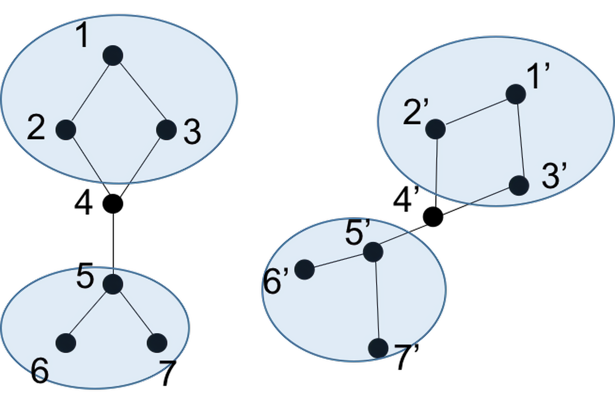
Figure 2: Example showing the advantage of higher-order graph matching compared to just first-order matching.

The advantage of using higher-order information in graph matching is demonstrated in the example in Fig. 2. In Fig. 2, the graph on the left is constructed from the source domain while the graph on the right is constructed from the target domain. In the graph, each node represents a sample and edges represent connectivity among the samples. Among these, samples $1$ and $1^{\prime}$ do not match because those samples are not the closest pair of samples. But as a group $\{1,2,3\}$ matches with $\{1^{\prime},2^{\prime},3^{\prime}\}$ suggesting that higher-order matching can aid domain adaptation, whereas one-to-one matchings between samples might not provide enough or provide incorrect information. Unfortunately, higher-order graph matching comes with increasing computational complexity and also extra hyper-parameters that weigh the importance of each of the higher-order relations. Therefore , in our work we consider only the first-order and second-order matchings to validate the approach. Still, our problem can be inefficient because the number of correspondence variables increases with the number of samples. To address all these problems, we contribute in the following ways:

1. We initially propose a mathematical framework that uses the first-order and second-order relations to match the source-domain data and the target-domain data. Once the relations are established, the source domain is mapped to be close to the target domain. A class-based regularization is also used to leverage the labels present in the source domain. All these cost factors are combined into a convex optimization framework.

2. The above transformation approach is computationally inefficient. We then reformulate our convex optimization problem into solving a series of sub-problems for which an efficient solution using a network simplex approach. This new formulation is more efficient in terms of both time and storage space.

3. Finally, we have performed experimental evaluation of our proposed method on both toy datasets as well as real image and sentiment classification datasets. We have also examined the effect of each cost term in the convex optimization problem separately.

The overall scheme of our proposed approach is shown in Fig. 3

Figure 3: Conceptual and high-level description of our proposed convex optimization formulation with its proposed solution. The inputs are source-domain data (${\bf X}^{s}$), source-domain labels (${\bf Y}^{s}$), and target-domain data (${\bf X}^{t}$). Output is a mapping function (${\bf M}(\cdot)$) that maps ${\bf X}^{s}$ close to ${\bf X}^{t}$. The transformation can be repeated again by providing the transformed source data ${\bf M}({\bf X}^{s})$, source labels ${\bf Y}^{s}$ and target data ${\bf X}^{t}$ as input.

4 Proposed Sample-to-Sample Correspondence Method

In this section, we shall first define the domain adaptation problem [40, 49], and then formulate the proposed correspondence-and-mapping method for the unsupervised domain adaptation problem.

4.1 Notation

A domain consists of a $d$-dimensional feature space $\mathcal{X}\subset\mathbb{R}^{d}$ with a marginal probability distribution $P({\bf X})$. The task $\mathcal{T}$ is defined using a label space $\mathcal{Y}$ and the conditional probability distribution $P({\bf Y}|{\bf X})$. Here ${\bf X}$ and ${\bf Y}$ are random variables. For a particular sample set ${\bf X}=\{{\bf x}_{1},\ldots,{\bf x}_{n}\}$ of $\mathcal{X}$ with labels ${\bf Y}=\{{y}_{1},\ldots,{y}_{n}\}$ from $\mathcal{Y}$, $P({\bf Y}|{\bf X})$ can be trained in a supervised way from feature and labels $\{{\bf x}_{i},y_{i}\}$. For the domain adaptation purpose, we assume that there are two domains with the same task: a source domain $\mathcal{D}^{s}=\{\mathcal{X}^{s},P({\bf X}^{s})\}$ with $\mathcal{T}^{s}=\{\mathcal{Y}^{s},P({\bf Y}^{s}|{\bf X}^{s})\}$ and a target domain $\mathcal{D}^{t}=\{\mathcal{X}^{t},P({\bf X}^{t})\}$ with $\mathcal{T}^{t}=\{\mathcal{Y}^{t},P({\bf Y}^{t}|{\bf X}^{t})\}$. Traditional machine learning techniques assume that both $\mathcal{D}^{s}=\mathcal{D}^{t}$ and $\mathcal{T}^{s}=\mathcal{T}^{t}$, where $\mathcal{D}^{s}$ becomes the training set and $\mathcal{D}^{t}$ the test set. For domain adaptation, $\mathcal{D}^{t}\neq\mathcal{D}^{s}$ but $\mathcal{T}^{t}=\mathcal{T}^{s}$. When the source domain is related to the target domain, it is possible to use the relational information from ${\mathcal{D}^{s},\mathcal{T}^{s}}$ to learn $P({\bf Y}^{t}|{\bf X}^{t})$. The presence/absence of labels in the target domain also decide how domain adaptation is being carried out. We shall solve the most challenging case, where we have labelled source domain data but unlabeled data in the target domain. This is commonly known as unsupervised domain adaptation (UDA). A natural extension to UDA is the semi-supervised case, where a small set of target domain samples is labelled.

In our case, we have labelled source-domain data with a set of training data ${\bf X}^{s}=\{{\bf x}^{s}_{i}\}^{n_{s}}_{i=1}$ associated with a set of class labels ${\bf Y}^{s}=\{y^{s}_{i}\}^{n_{s}}_{i=1}$. In the target domain, we only have unlabelled samples ${\bf X}^{t}=\{{\bf x}^{t}_{i}\}^{n_{t}}_{i=1}$. If we had already trained a classifier using the source-domain samples, the performance of the target-domain samples on that classifier would be quite poor. This is because the distributions of the source and target samples are different; that is, $P({\bf X}^{s})\neq P({\bf X}^{t})$. So we need to to find a transformation of the input space ${\bf F}:\mathcal{X}^{s}\rightarrow\mathcal{X}^{t}$ such that $P(y|{\bf x}^{t})=P(y|{\bf F}({\bf x}^{s}))$. As a result of this transformation, the classifier learned on the transformed source samples can perform satisfactorily on the target-domain samples.

4.2 Correspondence-and-Mapping Problem Formulation

With the above notation, our proposed approach considers the transformation ${\bf F}$ as a point-set registration between two point sets, where the source samples $\{{\bf x}^{s}_{i}\}^{n_{s}}_{i=1}$ are the moving point set and the target samples $\{{\bf x}^{t}_{i}\}^{n_{t}}_{i=1}$ are the fixed point set. In such a case, the registration involves alternately finding the correspondence and mapping between the fixed and moving point sets [9, 3]. The advantage of point-set registration is that it ensures explicit sample-to-sample matching and not moment matching like covariance in CORAL [44] or MMD [36, 34, 48, 21]. As a result, the transformed source domain matches better with the target domain. However, matching each and every sample requires an optimizing variable for each pair of source and target domain samples. If the number of samples increases, so does the number of variables and the optimization procedure may become extremely costly. We shall discuss how to deal with the computational inefficiency later.

For the case when the number of target samples equals to the number of source samples; that is, $n_{t}=n_{s}$, the correspondence can be represented by a permutation matrix ${\bf P}\in\{0,1\}^{n_{s}\times n_{t}}$. Element $[{\bf P}]_{ij}=1$ if the source-domain sample ${\bf x}^{s}_{i}$ corresponds to the target-domain sample ${\bf x}^{t}_{j}$, and 0, otherwise. The permutation matrix ${\bf P}$ has constraints $\sum_{i}[{\bf P}]_{ij}=1$ and $\sum_{j}[{\bf P}]_{ij}=1$ for all $i\in\{1,2,\ldots,n_{s}\}$ and $j\in\{1,2,\ldots,n_{t}\}$. Hence, if ${\bf X}^{s}\in\mathbb{R}^{n_{s}\times d}$ and ${\bf X}^{t}\in\mathbb{R}^{n_{t}\times d}$ be the data matrix of the source-domain and the target-domain data, respectively, then ${\bf P}{\bf X}^{t}$ permutes the target-domain data matrix.

As soon as the correspondence is established, a linear or a non-linear mapping must be established between the target samples and the corresponding source samples. Non-linear mapping is involved when there is localized mapping for each sample, and it might also be required in case there is unequal domain shift of each class. The mapping operation should map the source-domain samples as close as possible to the corresponding target-domain samples. This process of finding a correspondence between these transformed source samples and target samples and then finding the mapping will continue iteratively till convergence. This iterative method of alternately finding the correspondence and mapping is similar to feature registration in computer vision [9, 3] but they have not been used or reformulated for unsupervised domain adaptation . In fact, the feature registration methods formulate the problem as a non-convex optimization. Consequently, these methods suffer from local minimum as in [3], and the global optimization technique such as deterministic annealing [9] does not guarantee convergence. Thus, we propose to formulate it as a convex optimization problem to obtain correspondences as a global solution. It is important to note that finding such global and unique solution to the correspondence accurately is more important because mapping with inaccurate correspondences will undoubtedly yield bad results.

Formulating the proposed unsupervised domain adaptation problem as a convex optimization problem requires the correspondences to have the following properties: (a) First-order similarity: The corresponding target-domain samples should be as close as possible to the corresponding source-domain samples. This implies that we want to have the permuted target-domain data matrix ${\bf P}{\bf X}^{t}$ to be close to the source-domain data matrix ${\bf X}^{s}$, which translates to minimizing the Frobenius norm $||{\bf P}{\bf X}^{t}-{\bf X}^{s}||^{2}_{\mathcal{F}}$ in the least-squares sense . (b) Second-order similarity: The corresponding target-domain neighborhood should be structurally similar to the corresponding source-domain neighborhood. This structural similarity can be expressed using graphs constructed from the source and target domains. Thus, if the two domains can be thought of as weighted undirected graphs $G^{s},G^{t}$, structural similarity implies matching edges between the source and the target graphs. The edges of these graphs can be expressed using the adjacency matrices. If ${\bf D}^{s}$ and ${\bf D}^{t}$ are the adjacency matrices of $G^{s}$ and $G^{t}$, respectively, then these adjacency matrices can be found as,

$$[{\bf D}^{s}]_{ij}=\text{exp}({-\frac{||{\bf x}^{s}_{i}-{\bf x}^{s}_{j}||^{2}_{2}}{{\sigma}_{s}^{2}}})$$

$$[{\bf D}^{t}]_{ij}=\text{exp}({-\frac{||{\bf x}^{t}_{i}-{\bf x}^{t}_{j}||^{2}_{2}}{{\sigma}_{t}^{2}}})$$

$$[{\bf D}^{s}]_{ii}=[{\bf D}^{t}]_{ii}=0,$$

where ${\sigma}_{s}$ and ${\sigma}_{t}$ can be found heuristically as the mean sample-to-sample pairwise distance in the source and target domains, respectively. For the second-order similarity, we want the permuted target domain adjacency matrix ${\bf P}{\bf D}^{t}{\bf P}^{T}$ to be close to the source domain adjacency matrix (region) ${\bf D}^{s}$, where the superscript $T$ indicates a matrix transpose operation. We formulate it as equivalent to minimizing $||{\bf P}{\bf D}^{t}{\bf P}^{T}-{\bf D}^{s}||^{2}_{\mathcal{F}}$. While this cost term geometrically implies the cost of mis-matching edges in the constructed graphs, the first-order similarity term can be thought as the cost of mis-matching nodes. However, the second-order similarity cost term is bi-quadratic and we want to make it quadratic so that the cost-function is convex and we can apply convex optimization techniques to it. This can be done by post-multiplying ${\bf P}{\bf D}^{t}{\bf P}^{T}-{\bf D}^{s}$ by ${\bf P}$. Using the permutation matrix properties ${\bf P}^{T}{\bf P}={\bf I}$ (orthogonal) and $||{\bf A}{\bf P}||=||{\bf A}||$ (norm-preserving), this transformation produces the cost function $||{\bf P}{\bf D}^{t}-{\bf D}^{s}{\bf P}||^{2}_{\mathcal{F}}$.

Estimating the correspondence as a permutation matrix in this quadratic setting is NP-hard because of the combinatorial complexity of the constraint on ${\bf P}$. We can relax the constraint on the correspondence matrix by converting it from a discrete to a continuous form. The norms (i.e., Frobenius) used in the cost/regularization terms will yield a convex minimization problem if we replace ${\bf P}$ with a continuous constraint. Hence, if we relax the constraints on ${\bf P}$ to allow for soft correspondences (i.e., replacing ${\bf P}$ with ${\bf C}$), then an element of ${\bf C}$ matrix, $[{\bf C}]_{ij}$, represents the probability that ${\bf x}^{s}_{i}$ corresponds to ${\bf x}^{t}_{j}$. This matrix ${\bf C}$ is called doubly stochastic matrix $\mathcal{D}_{B}=\{{\bf C}\geq{\bf 0}:{\bf C}\mathbf{1}={\bf C}^{T}\mathbf{1}=\mathbf{1}\}$ . $\mathcal{D}_{B}$ represents a convex hull, containing all permutation matrices at its vertices. (Birkhoff-von-Neumann theorem).

In addition to the graph-matching terms, we add a class-based regularization to the cost function that exploits the labelled information of source-domain data. The group-lasso regularizer $\ell_{2}-\ell_{1}$ norm term is equal to $\sum_{j}\sum_{c}||[{\bf C}]_{\mathcal{I}_{c}j}||_{2}$, where $||\cdot||_{2}$ is the $\ell_{2}$ norm and $\mathcal{I}_{c}$ contains the indices of rows of ${\bf C}$ corresponding to the source-domain samples of class $c$. In other words, $[{\bf C}]_{\mathcal{I}_{c}j}$ is a vector consisting of elements $[{\bf C}]_{ij}$, where $i^{th}$ source sample belongs to class $c$ and the $j^{th}$ sample is in the target domain. Minimizing this group-lasso term ensures that a target-domain sample only corresponds to the source-domain samples that have the same label.

It is important to note that the solution to the relaxed problem may not be equal or even close to the original discrete problem. Even then, the solution of the relaxed problem need not be projected onto the set of permutation matrices to get our final solution. This is because the graphs constructed using the source samples and the target samples are far from isomorphic for real datasets. Therefore, we do not expect exact matching between the nodes (samples) of each graph (domain) and soft correspondences may serve better. As an example, consider that a source sample ${\bf x}^{s}_{i}$ is likely to correspond to both ${\bf x}^{t}_{j}$ and ${\bf x}^{t}_{k}$. In that case, it is more appropriate to have correspondences $[{\bf C}]_{ij}=0.7$ and $[{\bf C}]_{ik}=0.3$ assigned to the target samples, rather than the exact correspondences $[{\bf C}]_{ij}=1$ and $[{\bf C}]_{ik}=0$ or vice-versa. Thus, we can formulate our optimization problem of obtaining ${\bf C}$ as follows:

$$\min\limits_{{\bf C}}f({\bf C})= ||{\bf C}{\bf X}^{t}-{\bf X}^{s}||^{2}_{\mathcal{F}}/(n_{s}d)+$$ (1)

$$\lambda_{s}||{\bf C}{\bf D}^{t}-{\bf D}^{s}{\bf C}||^{2}_{\mathcal{F}} +\lambda_{g}\sum_{j}\sum_{c}||[{\bf C}]_{\mathcal{I}_{c}j}||_{2}$$

$${\rm such~{}that~{}}~{}{\bf C}\geq{\bf 0}, ~{}{\bf C}\mathbf{1}_{n_{t}}=\mathbf{1}_{n_{s}},~{}{\rm and}~{}{\bf C}^{T}\mathbf{1}_{n_{s}}=\mathbf{1}_{n_{t}},$$

where $\lambda_{s}$ and $\lambda_{g}$ are the parameters weighing the second-order similarity term and class-based regularization term, respectively; $\mathbf{1}_{n_{s}}$ and $\mathbf{1}_{n_{t}}$ are column vectors of size $n_{s}$ and $n_{t}$, respectively, and the superscript $T$ indicates a matrix transpose operation. The assumption that $n_{t}=n_{s}$ is strict and it needs to be relaxed to allow more realistic situations such as $n_{t}\neq n_{s}$. To analyze what modification is required to the optimization problem in Eq. (1), we explore further to understand the correspondences properly. In the case of $n_{t}=n_{s}$, we have one-to-one correspondences between each source sample and each target sample. However, for the case $n_{t}\neq n_{s}$, we must allow multiple correspondences. Initially, the constraint ${\bf C}\mathbf{1}_{n_{t}}=\mathbf{1}_{n_{s}}$ implies that the sum of the correspondences of all the target samples to each source sample is one. The second equality constraint ${\bf C}^{T}\mathbf{1}_{n_{s}}=\mathbf{1}_{n_{t}}$ implies that the sum of correspondences of all the source samples to each target sample is one. However, if $n_{t}\neq n_{s}$, the sum of correspondences of all the source samples to each target sample should increase proportionately by $\frac{n_{s}}{n_{t}}$ to allow for the multiple correspondences. This is reflected in the following optimization problem.

Problem UDA

$$\min\limits_{{\bf C}}f({\bf C}) =||{\bf C}{\bf X}^{t}-{\bf X}^{s}||^{2}_{\mathcal{F}}/(n_{s}d)+\lambda_{s}||{\bf C}{\bf D}^{t}-(\frac{n_{t}}{n_{s}}){\bf D}^{s}{\bf C}||^{2}_{\mathcal{F}}$$ (2)

$$\quad+\lambda_{g}\sum_{j}\sum_{c}||[{\bf C}]_{\mathcal{I}_{c}j}||_{2}$$

$${\rm such~{}that}~{}{\bf C}\geq{\bf 0},~{}{\bf C}\mathbf{1}_{n_{t}} =\mathbf{1}_{n_{s}},~{}{\rm and}~{}{\bf C}^{T}\mathbf{1}_{n_{s}}=(\frac{n_{s}}{n_{t}})\mathbf{1}_{n_{t}}$$

for $n_{t}\neq n_{s}$.

4.3 Correspondence-and-Mapping Problem Solution

Problem UDA is a constrained convex optimization problem and can easily be solved by interior-point methods [6]. In general, the time complexity of these interior-point-methods for conic programming is $O(N^{3.5})$, where $N$ is the total number of the variables [1]. If we have $n_{s}$ and $n_{t}$ as source and target samples, respectively, then the time complexity becomes $O(n_{s}^{3.5}n_{t}^{3.5})$. Also, the interior-point method is a second-order optimization method. Hence, it requires storage space of the Hessian, which is $O(N^{2})$ $\sim$ $O(n_{s}^{2}n_{t}^{2})$. This space complexity is more alarming and does not scale well with an increasing number of variables. If $n_{t}$ and $n_{s}$ are greater than 100 points, it results in memory/storage-deficiency problems in most personal computers. Thus, we need to employ a different optimization procedure so that the proposed UDA approach can be widely used without memory-deficiency problem. We could think of first-order methods of solving the constrained optimization problem, which require computing gradients but do not require storing the Hessians.

First-order methods of solving the constrained optimization problem can be broadly classified into projected-gradient methods and conditional gradient (CG) methods [18]. The projected-gradient method is similar to the normal gradient-descent method except that for each iteration, the iterate is projected back into the constraint set. Generally, the projected gradient-descent method enjoys the same convergence rate as the unconstrained gradient-descent method. However, for the projected gradient-descent method to be efficient, the projection step needs to be inexpensive. With an increasing number of variables, the projection step can become costly. Furthermore, the full gradient updating may destroy the structure of the solutions such as sparsity and low rank. The conditional gradient method, on the other hand, maintains the desirable structure of the solution such as sparsity by solving the successive linear minimization sub-problems over the convex constraint set. Since we expect our correspondence matrix ${\bf C}$ to be sparse, we shall employ the conditional gradient method for our problem. In fact, Jaggi [30] points out that convex optimization problems over convex hulls of atomic sets, which are relaxations of NP-hard problems are directly suitable for the conditional gradient method. This is similar to the way we formulate our problem by relaxing ${\bf P}$ matrix to ${\bf C}$.

Given : ${\bf C}_{0}\in\mathcal{D}$, $t=1$

Repeat

 ${\bf C}_{d}=\text{arg}\min\limits_{{\bf C}}\text{Tr}(\nabla_{C}f({\bf C}_{0})^{T}{\bf C}),\quad\text{such that}\quad{\bf C}\in\mathcal{D}$

 ${\bf C}_{1}={\bf C}_{0}+\alpha({\bf C}_{d}-{\bf C}_{0}),\quad\text{for}\quad\alpha=\frac{2}{t+2}$

 ${\bf C}_{0}={\bf C}_{1}$  and  $t=t+1$

Until Convergence or Fixed Number of Iterations

Output : ${\bf C}_{0}=\text{arg}\min\limits_{{\bf C}}f({\bf C})\quad\text{such that}\quad{\bf C}\in\mathcal{D}$

Algorithm 1 Conditional Gradient Method (CG).

As described in the above Algorithm 1 of the conditional gradient method, we have to solve the linear programming problem, $\min\limits_{{\bf C}}\text{Tr}(\nabla_{C}f({\bf C}_{0})^{T}{\bf C})$, such that ${\bf C}\in\mathcal{D}=\{{\bf C}:{\bf C}\geq{\bf 0},{\bf C}\mathbf{1}_{n_{t}}=\mathbf{1}_{n_{s}},{\bf C}^{T}\mathbf{1}_{n_{s}}=(\frac{n_{s}}{n_{t}})\mathbf{1}_{n_{t}}\}$. Here $\text{Tr}(\cdot)$ is the Trace operator. The gradient $\nabla_{\bf C}f$ can be found from the equation:

$$\ \nabla_{\mathbf{C}}f=\nabla_{\mathbf{C}}f_{1}/(n_{s}d)+\lambda_{s}\nabla_{\mathbf{C}}f_{2}+\lambda_{g}\nabla_{\mathbf{C}}f_{3},$$ (3)

where $f_{1}$, $f_{2}$, and $f_{3}$ are $||{\bf C}{\bf X}^{t}-{\bf X}^{s}||^{2}_{\mathcal{F}}$, $||{\bf C}{\bf D}^{t}-(\frac{n_{t}}{n_{s}}){\bf D}^{s}{\bf C}||^{2}_{\mathcal{F}}$, and $\sum_{j}\sum_{c}||[{\bf C}]_{\mathcal{I}_{c}j}||_{2}$, respectively.

The gradients are obtained as follows. The derivation is given in the Appendix section-

$$\nabla_{\mathbf{C}}f_{1}=2({\bf C}{\bf X}^{t}-{\bf X}^{s})({\bf X}^{t})^{T}$$

$$\nabla_{\mathbf{C}}f_{2}=2{\bf C}{\bf D}^{t}({\bf D}^{t})^{T}-2r{\bf D}^{s}{\bf C}({\bf D}^{t})^{T}-2r({\bf D}^{s})^{T}{\bf C}{\bf D}^{t}+2r^{2}({\bf D}^{s})^{T}{\bf D}^{s}{\bf C}$$

where $r=\frac{n_{t}}{n_{s}}$ and

$$\frac{\partial f_{3}}{\partial[{\bf C}]_{ij}}=\begin{cases}\frac{[{\bf C}]_{ij}}{||[{\bf C}]_{\mathcal{I}_{c}(i)j}||_{2}}~{},&\text{if }||[{\bf C}]_{\mathcal{I}_{c}(i)j}||_{2}\neq 0;\\ 0~{},&\text{otherwise;}\end{cases}$$

Here, $c(i)$ is the class corresponding to the $i^{th}$ sample in the source domain and $\mathcal{I}_{c}(i)$ contains the indices of source samples belonging to class $c(i)$. After the gradient $\nabla_{\bf C}f$ is found from $\nabla_{\bf C}f_{1}$, $\nabla_{\bf C}f_{2}$, $\nabla_{\bf C}f_{3}$ using Eq. 3, we need to solve for the linear programming problem.

The linear programming problem can be solved easily using simplex methods used in solvers such as MOSEK [38]. However, using such solvers would not make our method competitive in terms of time efficiency. Hence, we convert this linear programming problem into a min-cost flow problem, which can then be solved very efficiently using a network simplex approach [33].

Let the gradient $\nabla_{\bf C}f({\bf C}_{0})$ be ${\bf G}/n_{s}$ and the correspondence matrix variable be ${\bf C}=n_{s}{\bf T}$. Then, the linear programming (LP) problem translates to $\min\limits_{{\bf T}}\text{Tr}({\bf G}^{T}{\bf T})$ such that ${\bf T}\geq{\bf 0},{\bf T}\mathbf{1}_{n_{t}}=\mathbf{1}_{n_{s}}/n_{s},{\bf T}^{T}\mathbf{1}_{n_{s}}=\mathbf{1}_{n_{t}}/n_{t}$. This LP problem has an equivalence with the min-cost flow problem on the following graph:

• The graph is bipartite with $n_{s}$ source nodes and $n_{t}$ sink nodes.

• The supply at each source node is $1/n_{s}$ and the demand at each sink node is $1/n_{t}$.

• Cost of the edge connecting the $i^{th}$ source node to the $j^{th}$ sink node is given by $[{\bf G}]_{ij}$. Capacity of each edge is $\infty$.

Using this configuration, the min-cost flow problem is solved using the network simplex. Details of the network-simplex method is omitted and one can refer [33]. The network simplex method is an implementation of the traditional simplex method for LP problems, where all the intermediate operations are performed on graphs. Due to the structure of min-cost flow problems, network-simplex methods provide results significantly faster than traditional simplex methods. Using this network-simplex method, we obtain the solution ${\bf T}^{*}$, where $[{\bf T}^{*}]_{ij}$ is the flow obtained on the edge connecting the $i^{th}$ source node to the $j^{th}$ sink node. From that, we obtain ${\bf C}_{d}=n_{s}{\bf T}^{*}$ and proceed with that iteration of conditional gradient (CG) method as in Algorithm 1. In the above CG method, we also need an initial ${\bf C}_{0}$ and ${\bf C}_{0}$ can be defined as the solution to the LP problem, $\min\limits_{{\bf C}}\text{Tr}({\bf D}^{T}{\bf C})$ such that ${\bf C}\in\mathcal{D}=\{{\bf C}:{\bf C}\geq 0,{\bf C}\mathbf{1}_{n_{t}}=\mathbf{1}_{n_{s}},{\bf C}^{T}\mathbf{1}_{n_{s}}=(\frac{n_{s}}{n_{t}})\mathbf{1}_{n_{t}}\}$, where $[{\bf D}]_{ij}=||{\bf x}^{s}_{i}-{\bf x}^{t}_{j}||_{2}$. This is also solved by the network simplex approach after converting this LP problem into its equivalent min-cost flow problem as described previously. After we obtain ${\bf C}^{*}$ from the CG algorithm, it is then used to find the corresponding target samples ${\bf X}^{t}_{c}={\bf C}^{*}{\bf X}^{t}$. Then, the mapping ${\bf M}(\cdot)$ from the source domain to the target domain is found by solving the following regression problem ${\bf M}(\cdot):\mathcal{X}^{s}\rightarrow\mathcal{X}^{t}$, with each row of ${\bf X}^{s}$ as an input data sample and the corresponding row of ${\bf X}^{t}_{c}$ as an output data sample. The choice of regressors can be linear functions, neural networks, and kernel machines with proper regularization. Once the mapping ${\bf M}^{*}(\cdot)$ is found out, a source-domain sample ${\bf x}^{s}$ can be mapped to the target domain by applying ${\bf M}^{*}({\bf x}^{s})$. This completes one iteration of finding the correspondence and the mapping. For the next cycle, we solve Problem UDA with the mapped source samples as ${\bf X}^{s}$ and subsequently find the new mapping. The number of iterations $N_{T}$ of alternatively finding correspondence and mapping is an user-defined variable. The full domain adaptation algorithm is outlined in Algorithm 2

Given : Source Labelled Data ${\bf X}^{s}$ and ${\bf Y}^{s}$, and Target Unlabelled Data ${\bf X}^{t}$

Parameters : $\lambda_{s},\lambda_{g},N_{T}$

Initialize : $t=0$

Repeat

 ${\bf C}^{*}=\text{argmin}f({\bf C})\quad\text{such that}\quad{\bf C}\in\mathcal{D}$  (Find Correspondence using                                                                        CG method)

 Regress ${\bf M}(\cdot)\quad\text{s.t.}\quad{\bf X}^{s}\xrightarrow[]{\textbf{M}}{\bf C}^{*}{\bf X}^{t}$  (Find Mapping)

 Map ${\bf X}^{s}={\bf M}({\bf X}^{s})$  and  $t=t+1$

Until $t=N_{T}$

Output : Adapted Source Data ${\bf X}^{s}$,${\bf Y}^{s}$ to learn classifier.

Algorithm 2 Unsupervised Domain Adaptation using dataset registration.

5 Experimental Results and Discussions

To evaluate and validate the proposed sample-sample correspondence and mapping method for unsupervised domain adaptation, computer simulations were performed on a toy dataset and then on image classification and sentiment classification tasks. Our results were compared with previous published methods. For comparisons, we used the reported accuracies or conduct experiments with the available source code. Since we are dealing with unsupervised domain adaptation, it is not possible to cross-validate our hyper-parameters $\lambda_{s}$, $\lambda_{g}$, and $N_{T}$. Unless explicitly mentioned, we reported the best results obtained over the hyper-parameter ranges $\lambda_{s}$ and $\lambda_{g}$ in $\{10^{-3},10^{-2},10^{-1},10^{0},10^{1},10^{2},10^{3}\}$ and $N_{T}=1$. In our simulations, we found that using $N_{T}>1$ only provides a tiny bump in performance or no improvement in performance at all. This is because the source samples have already been transformed close to the target samples and further transformation does not affect recognition accuracies. After the correspondence was found, we considered mapping between the corresponding samples. For the mapping, we used a linear mapping $\mathbf{W}\in\mathbb{R}^{d\times d}$ with a regularization of 0.001. $d$ is the dimension of the feature space in which the data lies.

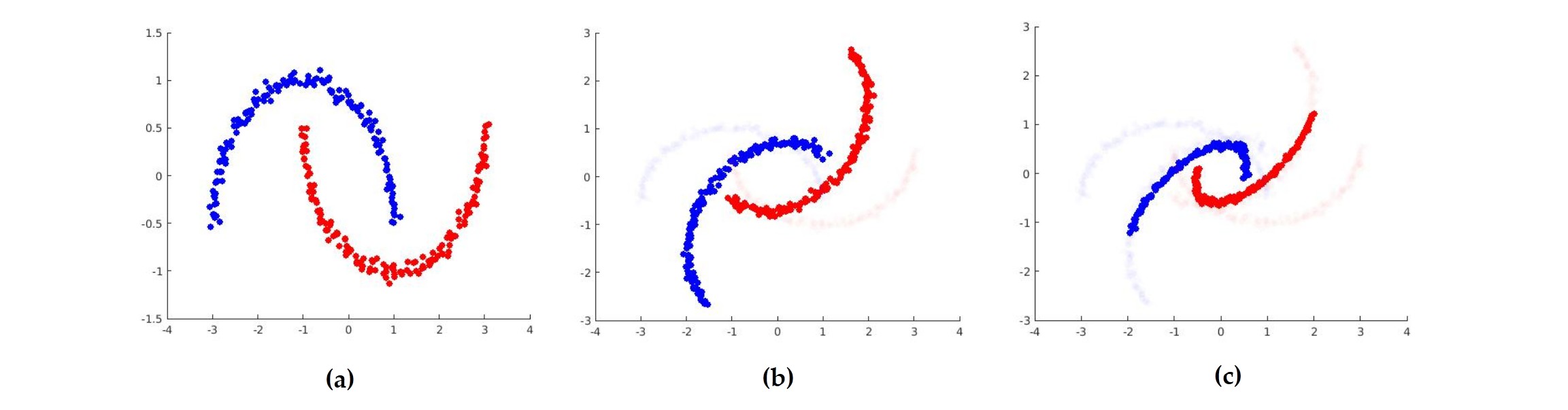
Figure 4: (a) Source-domain data. (b) Target-domain data consists of a 50-degree rotation of the source-domain data. (c) Transformed source-domain data is now aligned with the target-domain data.

5.1 Toy Dataset: Two interleaving moons

For the first experiment, we used the synthetic dataset of interleaving moons previously used in [10, 20]. The dataset consists of 2 domains. The source domain consists of 2 entangled moon’s data. Each moon is associated with each class. The target domain consists of applying a rotation to the source domain. This can be considered as a domain-adaptation problem with increasing rotation angle implying increasing difficulty of the domain-adaptation problem. Since the problem is low dimensional, it allowed us to visualize the effect of our domain-adaptation method appropriately. Figures 4(a) and 4(b) show an example of the source-domain data and the target-domain data respectively, and Fig. 4(c) shows the adapted source-domain data using the proposed approach. The results showed that the transformed source domain becomes close to the target domain.

For testing on this toy dataset, we used the same experimental protocol as in [10, 20]. We sampled 150 instances from the source domain and the same number of examples from the target domain. The test data was obtained by sampling 1000 examples from the target domain distribution. The classifier used is an SVM with a Gaussian kernel, whose parameters are set by 5-fold cross-validation. The experiments were conducted over 10 trials and the mean accuracy was reported. At this juncture, it is important to note that choosing the classifier for domain adaptation is important. For example, the two classes in the interleaving moon dataset are not linearly separable at all. So, a linear kernel SVM would not classify the moons accurately and it would result in poor performance in the target domain as well. That is why we need a Gaussian Kernel SVM. So, we have to make sure that we choose a classifier that works well with the source dataset in the first place.

Table 1: Accuracy results over 10 trials for the toy dataset domain-adaptation problem for varying degree of rotation between source and target domain

Angle (∘)	10	20	30	40	50	70	90
SVM-NA	100	89.6	76.0	68.8	60.0	23.6	17.2
DASVM	100	100	74.1	71.6	66.6	25.3	18.0
PBDA	100	90.6	89.7	77.5	59.8	37.4	31.3
OT-exact	100	97.2	93.5	89.1	79.4	61.6	49.3
OT-IT	100	99.3	94.6	89.8	87.9	60.2	49.2
OT-GL	100	100	100	98.7	81.4	62.2	49.2
OT-Laplace	100	100	99.6	93.8	79.9	59.8	47.6
Ours	100	100	96	87.4	83.9	78.4	72.2

We compared our results with the DA-SVM [7]- a domain-adaptive support vector machine approach, PBDA [20]- which is a PAC-Bayesian based domain adaptation method, and different versions of the optimal transport approach [10]. OT-exact is the basic optimal transport approach. OT-IT is the information theoretic version with entropy regularization. OT-GL and OT-Laplace has additional group and graph based regularization, respectively. From our results in Table 1, we see that for low rotation angles, the OT-GL-based method dominates and our proposed method yields satisfactory results. But for higher angles ($\geq$ 50 ^∘), our proposed method clearly dominates by a large margin. This is because we have taken into consideration second-order structural similarity information. For higher-rotation angles, the point-to-point sample distance is high. However, similar structures in the source and target domains can still correspond to each other. In other words, the adjacency matrices, which depend on relative distances between samples, can still be matched and do not depend on higher rotation angles between the source and target domains. That is why our proposed method out-performed other methods for large discrepancies between the source and target distributions.

We further provided the time comparison between the network simplex method (N-S) and MOSEK (M) for increasing number of samples of the toy dataset in Table 2. Results showed that the network simplex method is very fast compared to a general purpose linear programming solver like MOSEK.

Table 2: Time comparison (in seconds) of the two solvers for increasing sample size. The sample size is the number of samples per class per domain of the interleaving moon toy dataset. The target domain has a rotation of $50^{\circ}$ with the source domain. We use $N_{T}=1$. Implementation was in MATLAB in a workstation with Intel® Xeon(R) CPU E5-2630 v2 and 40 GB RAM. Results are reported over 10 trials.

$n$	25	50	75	100	125	150	175	200
M	62.1	83.1	103.4	128.5	387.7	680.1	1028.3	1577.6
N-S	1.5	4	6.9	10.1	16.9	23.5	31.2	41.3

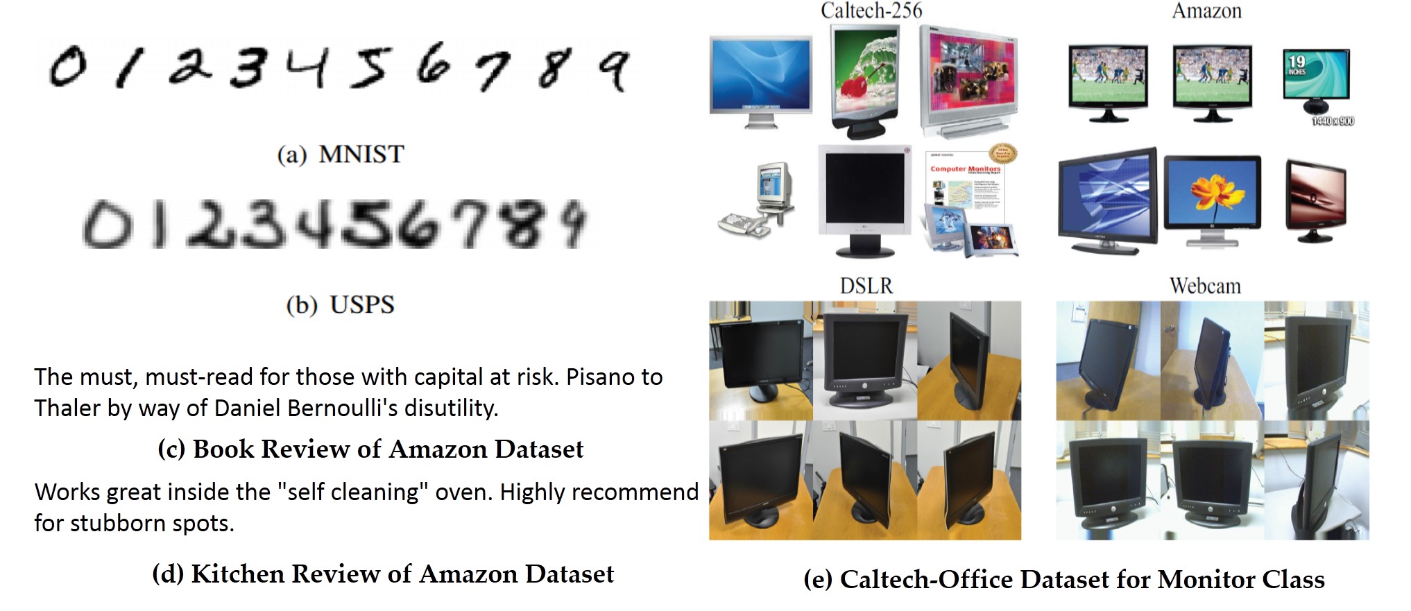
Figure 5: Instances of the real dataset used. At the top left, we see that USPS has the worse resolution compared to MNIST handwriting dataset. At the bottom left, we have instances of the Amazon review dataset. There is a shift in textual domain when reviewing for different products. On the right, we have the Caltech-Office dataset and we see that there are differences in illumination, quality, pose, presence/absence of background across different domains.

5.2 Real Dataset: Image Classification

We next evaluated the proposed method on image classification tasks. The image classification tasks that we considered were digit recognition and object recognition. The classifier used was 1-NN (Nearest Neighbor). 1-NN is used for experiments with images because it does not require cross-validating hyper-parameters and has been used in previous work as well [10, 23] The 1-NN classifier is trained on the transformed source-domain data and tested on the target-domain data. Instances of the image dataset are shown in Fig. 5 (a),(b) and (e). Generally, we cannot directly cross-validate our hyper-parameters $\lambda_{s}$ and $\lambda_{g}$ on the unlabelled target domain data making it impractical for real-world applications. However, for practical transfer learning purposes, a reverse validation (RV) technique[53] was developed for tuning the hyper-parameters. We have carried out experiments with a variant of the method to tune $\lambda_{s}$ and $\lambda_{g}$ for our UDA approach..

For a particular hyper-parameter configuration, we divide the source domain data into $K$ folds. We use one of the folds as the validation set. The remaining source data and the whole target data are used for domain adaptation. The classifier trained using the adapted source data is used to generate pseudo-labels for the target data. Another classifier is trained using the target domain data and its pseudo-labels. This classifier is then tested on the held-out source domain data after adaptation. The accuracy obtained is repeated and averaged over all the $K$ folds. This reverse-validation approach is repeated over all hyper-parameter configurations. The optimal hyper-parameter configuration is the one with the best average validation accuracy. Using the obtained optimal hyper-parameter configuration, we then carry out domain adaptation over all the source and target domain data and report the accuracy over the target domain dataset. We used $K=5$ folds for all the real-data experiments. Thus, we showed the results using this RV approach in addition to the best obtained results over the hyper-parameters. In majority of the cases in Tables 3,5,6 and 7 we would see that the result obtained using the reverse validation approach matches the best obtained results suggesting that the hyper-parameters can be automatically tuned successfully.

5.2.1 Digit Recognition

For the source and target domains, we used 2 datasets – USPS (U) and MNIST (M). These datasets have 10 classes in common (0-9). The dataset consists of randomly sampling 1800 and 2000 images from USPS and MNIST, respectively. The MNIST digits have $28\times 28$ resolution and the USPS $16\times 16$. The MNIST images were then resized to the same resolution as that of USPS. The grey levels were then normalized to obtain a common 256-dimensional feature space for both domains.

5.2.2 Object Recognition

For object recognition, we used the popular Caltech-Office dataset [23, 24, 41, 52, 10]. This domain-adaptation dataset consists of images from 4 different domains: Amazon (A) (E-commerce), Caltech-256 [27] (C) (a repository of images), Webcam (W) (webcam images), and DSLR (D) (images taken using DSLR camera). The differences between domains are due to the differences in quality, illumination, pose and also the presence and absence of backgrounds. The features used are the shallow SURF features [2] and deep-learning feature sets [13] – decaf6 and decaf7. The SURF descriptors represent each image as a 800-bin histogram. The histogram is first normalized to represent a probability and then reduced to standard z-scores. On the other hand, the deep-learning feature sets, decaf6 and decaf7, are extracted as the sparse activation of the neurons from the fully connected 6th and 7th layers of convolutional network trained on imageNet and fine tuned on our task. The features are 4096-dimensional.

For our experiments, we considered a random selection of 20 samples per class (with the exception of 8 samples per class for the DSLR domain) for the source domain. The target-domain data is split equally. One half of the target-domain data is used for domain adaptation and the other half is used for testing. This is in accordance with the protocol followed in [10]. The accuracy is reported on the test data over 10 trials of the experiment.

We compared our approach against (a) the no adaptation baseline (NA), which consists of using the original classifier without adaptation; (b) Geodesic Flow Kernel (GFK) [23]; (c) Transfer Subspace Learning (TSL) [42], which minimizes the Bregman divergence between low-dimensional embeddings of the source and target domains; (d) Joint Distribution Adaptation (JDA) [35], which jointly adapts both marginal and conditional distributions along with dimensionality reduction; (e) Optimal Transport [10] with the information-theoretic (OT-IT) and group-lasso version (OT-GL). Among all these methods, TSL and JDA are moment-matching methods while OT-IT, OT-GL and ours are sample-matching methods.

The best performing method for each domain-adaptation problem is highlighted in bold. From Table 3, we see that in almost all the cases, the OT-GL and our proposed method dominated over other methods, suggesting that sample-matching methods perform better than moment-matching methods. For the handwritten digit recognition tasks (U $\rightarrow$ M and M $\rightarrow$ U), our proposed method clearly out-performs GFK, TSL and JDA, but is slightly out-performed by OT-GL. This might be because the handwritten digit datasets U and M do not contain enough structurally similar regions to exploit the second-order similarity cost term. For the Office-Caltech dataset, the only time our proposed method was beaten by a moment-matching method was W $\rightarrow$ D, though by a slight amount. This is because W and D are closest pair of domains and using sample-based matching does not have outright advantage over moment-matching. The fact that W and D have the closest pair of domains is evident form the NA accuracy of 53.62, which is the best among NA accuracies of the Office-Caltech domain-adaptation tasks.

We have performed a runtime comparison in terms of the CPU time in seconds of our method with other methods and have shown the results in Table 4. The experiments performed are over the same dataset as used in Table 3. From Table 4, we see that local methods like OT-GL and our method generally take more time than moment-matching method like JDA. Our method takes more time compared with OT-GL because of time taken in constructing adjacency matrices for the second order cost term. Overall, the time taken for domain adaptation between USPS and MNIST datasets is more because they contain relatively larger number of samples, compared to the Office-Caltech dataset.

Table 3: Domain-adaptation results for digit recognition using USPS and MNIST datasets and object recognition with the Office-Caltech dataset using SURF features.

Tasks	NA	GFK	TSL	JDA	OT-GL	Ours	Ours (RV)
U $\rightarrow$ M	39.00	44.16	40.66	54.52	57.85	56.90	56.90
M $\rightarrow$ U	58.33	60.96	53.79	60.09	69.96	68.44	66.24
C $\rightarrow$ A	20.54	35.29	45.25	40.73	44.17	46.67	46.67
C $\rightarrow$ W	18.94	31.72	37.35	33.44	38.94	39.48	39.48
C $\rightarrow$ D	19.62	35.62	39.25	39.75	44.50	42.88	40.12
A $\rightarrow$ C	22.25	32.87	38.46	33.99	34.57	38.51	38.51
A $\rightarrow$ W	23.51	32.05	35.70	36.03	37.02	38.69	38.69
A $\rightarrow$ D	20.38	30.12	32.62	32.62	38.88	36.12	36.12
W $\rightarrow$ C	19.29	27.75	29.02	31.81	35.98	33.81	32.83
W $\rightarrow$ A	23.19	33.35	34.94	31.48	39.35	37.69	37.69
W $\rightarrow$ D	53.62	79.25	80.50	84.25	84.00	84.10	84.10
D $\rightarrow$ C	23.97	29.50	31.03	29.84	32.38	32.78	32.78
D $\rightarrow$ A	27.10	32.98	36.67	32.85	37.17	38.33	37.61
D $\rightarrow$ W	51.26	69.67	77.48	80.00	81.06	81.12	81.12

Table 4: CPU time (seconds) comparison of different domain adaptation algorithms.

Task	NA	GFK	TSL	JDA	OT-GL	Ours
U$\rightarrow$M	1.24	2.62	567.8	82.34	171.84	201.23
M$\rightarrow$U	1.13	2.43	522.37	81.13	168.23	196.15
C$\rightarrow$A	0.46	2.6	382.98	41.6	85.95	99.9
C$\rightarrow$W	0.24	1.45	157.52	37.89	78.73	101.1
C$\rightarrow$D	0.36	1.35	117.81	37.33	61.17	63.38
A$\rightarrow$C	0.54	2.69	462.12	40.11	105.87	126.18
A$\rightarrow$W	0.39	1.47	153.95	37.63	86.12	100.21
A$\rightarrow$D	0.42	1.31	115.87	36.82	69.29	82.1
W$\rightarrow$C	0.33	2.92	461.1	42.39	98.26	111.2
W$\rightarrow$A	0.61	2.52	388.23	41.64	94.38	101.45
W$\rightarrow$D	0.34	1.37	117.47	37.9	76.5	79.25
D$\rightarrow$C	0.45	2.36	364.13	39.75	106.21	118.12
D$\rightarrow$A	0.43	2.14	310.18	41.24	98.41	115.35
D$\rightarrow$W	0.24	1.05	93.73	34.62	76.23	88.69

Table 5: Domain-adaptation results for the Office-Caltech dataset using decaf6 features.

Task	NA	JDA	OT_IT	OT-GL	Ours	Ours(RV)
C$\rightarrow$A	79.25	88.04	88.69	92.08	91.92	89.91
C$\rightarrow$W	48.61	79.60	75.17	84.17	83.58	81.23
C$\rightarrow$D	62.75	84.12	83.38	87.25	87.50	87.50
A$\rightarrow$C	64.66	81.28	81.65	85.51	86.67	85.63
A$\rightarrow$W	51.39	80.33	78.94	83.05	81.39	81.39
A$\rightarrow$D	60.38	86.25	85.88	85.00	87.12	87.12
W$\rightarrow$C	58.17	81.97	74.80	81.45	82.13	81.64
W$\rightarrow$A	61.15	90.19	80.96	90.62	88.87	88.87
W$\rightarrow$D	97.50	98.88	95.62	96.25	98.95	98.95
D$\rightarrow$C	52.13	81.13	77.71	84.11	83.72	83.72
D$\rightarrow$A	60.71	91.31	87.15	92.31	92.65	92.65
D$\rightarrow$W	85.70	97.48	93.77	96.29	96.69	96.13

Table 6: Domain-adaptation results for the Office-Caltech dataset using decaf7 features.

Task	NA	JDA	OT-IT	OT-GL	Ours	Ours(RV)
C$\rightarrow$A	85.27	89.63	91.56	92.15	91.85	91.85
C$\rightarrow$W	65.23	79.80	82.19	83.84	85.36	85.36
C$\rightarrow$D	75.38	85.00	85.00	85.38	85.88	85.88
A$\rightarrow$C	72.80	82.59	84.22	87.16	86.67	85.39
A$\rightarrow$W	63.64	83.05	81.52	84.50	86.09	85.36
A$\rightarrow$D	75.25	85.50	86.62	85.25	87.37	87.37
W$\rightarrow$C	69.17	79.84	81.74	83.71	82.80	82.80
W$\rightarrow$A	72.96	90.94	88.31	91.98	90.15	89.31
W$\rightarrow$D	98.50	98.88	98.38	91.38	99.00	99.00
D$\rightarrow$C	65.23	81.21	82.02	84.93	82.20	82.20
D$\rightarrow$A	75.46	91.92	92.15	92.92	92.60	92.15
D$\rightarrow$W	92.25	97.02	96.62	94.17	97.10	97.10

We have also reported the results of Office-Caltech dataset using decaf6 and decaf7 features in Tables 5 and 6, respectively. The baseline performance of the deep-learning features are better than SURF features because they are more robust and contain higher-level representations. Expectedly, the decaf7 features have better baseline performance than decaf6 features. However, DA methods can further increase performance over the robust deep features. In Tables 5 and 6, we see that our proposed method dominates over JDA and OT-IT but is in close competition with OT-GL. We also noted that using decaf7 instead of decaf6 creates only a small incremental improvement in performance because most of the adaptation has already been performed by our proposed domain-adaptation method. As seen in Fig. 6, the source-domain samples are transformed to be near the target-domain samples using our proposed method. Therefore, we expect a classifier trained on the transformed source samples to perform better on the target-domain data.

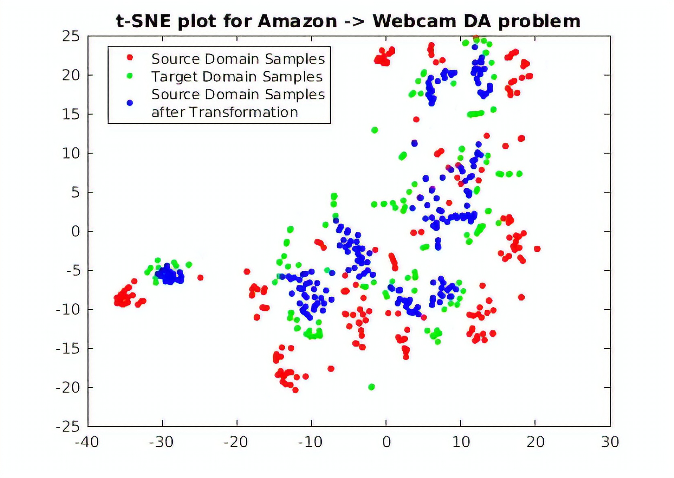
Figure 6: t-SNE [37] visualization of a single trial of Amazon to Webcam DA problem using decaf6 features.

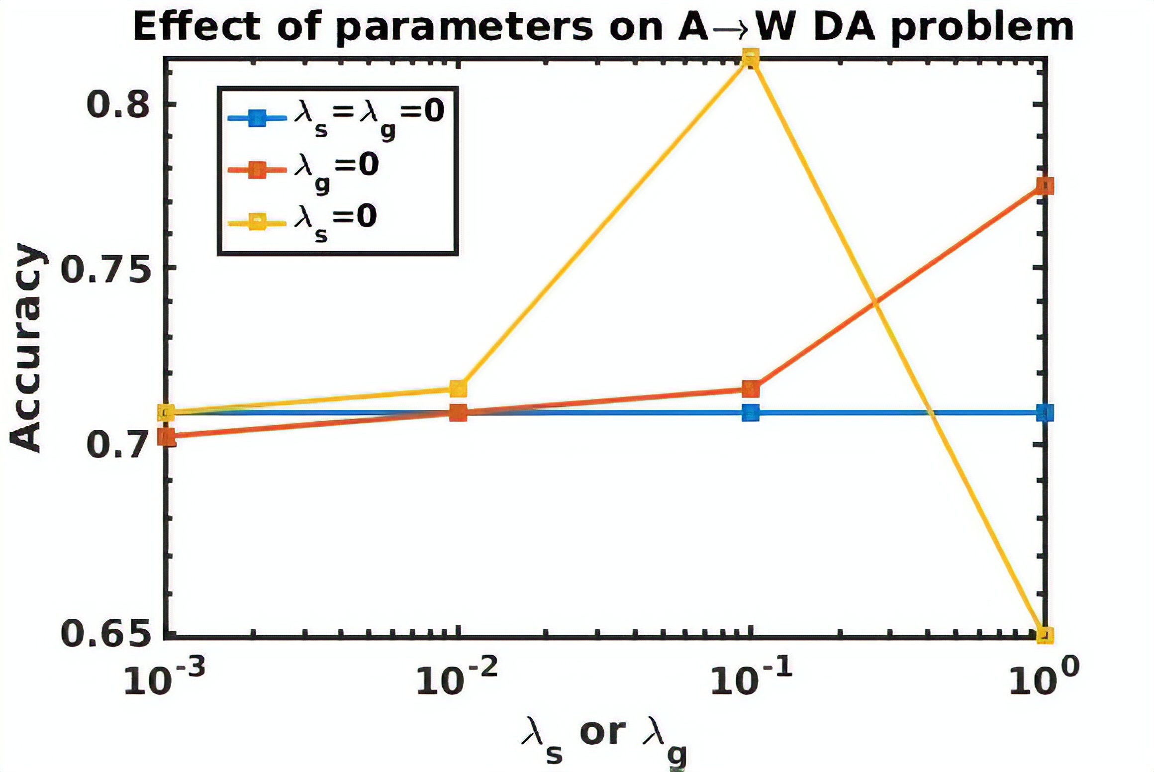
Figure 7: Effect of varying regularization parameters $\lambda_{s}$ and $\lambda_{g}$ on the accuracy of Amazon (source domain) to Webcam (target domain) visual domain-adaptation problem for fixed $N_{T}=1$.

We have also studied the effects of varying the regularization parameters on domain-adaptation performance. In Fig. 7, the blue line shows the accuracy when both $\lambda_{s}=\lambda_{g}=0$. When $\lambda_{s}=0$, best performance is obtained for $\lambda_{g}=0.1$. When $\lambda_{g}=0$, best performance is obtained for $\lambda_{g}=1$. For $\lambda_{s},\lambda_{g}>1$, performance degrades (not shown) because we have put excess weight on the regularization terms of second-order structural similarity and group-lasso than on the first-order point-wise similarity cost term. Thus, the presence of second-order and regularization term, weighted in the right amount is justified as it improves performance over when only the first-order term is present. We have also studied the effect of group-lasso regularization parameter ($\lambda_{g}$) on the quality of the correspondence matrix $\mathbf{C}$ obtained for a domain-adaptation task. Visually the second plot from the left in Fig. 8 appears to discriminate the 10 classes best. Accordingly, this parameter configuration ($\lambda_{s}=0,\lambda_{g}=0.1,N_{T}=1$) realizes the best performance as shown in the previous Fig. 7.

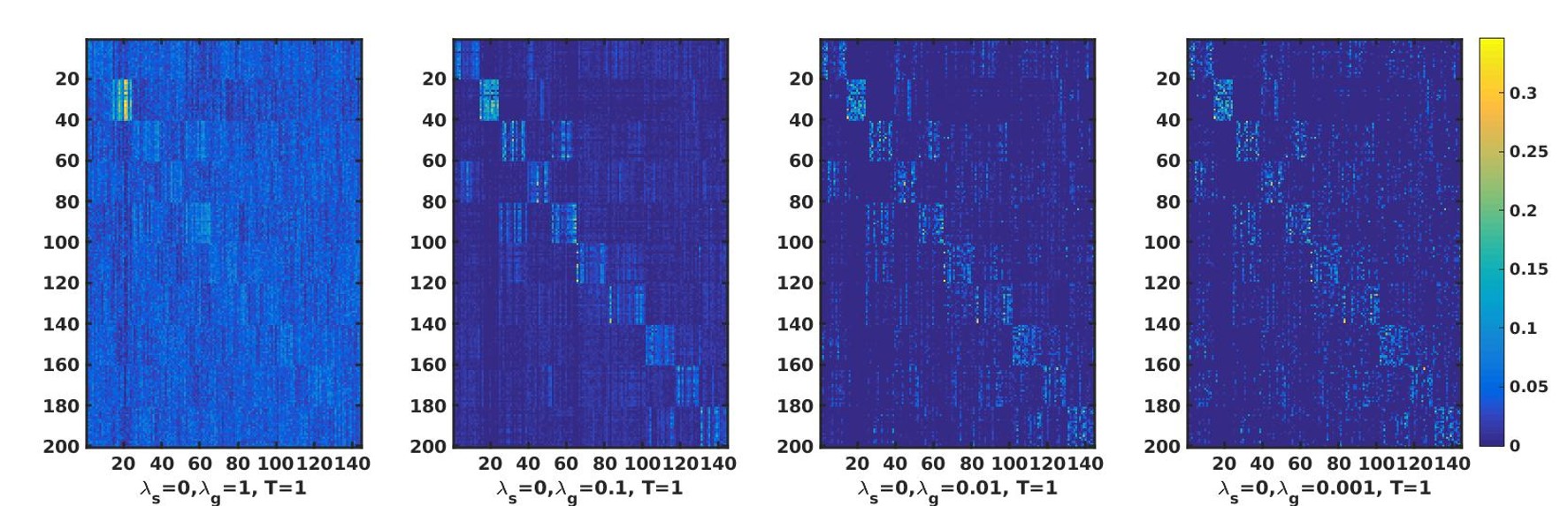
Figure 8: The optimal correspondence matrix ${\bf C}$ for 4 different parameter settings visualized as a colormap, with $\lambda_{s}=0,N_{T}=1$. The task involved was the Amazon to Webcam domain adaptation.

5.3 Real Dataset: Sentiment Classification

We have also evaluated our proposed method on sentiment classification using the standard Amazon review dataset [4]. This dataset contains Amazon reviews on 4 domains: Kitchen items (K), DVD (D), Books (B) and Electronics (E). Instances of the dataset are shown in Fig. 5 (c),(d). The dimensionality of the bag-of-word features was reduced by keeping the top 400 features having maximum mutual information with class labels. This pre-processing was also carried out in [44, 22] without losing performance. For each domain, we used 1000 positive and 1000 negative reviews. For each domain-adaptation task, we used 1600 samples (800 positive and 800 negative) from each domain as the training dataset. The remaining 400 samples (200 positive and 200 negative) were used for testing. The classifier used is a 1-NN classifier since it is parameter free. The mean-accuracy was reported over 10 random training/test splits.

We compared our proposed approach to a recently proposed unsupervised domain-adaptation approach known as Correlation Alignment (CORAL) [44]. CORAL is a simple and efficient approach that aligns the input feature distributions of the source and target domains by exploring their second-order statistics. Firstly, it computes the covariance statistics in each domain and then applies whitening and re-coloring linear transformation to the source features. Results in Table 7 showed that our proposed method outperforms CORAL in all the domain-adaptation tasks. Our proposed method has better performance because CORAL matches covariances while our method matches samples explicitly through point-wise and pair-wise matching. Moreover, CORAL does not use source-domain label information. Our method uses source-domain label information through the group-lasso regularization. However, CORAL is quite fast in transforming the source samples compared to our method. For a single trial, CORAL took about a second while our proposed method took about a few minutes.

Table 7: Accuracy results of unsupervised domain-adaptation tasks for the Amazon reviews dataset.

Tasks	K$\rightarrow$D	D$\rightarrow$B	B$\rightarrow$E	E$\rightarrow$K	K$\rightarrow$B	D$\rightarrow$E
NA	58.6	63.4	58.5	66.5	59.3	57.9
CORAL	59.9	66.5	59.5	67.5	59.2	59.5
Ours	63.5	69.5	62.0	69.5	64.5	61.2
Ours (RV)	60.9	69.5	62.0	69.5	64.5	59.0

6 Limitations

In this paper, we have assumed that the dimensionality of the source and target feature space is the same. Our approach cannot be directly used in cases when the dimensionality of the features are not the same. However, we can think of two ways in which this problem can be solved in conjunction with our approach. Firstly, we can add a preprocessing step where source and target domain is mapped to a latent space of the same dimensionality. Secondly, we can think of modifying the first-order matching term from $||{\bf C}{\bf X}^{t}-{\bf X}^{s}||^{2}_{\mathcal{F}}$ to $||{\bf C}{\bf X}^{t}-{\bf X}^{s}{\bf W}||^{2}_{\mathcal{F}}$. ${\bf W}$ belongs to $\mathbb{R}^{d\times d^{\prime}}$ where ${\bf W}$ maps from the source feature space $\mathbb{R}^{d}$ to the target feature space $\mathbb{R}^{d^{\prime}}$. But it would require properly regularizing ${\bf W}$.

Another question regarding our approach is whether our method is applicable to structured data. Structured data is stored in the form of databases or tables. These kind of data might contain numerical, categorical or date-time variables. The main problem in using structured data for our domain adaptation method is the presence of categorical variables. The presence of these discrete attributes would make the problem discontinuous and would not allow optimization to converge. However, we can use entity embedding [28], a recently developed method to map these categorical variables to an Euclidean Space. We can then use the embeddings of the categorical data as features for domain adaptation. However, we are yet to have standard domain adaptation datasets for structured data to test upon.

7 Conclusions

In this paper, we have described a correspondence-mapping method for unsupervised domain adaptation, which matched samples in the source domain with the samples in the target domain. Our proposed method is inspired from image registration, which alternately finds correspondences between samples and mapping between the corresponding samples. We proposed a convex-optimization-based approach to find the correspondence that consists of three cost terms: one for point-to-point similarity (first order), one for local structural similarity (second order), and another for class-based regularization. We have averted memory-efficiency problems of our optimization procedure by using the conditional gradient approach. We further averted the time-efficiency problem by solving the linear programming subproblems in conditional gradient method using a network simplex method of a min-cost flow problem, rather than a general purpose linear programming (LP) solver. An experiment on time-efficiency suggests that the network simplex method out-performs the general purpose LP solver by a large amount. Classification results on datasets of the textual and visual domain suggested that our proposed method outperformed other moment-matching methods and was comparable to previous sample-matching methods.

We believe that we can further improve our proposed method in terms of time and accuracy. Till now we have taken all the data-samples in the optimization procedure. We could efficiently search for “important” samples or exemplars that are a small fraction of all the data-samples. Consequently, the number of variables to optimize would be less and the optimization will be faster. As a result, the total time of finding the number of exemplars and the domain adaptation optimization procedure will be less. Also our method is a non-deep-learning method that directly works on features. We feel that extension of our method to deep architectures in terms of jointly learning a representation and the correspondences and mapping would improve performance in accuracy.

Appendix

Proof of convexity of optimization objective function

Let’s prove the convexity of each cost term in Eq. (2).

1. The first-order similarity term in the objective function is of the form $\|{\bf A}\|_{F}^{2}$, where ${\bf A}=\mathbf{CX}^{t}-{\bf X}^{s}$ is a matrix that linearly depends on ${\bf C}$. Here ${\bf A}\mapsto\|{\bf A}\|_{F}$ is a convex function due to the properties of norm. This convex function is composed with the function $x\mapsto x^{2}$, which is increasing and convex on the positive domain $[0,\infty)$. Thus, ${\bf A}\mapsto\|{\bf A}\|_{F}^{2}$ is the composition of a convex function with a convex increasing function, which makes it convex as well.

2. The argument for proving the convexity of second-order similarity term is similar to that of proving convexity of first-order similarity term except that ${\bf A}=\mathbf{CD}^{t}-{\bf D}^{s}{\bf C}$, which is linearly dependent on ${\bf C}$.

3. Proving the convexity of group-lasso regularization is easier. The group-lasso regularization term is a summation of $\ell_{2}$ norm terms. Now the set ${\bf C}$ is a convex set because it follows positivity and affine equality constraints [6]. So a subset of variables of ${\bf C}$ will also form a convex set. $\ell_{2}$ norm on any arbitrary such convex subset will produce a convex function. Summation of convex functions will yield a convex function and therefore the group-lasso regularization is convex.

Derivation of Gradients of the objective function

$$f_{1} =||{\bf C}{\bf X}^{t}-{\bf X}^{s}||^{2}_{\mathcal{F}}=\text{Tr}(({\bf C}{\bf X}^{t}-{\bf X}^{s})^{T}({\bf C}{\bf X}^{t}-{\bf X}^{s}))$$

$$=\text{Tr}(({\bf X}^{t})^{T}{\bf C}^{T}{\bf C}{\bf X}^{t}-({\bf X}^{t})^{T}{\bf C}^{T}{\bf X}^{s}-({\bf X}^{s})^{T}{\bf C}{\bf X}^{t}+({\bf X}^{s})^{T}{\bf X}^{s}),$$

and its gradient is

$$\nabla_{\mathbf{C}}f_{1} =\frac{\partial\text{{Tr}}(({\bf X}^{t})^{T}{\bf C}^{T}{\bf C}{\bf X}^{t})}{\partial{\bf C}}-\frac{\partial\text{Tr}(({\bf X}^{t})^{T}{\bf C}^{T}{\bf X}^{s})}{\partial{\bf C}}-\frac{\partial\text{Tr}(({\bf X}^{s})^{T}{\bf C}{\bf X}^{t})}{\partial{\bf C}}$$

$$=2{\bf C}{\bf X}^{t}({\bf X}^{t})^{T}-{\bf X}^{s}({\bf X}^{t})^{T}-{\bf X}^{s}({\bf X}^{t})^{T}=2({\bf C}{\bf X}^{t}-{\bf X}^{s})({\bf X}^{t})^{T}.$$

Let $r=\frac{n_{t}}{n_{s}}$, then

$$f_{2} =||{\bf C}{\bf D}^{t}-r{\bf D}^{s}{\bf C}||^{2}_{\mathcal{F}}=\text{Tr}(({\bf C}{\bf D}^{t}-r{\bf D}^{s}{\bf C})^{T}({\bf C}{\bf D}^{t}-r{\bf D}^{s}{\bf C}))$$

$$=\text{Tr}(({\bf D}^{t})^{T}{\bf C}^{T}{\bf C}{\bf D}^{t}-r({\bf D}^{t})^{T}{\bf C}^{T}{\bf D}^{s}{\bf C}-r{\bf C}^{T}({\bf D}^{s})^{T}{\bf C}{\bf D}^{t}+r^{2}{\bf C}^{T}({\bf D}^{s})^{T}{\bf D}^{s}{\bf C}),$$

and its gradient can be obtained as

$$\nabla_{\mathbf{C}}f_{2} =\frac{\partial\text{Tr}(({\bf D}^{t})^{T}{\bf C}^{T}{\bf C}{\bf D}^{t})}{\partial{\bf C}}-\frac{\partial\text{Tr}(r({\bf D}^{t})^{T}{\bf C}^{T}{\bf D}^{s}{\bf C})}{\partial{\bf C}}$$

$$\quad-\frac{\partial\text{Tr}(r{\bf C}^{T}({\bf D}^{s})^{T}{\bf C}{\bf D}^{t})}{\partial{\bf C}}+\frac{\partial\text{Tr}(r^{2}{\bf C}^{T}({\bf D}^{s})^{T}{\bf D}^{s}{\bf C})}{\partial{\bf C}}$$

$$=2{\bf C}{\bf D}^{t}({\bf D}^{t})^{T}-2r{\bf D}^{s}{\bf C}({\bf D}^{t})^{T}-2r({\bf D}^{s})^{T}{\bf C}{\bf D}^{t}+2r^{2}({\bf D}^{s})^{T}{\bf D}^{s}{\bf C}.$$

$\nabla_{\mathbf{C}}f_{3}$ can be found by carrying out the partial derivative $\frac{\partial f_{3}}{\partial[{\bf C}]_{ij}}$ with respect to each element $[{\bf C}]_{ij}$ of the correspondence matrix.

$$\frac{\partial f_{3}}{\partial[{\bf C}]_{ij}}=\frac{\partial(\sum_{j}\sum_{c}||[{\bf C}]_{\mathcal{I}_{c}j}||_{2})}{\partial[{\bf C}]_{ij}}=\frac{\partial(||[{\bf C}]_{\mathcal{I}_{c(i)}j}||_{2})}{\partial[{\bf C}]_{ij}}.$$

Here, $c(i)$ is the class corresponding to the $i^{th}$ sample in the source domain. The other summation terms are omitted because they do not depend on $[{\bf C}]_{ij}$. Using the property that partial derivative of an $\ell_{2}$-norm with respect to an element; that is, $\frac{\partial(||{\bf x}||_{2})}{\partial x_{i}}=\frac{x_{i}}{||{\bf x}||_{2}}$ , we have

$$\frac{\partial(||[{\bf C}]_{\mathcal{I}_{c}j}||_{2})}{\partial[{\bf C}]_{ij}}=\frac{[{\bf C}]_{ij}}{||[{\bf C}]_{\mathcal{I}_{c}(i)j}||_{2}}.$$

However, the group-lasso regularization term $f_{3}$ is not differentiable if there exists a class $c$ and an index $j$ (corresponding to the $j^{\rm th}$ sample of the target domain) such that $||[{\bf C}]_{\mathcal{I}_{c}j}||_{2}=0$. In such a case, we set the partial derivative of the corresponding terms to $0$. Thus, the gradient of the group-lasso term is found as follows:

$$\frac{\partial f_{3}}{\partial[{\bf C}]_{ij}}=\begin{cases}\frac{[{\bf C}]_{ij}}{||[{\bf C}]_{\mathcal{I}_{c}(i)j}||_{2}}~{},&\text{if }||[{\bf C}]_{\mathcal{I}_{c}(i)j}||_{2}\neq 0;\\ 0~{},&\text{otherwise;}\end{cases}$$

where $c(i)$ is the class corresponding to the $i^{th}$ sample in the source domain.

References

- Andersen [2013] Andersen, E. D., 2013. Complexity of solving conic quadratic problems. http://erlingdandersen.blogspot.com/2013/11/complexity-of-solving-conic-quadratic.html, accessed: 2010-09-30.
- Bay et al. [2006] Bay, H., Tuytelaars, T., Van Gool, L., 2006. Surf: Speeded up robust features. In: European Conf. Computer Vision. pp. 404–417.
- Besl and McKay [1992] Besl, P. J., McKay, N. D., 1992. Method for registration of 3-d shapes. In: Proc. Intern. Society Optics Photonics. International Society for Optics and Photonics, pp. 586–606.
- Blitzer et al. [2007] Blitzer, J., Dredze, M., Pereira, F., 2007. Biographies, bollywood, boom-boxes and blenders: Domain adaptation for sentiment classification. In: Proc. Annual Meeting Association Computational Linguistics. pp. 440–447.
- Borgwardt et al. [2006] Borgwardt, K. M., Gretton, A., Rasch, M. J., Kriegel, H.-P., Schölkopf, B., Smola, A. J., 2006. Integrating structured biological data by kernel maximum mean discrepancy. Bioinformatics 22 (14), e49–e57.
- Boyd and Vandenberghe [2004] Boyd, S., Vandenberghe, L., 2004. Convex optimization. Cambridge university press.
- Bruzzone and Marconcini [2010] Bruzzone, L., Marconcini, M., 2010. Domain adaptation problems: A dasvm classification technique and a circular validation strategy. IEEE Trans. Pattern Anal. Mach. Intell. 32 (5), 770–787.
- Chen et al. [2012] Chen, M., Xu, Z., Weinberger, K., Sha, F., 2012. Marginalized denoising autoencoders for domain adaptation. arXiv preprint arXiv:1206.4683.
- Chui and Rangarajan [2003] Chui, H., Rangarajan, A., 2003. A new point matching algorithm for non-rigid registration. Computer Vision and Image Understanding 89 (2), 114–141.
- Courty et al. [2017] Courty, N., Flamary, R., Tuia, D., Rakotomamonjy, A., 2017. Optimal transport for domain adaptation. IEEE Trans. Pattern Anal. Mach. Intell. 39 (9), 1853–1865.
- Csurka [2017] Csurka, G., 2017. Domain adaptation for visual applications: A comprehensive survey. arXiv preprint arXiv:1702.05374.
- Daumé III [2009] Daumé III, H., 2009. Frustratingly easy domain adaptation. arXiv preprint arXiv:0907.1815.
- Donahue et al. [2014] Donahue, J., Jia, Y., Vinyals, O., Hoffman, J., Zhang, N., Tzeng, E., Darrell, T., 2014. Decaf: A deep convolutional activation feature for generic visual recognition. In: Intern. Conf. Machine Learning. pp. 647–655.
- Duan et al. [2009] Duan, L., Tsang, I. W., Xu, D., Maybank, S. J., 2009. Domain transfer svm for video concept detection. In: Proc. IEEE Conference on Computer Vision and Pattern Recognition (CVPR). pp. 1375–1381.
- Duchenne et al. [2011] Duchenne, O., Bach, F., Kweon, I.-S., Ponce, J., 2011. A tensor-based algorithm for high-order graph matching. IEEE Trans. Pattern Anal. Mach. Intell. 33 (12), 2383–2395.
- Farajidavar et al. [2014] Farajidavar, N., de Campos, T. E., Kittler, J., 2014. Adaptive transductive transfer machine. In: British Machine Vision Conference.
- Fernando et al. [2013] Fernando, B., Habrard, A., Sebban, M., Tuytelaars, T., 2013. Unsupervised visual domain adaptation using subspace alignment. In: Proc. IEEE Int. Conf. Computer Vision. pp. 2960–2967.
- Frank and Wolfe [1956] Frank, M., Wolfe, P., 1956. An algorithm for quadratic programming. Naval Research Logistics (NRL) 3 (1-2), 95–110.
- Ganin et al. [2016] Ganin, Y., Ustinova, E., Ajakan, H., Germain, P., Larochelle, H., Laviolette, F., Marchand, M., Lempitsky, V., 2016. Domain-adversarial training of neural networks. Journal of Machine Learning Research 17 (59), 1–35.
- Germain et al. [2013] Germain, P., Habrard, A., Laviolette, F., Morvant, E., 2013. A pac-bayesian approach for domain adaptation with specialization to linear classifiers. In: Intern. Conf. Machine Learning. pp. 738–746.
- Ghifary et al. [2015] Ghifary, M., Bastiaan Kleijn, W., Zhang, M., Balduzzi, D., 2015. Domain generalization for object recognition with multi-task autoencoders. In: Proc. IEEE Int. Conf. Computer Vision. pp. 2551–2559.
- Gong et al. [2013] Gong, B., Grauman, K., Sha, F., 2013. Connecting the dots with landmarks: Discriminatively learning domain-invariant features for unsupervised domain adaptation. In: Intern. Conf. Machine Learning. pp. 222–230.
- Gong et al. [2012] Gong, B., Shi, Y., Sha, F., Grauman, K., 2012. Geodesic flow kernel for unsupervised domain adaptation. In: Proc. IEEE Conference on Computer Vision and Pattern Recognition (CVPR). pp. 2066–2073.
- Gopalan et al. [2011] Gopalan, R., Li, R., Chellappa, R., 2011. Domain adaptation for object recognition: An unsupervised approach. In: Proc. IEEE Int. Conf. Computer Vision. pp. 999–1006.
- Gopalan et al. [2014] Gopalan, R., Li, R., Chellappa, R., 2014. Unsupervised adaptation across domain shifts by generating intermediate data representations. IEEE Trans. Pattern Anal. Mach. Intell. 36 (11), 2288–2302.
- Gretton et al. [2009] Gretton, A., Smola, A., Huang, J., Schmittfull, M., Borgwardt, K., Schölkopf, B., 2009. Covariate shift by kernel mean matching. Dataset Shift in Machine Learning 3 (4), 5.
- Griffin et al. [2007] Griffin, G., Holub, A., Perona, P., 2007. Caltech-256 object category dataset. Tech. Rep. 7694, California Institute of Technology.
- Guo and Berkhahn [2016] Guo, C., Berkhahn, F., 2016. Entity embeddings of categorical variables. arXiv preprint arXiv:1604.06737.
- Huang et al. [2007] Huang, J., Smola, A. J., Gretton, A., Borgwardt, K. M., Schölkopf, B., 2007. Correcting sample selection bias by unlabeled data. In: Advances in Neural Information Processing Systems. p. 601.
- Jaggi [2013] Jaggi, M., 2013. Revisiting frank-wolfe: Projection-free sparse convex optimization. In: Intern. Conf. Machine Learning. pp. 427–435.
- Jiang et al. [2008] Jiang, W., Zavesky, E., Chang, S.-F., Loui, A., 2008. Cross-domain learning methods for high-level visual concept classification. In: Proc. IEEE Int. Conf. Image Processing. pp. 161–164.
- Kanamori et al. [2009] Kanamori, T., Hido, S., Sugiyama, M., 2009. Efficient direct density ratio estimation for non-stationarity adaptation and outlier detection. In: Advances in Neural Information Processing Systems. pp. 809–816.
- Kelly [1991] Kelly, D. J., 1991. The minimum cost flow problem and the network simplex solution method. Ph.D. thesis.
- Long et al. [2015] Long, M., Cao, Y., Wang, J., Jordan, M. I., 2015. Learning transferable features with deep adaptation networks. In: Intern. Conf. Machine Learning. pp. 97–105.
- Long et al. [2013] Long, M., Wang, J., Ding, G., Sun, J., Yu, P. S., 2013. Transfer feature learning with joint distribution adaptation. In: Proc. IEEE Int. Conf. Computer Vision. pp. 2200–2207.
- Long et al. [2016] Long, M., Wang, J., Jordan, M. I., 2016. Deep transfer learning with joint adaptation networks. arXiv preprint arXiv:1605.06636.
- Maaten and Hinton [2008] Maaten, L. v. d., Hinton, G., 2008. Visualizing data using t-sne. Journal of Machine Learning Research 9 (Nov), 2579–2605.
- Mosek [2010] Mosek, A., 2010. The mosek optimization software. Online at http://www. mosek. com 54, 2–1.
- Pan et al. [2011] Pan, S. J., Tsang, I. W., Kwok, J. T., Yang, Q., 2011. Domain adaptation via transfer component analysis. IEEE Trans. Neural Networks 22 (2), 199–210.
- Pan and Yang [2010] Pan, S. J., Yang, Q., 2010. A survey on transfer learning. IEEE Trans. Knowledge Data Engg. 22 (10), 1345–1359.
- Saenko et al. [2010] Saenko, K., Kulis, B., Fritz, M., Darrell, T., 2010. Adapting visual category models to new domains. In: European Conf. Computer Vision. pp. 213–226.
- Si et al. [2010] Si, S., Tao, D., Geng, B., 2010. Bregman divergence-based regularization for transfer subspace learning. IEEE Trans. Knowledge Data Engg. 22 (7), 929–942.
- Sugiyama et al. [2008] Sugiyama, M., Nakajima, S., Kashima, H., Buenau, P. V., Kawanabe, M., 2008. Direct importance estimation with model selection and its application to covariate shift adaptation. In: Advances in Neural Information Processing Systems. pp. 1433–1440.
- Sun et al. [2016] Sun, B., Feng, J., Saenko, K., 2016. Return of frustratingly easy domain adaptation. In: Thirtieth AAAI Conference on Artificial Intelligence.
- Sun and Saenko [2016] Sun, B., Saenko, K., 2016. Deep coral: Correlation alignment for deep domain adaptation. In: European Conf. Computer Vision Workshops. pp. 443–450.
- Torralba and Efros [2011] Torralba, A., Efros, A. A., 2011. Unbiased look at dataset bias. In: Proc. IEEE Conference on Computer Vision and Pattern Recognition (CVPR). pp. 1521–1528.
- Tzeng et al. [2017] Tzeng, E., Hoffman, J., Saenko, K., Darrell, T., 2017. Adversarial discriminative domain adaptation. arXiv preprint arXiv:1702.05464.
- Tzeng et al. [2014] Tzeng, E., Hoffman, J., Zhang, N., Saenko, K., Darrell, T., 2014. Deep domain confusion: Maximizing for domain invariance. arXiv preprint arXiv:1412.3474.
- Weiss et al. [2016] Weiss, K., Khoshgoftaar, T. M., Wang, D., 2016. A survey of transfer learning. Journal of Big Data 3 (1), 1–40.
- Yang et al. [2007] Yang, J., Yan, R., Hauptmann, A. G., 2007. Cross-domain video concept detection using adaptive svms. In: Proc. ACM Int. Conf. on Multimedia. pp. 188–197.
- Zadrozny [2004] Zadrozny, B., 2004. Learning and evaluating classifiers under sample selection bias. In: Intern. Conf. Machine Learning. p. 114.
- Zheng et al. [2012] Zheng, J., Liu, M.-Y., Chellappa, R., Phillips, P. J., 2012. A grassmann manifold-based domain adaptation approach. In: Proc. IEEE Int. Conf. Pattern Recognition. pp. 2095–2099.
- Zhong et al. [2010] Zhong, E., Fan, W., Yang, Q., Verscheure, O., Ren, J., 2010. Cross validation framework to choose amongst models and datasets for transfer learning. In: Joint European Conference on Machine Learning and Knowledge Discovery in Databases. pp. 547–562.