Separable correlation and maximum likelihood

Abstract

We consider estimation of the covariance matrix of a multivariate normal distribution when the correlation matrix is separable in the sense that it factors as a Kronecker product of two smaller matrices. A computationally convenient coordinate descent-type algorithm is developed for maximum likelihood estimation. Simulations indicate our method often gives smaller estimation error than some common alternatives when correlation is separable, and that correctly sized tests for correlation separability can be obtained using a parametric bootstrap. Using dissolved oxygen data from the Upper Mississippi River, we illustrate how our model can lead to interesting scientific findings that may be missed when using competing models.

1 Introduction

Many statistical applications require the estimation of a covariance matrix $\mathrm{cov}(Y_{i})=\Sigma\in\mathbb{S}^{q}_{++}$, the set of $q\times q$ symmetric, positive definite matrices, for some $\mathbb{R}^{q}$-valued random vectors $Y_{i}$ $(i=1,\dots,n$). When the number of observations is small, meaning $n<q$ if there are no other parameters to be estimated, and the vectors are multivariate normal, a maximum likelihood estimate of $\Sigma$ does not exist. Two common ways to estimate $\Sigma$ in such settings are shrinkage estimators, see e.g. Fan et al., (2016), and more parsimonious parameterizations, which may also result from application specific considerations. In the spatio-temporal literature it is sometimes assumed that the covariance is separable (Cressie and Wikle,, 2011, section 6.1.3) in the sense that $\Sigma$ factors as a Kronecker product of two smaller covariance matrices. In this article we consider estimation of $\Sigma$ when the corresponding correlation matrix $R=\mathrm{cor}(Y_{i})$ ($i=1,\dots,n$) is separable, but $\Sigma$ need not be. Mathematically, $R=U\otimes V$ for some $U\in\mathbb{C}^{c}_{++}$ and $V\in\mathbb{C}^{r}_{++}$, where $\mathbb{C}^{k}_{++}$ is the set of definite $k\times k$ correlation matrices, $\otimes$ denotes the Kronecker product, and $rc=q$. As we shall see, this is a weaker assumption than covariance separability that still, often substantially, reduces the number of parameters compared to an unrestricted covariance matrix.

Correlation separability has a natural interpretation for two-dimensional, or matrix-valued, data. If $\mathbf{Y}_{i}\in\mathbb{R}^{r\times c}$ $(i=1,\dots,n)$ is a random matrix such that $\mathrm{vec}(\mathbf{Y}_{i})=Y_{i}$, where $\mathrm{vec}(\cdot)$ is the vectorization operator stacking the columns of its matrix argument, then every row of $\mathbf{Y}_{i}$ has the same correlation matrix $U$, and every column of $\mathbf{Y}_{i}$ has the same correlation matrix $V$. In our example with spatio-temporal data, rows of $\mathbf{Y}_{i}$ correspond to different sampling locations, or areas, and the columns to different points in time. Then separability of $R$ says that the temporal autocorrelation function for observations from any one location $i$ is the same as that for observations from any other location $j$ ($i=1,\dots,r$, $j=1,\dots,r$). Similarly, the spatial autocorrelation function is the same for all time points.

To the best of our knowledge, previous research on correlation separability has been concerned with models that also impose other restrictions on $\Sigma$, which we do not. For example, both Matsuda and Yajima, (2004) and Ren et al., (2013) consider models with separable correlation, but make additional assumptions that, taken together with correlation separability, implies covariance separability. A considerable amount of research has been done on models with separable covariance, which when $Y_{i}$ is multivariate normal is equivalent to assuming that $\mathbf{Y}_{i}$ has a matrix normal distribution. For example, Dutilleul and Pinel-Alloul, (1996) suggest the matrix normal distribution for analyzing spatio-temporal data, Soloveychik and Trushin, (2016) give theoretical results for the existence and uniqueness of maximum likelihood estimates of $U$ and $V$, and Ding and Cook, (2017) develop envelope methods for regressions with matrix-valued responses.

2 The Separable Correlation Model

We assume that $y_{1},\dots,y_{n}$ are realizations of $n$ independent, multivariate normal $q$-vectors $Y_{1},\dots,Y_{n}$ with means $E(Y_{i})=\beta^{T}x_{i}$ for some non-stochastic predictors $x_{i}\in\mathbb{R}^{p}$ ($i=1,\dots,n$) and parameter matrix $\beta\in\mathbb{R}^{p\times q}$. Since the focus of this article is the structure in $\Sigma$, we often take $x_{i}=1$ ($i=1,\dots,n$) for simplicity, but it’s useful to allow for predictors in many applications, including our data example. Our model is thus a multivariate linear regression model with separable correlation matrix, which we for short call the separable correlation model. We refer the reader to, for example, Rencher and Christensen, (2012, chapter 10) for a discussion of the classical multivariate linear regression model with focus on $\beta$.

It’s easy to show that any $\Sigma\in\mathbb{S}^{q}_{++}$ can be decomposed as $\Sigma=WRW$, where $W$ is a diagonal matrix with diagonal entries equal to the positive square roots of the diagonal entries of $\Sigma$, i.e. the standard deviations of the elements in $Y_{i}$ ($i=1,\dots,n$), and $R=\mathrm{cor}(Y_{i})$ ($i=1,\dots,n$). We call diagonal matrices with positive entries, like $W$, standard deviation matrices. From writing $\Sigma$ in terms of $W$ and $R$ it follows that the assumption of separable correlation can also be written $\Sigma=W(U\otimes V)W$. The negative log-likelihood for $n$ observations in our model is thus, up to scaling and additive constants,

$$g(\beta,U,V,W) =\log|W(U\otimes V)W|+\mathrm{tr}\left(S^{\star}[W(U\otimes V)W]^{-1}\right),$$ (1)

where $S^{\star}=S^{\star}(\beta)=\sum_{i=1}^{n}(y_{i}-\beta^{T}x_{i})(y_{i}-\beta^{T}x_{i})^{T}/n$ and $|\cdot|$ denotes the determinant of its matrix argument.

The multivariate linear regression model with separable covariance, which we call the separable covariance model, or the matrix normal model when $x_{i}=1$ ($i=1,\dots,n$), is a special case of our model. Indeed, if the standard deviation matrix is also separable so that $W=W_{U}\otimes W_{V}$ for some $r\times r$ and $c\times c$ standard deviation matrices $W_{U}$ and $W_{r}$, then $W(U\otimes V)W=(W_{U}UW_{U})\otimes(W_{V}VW_{V})=\tilde{U}\otimes\tilde{V}$, where $\tilde{U}$ and $\tilde{V}$ are covariance matrices defined by the last equality. Given the similarities, we view the separable covariance model as the closest competitor to our model and, hence, use it for comparisons throughout. The difference between the models is that in the the separable covariance model the variances must satisfy $\mathrm{var}(Y_{i,j,k})=W_{V,j,j}^{2}W_{U,k,k}^{2}$; in our model there are no parametric restrictions on the variance structure. Here, $Y_{i,j,k}$ is the element in row $j$ and column $k$ of $\mathbf{Y}_{i}$, $W_{U,k,k}$ is the $k$th diagonal entry of $W_{U}$, and similarly for $W_{V,j,j}$. When the rows of $\mathbf{Y}_{i}$ index sampling locations and the columns index time points, this restriction rules out the possibility that for one sampling location the variability of measurements is largest in time period one, whereas for another location it is largest in time period two, for example. In our data example we shall see that this may be too restrictive. The flexibility in variance structure offered by the separable correlation model requires $rc-r-c+1$ parameters more than what is needed in the separable covariance model. The difference results from the fact that there are $rc$ standard deviation parameters in the separable correlation model, namely the diagonal entries of $W$. In the separable covariance model there are $r+c-1$ variance parameters, namely the diagonal entries of $U$ and $V$, minus one due to an identifiability constraint explained below. The correlations structure is the same for both models and hence requires the same number of parameters. While the difference in total parameter counts may be substantial for some settings, it is notable that, as $(r,c)\to(\infty,\infty)$, the total number of covariance parameters is of the order $r^{2}+c^{2}$ for both models while it is of the order $(rc)^{2}$ for an unstructured covariance matrix.

When $\Sigma=U\otimes V$ for some covariance matrices $U$ and $V$, then for any constant $c>0$, the matrices $cU$ and $V/c$ are also covariance matrices, and $(cU)\otimes(V/c)=U\otimes V$. That is, $U$ and $V$ are not identified unless additional restrictions are imposed. One possible restriction that ensures identifiability is that $U_{1,1}=1$, which leads to the difference in parameter counts stated above. Proposition 1 shows that no additional restrictions are needed to identify the parameters in the the separable correlation model. All proofs are in the supplemental material.

Proposition 1

If $g(\beta,U,V,W)=g(\beta^{\prime},U^{\prime},V^{\prime},W^{\prime})$ for Lebesgue-almost every $y_{1},\dots,y_{n}$ and $X=(x_{1},\dots,x_{n})^{T}$ has full column rank, then $(\beta,U,V,W)=(\beta^{\prime},U^{\prime},V^{\prime},W^{\prime})$.

3 Maximum Likelihood

To obtain maximum likelihood estimates, $g$ is minimized jointly in $(\beta,U,V,W)$. The coefficient $\beta$ can be profiled out of the optimization problem before considering $U,V,W$ in more detail. Differentiating $g$ with respect to $\beta$, and twice with respect to $\mathrm{vec}(\beta)$, one gets

$$\nabla_{\beta}g=-n^{-1}\sum_{i=1}^{n}[x_{i}y_{i}^{T}-x_{i}x_{i}^{T}\beta]\Sigma^{-1},\quad\nabla^{2}_{\mathrm{vec}(\beta)}g=\Sigma^{-1}\otimes\sum_{i=1}^{n}x_{i}x_{i}^{T}/n.$$

Thus, assuming $\sum_{i=1}^{n}x_{i}x_{i}^{T}=X^{T}X$ is invertible, which we do throughout, $g$ is strictly convex in $\mathrm{vec}(\beta)$, and the unique partial minimizer in $\beta$ is the least squares estimator $\hat{\beta}=(X^{T}X)^{-1}X^{T}Y$, where $Y=(Y_{1},\dots,Y_{n})^{T}\in\mathbb{R}^{n\times q}$. We shall use hats to denote maximum likelihood estimates, and subscripts $cor$ and $cov$ to indicate whether they are from the separable correlation or covariance model, respectively. Since $\hat{\beta}$ is the same regardless of $\Sigma$, we omit the subscript. The rest of this article is focused on minimizing the objective function $g_{1}$ defined by $g_{1}(U,V,W)=g(\hat{\beta},U,V,W)$ and studying the properties of those minimizers, i.e. the maximum likelihood estimates of the covariance parameters.

The minimizers of $g_{1}$ cannot be expressed in closed form. In the separable covariance model where $U$ and $V$ are covariance matrices, $\hat{\Sigma}_{\mathrm{cov}}$ can be found using the so called flip-flop algorithm of Dutilleul, (1999), given that $n$ is large enough in comparison to $r$ and $c$ (Soloveychik and Trushin,, 2016). The flip-flop algorithm is essentially a coordinate descent algorithm where the iterates are rescaled for identifiability reasons at every iteration. The algorithm we develop here, Algorithm 1, builds on similar ideas. More specifically, the idea is to update, or iteratively optimize, $g_{1}$ coordinate by coordinate over a strictly larger space than the parameter space, and then use a type of rescaling to force the iterates to lie in the original parameter space. We next walk through the execution of this idea more formally.

When deriving updates for $W$ we consider the diagonal entries individually and write, with some overloading of notation, $g_{1}(U,V,w_{1},\dots,w_{q})=g_{1}(U,V,\mathrm{diag}(w_{1},\dots,w_{q}))$, where $\mathrm{diag}(w_{1},\dots,w_{q})$ denotes the $q\times q$ diagonal matrix with diagonal entries $w_{1},\dots,w_{q}$. Treating the diagonal elements of $W$ separately, the function $g_{1}$ is formally defined on $\mathsf{X}=\mathbb{C}^{c}_{++}\times\mathbb{C}^{r}_{++}\times(0,\infty)\times\dots\times(0,\infty)$. Some steps in the derivation of the algorithm we propose for minimizing $g_{1}$ require we extend it to the space $\mathsf{Y}=\mathbb{S}^{c}_{++}\times\mathbb{S}^{r}_{++}\times(0,\infty)\times\dots\times(0,\infty)$. That is, in some steps we allow $U$ and $V$ to be general covariance matrices. For simplicity, we still denote the extension by $g_{1}$ and write $g_{1}(\mathsf{y})=g_{1}(U,V,w_{1},\dots,w_{q})$, for all $\mathsf{y}=(U,V,w_{1},\dots,w_{q})\in\mathsf{Y}$. We also write $\Sigma=\Sigma(\mathsf{y})=W(U\otimes V)W$ to indicate that $\Sigma$ can be viewed as a function of $\mathsf{y}\in\mathsf{Y}$. Extending $g_{1}$ to $\mathsf{Y}$ makes the parameters, or optimization variables, $U$, $V$, $w_{1}$, …, $w_{q}$, unidentifiable in the sense that we can find two, in fact infinitely many, $\mathsf{y},\mathsf{y}^{\prime}\in\mathsf{Y}$ such that $\Sigma(\mathsf{y})=\Sigma(\mathsf{y}^{\prime})$, and hence $g_{1}(\mathsf{y})=g_{1}(\mathsf{y}^{\prime})$. However, Proposition 2 shows that we can identify each point in $\mathsf{Y}$ with one in $\mathsf{X}$, where each point corresponds to exactly one $\Sigma$, i.e. the parameters are identified.

Proposition 2

For every point $\mathsf{y}\in\mathsf{Y}$, there is a unique point $\mathsf{x}\in\mathsf{X}$ such that $\Sigma(\mathsf{x})=\Sigma(\mathsf{y})$.

It is clear from the constructive proof of Proposition 2 that if we are given $\mathsf{y}\in\mathsf{Y}$, the equivalent point $\mathsf{x}\in\mathsf{X}$ not only exists, but is easy to compute in practice. Thus, the proposition gives us a way to update the objective function over the larger space $\mathsf{Y}$ and then find an equivalent point in the parameter space $\mathsf{X}$.

Let $\mathsf{x}^{k}=(U^{k},V^{k},w^{k}_{1},\dots,w_{q}^{k})\in\mathsf{X}$ be the current iterate and let $\tilde{U}^{k}$ be the solution to $\nabla_{U^{-1}}g_{1}(U,V^{k},w_{1}^{k},\dots,w_{q}^{k})=0$. It is useful for this update to note that $g_{1}$ can be equivalently written as

$$g_{1}(U,V,W) =\log|W(U\otimes V)W|+n^{-1}\sum_{i=1}^{n}\mathrm{tr}\left[E_{i}U^{-1}E_{i}^{T}V^{-1}\right],$$ (2)

where the $E_{i}$ are $r\times c$ matrices defined by $\mathrm{vec}(E_{i})=W^{-1}(y_{i}-\hat{\beta}^{T}x_{i})$ ($i=1,\dots,n$). By differentiating (2), $\tilde{U}^{k+1}$ is easily seen to be

$$\tilde{U}^{k+1}=\sum_{i=1}^{n}(E_{i}^{k})^{T}(V^{k})^{-1}E_{i}^{k}/(nr),$$

where $\mathrm{vec}(E_{i}^{k})=(W^{k})^{-1}(y_{i}-\hat{\beta}^{T}x_{i})$. When $\tilde{U}^{k+1}$ has full rank, it is the unique partial minimizer of $g_{1}$, holding the other arguments fixed at their previous iterates. The matrix $\tilde{U}^{k+1}$ is symmetric, positive semi-definite by construction; we have not been able to prove that $\tilde{U}^{k+1}$ is positive definite with probability one in general. In practice $\tilde{U}^{k+1}$ is positive definite for all $k$ whenever $n$ is large enough, both in our data example and simulations. From here on, unless otherwise noted, we assume that the iterates $\tilde{U}^{k}$ are indeed positive definite for all $k$.

Next let $\tilde{V}^{k+1}$ be the solution to $\nabla_{V^{-1}}g_{1}(\tilde{U}^{k+1},V,w_{1}^{k},\dots,w_{q}^{k})=0$, which admits the closed form expression

$$\tilde{V}^{k+1}=\sum_{i=1}^{n}E_{i}^{k}(U^{k+1})^{-1}(E_{i}^{k})^{T}/(nr).$$

The properties of $\tilde{V}^{k+1}$ are analogous to those of to $\tilde{U}^{k+1}$ so we do not discuss them in detail. Most importantly, $\tilde{V}^{k+1}$ is the unique partial minimizer of $g_{1}$, keeping the other iterates fixed, whenever it has full rank.

The point $\mathsf{y}^{k+1}=(\tilde{U}^{k+1},\tilde{V}^{k+1},w_{1}^{k},\dots,w_{q}^{k})$, typically lies in $\mathsf{Y}\setminus\mathsf{X}$, meaning $\tilde{U}^{k+1}$ and $\tilde{V}^{k+1}$ are not correlation matrices, but, by construction, $g_{1}(\mathsf{y}^{k+1})\leq g_{1}(\mathsf{x}^{k})$. Using the results in Proposition 2, the updates $U^{k+1}$ and $V^{k+1}$ are then found by computing the (unique) point $\tilde{x}^{k+1}=(U^{k+1},V^{k+1},\tilde{w}_{1}^{k},\dots,\tilde{w}_{q}^{k})\in\mathsf{X}$ such that $\Sigma(\tilde{\mathsf{x}}^{k+1})=\Sigma(\mathsf{y}^{k+1})$, and consequently $g_{1}(\tilde{\mathsf{x}}^{k+1})=g_{1}(\mathsf{y}^{k+1})$. Lastly, the update $w_{j}^{k+1}$ ($j=1,\dots,q$) is set to the positive solution of

$$\nabla_{w^{-1}_{j}}g_{1}(U^{k+1},V^{k+1},w_{1}^{k+1},\dots,w_{j-1}^{k+1},w_{j},\tilde{w}_{j+1}^{k},\dots,\tilde{w}_{q}^{k})=0.$$

For cleaner notation, we ignore the iteration index when motivating this update. Differentiating $g_{1}$ with respect to $w_{j}^{-1}$ gives

$$\nabla_{w_{j}^{-1}}g=-2n\left[w_{j}-\sum_{l=1}^{rc}R^{-1}_{j,l}w_{l}^{-1}S_{l,j}\right],\quad\nabla_{w_{j}^{-1}}^{2}g =n[w_{j}^{2}+R_{j,j}^{-1}S_{j,j}].$$

Multiplying through the first order condition by $w_{j}$ gives the quadratic equation $w_{j}^{2}-w_{j}\sum_{l\neq j}R_{j,l}w_{l}^{-1}S_{l,j}-R_{j,j}^{-1}S_{j,j}=0$. Thus, since $w_{j}$ has to be positive, $w_{j}=(a+\sqrt{a^{2}+b})/2$, where $a=\sum_{l\neq j}R_{j,l}^{-1}w_{l}^{-1}S_{l,j}$ and $b=4R_{j,j}^{-1}S_{j,j}\geq 0$. This root is almost surely positive when the iterates $U^{k+1}$ and $V^{k+1}$ are positive definite, since then $(U^{k+1}\otimes V^{k+1})^{-1}_{j,j}>0$, and $S_{j,j}>0$ almost surely when $n>1$. By the same argument, the second derivative is positive, and thus the updates are the unique partial minimizers, so $g_{1}(\mathsf{x}^{k+1})\leq g_{1}(\tilde{\mathsf{x}}^{k+1})$ almost surely, for every $k$.

The proposed algorithm by design weakly decreases the objective function at every successful iteration. Every iteration requires of the order $r^{3}+c^{3}+n(cr^{2}+rc^{2})$ floating point operations, where the cubic terms come from Cholesky decompositions of the iterates of $U$ and $V$, and the squared terms from matrix multiplications and solving linear systems when updating $U$ and $V$. There is of course no guarantee the termination point of our algorithm is a global minimizer of $g_{1}$, or that such a minimizer exists in general. Proposition 3 shows a maximum likelihood estimate indeed exists for large enough $n$.

Proposition 3

When $n>p+q$, the function $g_{1}$ has at least one global minimum.

Algorithm 1

Maximum likelihood estimation with separable correlation.

Initialize $U^{0},V^{0},w_{1}^{0},\dots,w_{q}^{0},k=0$

While $|g_{1}(U^{k},V^{k},W^{k})-g_{1}(U^{k-1},V^{-1},W^{k-1})|\leq\epsilon$

Set $\tilde{U}^{k+1}=\arg\min_{U\in\mathbb{S}^{c}_{++}}g_{1}(U,V^{k},w_{1}^{k},\dots,w_{q}^{k})$

Set $\tilde{V}^{k+1}=\arg\min_{V\in\mathbb{S}^{r}_{++}}g_{1}(\tilde{U}^{k+1},V,w_{1}^{k},\dots,w_{q}^{k})$

Set $U^{k+1}=(\tilde{U}^{k+1}\circ I_{c})^{-1/2}\tilde{U}^{k+1}(\tilde{U}^{k+1}\circ I_{c})^{-1/2}$

Set $V^{k+1}=(\tilde{V}^{k+1}\circ I_{r})^{-1/2}\tilde{V}^{k+1}(\tilde{V}^{k+1}\circ I_{r})^{-1/2}$

Set $\tilde{W}^{k+1}=W^{k}[(\tilde{U}^{k+1}\otimes\tilde{V}^{k+1})\circ I_{q}]^{1/2}$

For $j=1,\dots,q$

Set $w_{j}^{k+1}=\arg\min_{w\in(0,\infty)}g_{1}(U^{k+1},V^{k+1},w_{1}^{k+1},\dots,w,\tilde{w}_{j+1}^{k+1},\dots,\tilde{w}_{q}^{k+1})$

$k\leftarrow k+1$

Notation: $W^{k}=\mathrm{diag}(w_{1}^{k},\dots,w_{q}^{k})$, $\tilde{W}^{k}=\mathrm{diag}(\tilde{w}_{1}^{k},\dots,\tilde{w}_{q}^{k})$, $\circ$ denotes the Hadamard product, and $\epsilon$ is a tolerance parameter.

4 Inference

We are primarily interested in two hypotheses tests concerning $\Sigma$, namely (a) $H_{0}$: Separable correlation v. $H_{A}:$ Non-separable correlation, and (b) $H_{0}:$ Separable covariance v. $H_{A}:$ Separable correlation. For both (a) and (b) we suggest using bootstrapped likelihood ratio tests since, as we shall see in the simulation results, classical likelihood ratio tests for (a) and (b) are in general very conservative. For testing (a) we assume that $n\geq p+q$ since otherwise the log-likelihood under the alternative is unbounded, implying the test would reject with probability one.

The parametric bootstrap proceeds as follows. Compute $\hat{\Sigma}_{0}$ and $\hat{\beta}_{0}=\hat{\beta}$, the maximum likelihood estimates under the null hypothesis, using the original dataset. For test (a) $\hat{\Sigma}_{0}=\hat{\Sigma}_{cov}$ and for test (b) $\hat{\Sigma}_{0}=\hat{\Sigma}_{cor}$. Generate $B\in\{1,2,\dots\}$ independent datasets with $n$ observations from the separable correlation model with $\Sigma=\hat{\Sigma}_{0}$ and $\beta=\hat{\beta}$. For each of the $B$ thus simulated datasets, compute the maximum likelihood estimates $\hat{\Sigma}^{j}$, $\hat{\beta}^{j}$, and the maximum likelihood estimate of the covariance matrix under the null hypothesis, $\hat{\Sigma}^{j}_{0}$ ($j=1,\dots,B$). For a level $\alpha$ test, reject the null hypothesis if the likelihood ratio $L(\hat{\Sigma}_{0},\hat{\beta})/L(\hat{\Sigma},\hat{\beta})$ obtained using the original data is smaller than the $\alpha$th empirical quantile of $\{\xi_{1},\dots,\xi_{B}\}$, where $\xi_{j}=L(\hat{\Sigma}^{j}_{0},\hat{\beta}^{j})/L(\hat{\Sigma}^{j},\hat{\beta}^{j})$ and $L(\beta,\Sigma)$ is the multivariate normal likelihood for $y_{1},\dots,y_{n}$ with respective means $\beta^{T}x_{i}$ ($i=1,\dots,n$) and common covariance matrix $\Sigma$.

5 Simulations

The data generating process for the presented simulations is a separable correlation model with $x_{i}=1$, $\beta=0$, $U=(U_{i,j})=(1/2^{|i-j|})$ ($i=1,\dots,c,j=1,\dots,c$), and $V=(V_{i,j})=(1/2^{|i-j|})$ ($i=1,\dots,r,j=1,\dots,r$). That is, both correlation matrices have a first order autoregressive structure with correlation parameter 1/2. The standard deviation matrix is either $W=I_{q}$, the $q\times q$ identity matrix, so that the separable covariance model is also correct, or the diagonal entries of $W$ are evenly spaced numbers between 0.1 and 10, which is not separable. We also considered other generating processes with, for example, compound symmetric correlation matrices or those drawn randomly from a Wishart distribution (rescaled to have unit diagonal entries), and the results were qualitatively similar. Some additional simulation results can be found in the supplemental material. The maximum number of iterations in the algorithm is set to 10000, and the tolerance parameter $\epsilon$ is set to $10^{-10}$

All estimates in Table 1 are based on $m=1000$ simulation runs. If $\hat{\Sigma}^{j}_{\mathrm{cor}}$ is the separable correlation estimator based on the $j$th simulated dataset ($j=1,\dots,m$), then the reported average spectral norm error is $err_{cor}=m^{-1}\sum_{j=1}^{m}\|\hat{\Sigma}^{j}_{cor}-\Sigma\|$, and similarly for the other estimators, where $\|\cdot\|$ denotes the spectral norm of its matrix argument. For all configurations where the separable covariance model is correct, the average spectral norm errors are lower for the estimates using this assumption than those for our model (Table 1). This is what one would expect since the separable covariance model is both correct and has fewer parameters than the separable correlation model. The average error for our model is at worst $60\%$ higher ($n=10,r=5,c=15$), and at best $7\%$ higher ($n=320,r=5,c=15$). Comparisons to the unrestricted maximum likelihood estimator are only made when $n-p>q$, i.e. when it exists. The unrestricted estimates have at worst about five times higher error than our estimates on average ($n=320,r=c=15$), and at best about two times higher ($n=160,r=c=5$).

The parametric bootstrap based test has close to nominal size, $0.05$, in all settings considered, whether the null hypothesis is separable covariance or separable correlation. On the other hand, the standard likelihood ratio test only has nominal size when $n$ is large in comparison to $r$ and $c$ and the null hypothesis is separable covariance. When the null hypothesis is separable correlation, the usual likelihood ratio test is very conservative for almost all configurations. Only when $n=320$ and $r=c=5$ is the size close to nominal, 0.12 compared to 0.05. To assess large sample validity of the test, we also ran a simulation with $n=1000$, $r=c=5$, and that sample size was large enough to yield near-nominal rejection rates.

When data is generated with separable correlation, the separable covariance estimates have lower average spectral norm errors when the sample size is small in comparison to $r$ and $c$. For larger sample sizes, the separable correlation estimates always have lower average errors. That is, there is a bias-variance trade-off in that fitting the incorrect model may yield lower errors due to higher higher precision in the estimates when the sample size is small. The empirical rejection rates for the bootstrap based test varies between 0.04 and 1.0. Power is low when either the number of observations is small in comparison to $r$ and $c$, or one of $r$ and $c$ is small, or both. For small $n$, here $n=10$ or $n=20$, the power is lower when $r=5,c=15$ than when $r=c=15$ even though $n$ is smaller in comparison to $q=rc$ in the latter case. However, the difference in parameter counts between the two models is $15\times 5-(15+5-1)=56$ in the former case but $15^{2}-(15+15-1)=196$ in the latter. In some settings, for example when $n=20$ and $r=c=5$, the separable covariance model seems the better choice if one is interested in estimating the covariance matrix with small error, but statistical testing rejects that model with high probability. The choice between the models depends on the purpose for which they are to be used, not only on which model is correct. When $n$ is large, the bootstrap based test rejected covariance separability in all runs.

Table 1: Estimation Error and Test Size

Data generated with separable covariance
$n$	$r$	$c$	$err_{cor}$	$err_{cov}$	$err_{ur}$	$rej_{cov}$	$rej_{cov,b}$	$rej_{cor}$	$rej_{cor,b}$
10	5	5	2.74	2.20	-	0.29	0.06	-	-
10	5	15	5.60	3.50	-	0.90	0.02	-	-
10	15	15	5.52	3.58	-	0.97	0.03	-	-
20	5	5	1.67	1.49	-	0.12	0.05	-	-
20	5	15	2.70	2.34	-	0.37	0.06	-	-
20	15	15	2.92	2.39	-	0.51	0.04	-	-
160	5	5	0.57	0.52	1.19	0.06	0.06	0.21	0.06
160	5	15	0.87	0.81	2.44	0.06	0.05	1.00	0.05
160	15	15	0.92	0.81	-	0.09	0.07	-	-
320	5	5	0.39	0.36	0.84	0.05	0.05	0.12	0.06
320	5	15	0.62	0.58	1.70	0.07	0.07	0.97	0.05
320	15	15	0.65	0.58	3.51	0.05	0.05	1.00	0.04
Data generated with separable correlation
10	5	5	15.62	13.41	-	0.87	0.50	-	-
10	5	15	34.73	20.35	-	0.95	0.04	-	-
10	15	15	33.86	22.43	-	1.00	0.14	-	-
20	5	5	9.87	9.69	-	0.99	0.97	-	-
20	5	15	15.95	13.89	-	0.82	0.36	-	-
20	15	15	18.48	15.23	-	0.94	0.50	-	-
160	5	5	3.28	5.16	6.53	1.00	1.00	0.23	0.06
160	5	15	5.31	5.46	13.86	1.00	1.00	1.00	0.05
160	15	15	6.01	6.37	-	1.00	1.00	-	-
320	5	5	2.37	4.82	4.63	1.00	1.00	0.12	0.06
320	5	15	3.68	4.19	9.63	1.00	1.00	0.97	0.05
320	15	15	4.23	5.17	19.59	1.00	1.00	1.00	0.05

• Columns labeled $err$ show average spectral norm errors. Subscripts indicate separable correlation, separable covariance, and unrestricted estimators. Columns with label $rej$ show empirical rejection rates. The subscripts indicate the null hypotheses covariance separability and correlation separability. A second subscript $b$ indicates the parametric bootstrap was used. With one exception, the largest standard errors for entries in columns 4 – 10 are, respectively, 0.04, 0.001, 0.02, 0.02, 0.02, 0.02, and 0.01. The standard error for $err_{cor}$ with $n=10$, $r=c=15$ is 0.08.

The proposed algorithm can terminate in four ways: it converges, meaning the change between two iterations in the objective function is less than some threshold $\epsilon$, the maximum number of iterations are reached, an update of $U$ is indefinite, or an update of $V$ is indefinite. We have performed extensive simulations examining what causes the algorithm to terminate for different values of $n,r$, and $c$. A summary of these results are in the supplemental material. In general, the algorithm always converges when $n-p$ is slightly greater than $\max(r/c,c/r)$. For example, when $x_{i}=1$, $c=9$, and $r=2$, simulations indicate the algorithm always converges when $n\geq 10$. For $n\leq 4$, the algorithm terminates because an iterate of $U$ is indefinite in almost every simulation run. For $n=6$, the algorithm either converges (about $60\%$ of the time), reaches the maximum number of iterations (about $10\%$ of the time), or terminates because and update for $U$ is indefinite. For $n=8$ all updates are positive definite, but sometimes the algorithm does not converge before the maximum number of iterations (1000) is reached (about $20\%$ of the time). The pattern is similar for different configuration of our model. If we take reaching the maximum number of iterations as a sign of there not existing a unique maximum of the log-likelihood, these results are qualitatively consistent with theory developed by Soloveychik and Trushin, (2016), who show that, with separable covariance and $x_{i}=1$, no unique minimum exists if $n<\max(r/c,c/r)+1$, whereas if $n>r/c+c/r+1$ a unique minimum exists almost surely, and the flip-flop algorithm converges to this unique minimum almost surely from any starting point. For $n$ in the gap between these two cutoffs, a unique minimum exists with positive probability strictly less than one.

6 Data Example

We illustrate our model using data on dissolved oxygen concentration in the Mississippi River and are interested estimating the covariance matrix for measurements from a number of different areas and time-points. Additional details on the modeling choices can be found in the supplemental material. We consider a simple mean structure where the regressors $x_{i}$ $(i=1,\dots,n)$ are those resulting from fitting cubic splines in the year index; this is done to remove systematic trends from the data. Since the choice of predictors does not affect the estimation procedure for $\Sigma$, we do not discuss it in detail.

Our data consist of $n=21$ years (1994 – 2002, 2004 – 2015) of quarterly measurements from $r=16$ areas of the Upper Mississippi River. Observations from winter are excluded since water is typically mostly frozen in the northernmost sampling areas in winter, so $c=3$. The areas represent sampling strata-river reach combinations; the data were collected by the US Army Corps of Engineers’ Upper Mississippi River Restoration Program Long Term Resource Monitoring element (Johnson and Hagerty,, 2008).

We treat dissolved oxygen measurements as independent among years. In the raw data there are several measurements for every year, season, and area. For convenience, we model the sample means of these measurements. That is, we let $Y_{i,j,k}$ ($i=1,\dots,n$, $j=1,\dots,16$, $k=1,2,3$) denote the sample mean of the dissolved oxygen measurement in season $k$, area $j$, and year $i$. For the sample means data, the separable correlation model says that the correlations between mean dissolved oxygen concentrations in spring, summer, and fall are the same for all areas. Additionally, the correlations between mean concentrations from different areas are the same in all seasons. Without imposing additional restrictions, other than independence among years, the covariance matrix $\Sigma$ would still be of size $48\times 48$ in this example, and we only have $n=21$ years of data. Thus, in this example, correlation separability is motivated both as a parsimonious parameterization enabling maximum likelihood estimation, and as a reflection of the spatio-temporal structure of the data. It is also of scientific interest to examine whether, in fact, the separable covariance model can be applied to our data.

We ran the the parametric bootstrap test of $H_{0}:$ Separable covariance v. $H_{A}:$ Separable correlation with $B=10000$. In none of these datasets did we observe a likelihood ratio test statistic larger than what was observed in the real data, suggesting a $p-$value less than $0.0001$. The parametric bootstrap of course relies on the model being a good approximation for the data generating process. It is outside the scope of this article to examine this rigorously, but as a quick check we plotted quantiles of the standardized residuals $r_{i}=\hat{\Sigma}_{cor}^{-1/2}(y_{i}-\hat{\beta}^{T}x_{i})$ ($i=1,\dots,n$) against those of a normal distribution. This revealed a possible thick left tail but otherwise good agreement between theoretical and empirical quantiles; the plot is excluded for brevity.

The null hypothesis of correlation separability cannot be formally tested with a likelihood ratio test since $n=21<48=q$. However, inspecting the residual covariance matrix $S=S^{\star}(\hat{\beta})$ and comparing it to the estimate from the separable correlation model may still give some informal indications of how well the model fits. In the heatmap of the residual covariance matrix $S$ in Fig. 1, there is a larger variation in off-block-diagonal covariances than in the heatmap of the separable correlation estimate. The block-diagonal structure with three main blocks is more pronounced in the plot of the estimate with separable correlation. These differences may indicate either a lack of fit or that the residual covariance matrix is picking up on noise in the data. The three blocks, from lower left to upper right, correspond to measurements from spring, summer, and fall. The lower off-block-diagonal covariances indicate dependence between observations from different seasons is in weak in general. The estimated variance of the $46$th response element is particularly large, this can be seen also in Fig. 2. At the sampling location corresponding to this element, the river exhibits an unusual combination of deep water and low flow; measurements are also taken in fall when flow is generally lower than in spring and summer (J. Rogala, personal communication, 29 Jan 2018). Together, these characteristics might lead to larger swings in average concentrations of dissolved oxygen among years than for other reach-stratum combinations in fall, thus offering a possible physical explanation for our finding. Assuming it is a real finding, it is an important discovery that is inconsistent with separable covariance where any season effect on the variance of measurements has to be the same for every sampling location. Plots of the variance estimates in Fig. 2 reveal other elements of the response vector where the difference between the models is even greater. For example, the separable correlation estimates indicate variation is particularly large at sampling location 11 in spring, that is, for element 11 of the response vector. Although outside the scope of this paper, investigating further why variability in measurements is particularly large at this location and season can potentially lead to interesting scientific findings that would not be discovered if assuming separable covariance.

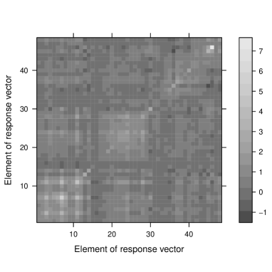
(a) Residual covariance matrix

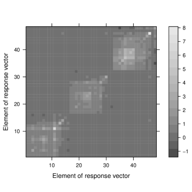
(b) Estimate with separable correlation

Figure 1: Estimated covariances for dissolved oxygen data. Opacity indicates covariance.

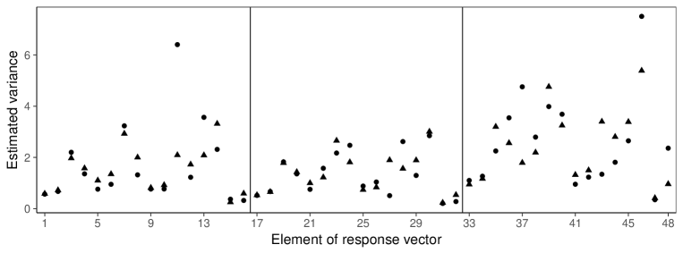
Figure 2: Estimated variances for dissolved oxygen data. Dots and triangles correspond to estimates from separable correlation and separable covariance models, respectively. The three panels are, from left to right, spring, summer, and fall.

7 Discussion

In settings where the data have a two-dimensional structure, the separable correlation model is a natural alternative to consider; it occupies a middle ground between separable and unstructured covariance.

By updating optimization variables in blocks and using rescaling we circumvent the need for more advanced, constrained optimization methods over sets of correlation matrices. Our algorithm also has closed form updates at every iteration, making it computationally convenient. Lu and Zimmerman, (2005) mention that the flip-flop algorithm is between 50 and 5000 times faster than a Newton–Raphson algorithm applied to their problem with separable covariance, and the difference increases with the dimension of the optimization problem. Given the similarities, we expect our algorithm to also outperform second order descent algorithms in terms of wall clock time, even though updating $W$ and rescaling $U$ and $V$ is more time-consuming in our model than in the separable covariance model. Our algorithm can be extended to handle constraints on the correlation matrices $U$ and $V$ by simply changing the corresponding update, without having to change anything else. Code for an R package (R Core Team,, 2018) implementing the proposed algorithm for fitting the separable correlation model is available at Ekvall, (2018).

Deriving analytical bounds for when minima exist and are unique in our model, similar to those in Soloveychik and Trushin, (2016), is an avenue for future research. Their proof does not immediately carry over to our setting since the negative log-likelihood of our model is not geodesically convex in the sense that of the separable covariance model is.

Further years of sampling would permit formal testing of the validity of the assumed separability against an unstructured covariance matrix in our data example. Restrictions on either the spatial or temporal autocorrelation could also be incorporated in such a study, building on the work of Szczepańska-Álvarez et al., (2017), as could the inclusion of habitat predictors and an analysis of how the assumed covariance structure affects inference about the regression coefficient $\beta$.

Supplementary material

The supplementary material includes proofs of propositions, additional simulation results, more details regarding the data example, and convergence diagnostics for the proposed algorithm.

References

- Cressie and Wikle, (2011) Cressie, N. and Wikle, C. K. (2011). Statistics for Spatio-Temporal Data. Wiley.
- Ding and Cook, (2017) Ding, S. and Cook, R. D. (2017). Matrix variate regressions and envelope models. Journal of the Royal Statistical Society: Series B (Statistical Methodology), 80(2):387–408.
- Dutilleul, (1999) Dutilleul, P. (1999). The MLE algorithm for the matrix normal distribution. Journal of Statistical Computation and Simulation, 64(2):105–123.
- Dutilleul and Pinel-Alloul, (1996) Dutilleul, P. and Pinel-Alloul, B. (1996). A doubly multivariate model for statistical analysis of spatio-temporal environmental data. Environmetrics, 7(6):551–565.
- Ekvall, (2018) Ekvall, K. O. (2018). kpcor. https://github.com/koekvall/kpcor.
- Fan et al., (2016) Fan, J., Liao, Y., and Liu, H. (2016). An overview of the estimation of large covariance and precision matrices. The Econometrics Journal, 19(1):C1–C32.
- Johnson and Hagerty, (2008) Johnson, B. L. and Hagerty, K. H. (2008). Status and trends of selected resources in the Upper Mississippi River system. techreport, U.S. Geological Survey, Upper Midwest Environmental Sciences Center. https://pubs.usgs.gov/mis/LTRMP2008-T002/pdf/LTRMP2008-T002_web.pdf (accessed 18 April 2018).
- Lu and Zimmerman, (2005) Lu, N. and Zimmerman, D. L. (2005). The likelihood ratio test for a separable covariance matrix. Statistics & Probability Letters, 73(4):449–457.
- Matsuda and Yajima, (2004) Matsuda, Y. and Yajima, Y. (2004). On testing for separable correlations of multivariate time series. Journal of Time Series Analysis, 25(4):501–528.
- R Core Team, (2018) R Core Team (2018). R: A Language and Environment for Statistical Computing. R Foundation for Statistical Computing, Vienna, Austria.
- Ren et al., (2013) Ren, C., Sun, D., and Sahu, S. K. (2013). Objective Bayesian analysis of spatial models with separable correlation functions. Canadian Journal of Statistics, 41(3):488–507.
- Rencher and Christensen, (2012) Rencher, A. C. and Christensen, W. F. (2012). Methods of Multivariate Analysis. Wiley.
- Soloveychik and Trushin, (2016) Soloveychik, I. and Trushin, D. (2016). Gaussian and robust Kronecker product covariance estimation: Existence and uniqueness. Journal of Multivariate Analysis, 149:92–113.
- Szczepańska-Álvarez et al., (2017) Szczepańska-Álvarez, A., Hao, C., Liang, Y., and von Rosen, D. (2017). Estimation equations for multivariate linear models with Kronecker structured covariance matrices. Communications in Statistics – Theory and Methods, 46(16):7902–7915.