The decay $h\to\gamma\gamma$ in the Standard-Model
Effective Field Theory

Abstract

Assuming that new physics effects are parametrized by the Standard-Model Effective Field Theory (SMEFT) written in a complete basis of up to dimension-6 operators, we calculate the CP-conserving one-loop amplitude for the decay $h\to\gamma\gamma$ in general $R_{\xi}$-gauges. We employ a simple renormalisation scheme that is hybrid between on-shell SM-like renormalised parameters and running $\overline{\mathrm{MS}}$ Wilson coefficients. The resulting amplitude is then finite, renormalisation scale invariant, independent of the gauge choice ($\xi$) and respects SM Ward identities. Remarkably, the $S$-matrix amplitude calculation resembles very closely the one usually known from renormalisable theories and can be automatised to a high degree. We use this gauge invariant amplitude and recent LHC data to check upon sensitivity to various Wilson coefficients entering from a more complete theory at the matching energy scale. We present a closed expression for the ratio $\mathcal{R}_{h\to\gamma\gamma}$, of the Beyond the SM versus the SM contributions as appeared in LHC $h\to\gamma\gamma$ searches. The most important contributions arise at tree level from the operators $Q_{\varphi B},Q_{\varphi W},Q_{\varphi WB}$, and at one-loop level from the dipole operators $Q_{uB},Q_{uW}$. Our calculation shows also that, for operators that appear at tree level in SMEFT, one-loop corrections can modify their contributions by less than 10%. Wilson coefficients corresponding to these five operators are bounded from current LHC $h\to\gamma\gamma$ data – in some cases an order of magnitude stronger than from other searches. Finally, we correct results that appeared previously in the literature.

1 Introduction

The discovery of the Higgs boson [1, 2, 3] in year 2012 was made possible mainly because of its decay into two photons [4, 5]. The current outcome for this decay channel from LHC (Run-2) with center-of-mass energy $\sqrt{s}=13\;\text{TeV}$, integrated luminosity of $36.1\;\text{fb}^{-1}$ and Higgs boson mass, $M_{h}=125.09\pm 0.24\;\text{GeV}$ is summarised as the ratio between the experimentally measured value (which may include contributions from new physics scenarios) relative to the Standard-Model (SM) predicted value [6, 7]

$$\mathcal{R}_{h\to\gamma\gamma}=\frac{\Gamma(\text{EXP},h\to\gamma\gamma)}{\Gamma(\text{SM},h\to\gamma\gamma)}\,.$$ (1.1)

The most recent measurements are presented by ATLAS [8] and CMS [9] experiments of LHC,

$$\text{ATLAS:}\qquad\mathcal{R}_{h\to\gamma\gamma} =0.99^{+0.15}_{-0.14}\,,$$

$$\text{CMS:}\qquad\mathcal{R}_{h\to\gamma\gamma} =1.18^{+0.17}_{-0.14}\,,$$ (1.2)

and are consistent with the SM prediction, with the error margin expected to be reduced in the near future.

If we consider the SM as a complete theory of electroweak (EW) and strong interactions up to the Planck scale, with no other scale involved in between, then the decay amplitude $h\to\gamma\gamma$ arises purely from dimension $d\leq 4$ (renormalisable) interactions. In this case the amplitude is finite, calculable and, since all relevant parameters are experimentally known, it is a certain prediction of the SM. It is this prediction entering the denominator in eq. (1.1). If however, there is New Physics beyond the SM already at a scale $\Lambda$ which is above, but not far from, the EW scale, say $\Lambda\sim{\cal O}(1-10)~{}\mathrm{TeV}$, then its effects can be parametrized by the presence of effective operators with dimension $d>4$ at scale $\Lambda$. These operators together with various parameters (or Wilson coefficients) will then run down to the EW scale and feed the on-shell scattering $S$-matrix amplitude together with $d\leq 4$ interactions.

All dimension $d\leq 6$ effective operators among SM particles that obey the SM gauge symmetry have been classified in refs. [10, 11]. The SM augmented with these effective operators – remnants of unknown heavy particles’ decoupling [12] – is called the SM Effective Field Theory, or for a short SMEFT. The quantization of SMEFT has recently been undertaken in ref. [13] in linear $R_{\xi}$-gauges with explicit proof of BRST symmetry and where all relevant primitive interaction vertices have been collected.

Within SM, numerous calculations for the $h\to\gamma\gamma$ amplitude exist. The first calculation was performed in ref. [6] in the limit of light Higgs mass ($M_{h}\ll M_{W}$), using dimensional regularisation in the ’t Hooft-Feynman gauge. Since then, there are other works completing this calculation in linear and non-linear gauges [14, 7, 15], with different regularisation schemes [16, 17, 18, 19, 20, 21, 22]. To our knowledge the complete SM one-loop $h\to\gamma\gamma$ amplitude in linear $R_{\xi}$-gauges is performed in ref. [23].

In SMEFT there is already a number of papers that calculate the $h\to\gamma\gamma$ amplitude [26, 27, 28, 29].^, The current, state of the art calculation, has been presented by Hartmann and Trott in refs. [33, 34]. The analysis was carried out using the Background Field Method (BFM) [35] consistent with minimal subtraction renormalisation scheme ($\overline{\mathrm{MS}}$) and included all relevant (CP-conserving) dimension $d\leq 6$ operators in calculating finite, non-log parts of the diagrams. Our work here is complementary but incorporates some additional features of importance:

• a simple calculational treatment in linear $R_{\xi}$-gauges based on Feynman rules of ref. [13],

• an analytical proof of gauge invariance (independence on the gauge choice $\xi$-parameter(s)) of the $S$-matrix element,

• a simple renormalisation framework which leads to a finite and renormalisation scale invariant amplitude,

• a compact semi-analytical expression highlighting the effect of new operators in the ratio $\mathcal{R}_{h\to\gamma\gamma}$ and corresponding bounds on Wilson coefficients.

There are quite a few papers addressing a global fit to the Higgs data from LHC Run-1 and Run-2 in the SMEFT framework [37, 38, 39]. Our work provides a simple semi-analytic one-loop formula for the ratio $\mathcal{R}_{h\to\gamma\gamma}$ in eq. (1.1) that can be used by these (usually tree level) fits or by analogous experimental analysis at LHC for Higgs boson searches.

Our paper is organised as follows. In section 2 we list operators contributing to the decay $h\to\gamma\gamma$ in SMEFT. Next, in section 3 we develop, in a pedagogical fashion, the renormalisation scheme for calculating the $h\to\gamma\gamma$ amplitude. In section 4 we give analytical expressions for all types of SM and SMEFT contributions to the $h\to\gamma\gamma$ amplitude and to the ratio $\mathcal{R}_{h\to\gamma\gamma}$. Semi-analytical prediction for $\mathcal{R}_{h\to\gamma\gamma}$, depending on the running Wilson coefficients and renormalisation scale $\mu$, are collected in section 5, and supplied with a discussion on numerical constraints of these coefficients. We conclude in section 6. Finally, in Appendix A we collect analytical expressions for the relevant one-loop self-energies and, relevant to $h\to\gamma\gamma$, three-point one-loop corrections in general $R_{\xi}$-gauges.

2 Relevant Operators

In EFT, an effect from the decoupling of heavy particles with masses of order $\Lambda$ is captured by the running parameters of the low energy theory influenced by higher dimensional operators added to SM renormalisable Lagrangian ${\cal L}_{\text{SM}}^{(4)}$. The full effective Lagrangian we consider here can be expressed as,

$${\cal L}={\cal L}_{\text{SM}}^{(4)}+\sum_{X}C^{X}Q_{X}^{(6)}+\sum_{f}C^{{}^{\prime}f}Q_{f}^{(6)}\,,$$ (2.1)

where $Q_{X}^{(6)}$ denotes dimension-6 operators that do not involve fermion fields, while $Q_{f}^{(6)}$ denotes operators that contain fermion fields. All Wilson coefficients should be rescaled by $\Lambda^{2}$, for example $C^{X}\to C^{X}/\Lambda^{2}$. We shall restore $1/\Lambda^{2}$ only in section 4 and thereafter. The prime in $C^{{}^{\prime}f}$, denotes a coefficient in flavour (“Warsaw”) basis of ref. [11] while we use unprimed coefficients in fermion mass basis defined in ref. [13].

$X^{3}$		$\varphi^{6}$  and  $\varphi^{4}D^{2}$		$\psi^{2}\varphi^{3}$
$Q_{W}$	$\varepsilon^{IJK}W_{\mu}^{I\nu}W_{\nu}^{J\rho}W_{\rho}^{K\mu}$	$Q_{\varphi}$	$(\varphi^{\dagger}\varphi)^{3}$	$Q_{e\varphi}$	$(\varphi^{\dagger}\varphi)(\bar{l}^{\prime}_{p}e^{\prime}_{r}\varphi)$
		$Q_{\varphi\Box}$	$(\varphi^{\dagger}\varphi)\raisebox{-1.42262pt}{$\Box$}(\varphi^{\dagger}\varphi)$	$Q_{u\varphi}$	$(\varphi^{\dagger}\varphi)(\bar{q}^{\prime}_{p}u^{\prime}_{r}\widetilde{\varphi})$
		$Q_{\varphi D}$	$\mathopen{}\mathclose{{}\left(\varphi^{\dagger}D^{\mu}\varphi}\right)^{*}\mathopen{}\mathclose{{}\left(\varphi^{\dagger}D_{\mu}\varphi}\right)$	$Q_{d\varphi}$	$(\varphi^{\dagger}\varphi)(\bar{q}^{\prime}_{p}d^{\prime}_{r}\varphi)$
$X^{2}\varphi^{2}$		$\psi^{2}X\varphi$		$\psi^{2}\varphi^{2}D$
$Q_{\varphi B}$	$\varphi^{\dagger}\varphi\,B_{\mu\nu}B^{\mu\nu}$	$Q_{eW}$	$(\bar{l}^{\prime}_{p}\sigma^{\mu\nu}e^{\prime}_{r})\tau^{I}\varphi W_{\mu\nu}^{I}$	$Q_{\varphi l}^{(3)}$	$(\mbox{${\varphi^{\dagger}i\,\raisebox{5.69054pt}{\boldmath${}^{\leftrightarrow}$}D_{\mu}^{\,I}\,\varphi}$})(\bar{l}^{\prime}_{p}\tau^{I}\gamma^{\mu}l^{\prime}_{r})$
$Q_{\varphi W}$	$\varphi^{\dagger}\varphi\,W^{I}_{\mu\nu}W^{I\mu\nu}$	$Q_{eB}$	$(\bar{l}^{\prime}_{p}\sigma^{\mu\nu}e^{\prime}_{r})\varphi B_{\mu\nu}$
$Q_{\varphi WB}$	$\varphi^{\dagger}\tau^{I}\varphi\,W^{I}_{\mu\nu}B^{\mu\nu}$	$Q_{uW}$	$(\bar{q}^{\prime}_{p}\sigma^{\mu\nu}u^{\prime}_{r})\tau^{I}\widetilde{\varphi}\,W_{\mu\nu}^{I}$
		$Q_{uB}$	$(\bar{q}^{\prime}_{p}\sigma^{\mu\nu}u^{\prime}_{r})\widetilde{\varphi}\,B_{\mu\nu}$
		$Q_{dW}$	$(\bar{q}^{\prime}_{p}\sigma^{\mu\nu}d^{\prime}_{r})\tau^{I}\varphi\,W_{\mu\nu}^{I}$
		$Q_{dB}$	$(\bar{q}^{\prime}_{p}\sigma^{\mu\nu}d^{\prime}_{r})\varphi\,B_{\mu\nu}$
		$\psi^{4}$
		$Q_{ll}$	$(\bar{l}^{\prime}_{p}\gamma_{\mu}l^{\prime}_{r})(\bar{l}^{\prime}_{s}\gamma^{\mu}l^{\prime}_{t})$

Table 1: A set of $d=6$ operators in Warsaw basis that contribute to the $h\to\gamma\gamma$ decay amplitude, directly or indirectly, in $R_{\xi}$-gauges. We consider only CP-conserving operators in our analysis. The operator $Q_{\varphi}$ cancels out completely in the $h\to\gamma\gamma$ amplitude. The operators $Q_{ll}$ and $Q_{\varphi l}^{(3)}$ present themselves indirectly through the translation of the renormalised vacuum expectation value (vev) into the well measured Fermi coupling constant, cf. eq. (3.5). The notation is the same as in refs. [11, 13]. For brevity we suppress fermion chiral indices $L,R$.

The operators involved in the calculation of decay $h\to\gamma\gamma$ are collected in Table 1. They can easily be identified when drawing the Feynman diagrams for $h\to\gamma\gamma$ looking at the primitive vertices listed in ref. [13]. There are 8 classes of such operators $X^{3},\varphi^{6},\varphi^{4}D^{2},\psi^{2}\varphi^{3},X^{2}\varphi^{2}$, $\psi^{2}X\varphi,\psi^{2}\varphi^{2}D,\psi^{4}$ where $X$ represents a gauge field strength tensor, $\varphi$ the Higgs doublet, $D$ a covariant derivative and $\psi$ a generic fermion field. Not counting flavour multiplicities and hermitian conjugation, in general, there are 16+2 CP-conserving operators. Actually, not all operators in Table 1 contribute in the final result for the $h\to\gamma\gamma$ amplitude. The operator $Q_{\varphi}$ cancels out completely after adding all contributions. This leaves 17 CP-conserving operators (or Wilson coefficients) relevant to the $h\to\gamma\gamma$ amplitude.

Another classification of various $d=6$ operators can be devised alongside with their strength [40, 41]. The division is between operators that are potentially tree level generated (PTG operators) and those that are loop generated (LG operators) by the more fundamental theory at high energies (UV-theory) under the assumption that the latter is perturbatively decoupled. Under this classification, operators relevant for $h\to\gamma\gamma$ amplitude are arranged as follows:

PTG	LG
$\varphi^{6}\;\text{and}\;\varphi^{4}D^{2}$	$X^{3}$
$\psi^{2}\varphi^{3}$	$X^{2}\varphi^{2}$
$\psi^{2}\varphi^{2}D$	$\psi^{2}X\varphi$
$\psi^{4}$

Table 2: PTG and LG classes of operators shown in Table 1.

LG operators are suppressed by $1/(4\pi)^{2}$ factors for each loop and may be thought to be sub-dominant corrections with respect to PTG operators. Relevant to $h\to\gamma\gamma$, PTG and LG classes of operators are listed in Table 2. On the other hand, a perturbative decoupling of the UV-theory may not necessarily be the case that Nature has chosen. In this work, although we do not assume any distinction amongst the $d=6$ operators involved in $h\to\gamma\gamma$ amplitude, we shall be referring to Table 2 as our analysis progresses.

3 Renormalisation

3.1 Parameter initialisation in SMEFT

There is a set of very well measured quantities, to which we rely upon, in relating our calculation for $\mathcal{R}_{h\to\gamma\gamma}$ to the LHC data. This set of experimental values is [42]

$$G_{F} =1.1663787(6)\times 10^{-5}\;\text{GeV}^{-2}\,,$$

$$\alpha_{\mathrm{EM}} =1/137.035999139(31)\quad\text{at}\;Q^{2}=0\,,$$

$$M_{W} =80.385(15)\;\text{GeV}\,,$$

$$M_{Z} =91.1876(21)\;\text{GeV}\,,$$

$$M_{h} =125.09\pm 0.24\;\text{GeV}\,,$$

$$m_{t} =173.1\pm 0.6\;\text{GeV}\,.$$ (3.1)

We identify these input values with the ones obtained in SMEFT consistent with the given accuracy of up to $1/\Lambda^{2}$ expansion terms. Consequently, following ref. [13] for the gauge and Higgs boson masses at tree level, it is enough to set $M_{W}$, $M_{Z}$ and $M_{h}$, respectively, equal to

$$M_{W} =\frac{1}{2}\bar{g}v\,,$$

$$M_{Z} =\frac{1}{2}\sqrt{\bar{g}^{2}+\bar{g}^{\prime 2}}v\mathopen{}\mathclose{{}\left(1+\frac{\bar{g}\bar{g}^{\prime}C^{\varphi WB}v^{2}}{\bar{g}^{2}+\bar{g}^{\prime 2}}+{1\over 4}C^{\varphi D}v^{2}}\right)\,,$$

$$M_{h}^{2} =\lambda v^{2}-\mathopen{}\mathclose{{}\left(3C^{\varphi}-2\lambda C^{\varphi\square}+\frac{\lambda}{2}C^{\varphi D}}\right)v^{4}\,,$$ (3.2)

where $\lambda$ is the Higgs quartic coupling, $\bar{g}^{\prime},\bar{g}$ are, respectively, the $U(1)_{Y}$ and $SU(2)_{L}$ gauge couplings (redefined to obtain canonical form of the gauge kinetic terms, see ref. [13]) and the $C$-coefficients correspond to operators defined in Table 1. Moreover, the fine-structure constant is identified through the Thomson limit ($Q^{2}=0$) as $\alpha_{\mathrm{EM}}=\bar{e}^{2}/4\pi$ where $\bar{e}$ is given at tree level by

$$\bar{e}=\frac{\bar{g}\bar{g}^{\prime}}{\sqrt{\bar{g}^{2}+\bar{g}^{\prime 2}}}\mathopen{}\mathclose{{}\left(1-\frac{\bar{g}\bar{g}^{\prime}}{\bar{g}^{2}+\bar{g}^{\prime 2}}\,C^{\varphi WB}\,v^{2}}\right)\,.$$ (3.3)

Similarly, the experimental values for lepton and quark masses, taken as pole masses from ref. [42], are equal to eqs. (3.27) and (3.29) of ref. [13].

The Fermi coupling constant $G_{F}$, is identified through the muon decay process. In addition to the $W$-boson exchange which is modified in SMEFT by the PMNS matrix that is (now) a non-unitary matrix containing the coefficient $C_{\varphi l}^{(3)}$, $G_{F}$ is also affected by dipole operators e.g., $Q_{eW}$ or by new diagrams with $Z$- or Higgs-boson exchange. However, the expression for $G_{F}$ is simplified by making the approximation of zero neutrino masses and also by assuming that

$$C_{1}\,{v^{2}}\gg C_{2}\,{v\,m_{l}}\,,$$ (3.4)

for any generic $C_{1}$ and $C_{2}$ coefficients entering the muon-decay amplitude and $m_{l}$ being a charged lepton mass. Only then we identify the Fermi coupling constant of eq. (3.1), within tree level in SMEFT, as

$$\frac{G_{F}}{\sqrt{2}}=\frac{\bar{G}_{F}}{\sqrt{2}}\mathopen{}\mathclose{{}\left[1+v^{2}(C_{11}^{\varphi l(3)}+C_{22}^{\varphi l(3)})-v^{2}C_{1221}^{ll}}\right]\,,\qquad\text{with}\quad\frac{\bar{G}_{F}}{\sqrt{2}}\equiv\frac{\bar{g}^{2}}{8M_{W}^{2}}=\frac{1}{2v^{2}}\,.$$ (3.5)

All Wilson coefficients entering in eq. (3.5) are real since they are diagonal elements of Hermitian matrices. In fact, and as a side test of the approximations assumed in eq. (3.4), we have checked that, at tree level in SMEFT, the full $S$-matrix element for the process $\mu^{-}\to e^{-}\bar{\nu}_{e}\nu_{\mu}$ is gauge invariant independently of lepton-number conservation. The formula (3.5) agrees with the corresponding one from refs. [24, 32].

3.2 Renormalisation framework

We ultimately want to bring the expression for the amplitude $\mathcal{A}(h\to\gamma\gamma)$, into a form that contains only renormalised parameters that are most closely related to observable quantities, the relevant ones given in eq. (3.1). At tree level in SMEFT, the $h\gamma\gamma$-vertex appears only in association with the unrenormalised (bare) Wilson coefficients, $C^{\varphi B}_{0},C^{\varphi W}_{0}$ and $C^{\varphi WB}_{0}$ and these are multiplied by the bare vev parameter $v_{0}$ (in what follows bare parameters are always denoted with a subscript zero). In order to set the stage, let us for example consider from Table 1 the $d=6$, CP-invariant operator of the form $X^{2}\varphi^{2}$,

$$C^{\varphi B}_{0}\,\varphi^{\dagger}\varphi\,B_{\mu\nu}\,B^{\mu\nu}\,,$$ (3.6)

where $\varphi$ is the scalar Higgs doublet and $B_{\mu\nu}$ is the $U(1)_{Y}$-hypercharge gauge field strength tensor. All fields and coupling constants are unrenormalised quantities in this expression. In what follows, and in order to keep the expressions as simple as possible, we keep working with unrenormalised fields i.e., no usual field redefinition is performed. This is justified, because we are interested in calculating only an on-shell $S$-matrix amplitude rather than a Green function.

After Spontaneous Symmetry Breaking (SSB) in SMEFT (see ref. [13] for details), the expression in eq. (3.6) contains the following term describing the interaction of the Higgs field and two “photons”,

$$C_{0}^{\varphi B}\,v_{0}\,h\,B_{\mu\nu}\,B^{\mu\nu}\,,$$ (3.7)

where $h$ is the Higgs field. We split these bare quantities into renormalised parameters $v,C^{\varphi B}$ and counterterms, $\delta v,\delta C^{\varphi B}$ respectively, as

$$v_{0}=v-\delta v\,,\qquad C^{\varphi B}_{0}=C^{\varphi B}-\delta C^{\varphi B}\,.$$ (3.8)

We follow the steps of a simple on-shell renormalisation scheme, first described in SM by Sirlin [46], and introduce new unrenormalised fields $A_{\mu}$ and $Z_{\mu}$ through the linear combinations

$$B_{\mu} =cA_{\mu}-sZ_{\mu}\,,$$ (3.9)

$$W_{\mu}^{3} =sA_{\mu}+cZ_{\mu}\,,$$ (3.10)

with $c\equiv\cos\theta_{W}$ and $s\equiv\sin\theta_{W}$ defined as a ratio of the physical masses of $W$ and $Z$ bosons, like

$$c^{2}\equiv\cos^{2}\theta_{W}=\frac{M_{W}^{2}}{M_{Z}^{2}}\,.$$ (3.11)

Therefore, the Lagrangian term for the considered operator, $Q_{\varphi B}$, describing (part of) the $h\gamma\gamma$ interaction, reads,

$$c^{2}\,v\,C^{\varphi B}\,\mathopen{}\mathclose{{}\left[1-\frac{\delta C^{\varphi B}}{C^{\varphi B}}-\frac{\delta v}{v}}\right]\,h\,F_{\mu\nu}F^{\mu\nu}\,.$$ (3.12)

Note that the vev counterterm arises from pure SM contributions because it multiplies $C^{\varphi B}$, while $\delta C^{\varphi B}$ cancels infinities that arise only from pure SMEFT diagrams i.e., in general, diagrams proportional to other $C$-coefficients, not necessarily only $C^{\varphi B}$.

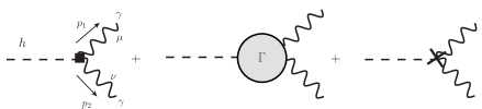
Figure 1: The sum of three types of diagrams: (left) the SMEFT “tree” contribution with momenta and space-time indices indicated, (center) the 1PI vertex corrections $\Gamma$ from all operators, SM or not, and (right) the vertex counterterms containing $\delta C$ and $\delta v$. These corrections should be self-explained in eq. (3.13).

Besides operator $Q_{\varphi B}$, counterterms for operators $Q_{\varphi W}$ and $Q_{\varphi WB}$ need to be added, too. Because all these three operators are proportional to the Higgs bilinear combination, $\varphi^{\dagger}\varphi$, they all contain the vev counterterm as a universal contribution to $h\to\gamma\gamma$ amplitude. The contributions discussed so far are depicted and explained in Fig. 1. By making use of the Feynman rules of ref. [13], their sum is written in momentum space, as

$$4i\,[\,p_{1}^{\nu}\,p_{2}^{\mu}-(p_{1}\cdot p_{2})\,g^{\mu\nu}\,]\,\Biggl{\{} c^{2}\,v\,C^{\varphi B}\mathopen{}\mathclose{{}\left[1+\Gamma^{\varphi B}-\frac{\delta C^{\varphi B}}{C^{\varphi B}}-\frac{\delta v}{v}}\right]$$

$$+s^{2}\,v\,C^{\varphi W}\mathopen{}\mathclose{{}\left[1+\Gamma^{\varphi W}-\frac{\delta C^{\varphi W}}{C^{\varphi W}}-\frac{\delta v}{v}}\right]$$

$$-sc\,v\,C^{\varphi WB}\mathopen{}\mathclose{{}\left[1+\Gamma^{\varphi WB}-\frac{\delta C^{\varphi WB}}{C^{\varphi WB}}-\frac{\delta v}{v}}\right]$$

$$+\frac{1}{M_{W}}\overline{\Gamma}^{\mathrm{SM}}+\sum_{X\neq\varphi B,\varphi W,\varphi WB}v\,C^{X}\,\Gamma^{X}\Biggr{\}}\,.$$ (3.13)

One-loop, 1PI vertex contributions proportional to $C^{\varphi B},C^{\varphi W}$ and $C^{\varphi WB}$ are denoted (up to pre-factors) with $\Gamma^{\varphi B},\Gamma^{\varphi W}$ and $\Gamma^{\varphi WB}$ in the first three lines of the above equation. The SM contribution, $\overline{\Gamma}^{\mathrm{SM}}$, is just the SM-famous result of ref. [6] but with the SM parameters replaced by the SMEFT ones (that is why “barred” $\Gamma$), taken from refs. [13, 47]. Furthermore, there are additional one-loop corrections, $\Gamma^{X}$, proportional to Wilson coefficients $C^{X}$, like for instance $C^{W}$, which are collected in the last line, last term of eq. (3.13).

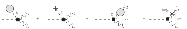
Figure 2: Tadpole and $Z\gamma$ self-energy contributions with their associated counterterms. Crosses denote SM counterterms and the black boxes indicate pure $d=6$ operator insertions.

There are additional diagrams participating in the $h\to\gamma\gamma$ amputated amplitude. These are shown in Fig. 2. The first two classes of diagrams are the Higgs tadpole and its counterterm contributions. These two diagrams do not enter in our renormalised amplitude because, following the renormalisation scheme of ref. [48], the Higgs tadpole counterterm is adjusted to cancel the 1PI Higgs tadpole diagrams. This guarantees that the vev is unchanged to one-loop order. The last two diagrams in Fig. 2 represent the $Z\gamma$-self energy at $p^{2}=0$, $A_{Z\gamma}(0)$, plus its counterterm, $\delta m_{Z\gamma}^{2}$. The expression for the counterterm $\delta m^{2}_{Z\gamma}$ (given below) is gauge invariant independently of the renormalisation condition for the Higgs tadpole. This is practically very useful for proving the gauge invariance of the $h\to\gamma\gamma$ amplitude.

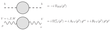
Figure 3: Definitions for Higgs and vector boson ($V=\gamma,Z,W$), 1PI self-energies.

Finally, as usual, by multiplying the amputated graph with the LSZ-factors [49] (see for instance section 7.2 of textbook [50]) for the external Higgs and photon fields,

$$\sqrt{Z_{hh}}\,Z_{\gamma\gamma}=1+\frac{1}{2}\Pi_{HH}^{\prime}(M_{h}^{2})-\Pi_{\gamma\gamma}(0)\,,$$ (3.14)

we arrive at the following $S$-matrix amplitude:

$$i\mathcal{A}^{\mu\nu}(h\to\gamma\gamma)=\langle\gamma(\epsilon^{\mu},p_{1}),\,\gamma(\epsilon^{\nu},p_{2})\,|\,S\,|\,h(q)\,\rangle=4i\,\mathopen{}\mathclose{{}\left[\,p_{1}^{\nu}\,p_{2}^{\mu}-(p_{1}\cdot p_{2})\,g^{\mu\nu}\,}\right]\times$$

$$\Biggl{\{}c^{2}\,v\,C^{\varphi B}\mathopen{}\mathclose{{}\left[1+\Gamma^{\varphi B}-\frac{\delta C^{\varphi B}}{C^{\varphi B}}-\frac{\delta v}{v}+\frac{1}{2}\Pi_{HH}^{\prime}(M_{h}^{2})-\Pi_{\gamma\gamma}(0)+2\tan\theta_{W}\frac{A_{Z\gamma}(0)+\delta m^{2}_{Z\gamma}}{M_{Z}^{2}}}\right]$$

$$+s^{2}\,v\,C^{\varphi W}\mathopen{}\mathclose{{}\left[1+\Gamma^{\varphi W}-\frac{\delta C^{\varphi W}}{C^{\varphi W}}-\frac{\delta v}{v}+\frac{1}{2}\Pi_{HH}^{\prime}(M_{h}^{2})-\Pi_{\gamma\gamma}(0)-\frac{2}{\tan\theta_{W}}\frac{A_{Z\gamma}(0)+\delta m^{2}_{Z\gamma}}{M_{Z}^{2}}}\right]$$

$$-sc\,v\,C^{\varphi WB}\mathopen{}\mathclose{{}\left[1+\Gamma^{\varphi WB}-\frac{\delta C^{\varphi WB}}{C^{\varphi WB}}-\frac{\delta v}{v}+\frac{1}{2}\Pi_{HH}^{\prime}(M_{h}^{2})-\Pi_{\gamma\gamma}(0)-\frac{2}{\tan 2\theta_{W}}\frac{A_{Z\gamma}(0)+\delta m^{2}_{Z\gamma}}{M_{Z}^{2}}}\right]$$

$$+\frac{1}{M_{W}}\overline{\Gamma}^{\mathrm{SM}}+\sum_{X\neq\varphi B,\varphi W,\varphi WB}\,v\,C^{X}\,\Gamma^{X}\Biggr{\}}\,.$$ (3.15)

Eq. (3.15) is our master formula for the renormalised amplitude $\mathcal{A}^{\mu\nu}(h\to\gamma\gamma)$. The definitions for the various self-energies are stated in Fig. 3 and

$$\Pi^{\prime}_{HH}(M_{h}^{2})\equiv\frac{\partial\Pi_{HH}(p^{2})}{\partial p^{2}}\biggr{|}_{p^{2}=M_{h}^{2}}\,,\qquad A_{\gamma\gamma}(p^{2})=-p^{2}\,\Pi_{\gamma\gamma}(p^{2})+\mathcal{O}(\alpha_{\mathrm{EM}}^{2})\,,$$ (3.16)

where $\Pi_{\gamma\gamma}(p^{2})$ is regular at $p^{2}=0$. All self-energies in eq. (3.15) should arise purely from SM diagrams because we are including terms up to $1/\Lambda^{2}$ in SMEFT. As noted earlier, the SM counterterm, $\delta m^{2}_{Z\gamma}$, is gauge invariant and is given by [46]:

$$\frac{\delta m^{2}_{Z\gamma}}{M_{Z}^{2}}=\frac{1}{2\tan\theta_{W}}\operatorname{Re}\mathopen{}\mathclose{{}\left[\frac{A_{ZZ}(M_{Z}^{2})}{M_{Z}^{2}}-\frac{A_{WW}(M_{W}^{2})}{M_{W}^{2}}}\right]\,.$$ (3.17)

The quantity $\delta v/v$ is not gauge invariant. Following standard on-shell renormalisation conditions of refs. [46, 48], we write

$$\frac{\delta v}{v}=\operatorname{Re}\mathopen{}\mathclose{{}\left[\frac{A_{WW}(M_{W}^{2})}{2M_{W}^{2}}}\right]-\frac{\delta g}{g}\,,$$ (3.18)

where the counterterm $\delta g$ of the $SU(2)_{L}$ gauge coupling is gauge invariant and reads as

$$\frac{\delta g}{g}=\frac{\delta e}{e}-\frac{1}{\tan\theta_{W}}\,\frac{\delta m^{2}_{Z\gamma}}{M_{Z}^{2}}\,.$$ (3.19)

Here $\delta e$ is the electromagnetic charge renormalisation counterterm which is also gauge invariant. This is given by eq. (26) of ref. [46]

$$\frac{\delta e}{e}=-\frac{1}{2}\Pi^{\mathrm{lept}}_{\gamma\gamma}(0)-\frac{1}{2}\Pi^{\mathrm{had}}_{\gamma\gamma}(0)+\frac{7e^{2}}{32\pi^{2}}\mathopen{}\mathclose{{}\left[\mathopen{}\mathclose{{}\left(\frac{2}{\epsilon}-\gamma+\log 4\pi}\right)-\log\frac{M_{W}^{2}}{\mu^{2}}+\frac{2}{21}}\right]\,,$$ (3.20)

where $\mu$ is the renormalisation scale parameter and $\epsilon\equiv 4-d$. Leptonic and hadronic contributions, $\Pi^{\mathrm{lept}}_{\gamma\gamma}(0)$ and $\Pi^{\mathrm{had}}_{\gamma\gamma}(0)$, to the photon vacuum polarisation are gauge invariant and the infinite part in the squared brackets should be gauge invariant too. The hadronic contribution from light quarks, $\Pi^{\mathrm{had}}_{\gamma\gamma}(0)$, is in principle non-calculable due to strong interaction at zero momenta. A dispersive or other non-perturbative methods should be in order. There is no such problem of course with $\Pi^{\mathrm{lept}}_{\gamma\gamma}(0)$.

SM vector boson self-energy contributions can be found in ref. [51]. The Higgs self-energy contribution can be found in refs. [48, 34]. These results have been obtained in the particular case of the ’t Hooft-Feynman gauge where $\xi=1$. Thanks to the set of SMEFT Feynman Rules in general $R_{\xi}$-gauges [13], we present in Appendix A all contributions needed in eq. (3.15) with the explicit $\xi$-dependence. This is necessary for checking the gauge invariance of the amplitude. Finally, the counterterms $\delta C^{\varphi B},\delta C^{\varphi W}$ and $\delta C^{\varphi WB}$ can be read from refs. [27, 52, 53, 47, 34, 33] where they have been calculated again in ’t Hooft-Feynman ($\xi=1$) gauge. However, in $\overline{\mathrm{MS}}$ renormalisation scheme and at one-loop, cancellation of infinities should be independent on the gauge choice as we confirm below.

3.3 $\xi$-independence

Knowing the gauge invariant and non-invariant parts of various contributions, as described above, is particularly useful for proving the $\xi$-independence of the amplitude. We first prove gauge invariance by means of $\xi$-independence for the infinite parts proportional to $\xi_{W}$ or $\xi_{Z}$. We find that the combination of $\delta v/v$ and $\Pi_{HH}^{\prime}(M_{h}^{2})$ in eq. (3.15) is $\xi$-independent. For the $C^{\varphi B}$ contribution in eq. (3.15), the $\xi_{W}$-dependent terms inside $\Pi_{\gamma\gamma}(0)$ and $A_{Z\gamma}(0)$ cancel among each other, as they should since the infinite part of $\Gamma^{\varphi B}$ is $\xi$-independent by itself. For contributions proportional to $C^{\varphi W}$ ($C^{\varphi WB}$), the $\xi_{W}$ cancellations take place throughout the self-energy contributions and $\Gamma^{\varphi W}$ ($\Gamma^{\varphi WB}$). Furthermore, diagrams proportional to $C^{X}$ with $X\neq\varphi B,\varphi W,\varphi WB$, contributing to the last term of eq. (3.15), are gauge invariant on their own. Of course $\overline{\Gamma}^{\mathrm{SM}}$ is finite and gauge invariant as it is known from a direct calculation in $R_{\xi}$-gauges with dimensional regularisation [23].

We then prove analytically the cancellation of all $\xi$-dependent finite parts. This was done by first performing a maximal reduction on the related Passarino-Veltman functions [54] and then analytically checking for $\xi$-dependence among the parametric integrals. This is a highly non-trivial check of the validity of our calculation because the gauge parameter $\xi$ appears everywhere in both the SM and SMEFT contributions which are directly related to the $h\to\gamma\gamma$ amplitude. Moreover, this should be also considered as a direct proof for the validity of the expressions for vertices given in ref. [13] in general $R_{\xi}$-gauges. Most importantly, the $\xi$-cancellation shows that the amplitude $\mathcal{A}^{\mu\nu}(h\to\gamma\gamma)$ given in eq. (3.15) is gauge invariant as it should be. Needless to say, this is a very encouraging indication towards the correctness of our final result.

As an additional non-trivial check of our calculation, we have also proved gauge invariance for our amplitude before adopting any renormalisation scheme. We confirm that the regularised but yet unrenormalised $S$-matrix amplitude for $h\to\gamma\gamma$, written in terms of bare parameters, is gauge invariant.

3.4 $\overline{\mathrm{MS}}$ scheme for Wilson coefficients

All renormalised coefficients, say $C$, and the counterterms, $\delta C$, in eq. (3.15), can be readily written in terms of the $\overline{\mathrm{MS}}$-scheme running $C$-coefficients as

$$C-\delta C=\bar{C}(\mu)-\delta\bar{C}\,,$$ (3.21)

where $\mu$ is the renormalisation (or subtraction) scale that lays somewhere between the EW scale and the scale $\Lambda$, while $\delta\bar{C}$ is a counterterm that subtracts only terms proportional to

$$E\equiv\frac{2}{\epsilon}-\gamma+\log 4\pi\,,\quad\mathrm{with}\quad\epsilon\equiv 4-d\,,$$ (3.22)

in the loop corrections for the Wilson $C$-coefficients. In $\overline{\mathrm{MS}}$ scheme and at one-loop, these counterterms are independent of the choice of the gauge fixing and can be read directly from refs. [52, 47, 53] to be

$$\delta\bar{C}^{\varphi B}=\frac{E}{16\pi^{2}}\Biggl{\{} \biggl{(}-3\lambda-Y+\frac{9}{4}\bar{g}^{2}-\frac{85}{12}\bar{g}^{\prime 2}\biggr{)}C^{\varphi B}-\frac{3}{2}\bar{g}\bar{g}^{\prime}C^{\varphi WB}$$

$$-\mathopen{}\mathclose{{}\left[\frac{3}{2}\bar{g}^{\prime}\operatorname{Tr}(C^{\prime eB}\Gamma_{e}^{\dagger})-\frac{5}{6}\bar{g}^{\prime}N_{c}\operatorname{Tr}(C^{\prime uB}\Gamma_{u}^{\dagger})+\frac{1}{6}\bar{g}^{\prime}N_{c}\operatorname{Tr}(C^{\prime dB}\Gamma_{d}^{\dagger})+\mathrm{H.c.}}\right]\Biggr{\}}\,,$$ (3.23)

$$\delta\bar{C}^{\varphi W}=\frac{E}{16\pi^{2}}\Biggl{\{} \Biggl{(}-3\lambda-Y+\frac{53}{12}\bar{g}^{2}+\frac{3}{4}\bar{g}^{\prime 2}\Biggr{)}C^{\varphi W}-\frac{1}{2}\bar{g}\bar{g}^{\prime}C^{\varphi WB}+\frac{15}{2}\bar{g}^{3}C^{W}$$

$$+\mathopen{}\mathclose{{}\left[\frac{1}{2}\bar{g}\,\operatorname{Tr}(C^{\prime eW}\Gamma_{e}^{\dagger})+\frac{1}{2}\bar{g}\,N_{c}\operatorname{Tr}(C^{\prime uW}\Gamma_{u}^{\dagger})+\frac{1}{2}\bar{g}\,N_{c}\operatorname{Tr}(C^{\prime dW}\Gamma_{d}^{\dagger})+\mathrm{H.c.}}\right]\Biggr{\}}\,,$$ (3.24)

$${\delta\bar{C}^{\varphi WB}}=\frac{E}{16\pi^{2}}\Biggl{\{} \Biggl{(}-\lambda-Y-\frac{2}{3}\bar{g}^{2}-\frac{19}{6}\bar{g}^{\prime 2}\Biggr{)}C^{\varphi WB}-\bar{g}\bar{g}^{\prime}(C^{\varphi B}+C^{\varphi W})-\frac{3}{2}\bar{g}^{\prime}\bar{g}^{2}C^{W}$$

$$+\mathopen{}\mathclose{{}\left[\frac{1}{2}\bar{g}\,\operatorname{Tr}(C^{\prime eB}\Gamma_{e}^{\dagger})-\frac{1}{2}\bar{g}\,N_{c}\operatorname{Tr}(C^{\prime uB}\Gamma_{u}^{\dagger})+\frac{1}{2}\bar{g}\,N_{c}\operatorname{Tr}(C^{\prime dB}\Gamma_{d}^{\dagger})}\right.$$

$$\mathopen{}\mathclose{{}\left.-\frac{3}{2}\bar{g}^{\prime}\operatorname{Tr}(C^{\prime eW}\Gamma_{e}^{\dagger})-\frac{5}{6}\bar{g}^{\prime}N_{c}\operatorname{Tr}(C^{\prime uW}\Gamma_{u}^{\dagger})-\frac{1}{6}\bar{g}^{\prime}N_{c}\operatorname{Tr}(C^{\prime dW}\Gamma_{d}^{\dagger})+\mathrm{H.c.}}\right]\Biggr{\}}\,,$$ (3.25)

where $\Gamma_{u,d,e}$ is our notation [11, 13] for the usual Yukawa couplings in SM, and using Table 4 from ref. [13], the coefficients $C^{\prime\,f}$ are rotated to the fermion mass basis (denoted now as unprimed ones), and

$$Y\equiv\frac{2}{v^{2}}\sum_{i=1}^{3}(m_{e_{i}}^{2}+N_{c}m_{d_{i}}^{2}+N_{c}m_{u_{i}}^{2})\,,\qquad\operatorname{Tr}(C^{\prime eB}\Gamma_{e}^{\dagger})=\frac{\sqrt{2}}{v}C^{eB}_{ii}m_{e_{i}}\,,\quad\text{etc.}$$ (3.26)

$N_{c}=3$ is the number of colours and $m_{f_{i}}$ a mass of the SM fermion belonging to the $i$-th generation. All $C$-coefficients have been taken real. We have checked explicitly and analytically that the counterterms of eqs. (3.23), (3.24) and (3.25) render the amplitude for $h\to\gamma\gamma$ of eq. (3.15) finite, at one-loop and up to $1/\Lambda^{2}$ in EFT expansion.

3.5 The amplitude

The remaining part of $\mathcal{A}^{\mu\nu}(h\to\gamma\gamma)$ in eq. (3.15) is, at one-loop and up to $1/\Lambda^{2}$ terms, renormalisation scale invariant: the renormalisation group running of $\bar{C}(\mu)$ coefficients cancels the explicit $\mu$-dependence within various contributions in the RHS of eq. (3.15). Therefore, the amplitude, to be squared in finding the $h\to\gamma\gamma$ decay width, is

$$i\mathcal{A}^{\mu\nu}(h\to\gamma\gamma)=\langle\gamma(\epsilon^{\mu},p_{1}),\,\gamma(\epsilon^{\nu},p_{2})\,|\,S\,|\,h(q)\,\rangle=4i\,\mathopen{}\mathclose{{}\left[\,p_{1}^{\nu}\,p_{2}^{\mu}-(p_{1}\cdot p_{2})\,g^{\mu\nu}\,}\right]\,\mathcal{A}_{h\to\gamma\gamma}\,,$$ (3.27)

where

$$\mathcal{A}_{h\to\gamma\gamma} =\Biggl{\{}c^{2}\,v\,\bar{C}^{\varphi B}(\mu)\mathopen{}\mathclose{{}\left[1+\Gamma^{\varphi B}-\frac{\delta v}{v}+\frac{1}{2}\Pi_{HH}^{\prime}(M_{h}^{2})-\Pi_{\gamma\gamma}(0)+2\tan\theta_{W}\frac{A_{Z\gamma}(0)+\delta m^{2}_{Z\gamma}}{M_{Z}^{2}}}\right]$$

$$\qquad+s^{2}\,v\,\bar{C}^{\varphi W}(\mu)\mathopen{}\mathclose{{}\left[1+\Gamma^{\varphi W}-\frac{\delta v}{v}+\frac{1}{2}\Pi_{HH}^{\prime}(M_{h}^{2})-\Pi_{\gamma\gamma}(0)-\frac{2}{\tan\theta_{W}}\frac{A_{Z\gamma}(0)+\delta m^{2}_{Z\gamma}}{M_{Z}^{2}}}\right]$$

$$\qquad-sc\,v\,\bar{C}^{\varphi WB}(\mu)\mathopen{}\mathclose{{}\left[1+\Gamma^{\varphi WB}-\frac{\delta v}{v}+\frac{1}{2}\Pi_{HH}^{\prime}(M_{h}^{2})-\Pi_{\gamma\gamma}(0)-\frac{2}{\tan 2\theta_{W}}\frac{A_{Z\gamma}(0)+\delta m^{2}_{Z\gamma}}{M_{Z}^{2}}}\right]$$

$$\qquad+\frac{1}{M_{W}}\overline{\Gamma}^{\mathrm{SM}}+\ \sum_{X\neq\varphi B,\varphi W,\varphi WB}\,v\,C^{X}(\mu)\,\Gamma^{X}\,\Biggr{\}}_{\mathrm{finite}}\,.$$ (3.28)

The subscript “finite” in the final parenthesis means that infinities proportional to $E$ have been subtracted from all contributions in eq. (3.28) such as $\Gamma$, $\Pi^{\prime}_{HH}$, $\Pi_{VV}$, $A_{VV}$, etc. The $\mathcal{A}_{h\to\gamma\gamma}$ in eq. (3.28) is finite, gauge and renormalisation scale invariant as a physical amplitude must be. In eq. (3.28), $\Gamma^{\varphi B}$, $\Gamma^{\varphi W}$ and $\Gamma^{\varphi WB}$ are given in Appendix A in eqs. (A), (A) and (A). The quantities ${\delta v}/{v}$ and ${\delta m^{2}_{Z\gamma}}/{M_{Z}^{2}}$ are presented in eqs. (3.18) and (3.17), respectively. All vector boson self-energies in general $R_{\xi}$-gauges as well as the quantity $\Pi_{HH}^{\prime}(M_{h}^{2})$ are also given in Appendix A.

Although all $\bar{C}(\mu)$ coefficients in eq. (3.28) are $\overline{\mathrm{MS}}$ parameters, the weak mixing angle $\theta_{W}$ and the vev $v$ that appear explicitly to multiply Wilson coefficients are defined in terms of physical quantities through eqs. (3.11) and (3.5) [see also eq. (4.16) below]. This is a virtue of our hybrid renormalisation scheme: SM on-shell parameters appear together with $\overline{\mathrm{MS}}$ SMEFT parameters (Wilson coefficients) in the renormalised amplitude. This scheme can easily be applied to every process at one-loop in SMEFT.

From now on, all Wilson coefficients should be considered as running $\overline{\mathrm{MS}}$ quantities, $C\equiv\bar{C}(\mu)$. We remove the “bar” over the $\overline{\mathrm{MS}}$-coefficients letting the argument to denote, or to implicitly imply, the difference.

4 Anatomy of the effective amplitude

In this section we present explicit expressions for the SM contribution, and, contributions proportional to all Wilson coefficients entering the $h\to\gamma\gamma$ amplitude in eq. (3.28), and in Table 1. These coefficients are taken to be real. For clarity, we reinstate explicitly $1/\Lambda^{2}$ factors in the expressions appeared in this and subsequent sections, so they are no longer incorporated into the definition of $C$’s. Our EFT expansion stops at the order $1/\Lambda^{2}$ and is one-loop at the $\hbar$-expansion. In our conventions, we denote electromagnetic fermion charges and the third component of particle weak isospin as

$$Q_{f}=\begin{cases}0,&\text{for}\quad f=\nu_{e},\nu_{\mu},\nu_{\tau}\\ -1,&\text{for}\quad f=e,\mu,\tau\\ 2/3,&\text{for}\quad f=u,c,t\\ -1/3,\;&\text{for}\quad f=d,s,b\\ \end{cases}\quad\text{and}\quad T_{f}^{3}=\begin{cases}1/2,&\text{for}\quad f=\nu_{e},\nu_{\mu},\nu_{\tau},u,c,t\\ -1/2,\;&\text{for}\quad f=e,\mu,\tau,d,s,b\end{cases}\,.$$ (4.1)

The colour factors are $N_{c,e}=1$ and $N_{c,u}=N_{c,d}=3$. It is useful to note, when reading the expressions below, that the actual dimensionless EFT expansion parameter is $\frac{1}{G_{F}\Lambda^{2}}$. To get a quantitative feeling of its numerical magnitude and to compare with standard loop expansion in the EW gauge couplings, we simply note that it is $\frac{1}{G_{F}M_{W}^{2}}\sim 4\pi$, while for $\Lambda=1~{}\mathrm{TeV}$ one has $\frac{1}{G_{F}\Lambda^{2}}\sim\frac{1}{4\pi}$, for $\Lambda=10~{}\mathrm{TeV}$ one has $\frac{1}{G_{F}\Lambda^{2}}\sim\frac{\alpha_{\mathrm{EM}}}{4\pi}$ and, finally, for $\Lambda=100~{}\mathrm{TeV}$ one has $\frac{1}{G_{F}\Lambda^{2}}\sim\frac{\alpha^{2}_{\mathrm{EM}}}{\pi^{2}}$.

4.1 SM and $C^{\varphi WB}$, $C^{\varphi l(3)}$, $C^{ll}$

The famous “SM” contributions from $W$ and fermion triangle loops are represented by the penultimate term in eq. (3.28). This is

$$\frac{\overline{\Gamma}^{\mathrm{SM}}}{M_{W}}=\frac{1}{64\pi^{2}}\frac{\bar{g}^{2}\bar{g}^{\prime 2}}{(\bar{g}^{2}+\bar{g}^{\prime 2})}\frac{\bar{g}}{M_{W}}I_{\gamma\gamma}\,,$$ (4.2)

with

$$I_{\gamma\gamma}\equiv I_{\gamma\gamma}(r_{f},r_{W})=\sum_{f}Q_{f}^{2}N_{c,f}A_{1/2}(r_{f})-A_{1}(r_{W})\,,$$ (4.3)

and

$$A_{1/2}(r_{f}) =2r_{f}\mathopen{}\mathclose{{}\left[1+(1-r_{f})f(r_{f})}\right]\,,$$ (4.4)

$$A_{1}(r_{W}) =2+3r_{W}\mathopen{}\mathclose{{}\left[1+(2-r_{W})f(r_{W})}\right]\,.$$ (4.5)

Here $Q_{f}$ and $m_{f}$ are the fermion charge (in the units of proton charge), and mass, respectively, $N_{c,f}$ is the colour factor for fermions (3 for quarks, 1 for leptons) and

$$r_{f}\equiv\frac{4m_{f}^{2}}{M_{h}^{2}}\,,\qquad r_{W}\equiv\frac{4M_{W}^{2}}{M_{h}^{2}}\,.$$ (4.6)

The result is of course finite and is governed by a single function $f(r)$, which reads

$$f(r)=\begin{cases}\arcsin^{2}\mathopen{}\mathclose{{}\left(\frac{1}{\sqrt{r}}}\right)\,,\quad r\geq 1\,,\\ -\frac{1}{4}\mathopen{}\mathclose{{}\left[\log\mathopen{}\mathclose{{}\left(\frac{1+\sqrt{1-r}}{1-\sqrt{1-r}}}\right)-i\pi}\right]^{2}\,,\quad r\leq 1\,.\end{cases}$$ (4.7)

It is useful for order of magnitude calculations to state that $A_{1}(r_{W})\approx 8.33$, $A_{1/2}(r_{t})\approx 1.38$ and $I_{\gamma\gamma}\approx-6.56$ with a negligible imaginary part.

The expression given in eq. (4.2) is not exactly the SM contribution for it is written in terms of SMEFT parameters and not in terms of measurable quantities like those listed in eq. (3.1). We therefore rewrite eq. (4.2) in terms of physical quantities using the expression for $\bar{e}$ from eq. (3.3) and $G_{F}$ from eq. (3.5) that bring in the new coefficients $C^{\varphi WB}$ and $C_{11}^{\varphi l(3)},C_{22}^{\varphi l(3)},C_{1221}^{ll}$, respectively,

$$\frac{\overline{\Gamma}^{\mathrm{SM}}}{M_{W}}=\frac{\alpha_{EM}}{16\pi}\mathopen{}\mathclose{{}\left(\frac{8G_{F}}{\sqrt{2}}}\right)^{1/2}I_{\gamma\gamma}\mathopen{}\mathclose{{}\left[1+2sc\,\frac{v^{2}}{{\Lambda^{2}}}C^{\varphi WB}-\frac{v^{2}}{2{\Lambda^{2}}}(C_{11}^{\varphi l(3)}+C_{22}^{\varphi l(3)})+\frac{v^{2}}{2{\Lambda^{2}}}C_{1221}^{ll}}\right]\,.$$ (4.8)

Note that the piece before the square brackets on the RHS is the SM contribution to amplitude [up to a Lorentz factor in eq. (3.27)], as it would be calculated in the absence of any higher order operators. Inside the square brackets there are contributions from SMEFT i.e., running Wilson coefficients evaluated at a scale $\mu$. Hence, the precise determination of the $\mathcal{R}_{h\to\gamma\gamma}$ in eq. (1.1) is

$$\mathcal{R}_{h\to\gamma\gamma}=\frac{\Gamma(\mathrm{SMEFT},h\to\gamma\gamma)}{\Gamma(\mathrm{SM},h\to\gamma\gamma)}\equiv 1+\delta\mathcal{R}_{h\to\gamma\gamma}\,,$$ (4.9)

where the SM decay width reads, in accordance with standard refs. [55, 56, 23], as

$$\Gamma(\mathrm{SM},h\to\gamma\gamma)=\frac{G_{F}\,\alpha_{\mathrm{EM}}^{2}\,M_{h}^{3}}{128\sqrt{2}\pi^{3}}\,|I_{\gamma\gamma}|^{2}\,,$$ (4.10)

with $I_{\gamma\gamma}$ given in eq. (4.3). The SMEFT contributions of eq. (4.8) are encoded in a part of $\delta\mathcal{R}_{h\to\gamma\gamma}$ of eq. (4.9), in terms of measurable quantities $s,c$ and $G_{F}$, as

$$\delta\mathcal{R}_{h\to\gamma\gamma}^{(1)}\simeq\frac{4sc}{\sqrt{2}}\frac{1}{G_{F}\Lambda^{2}}C^{\varphi WB}-\frac{1}{\sqrt{2}}\frac{1}{G_{F}\Lambda^{2}}(C_{11}^{\varphi\ell(3)}+C_{22}^{\varphi\ell(3)})+\frac{1}{\sqrt{2}}\frac{1}{G_{F}\Lambda^{2}}C_{1221}^{\ell\ell}\,,$$ (4.11)

where $c^{2}=1-s^{2}=M_{W}^{2}/M_{Z}^{2}$. Following our EFT expansion assumption, in obtaining eq. (4.11), corrections of $\mathcal{O}(1/\Lambda^{4})$ have been consistently ignored.

4.2 $C^{\varphi D}$, $C^{\varphi\Box}$, $C^{\varphi}$

A direct calculation shows that the contribution from operators $C^{\varphi\Box}$ and $C^{\varphi D}$ is simply

$$\mathopen{}\mathclose{{}\left(1+{\frac{v^{2}}{\Lambda^{2}}}C^{\varphi\Box}-{\frac{v^{2}}{4\Lambda^{2}}}C^{\varphi D}}\right)(i\mathcal{A}^{\mathrm{SM}})\equiv Z_{h}^{-1}(i\mathcal{A}^{\mathrm{SM}})\,,$$ (4.12)

where $Z_{h}$ is the field redefinition factor for making the kinetic term of the Higgs field canonical in going from SM to SMEFT (see eq.(3.5) of ref. [13]) and $i\mathcal{A}^{\mathrm{SM}}$ is the full SM contribution to $h\to\gamma\gamma$ amplitude. There is an explanation for this result based on the quantization of SMEFT presented in ref. [13]. In unitary gauge these operators appear in Higgs boson vertices ($hWW$ and $hff$) with exactly the same Lorentz structure as in the corresponding SM vertices. On the other hand, in “renormalisable” gauges these operators appear in a complicated way e.g., there are contributions from Goldstone bosons $hG^{0}G^{0}$ that have a non-trivial, non-SM Lorentz structure [13] and eq. (4.12) is not easily seen without performing the actual calculation. However, the result should be independent on the gauge choice as we explicitly confirm. We can view eq. (4.12) in a different way starting from the SM amplitude and perform the redefinition $H=Z_{h}^{-1}h$ on the single external Higgs boson leg.

As we already mentioned in section 2, the coefficient $C^{\varphi}$ does not contribute explicitly to the $h\to\gamma\gamma$ amplitude in unitary gauge. Although there are apparent non-trivial contributions from it to vertices in $R_{\xi}$-gauges, once again, gauge invariance implies that the amplitude is explicitly independent of $C^{\varphi}$. Again, we explicitly verify this situation as well.

In summary, the contribution of operators discussed in this subsection to the ratio (4.9) reads trivially, up to $\sim 1/\Lambda^{2}$ terms, as

$$\delta\mathcal{R}_{h\to\gamma\gamma}^{(2)}\simeq\sqrt{2}\frac{1}{G_{F}\Lambda^{2}}C^{\varphi\Box}-\frac{\sqrt{2}}{4}\frac{1}{G_{F}\Lambda^{2}}C^{\varphi D}\,.$$ (4.13)

4.3 $C^{e\varphi}$, $C^{u\varphi}$, $C^{d\varphi}$

The relevant diagrams for these operators contain a fermion circulating in the loop. They contribute a $\xi$-independent piece in the last term of eq. (3.28) which takes the form

$$\Gamma^{f\varphi}_{i}=-\frac{1}{4\pi^{2}}\frac{\bar{g}^{2}\bar{g}^{\prime 2}}{\bar{g}^{2}+\bar{g}^{\prime 2}}N_{c,f}Q^{2}_{f}\frac{vm_{f_{i}}}{\sqrt{2}M_{h}^{2}}\mathopen{}\mathclose{{}\left[1+(1-r_{f_{i}})f(r_{f_{i}})}\right]\,.$$ (4.14)

The contribution runs over all charged fermions $f=e,u,d$ with their generation flavours denoted as $i=1,2,3$, i.e., $u_{1}=u,u_{2}=c,u_{3}=t$ etc. The electromagnetic charges $Q_{f}$ and colour factors $N_{c,f}$, are given in and below eq. (4.1). The function $f(r)$ is defined in eq. (4.7). Turning all parameters into measurable ones in eq. (4.14) we obtain for the $\mathcal{R}_{h\to\gamma\gamma}$ ratio of eq. (4.9)

$$\delta\mathcal{R}_{h\to\gamma\gamma}^{(3)} \simeq-\frac{2^{3/4}}{(G_{F}M_{h}^{2})^{1/2}}\sum_{f=e,u,d}N_{c,f}Q_{f}^{2}\,\sum_{i=1}^{3}\operatorname{Re}\mathopen{}\mathclose{{}\left[\frac{A_{1/2}(r_{f_{i}})}{I_{\gamma\gamma}\,r_{f_{i}}^{1/2}}}\right]\frac{1}{G_{F}\Lambda^{2}}\,C^{f\varphi}_{ii}\,,$$ (4.15)

with $A_{1/2}(r)$ being a function defined in eq. (4.4) and $I_{\gamma\gamma}$ defined in eq. (4.3). The function inside the square parenthesis peaks at the charm mass and as we shall see below [cf. eq. (5.1)] this is the most important contribution in $\delta\mathcal{R}_{h\to\gamma\gamma}^{(3)}$.

All operators we have examined thus far are of PTG type. These operators create only finite contributions in the $h\to\gamma\gamma$ amplitude. On contrary, operators that will be examined next will need to be renormalised.

4.4 $C^{\varphi B}$, $C^{\varphi W}$, $C^{\varphi WB}$

The amplitude in eq. (3.28) contains contributions from $Q_{\varphi B},Q_{\varphi W}$, $Q_{\varphi WB}$ operators appearing already at tree level in SMEFT. These are collected in the first three lines of eq. (3.28), but still contain the renormalised vev $v$. This parameter needs to be turned into Fermi coupling constant, $G_{F}$, that is a measurable quantity with experimental value given in eq. (3.1). We only need the SM one loop corrections to $\Delta r$, which appear through the expression

$$\frac{\bar{G}_{F}}{\sqrt{2}}=\frac{1}{2v^{2}}\frac{1}{(1-\Delta r)}\,.$$ (4.16)

Note that $\Delta r$ is a gauge invariant quantity and its form can be found in ref. [46]. This is consistent with our remark in section 3 that the pre-factors of $C^{\varphi B},C^{\varphi W}$, $C^{\varphi WB}$ in eq. (3.28) are respectively gauge invariant quantities and therefore the whole amplitude is gauge invariant. We then use eq. (3.5) to order $1/\Lambda^{2}$ i.e., set $\bar{G}_{F}\to G_{F}$ in eq. (4.16) and apply the result in eq. (3.28). We find that $\Delta r$ nicely cancels out when using an alternative expression for $\delta v/v$ derived in ref. [48] in Feynman gauge $\xi=1$,

$$\frac{\delta v}{v}=\frac{1}{2}\mathopen{}\mathclose{{}\left[\frac{A_{WW}(0)}{M_{W}^{2}}+\Delta r-\widetilde{E}}\right]_{\xi=1}\,,$$ (4.17)

where the parameter $\widetilde{E}$ is given in ref. [48]

$$\widetilde{E}_{\xi=1}=\frac{\alpha_{\mathrm{EM}}}{2\pi s^{2}}\mathopen{}\mathclose{{}\left[2E-2\log\frac{M_{Z}^{2}}{\mu^{2}}+\frac{\log c^{2}}{s^{2}}\mathopen{}\mathclose{{}\left(\frac{7}{4}-3s^{2}}\right)+3}\right]\,.$$ (4.18)

The quantity $A_{WW}(0)$ is presented in ref. [51] in ’t Hooft-Feynman gauge and is recalculated here for completeness in eq. (A.13). By putting eqs. (4.16) and (4.17) in eq. (3.28) we obtain the relevant finite contributions from operators $Q_{\varphi B},Q_{\varphi W},Q_{\varphi WB}$, to the physical amplitude $\mathcal{A}_{h\to\gamma\gamma}$

$$\frac{c^{2}\,{C}^{\varphi B}(\mu)}{(\sqrt{2}G_{F})^{1/2}{\Lambda^{2}}}\mathopen{}\mathclose{{}\left[1+\Gamma^{\varphi B}-\frac{A_{WW}(0)}{2M_{W}^{2}}+\frac{\widetilde{E}}{2}+\frac{1}{2}\Pi_{HH}^{\prime}(M_{h}^{2})-\Pi_{\gamma\gamma}(0)+2\tan\theta_{W}\frac{A_{Z\gamma}(0)+\delta m^{2}_{Z\gamma}}{M_{Z}^{2}}}\right]_{\mathrm{finite}}$$

$$+\frac{s^{2}\,{C}^{\varphi W}(\mu)}{(\sqrt{2}G_{F})^{1/2}{\Lambda^{2}}}\mathopen{}\mathclose{{}\left[1+\Gamma^{\varphi W}-\frac{A_{WW}(0)}{2M_{W}^{2}}+\frac{\widetilde{E}}{2}+\frac{1}{2}\Pi_{HH}^{\prime}(M_{h}^{2})-\Pi_{\gamma\gamma}(0)-\frac{2}{\tan\theta_{W}}\frac{A_{Z\gamma}(0)+\delta m^{2}_{Z\gamma}}{M_{Z}^{2}}}\right]_{\mathrm{finite}}$$

$$-\frac{sc\,{C}^{\varphi WB}(\mu)}{(\sqrt{2}G_{F})^{1/2}{\Lambda^{2}}}\mathopen{}\mathclose{{}\left[1+\Gamma^{\varphi WB}-\frac{A_{WW}(0)}{2M_{W}^{2}}+\frac{\widetilde{E}}{2}+\frac{1}{2}\Pi_{HH}^{\prime}(M_{h}^{2})-\Pi_{\gamma\gamma}(0)-\frac{2}{\tan 2\theta_{W}}\frac{A_{Z\gamma}(0)+\delta m^{2}_{Z\gamma}}{M_{Z}^{2}}}\right]_{\mathrm{finite}}\,.$$ (4.19)

This expression takes this particular form only in $\xi=1$ gauge and replaces the first three lines in eq. (3.28). It is important for the reader to notice, that numerically big corrections from $\Delta r$ have been cancelled out in eq. (4.19). The quantities $\Gamma^{\varphi V},V=B,W,WB$ are fairly lengthy and are given in the Appendix A together with the self-energies, all in general $R_{\xi}$-gauges. Nevertheless, following our tactic here, we can write down a clear formula for the relevant corrections to the ratio $\mathcal{R}^{(4)}_{h\rightarrow\gamma\gamma}$ in eq.(4.9), as (recall that $\tan\theta_{W}=s/c=\bar{g}^{\prime}/\bar{g}$)

$$\delta\mathcal{R}^{(4)}_{h\rightarrow\gamma\gamma}\simeq\frac{8\pi^{2}}{G_{F}M^{2}_{W}\tan^{2}\theta_{W}}\mathopen{}\mathclose{{}\left[\frac{C^{\varphi B}}{G_{F}\Lambda^{2}}\mathrm{Re}\mathopen{}\mathclose{{}\left(\frac{I_{\varphi B}}{I_{\gamma\gamma}}}\right)+\tan^{2}\theta_{W}\frac{C^{\varphi W}}{G_{F}\Lambda^{2}}\mathrm{Re}\mathopen{}\mathclose{{}\left(\frac{I_{\varphi W}}{I_{\gamma\gamma}}}\right)-\tan\theta_{W}\frac{C^{\varphi WB}}{G_{F}\Lambda^{2}}\mathrm{Re}\mathopen{}\mathclose{{}\left(\frac{I_{\varphi WB}}{I_{\gamma\gamma}}}\right)}\right]_{\mathrm{finite}},$$ (4.20)

where $I_{\varphi B},\,I_{\varphi W},\,I_{\varphi WB}$ represent the expressions in corresponding squared brackets of eq. (4.19).

As we already mentioned in the discussion below eq. (3.20), the photon self-energy, $\Pi_{\gamma\gamma}(0)$, contains hadronic contributions from five light quarks i.e., all quarks but the top quark. Therefore, for the related part, $\Pi_{\gamma\gamma}^{\mathrm{had}}(0)$, the perturbative formula (A) is not reliable. We use instead,

$$\Pi_{\gamma\gamma}^{\mathrm{had}}(0)=-\Delta\alpha^{(5)}_{\mathrm{had}}(M_{Z}^{2})+\Pi_{\gamma\gamma}^{\mathrm{had}}(M_{Z}^{2})\,,$$ (4.21)

where now, thanks to asymptotic freedom, $\Pi_{\gamma\gamma}^{\mathrm{had}}(M_{Z}^{2})$ is a reliable perturbative one-loop calculation for the light quark contributions (see (A.15)) while $\Delta\alpha^{(5)}_{\mathrm{had}}(M_{Z}^{2})=\Pi_{\gamma\gamma}^{\mathrm{had}}(M_{Z}^{2})-\Pi_{\gamma\gamma}^{\mathrm{had}}(0)$ is finite and is computed via a dispersion relation that involves experimental data for the ratio $\sigma(e^{+}e^{-}\to\mathrm{hadrons})/\sigma(e^{+}e^{-}\to\mu^{+}\mu^{-})$. A recent analysis [42] gives $\Delta\alpha^{(5)}_{\mathrm{had}}(M_{Z}^{2})=0.02764\pm 0.00013$.

The form for $\delta\mathcal{R}_{h\to\gamma\gamma}^{(4)}$ in eq. (4.20) is given semi-analytically below [cf. eq. (5.1)]. Since these corrections appear at tree level in SMEFT they are generically the biggest ones from all operators involved in $h\to\gamma\gamma$ amplitude.

4.5 $C^{W}$

The contribution from $W$-loops gives rise to terms proportional to $C^{W}$ in eq. (3.28). The relevant expression is $\xi$-independent, and is written as

$$\Gamma^{W}=\frac{3}{16\pi^{2}}\frac{\bar{g}^{3}\bar{g}^{\prime 2}}{(\bar{g}^{2}+\bar{g}^{\prime 2})}[3E+B]\,,$$ (4.22)

where $E$ is the infinite piece [see eq. (3.22)] formed as usual in dimensional regularisation, of course removed from eq. (3.28). The integral function $B$ is

$$B\equiv B(r_{W})=2-r_{W}f(r_{W})+2J_{2}(r_{W})-3\log\frac{M_{W}^{2}}{\mu^{2}}\,,$$ (4.23)

where the functions $f(r),J_{2}(r)$ are given in eqs. (4.7) and (A.11), respectively, and $\mu$ is the renormalisation scale. The contribution from the operator $Q_{W}$ in the ratio (4.9) is

$$\delta\mathcal{R}^{(5)}_{h\rightarrow\gamma\gamma}\simeq 24\>\sqrt{\frac{G_{F}M^{2}_{W}}{\sqrt{2}}}\>\mathrm{Re}\>\mathopen{}\mathclose{{}\left[\frac{B(r_{W})}{I_{\gamma\gamma}}}\right]\>\frac{1}{G_{F}\Lambda^{2}}\>C^{W}\;,$$ (4.24)

with $I_{\gamma\gamma}$ defined in eq. (4.3).

4.6 $C^{eB}$, $C^{eW}$, $C^{uB}$, $C^{uW}$, $C^{dB}$, $C^{dW}$

These are again contributions from operators affecting fermion loops and, as such, they are $\xi$-independent. They are, however, infinite since they involve dipole operators (as one can easily see from ref. [13] there is an extra momentum in the numerator of their corresponding Feynman rules expressions). We obtain the following contribution in the last term of eq. (3.28):

$$\Gamma^{fB}_{i} =\frac{1}{4\pi^{2}}\frac{\bar{g}^{2}\bar{g}^{\prime}}{\bar{g}^{2}+\bar{g}^{\prime 2}}\,N_{c,f}Q_{f}\,\frac{m_{f_{i}}}{\sqrt{2}v}\mathopen{}\mathclose{{}\left[2E+D(r_{f_{i}})}\right]\,,$$

$$\Gamma^{fW}_{i} =2T_{f}^{3}\,\frac{\bar{g}^{\prime}}{\bar{g}}\,\Gamma^{fB}_{i}\,,$$ (4.25)

where the function $D(r_{f_{i}})$ is defined as

$$D(r_{f_{i}})\equiv-2\log\frac{m_{f_{i}}^{2}}{\mu^{2}}+1-r_{f_{i}}f(r_{f_{i}})+J_{2}(r_{f_{i}})\,.$$ (4.26)

Here again $f$ stands for a fermion type, $f=e,u,d$, and $i=1,2,3$ runs over its flavour eigenstates. The relevant contribution from the operators $Q_{fB}$ and $Q_{fW}$ to the ratio $\mathcal{R}_{h\to\gamma\gamma}$ of eq. (4.9) is

$$\delta\mathcal{R}_{h\to\gamma\gamma}^{(6)}\simeq\frac{2M_{h}}{M_{W}\tan\theta_{W}}\sum_{f=e,u,d}N_{c,f}Q_{f}\sum_{i=1}^{3}\operatorname{Re}\mathopen{}\mathclose{{}\left[\frac{r_{f_{i}}^{1/2}D(r_{f_{i}})}{I_{\gamma\gamma}}}\right]\,\frac{1}{G_{F}\Lambda^{2}}(C^{fB}_{ii}+2T_{f}^{3}\tan\theta_{W}C_{ii}^{fW})\,.$$ (4.27)

Functions $I_{\gamma\gamma},f(r)$ and $J_{2}(r)$ are defined in eqs. (4.3), (4.7) and (A.11), respectively.

The expression $\delta\mathcal{R}_{h\to\gamma\gamma}^{(6)}$ in eq. (4.27) has few interesting features. It is proportional to the mass of the fermion circulated in the loop and also proportional to $\mathcal{O}(1)$ loop functions ratio. Comparing $\delta\mathcal{R}_{h\to\gamma\gamma}^{(6)}$, which arises from LG operators, with, for example, $\delta\mathcal{R}_{h\to\gamma\gamma}^{(3)}$ of eq. (4.15) which arises from PTG operators and recall Table 2, we see that there is a huge enhancement of the former by a factor of $\mathcal{O}(10)$ in particular for the top-quark. Hence, for the top quark in the loop and for $\mu=M_{W}$, this is the biggest correction from all one-loop contributions in SMEFT as we shall see shortly in section 5.

5 Results

5.1 Semi-numerical expression for the ratio $\mathcal{R}_{h\to\gamma\gamma}$

In this section, we sum all contributions to $\mathcal{R}_{h\to\gamma\gamma}$ found in section 4, leaving as unknowns, the renormalisation group running Wilson coefficients, $C=C(\mu)$, the renormalisation scale $\mu$ divided by the $W$-boson mass and the energy scale $\Lambda$. Everything we have discussed so far is within the perturbative renormalisation framework explained in section 3. For EFT expansion to be valid, this means that the maximum value of a generic coefficient, $C/\Lambda^{2}$, is at most ${\cal O}(1)$. Experimentally, it is suggested from eq. (1.2) that the corrections to $\delta\mathcal{R}_{h\to\gamma\gamma}$ should be at most 15%. Being conservative, and in order to display all “important” contributions from operators in $\delta\mathcal{R}_{h\to\gamma\gamma}$, we present below semi-numerical results for $\delta\mathcal{R}_{h\to\gamma\gamma}$ that are up to $1\%\times C/\Lambda^{2}$.

With the energy scale $\Lambda$ written in TeV units, we obtain (in Warsaw basis):

$$\delta\mathcal{R}_{h\to\gamma\gamma} =\sum_{i=1}^{6}\delta\mathcal{R}_{h\to\gamma\gamma}^{(i)}\simeq 0.06\mathopen{}\mathclose{{}\left(\frac{C^{\ell\ell}_{1221}-C^{\varphi\ell(3)}_{11}-C^{\varphi\ell(3)}_{22}}{\Lambda^{2}}}\right)+0.12\mathopen{}\mathclose{{}\left(\frac{C^{\varphi\Box}-\frac{1}{4}C^{\varphi D}}{\Lambda^{2}}}\right)$$

$$\quad-0.01\mathopen{}\mathclose{{}\left(\frac{C^{e\varphi}_{22}+4C^{e\varphi}_{33}+5C^{u\varphi}_{22}+2C^{d\varphi}_{33}-3C^{u\varphi}_{33}}{\Lambda^{2}}}\right)$$

$$\quad-\mathopen{}\mathclose{{}\left[48.04-1.07\log\frac{\mu^{2}}{M^{2}_{W}}}\right]\frac{C^{\varphi B}}{\Lambda^{2}}-\mathopen{}\mathclose{{}\left[14.29-0.12\log\frac{\mu^{2}}{M^{2}_{W}}}\right]\frac{C^{\varphi W}}{\Lambda^{2}}$$

$$\quad+\mathopen{}\mathclose{{}\left[26.62-0.52\log\frac{\mu^{2}}{M^{2}_{W}}}\right]\frac{C^{\varphi WB}}{\Lambda^{2}}$$

$$\quad+\mathopen{}\mathclose{{}\left[0.16-0.22\log\frac{\mu^{2}}{M^{2}_{W}}}\right]\frac{C^{W}}{\Lambda^{2}}$$

$$\quad+\mathopen{}\mathclose{{}\left[2.11-0.84\log\frac{\mu^{2}}{M_{W}^{2}}}\right]\frac{C^{uB}_{33}}{\Lambda^{2}}+\mathopen{}\mathclose{{}\left[1.13-0.45\log\frac{\mu^{2}}{M_{W}^{2}}}\right]\frac{C^{uW}_{33}}{\Lambda^{2}}$$

$$\quad-\mathopen{}\mathclose{{}\left[0.03+0.01\log\frac{\mu^{2}}{M_{W}^{2}}}\right]\frac{C^{uB}_{22}}{\Lambda^{2}}-\mathopen{}\mathclose{{}\left[0.01+0.00\log\frac{\mu^{2}}{M_{W}^{2}}}\right]\frac{C^{uW}_{22}}{\Lambda^{2}}$$

$$\quad+\mathopen{}\mathclose{{}\left[0.03+0.01\log\frac{\mu^{2}}{M_{W}^{2}}}\right]\frac{C^{dB}_{33}}{\Lambda^{2}}-\mathopen{}\mathclose{{}\left[0.02+0.01\log\frac{\mu^{2}}{M_{W}^{2}}}\right]\frac{C^{dW}_{33}}{\Lambda^{2}}$$

$$\quad+\mathopen{}\mathclose{{}\left[0.02+0.00\log\frac{\mu^{2}}{M_{W}^{2}}}\right]\frac{C^{eB}_{33}}{\Lambda^{2}}-\mathopen{}\mathclose{{}\left[0.01+0.00\log\frac{\mu^{2}}{M_{W}^{2}}}\right]\frac{C^{eW}_{33}}{\Lambda^{2}}+\ldots\,,$$ (5.1)

where the ellipses denote contributions from the operators $Q$ in Table 1 that are less than $1\%\times C/\Lambda^{2}$. Terms in the first three parentheses arise from finite loop contributions, $\delta\mathcal{R}_{h\to\gamma\gamma}^{(1,2,3)}$ in eqs. (4.11), (4.13) and (4.15), while all the rest arise from “infinite” diagrams; for these the renormalisation scale $\mu$ appears explicitly. All coefficients are running quantities, $C=C(\mu)$, and $\delta\mathcal{R}_{h\to\gamma\gamma}$ should be RGE invariant up to one-loop and up to $1/\Lambda^{2}$ expansion terms. This can be checked numerically already from the explicit $\mu$-dependence in eq. (5.1) and the $\beta$-functions for the $C$-coefficients calculated in refs. [52, 53, 47]. Furthermore, we remark that in eq. (5.1) and for $\mu=1$ TeV, the logarithmic parts are of the same order of magnitude as the finite, constant, parts. Interestingly, for the coefficients in the last three lines of eq. (5.1), the two parts constructively interfere, while for the rest of coefficients they partially cancel.

At the end of the day, only five operators in eq. (5.1) can be bounded by the LHC experimental measurement (1.2) of the ratio $R_{h\to\gamma\gamma}$. Taking $\mu=M_{W}$, we find

$$\frac{|C^{\varphi B}|}{\Lambda^{2}}\lesssim\frac{0.003}{(1~{}\mathrm{TeV})^{2}}\,, \frac{|C^{\varphi W}|}{\Lambda^{2}}\lesssim\frac{0.011}{(1~{}\mathrm{TeV})^{2}}\,,\qquad\frac{|C^{\varphi WB}|}{\Lambda^{2}}\lesssim\frac{0.006}{(1~{}\mathrm{TeV})^{2}}\,,$$

$$\frac{|C^{uB}_{33}|}{\Lambda^{2}}\lesssim\frac{0.071}{(1~{}\mathrm{TeV})^{2}}\,, \frac{|C^{uW}_{33}|}{\Lambda^{2}}\lesssim\frac{0.133}{(1~{}\mathrm{TeV})^{2}}\,.$$ (5.2)

All bounded coefficients above are associated with LG operators in Table 2 in a perturbative decoupled UV-theory. Eq. (5.2) seems to be consistent with this observation and $\Lambda\approx 1$ TeV. On the other hand, assuming $|C^{\varphi V}|\;(|C^{uB,uW}_{33}|)\simeq 1$ we obtain $\Lambda\gtrsim 10\;(3)$ TeV, outside but close to the near-future LHC region. Other operators in eq. (5.1) may contribute at most 15% only when $C=1$ and $\Lambda=1$ TeV so their effects are less likely to be observed at present in LHC searches for the $h\to\gamma\gamma$ process.

Operators $Q_{\varphi B}$, $Q_{\varphi W}$ and $Q_{\varphi WB}$ contribute already at tree level in SMEFT and this explains the large value of their coefficients in eq. (5.1). As our calculation shows, taking also into account one-loop corrections, modify their respective tree level contributions to the ratio $\delta R_{h\to\gamma\gamma}$ by 1.3% for $C^{\varphi B}$, by 7.5% for $C^{\varphi WB}$ and by 8.7% for $C^{\varphi W}$ at the renormalisation scale $\mu=M_{W}$, in agreement with the commonly expected magnitude of the SM-like electroweak one-loop corrections. What is surprising however, is the large loop contribution of dipole operators $Q_{uB,uW}^{33}$. This is basically due to the largeness of the top-quark mass and other features already noted in the discussion below eq. (4.26).

5.2 Other constraints

In the section above, we found that the dominant coefficients in $\mathcal{R}_{h\to\gamma\gamma}$ are those given in eq. (5.2). These coefficients maybe also bounded by observables other than $h\to\gamma\gamma$. It has been noted in refs. [60, 61] that the coefficient $C^{\varphi WB}$ contributes directly to the electroweak $S$-parameter, one of the parameters that fits $Z$-pole observables. Its contribution reads

$$\frac{C^{\varphi WB}}{\Lambda^{2}}=\frac{G_{F}\,\alpha_{\mathrm{EM}}}{2\sqrt{2}sc}\Delta S\,.$$ (5.3)

With $\Delta S\in[-0.06,0.07]$ [39] we obtain $\frac{|C^{\varphi WB}|}{\Lambda^{2}}\lesssim 0.005~{}\mathrm{TeV}^{-2}$ which is of the same order of magnitude as the upper bound we find here in eq. (5.2) from $h\to\gamma\gamma$ measurement. The coefficients $C^{\varphi W}$ and $C^{\varphi B}$ are constrained by LHC Higgs data (giving upper limits on deviations from the SM predictions) or electroweak fits to EW observables. The respective bounds, as they read from refs. [62, 39], are also about the same order of magnitude as in eq. (5.2).

The other two operators in eq. (5.2), $Q_{uB}^{33}$ and $Q_{uW}^{33}$, are constrained from the $\bar{t}tZ$ production and the latter also by the single top production measurements at LHC. Bounds quoted in ref. [63] are $|C^{uB}_{33}|/\Lambda^{2}\lesssim 7.1~{}\mathrm{TeV}^{-2}$ and $|C^{uW}_{33}|/\Lambda^{2}\lesssim 2.5~{}\mathrm{TeV}^{-2}$. Here, bounds from $h\to\gamma\gamma$ derived in eq. (5.2) are more than an order of magnitude stronger.

Restrictions to all other coefficients appeared in eq. (5.1) can be found in various articles in the literature. For example, following ref. [39], $Q_{\varphi D}$ contributes to the $T$-electroweak parameter and the corresponding bound is, $|C^{\varphi D}|/\Lambda^{2}\lesssim 0.03~{}\mathrm{TeV}^{-2}$. This makes its contribution in $h\to\gamma\gamma$ negligible. However, the coefficients $C^{\varphi\Box}$ and $C^{W}$ are not really constrained by fitting the LHC Higgs data. It is obvious from eq. (5.1) that these two coefficients can give ${\cal O}(10)$% contributions to $\mathcal{R}_{h\to\gamma\gamma}$ only when one is in the vicinity of EFT validity.

5.3 Comparison with literature

As we mentioned in the introduction, the calculation for $h\to\gamma\gamma$ in SMEFT was first performed several years ago in refs. [33, 34] and to our knowledge these are the only complete studies prior to ours here. Our check shows that there are two, numerically important differences. First, all corresponding $\delta\mathcal{R}_{h\to\gamma\gamma}$ in ref. [33] are smaller by exactly a factor of four. We think that this is due to a mistake in eq. (26) of ref. [33][arXiv v3]. Second, our eq. (4.15) is not in agreement with the corresponding expression of ref. [33]. We believe there is a Yukawa coupling missing for each generation and flavour in the corresponding expression of ref. [33]. Up to the aforementioned differences, we found agreement with $\delta\mathcal{R}_{h\to\gamma\gamma}^{(1,2,3,5,6)}$. As far as $\delta\mathcal{R}_{h\to\gamma\gamma}^{(4)}$ is concerned, a direct comparison of our formulae in eq. (4.19) with the corresponding one in ref. [34] is very difficult. Checking individually quantities appearing in both works, for example, $\delta v/v$ or $\Pi_{HH}^{\prime}$, is meaningless since the calculations in refs. [33, 34] were performed in background field gauges while ours in linear $R_{\xi}$-gauges. Comparing numerically the correction, $\delta\mathcal{R}_{h\to\gamma\gamma}^{(4)}$, appearing in our eq. (5.1) with a corresponding ratio based on refs. [33, 34], we find, upon fixing the factor of four mentioned above, a maximal difference of 5% for $\mu=M_{W}$, originating from what multiplies the coefficient $C^{\varphi B}$.

6 Conclusions

In our analysis we have calculated the one-loop decay width of the $h\to\gamma\gamma$ process in the SM extended by all CP-conserving gauge invariant operators up to dimension-6 in Warsaw basis. We performed the calculations using the general $R_{\xi}$-gauges and a hybrid renormalisation scheme, where we assumed the on-shell conditions for the SM parameters and $\overline{\mathrm{MS}}$ subtraction for the running Wilson coefficients of the higher order operators. We explicitly checked the gauge $\xi$-parameter cancellation, which provides the very strict test of correctness of our calculations. In addition, we also explicitly proven that at the one-loop and $1/\Lambda^{2}$ order, the calculated amplitude is independent of the renormalisation scale $\mu$. Our work is complementary to previous analyses [33, 34] of this process using the Background Field Method and comparisons of our results with theirs were made whenever possible. Our master formula for the $S$-matrix amplitude is given by eqs. (3.27) and (3.28).

We give a complete set of analytical formulae for all classes of SM and SMEFT contributions to $h\to\gamma\gamma$ decay rate, normalised to the SM result as in published LHC searches [see eq. (4.9)]. We also present them in a form of simple and compact semi-analytical expressions depending only on running Wilson coefficients and renormalisation scale $\mu$. Eq. (5.1) summarises all dominant contributions. Such formula can be readily used as additional constraint in experimental or theoretical analyses considering other observables in SMEFT.

We show that numerically largest corrections to the SM prediction can arise from $Q_{\varphi B}$, $Q_{\varphi W}$ and $Q_{\varphi WB}$ operators, contributing already at the tree level, and from $Q_{uB}^{33}$, $Q_{uW}^{33}$ operators arising at the loop level. Only Wilson coefficients of these operators can be meaningfully constrained using the current precision of the LHC measurements for the $h\to\gamma\gamma$ decay width. In some cases, like $C^{uB}_{33}$ and $C^{uW}_{33}$, such constraints are already stronger than those from other measurements, in this case for instance from top-quark LHC-physics.

It would be useful to connect our main outcome, the expression eq. (5.1), with a particular UV-model. One may follow ref. [64] in integrating out heavy fields, which under reasonable assumptions but limited to perturbative decoupling at tree-level, results in a subset of operators arranged in Table 1. Interestingly, one can arrange a finite number of heavy fields with renormalizable (or not) interactions that affect both PTG and LG operators in Table 2. Another possibility may be a direct model like the one of ref. [65] where the operators, $Q_{\varphi B},Q_{\varphi W}$ and $Q_{\varphi WB}$, are generated. In general however, it is quite difficult, if possible in any way, to find a model with appreciable, $\mathcal{O}(1)$, coefficients for these operators. Possibly, some examples will be found in the future.

A general look of our SMEFT calculational framework does not differ from common frameworks calculating electroweak one-loop corrections, like in the renormalisable SM for example. Our work can easily be automatised although we performed as many manual calculations we could for comparisons and cross checks. For example, one can use the SMEFT Feynman rules, given also in a Mathematica code, from ref. [13], and existed codes to calculate Feynman diagrams, employ a “traditional” renormalisation prescription from 80’s described also here and, checking gauge invariance at every step, present a concise form of an amplitude in a useful semi-numeric form, as in eq. (5.1). It is worth for pursuing this SMEFT framework further.

Acknowledgements

The work of MP is supported in part by the National Science Centre, Poland, under research grant DEC-2015/19/B/ST2/02848. The work of JR is supported in part by the National Science Centre, Poland, under research grants DEC-2014/15/B/ST2/02157 and DEC-2016/23/G/ST2/04301. KS would like to thank the Greek State Scholarships Foundation (IKY) for full financial support through the Operational Programme “Human Resources Development, Education and Lifelong Learning, 2014-2020”. AD and KS would like to thank University of Warsaw for hospitality. JR would also like to thank to University of Ioannina and to CERN for hospitality during his visits there. AD, JR, and KS would also like to thank M. Misiak for enlightening discussions on renormalisation, anomalies and evanescent operators in SMEFT. AD would like to thank C. Foudas for bringing to our attention ref.[9].

Appendix A SMEFT amplitudes and SM self-energies in $R_{\xi}$-gauges

We append here the one-loop corrections in general renormalisable gauges for the three-point 1PI functions, $\Gamma^{\varphi B}$, $\Gamma^{\varphi W}$ and $\Gamma^{\varphi WB}$, as well as for the SM vector boson self-energies that are needed for eqs. (3.28) and (4.19). The first, $\xi$-independent, terms of the equations below refer always to a part in unitary gauge. The Mathematica package FeynCalc [66, 67] was used for most of our Feynman diagram calculations. To bring Feynman integrals into analytic forms we used the Mathematica package Package-X [68, 69]. In what follows, we use the mass-ratios

$$r_{X}\equiv\frac{4M^{2}_{X}}{M^{2}_{h}}\qquad\text{and}\qquad r_{XY}\equiv\frac{4M_{X}^{2}}{M_{Y}^{2}}\,.$$ (A.1)

For the SMEFT one-loop corrections we have

$$\Gamma^{\varphi B}=\frac{-\lambda}{32\pi^{2}}\bigg{\{} 3\mathopen{}\mathclose{{}\left(E+2-\frac{\pi}{\sqrt{3}}-\log\frac{M_{h}^{2}}{\mu^{2}}}\right)+2\mathopen{}\mathclose{{}\left(E+2-\log\frac{M_{W}^{2}}{\mu^{2}}-\log\xi_{W}+J_{2}(\xi_{W}r_{W})}\right)$$

$$+E+2-\log\frac{M_{Z}^{2}}{\mu^{2}}-\log\xi_{Z}+J_{2}(\xi_{Z}r_{Z})\bigg{\}}\,,$$ (A.2)

$$\Gamma^{\varphi W}=\frac{-1}{32\pi^{2}}\bigg{\{} 3\lambda\mathopen{}\mathclose{{}\left(E+2-\frac{\pi}{\sqrt{3}}-\log\frac{M_{h}^{2}}{\mu^{2}}}\right)+\bar{g}^{2}\mathopen{}\mathclose{{}\left[6r_{W}\mathopen{}\mathclose{{}\left(1-r_{W}f(r_{W})}\right)-16(1-r_{W})f(r_{W})}\right]$$

$$+2\mathopen{}\mathclose{{}\left(\lambda-\bar{g}^{2}(\xi_{W}+3)}\right)\mathopen{}\mathclose{{}\left(E-\log\frac{M_{W}^{2}}{\mu^{2}}-\log\xi_{W}}\right)$$

$$+4\lambda-\bar{g}^{2}(\xi_{W}+5)+\frac{6\bar{g}^{2}}{\xi_{W}-1}\log\xi_{W}+2\lambda J_{2}(\xi_{W}r_{W})$$

$$+\lambda\mathopen{}\mathclose{{}\left(E+2-\log\frac{M_{Z}^{2}}{\mu^{2}}-\log\xi_{Z}+J_{2}(\xi_{Z}r_{Z})}\right)\bigg{\}}\,,$$ (A.3)

$$\Gamma^{\varphi WB}=\frac{-1}{32\pi^{2}}\bigg{\{} -\lambda\mathopen{}\mathclose{{}\left(E+2+\sqrt{3}\pi-\log\frac{M_{W}^{2}}{\mu^{2}}}\right)+6\bar{g}^{2}\mathopen{}\mathclose{{}\left(E-\log\frac{M_{W}^{2}}{\mu^{2}}}\right)+\frac{2\bar{g}^{2}\bar{g}^{\prime 2}\mathopen{}\mathclose{{}\left(3\bar{g}^{2}+2\lambda}\right)}{\lambda(\bar{g}^{2}+\bar{g}^{\prime 2})}$$

$$-3\lambda\log\frac{M_{h}^{2}}{M_{W}^{2}}-\frac{2\bar{g}^{2}(3\bar{g}^{2}\bar{g}^{\prime 2}+2\lambda\bar{g}^{2}-4\lambda\bar{g}^{\prime 2})}{\lambda(\bar{g}^{2}+\bar{g}^{\prime 2})}r_{W}f(r_{W})+2(\bar{g}^{2}-2\lambda)J_{2}(r_{W})$$

$$-\frac{16}{M^{2}_{h}}\frac{\bar{g}^{2}\bar{g}^{\prime 2}}{\bar{g}^{2}+\bar{g}^{\prime 2}}\sum_{f}m^{2}_{f}Q^{2}_{f}N_{c,f}\mathopen{}\mathclose{{}\left[1+(1-r_{f})f(r_{f})}\right]$$

$$+\lambda\mathopen{}\mathclose{{}\left(E+2-\log\frac{M_{Z}^{2}}{\mu^{2}}-\log\xi_{Z}+J_{2}(\xi_{Z}r_{Z})}\right)$$

$$+\mathopen{}\mathclose{{}\left(2\lambda-\bar{g}^{2}\mathopen{}\mathclose{{}\left(\xi_{W}+3}\right)}\right)\mathopen{}\mathclose{{}\left(E-\log\frac{M_{W}^{2}}{\mu^{2}}-\log\xi_{W}}\right)$$

$$+4\lambda-\frac{\bar{g}^{2}}{2}(\xi_{W}+5)+\frac{3\bar{g}^{2}}{\xi_{W}-1}\log\xi_{W}+2\lambda J_{2}(\xi_{W}r_{W})\bigg{\}}\,.$$ (A.4)

The SM self-energies are presented (to our knowledge for the first time) also in ref. [70], for general renormalisable gauges, and in ref. [51] for $\xi=1$. We have recalculated them here for consistency. The results are:

$$\Pi_{\gamma\gamma}(0)= -\frac{1}{48\pi^{2}}\frac{\bar{g}^{2}\bar{g}^{\prime 2}}{\bar{g}^{2}+\bar{g}^{\prime 2}}\Bigg{[}21\mathopen{}\mathclose{{}\left(E-\log\frac{M_{W}^{2}}{\mu^{2}}}\right)+2-4\sum_{f}N_{c,f}Q_{f}^{2}\bigg{(}E-\log\frac{m_{f}^{2}}{\mu^{2}}\bigg{)}\Bigg{]}$$

$$+\frac{1}{32\pi^{2}}\frac{\bar{g}^{2}\bar{g}^{\prime 2}}{\bar{g}^{2}+\bar{g}^{\prime 2}}\mathopen{}\mathclose{{}\left[2\mathopen{}\mathclose{{}\left(\xi_{W}+3}\right)\mathopen{}\mathclose{{}\left(E-\log\frac{M_{W}^{2}}{\mu^{2}}}\right)+\xi_{W}+5+\frac{2\xi_{W}\mathopen{}\mathclose{{}\left(\xi_{W}+2}\right)}{1-\xi_{W}}\log\xi_{W}}\right]\,,$$ (A.5)

$$A_{Z\gamma}(0)=\frac{\bar{g}^{3}\bar{g}^{\prime}v^{2}}{(16\pi)^{2}}\mathopen{}\mathclose{{}\left[2\mathopen{}\mathclose{{}\left(\xi_{W}+3}\right)\mathopen{}\mathclose{{}\left(E-\log\frac{M_{W}^{2}}{\mu^{2}}}\right)+\xi_{W}+5+\frac{2\xi_{W}\mathopen{}\mathclose{{}\left(\xi_{W}+2}\right)}{1-\xi_{W}}\log\xi_{W}}\right]\,,$$ (A.6)

$$A_{ZZ}(M^{2}_{Z}) =\frac{v^{2}}{768\pi^{2}}\Bigg{\{}\mathopen{}\mathclose{{}\left(59\bar{g}^{4}-36\bar{g}^{2}\bar{g}^{\prime 2}-11\bar{g}^{\prime 4}}\right)E$$

$$\quad+\frac{2\mathopen{}\mathclose{{}\left(278\bar{g}^{6}+29\bar{g}^{4}\bar{g}^{\prime 2}-140\bar{g}^{2}\bar{g}^{\prime 4}-24\lambda^{2}(\bar{g}^{2}+\bar{g}^{\prime 2})+36\lambda(\bar{g}^{2}+\bar{g}^{\prime 2})^{2}-35\bar{g}^{\prime 6}}\right)}{3(\bar{g}^{2}+\bar{g}^{\prime 2})}$$

$$\quad+\lambda\mathopen{}\mathclose{{}\left(\frac{32\lambda^{2}}{\bar{g}^{2}+\bar{g}^{\prime 2}}-48\lambda+36(\bar{g}^{2}+\bar{g}^{\prime 2})}\right)\log\frac{M^{2}_{h}}{\mu^{2}}$$

$$\quad+2\mathopen{}\mathclose{{}\left(\frac{-16\lambda^{3}}{\bar{g}^{2}+\bar{g}^{\prime 2}}+24\lambda^{2}-18\lambda(\bar{g}^{2}+\bar{g}^{\prime 2})+5(\bar{g}^{2}+\bar{g}^{\prime 2})^{2}}\right)\log\frac{M^{2}_{Z}}{\mu^{2}}$$

$$\quad+\mathopen{}\mathclose{{}\left(-69\bar{g}^{4}+16\bar{g}^{2}\bar{g}^{\prime 2}+\bar{g}^{\prime 4}}\right)\log\frac{M^{2}_{W}}{\mu^{2}}$$

$$\quad+\frac{(3\bar{g}^{2}-\bar{g}^{\prime 2})(33\bar{g}^{4}+22\bar{g}^{2}\bar{g}^{\prime 2}+\bar{g}^{\prime 4})}{\bar{g}^{2}+\bar{g}^{\prime 2}}J_{2}(r_{WZ})$$

$$\quad-16\mathopen{}\mathclose{{}\left[4\lambda^{2}-4\lambda(\bar{g}^{2}+\bar{g}^{\prime 2})+3(\bar{g}^{2}+\bar{g}^{\prime 2})^{2}}\right]J_{1}(r_{Z})$$

$$\quad+16(\bar{g}^{2}+\bar{g}^{\prime 2})^{2}\sum_{f}N_{c,f}$$

$$\qquad\times\bigg{\{}g^{2}_{A,f}\bigg{[}\mathopen{}\mathclose{{}\left(\frac{3}{2}r_{fZ}-1}\right)\bigg{(}E-\log{\frac{m^{2}_{f}}{\mu^{2}}}\bigg{)}+2r_{fZ}-\frac{5}{3}+\mathopen{}\mathclose{{}\left(r_{fZ}-1}\right)J_{2}(r_{fZ})\bigg{]}$$

$$\qquad\quad-g^{2}_{V,f}\bigg{[}E-\log{\frac{m^{2}_{f}}{\mu^{2}}}+r_{fZ}+\frac{5}{3}+\mathopen{}\mathclose{{}\left(\frac{1}{2}r_{fZ}+1}\right)J_{2}(r_{fZ})\bigg{]}\bigg{\}}$$

$$\quad-6\xi_{W}\bar{g}^{2}(\bar{g}^{2}+\bar{g}^{\prime 2})\mathopen{}\mathclose{{}\left(E+1-\log{\xi_{W}}-\log\frac{M^{2}_{W}}{\mu^{2}}}\right)$$

$$\quad-3\xi_{Z}(\bar{g}^{2}+\bar{g}^{\prime 2})^{2}\mathopen{}\mathclose{{}\left(E+1-\log{\xi_{Z}}-\log\frac{M^{2}_{Z}}{\mu^{2}}}\right)\Bigg{\}}\,,$$ (A.7)

where the axial-vector and vector couplings are defined as $g_{A,f}=\frac{1}{2}T^{3}_{f}$ and $g_{V,f}=\frac{1}{2}T^{3}_{f}-\sin^{2}\theta_{w}Q_{f}$, respectively. The neutrino term in $A_{ZZ}(M_{Z}^{2})$ is contained in the fermionic part, and can readily be obtained by taking the limit $m_{f}\to 0$.

$$A_{WW}(M^{2}_{W}) =\frac{v^{2}}{768\pi^{2}}\Bigg{\{}\bar{g}^{2}\mathopen{}\mathclose{{}\left(59\bar{g}^{2}-9\bar{g}^{\prime 2}}\right)E+\frac{1}{3}\mathopen{}\mathclose{{}\left(556\bar{g}^{4}-75\bar{g}^{2}\bar{g}^{\prime 2}-3\bar{g}^{\prime 4}+72\lambda\bar{g}^{2}-48\lambda^{2}}\right)$$

$$\quad+\frac{4\lambda}{\bar{g}^{2}}\mathopen{}\mathclose{{}\left(8\lambda^{2}-12\lambda\bar{g}^{2}+9\bar{g}^{4}}\right)\log\frac{M^{2}_{H}}{\mu^{2}}$$

$$\quad+\frac{1}{2\bar{g}^{2}}\mathopen{}\mathclose{{}\left(-69\bar{g}^{6}-53\bar{g}^{4}\bar{g}^{\prime 2}+17\bar{g}^{2}\bar{g}^{\prime 4}+\bar{g}^{\prime 6}}\right)\log\frac{M^{2}_{Z}}{\mu^{2}}$$

$$\quad-\frac{1}{2\bar{g}^{2}}\mathopen{}\mathclose{{}\left[49\bar{g}^{6}+\bar{g}^{4}(72\lambda-71\bar{g}^{\prime 2})+\bar{g}^{2}(17\bar{g}^{\prime 4}-96\lambda^{2})+\bar{g}^{\prime 6}+64\lambda^{3}}\right]\log\frac{M^{2}_{W}}{\mu^{2}}$$

$$\quad-16\mathopen{}\mathclose{{}\left(3\bar{g}^{4}-4\bar{g}^{2}\lambda+4\lambda^{2}}\right)J_{1}(r_{W})+\frac{4(99\bar{g}^{6}+33\bar{g}^{4}\bar{g}^{\prime 2}-19\bar{g}^{2}\bar{g}^{\prime 4}-\bar{g}^{\prime 6})}{\bar{g}^{2}+\bar{g}^{\prime 2}}J_{1}(r_{WZ})$$

$$\quad\begin{aligned} +2\bar{g}^{4}\sum_{\ell=e,\mu,\tau}\bigg{\{}&\mathopen{}\mathclose{{}\left(\frac{3}{4}r_{\ell W}-2}\right)\mathopen{}\mathclose{{}\left(E-\log\frac{m^{2}_{\ell}}{\mu^{2}}}\right)+\frac{r_{\ell W}^{2}}{16}+\frac{1}{2}r_{\ell W}\\ &-\frac{10}{3}+\mathopen{}\mathclose{{}\left(\frac{r_{\ell W}^{3}}{64}-\frac{3}{4}r_{\ell W}+2}\right)\log\mathopen{}\mathclose{{}\left(1-\frac{M^{2}_{W}}{m^{2}_{\ell}}}\right)\bigg{\}}\end{aligned}$$

$$\quad\begin{aligned} +\frac{8\bar{g}^{2}N_{c}}{v^{2}}\sum_{\alpha,\beta}|K_{\alpha\beta}|^{2}\bigg{\{}&\mathopen{}\mathclose{{}\left(3M^{2}_{d_{\beta}}+3M^{2}_{u_{\alpha}}-2M^{2}_{W}}\right)E\\ &+\frac{(M^{2}_{d_{\beta}}-M^{2}_{u_{\alpha}})^{2}}{M^{2}_{W}}+2(M^{2}_{d_{\beta}}+M^{2}_{u_{\alpha}})-\frac{10}{3}M^{2}_{W}\\ &+\mathopen{}\mathclose{{}\left[\frac{(M^{2}_{d_{\beta}}-M^{2}_{u_{\alpha}})^{3}}{2M^{4}_{W}}-\frac{3}{2}(M^{2}_{d_{\beta}}+M^{2}_{u_{\alpha}})+M^{2}_{W}}\right]\log\frac{M^{2}_{u_{\alpha}}}{\mu^{2}}\\ &+\mathopen{}\mathclose{{}\left[\frac{(M^{2}_{u_{\alpha}}-M^{2}_{d_{\beta}})^{3}}{2M^{4}_{W}}-\frac{3}{2}(M^{2}_{d_{\beta}}+M^{2}_{u_{\alpha}})+M^{2}_{W}}\right]\log\frac{M^{2}_{d_{\beta}}}{\mu^{2}}\\ &+\mathopen{}\mathclose{{}\left[\frac{(M^{2}_{d_{\beta}}-M^{2}_{u_{\alpha}})^{2}}{M^{4}_{W}}+\frac{(M^{2}_{d_{\beta}}+M^{2}_{u_{\alpha}})}{M^{2}_{W}}-2}\right]J_{3}(M_{u_{\alpha}},M_{d_{\beta}})\bigg{\}}\end{aligned}$$

$$\quad-6\xi_{W}\bar{g}^{4}\mathopen{}\mathclose{{}\left(E+1-\log{\xi_{W}}-\log\frac{M^{2}_{W}}{\mu^{2}}}\right)$$

$$\quad-3\xi_{Z}\bar{g}^{2}(\bar{g}^{2}+\bar{g}^{\prime 2})\mathopen{}\mathclose{{}\left(E+1-\log{\xi_{Z}}-\log\frac{M^{2}_{Z}}{\mu^{2}}}\right)\Bigg{\}}\,,$$ (A.8)

where

$$M_{u}=\operatorname{diag}(m_{u},m_{c},m_{t})\,,\qquad M_{d}=\operatorname{diag}(m_{d},m_{s},m_{b})\,,$$ (A.9)

$K_{\alpha\beta}$ is the CKM matrix, and the summation indices in the hadronic contribution run over all the quark generations. The infinite quantity $E$ is given by eq. (3.22), and the functions $J_{1}(x),J_{2}(x)$ and $J_{3}(x)$ are defined through

$$J_{1}(x)\equiv\begin{cases}\frac{\sqrt{1-x}}{x}\log\mathopen{}\mathclose{{}\left(\frac{1+\sqrt{1-x}}{\sqrt{x}}}\right)\,,\quad 0<x\leq 1\,,\\ -2\frac{\sqrt{x-1}}{x}\arctan\mathopen{}\mathclose{{}\left(\frac{\sqrt{x-1}}{1+\sqrt{x}}}\right)\,,\quad x\geq 1\,,\end{cases}$$ (A.10)

$$J_{2}(x)\equiv\begin{cases}\sqrt{1-x}\mathopen{}\mathclose{{}\left[\log\mathopen{}\mathclose{{}\left(\frac{2-x-2\sqrt{1-x}}{x}}\right)+i\pi}\right]\,,\quad 0<x\leq 1\,,\\ -2\sqrt{x-1}\arctan\mathopen{}\mathclose{{}\left(\frac{1}{\sqrt{x-1}}}\right)\,,\quad x\geq 1\,,\end{cases}$$ (A.11)

and

$$J_{3}(M_{u},M_{d})\equiv\sqrt{\mathopen{}\mathclose{{}\left[(M_{d}-M_{u})^{2}-M^{2}_{W}}\right]\mathopen{}\mathclose{{}\left[(M_{d}+M_{u})^{2}-M^{2}_{W}}\right]}\\ \times\log\mathopen{}\mathclose{{}\left[\frac{(M^{2}_{d}+M^{2}_{u}-M^{2}_{W})+\sqrt{\mathopen{}\mathclose{{}\left[(M_{d}-M_{u})^{2}-M^{2}_{W}}\right]\mathopen{}\mathclose{{}\left[(M_{d}+M_{u})^{2}-M^{2}_{W}}\right]}}{2M_{d}M_{u}}}\right]\,.$$ (A.12)

For completeness we also add here the $W$-boson one-loop self-energy at zero external momentum, evaluated in Feynman gauge, needed in the master formula (4.19). It reads

$$A_{WW}(0) =\frac{\bar{g}^{4}v^{2}}{64\pi^{2}}\Bigg{\{}\mathopen{}\mathclose{{}\left(1-\frac{\bar{g}^{\prime 2}}{\bar{g}^{2}}}\right)E+\frac{\lambda}{2\bar{g}^{2}}-\frac{7\bar{g}^{\prime 2}}{8\bar{g}^{2}}+\frac{27}{8}-\frac{3\lambda}{(\bar{g}^{2}-4\lambda)}\log\frac{M^{2}_{h}}{\mu^{2}}$$

$$\qquad\quad+\mathopen{}\mathclose{{}\left(\frac{17\bar{g}^{2}}{4\bar{g}^{\prime 2}}+\frac{3\bar{g}^{2}}{4(\bar{g}^{2}-4\lambda)}-\frac{1}{2}}\right)\log\frac{M^{2}_{W}}{\mu^{2}}-\mathopen{}\mathclose{{}\left(\frac{17\bar{g}^{2}}{4\bar{g}^{\prime 2}}-\frac{\bar{g}^{\prime 2}}{\bar{g}^{2}}+\frac{5}{4}}\right)\log\frac{M^{2}_{Z}}{\mu^{2}}\Bigg{\}}$$

$$\quad\begin{aligned} +\frac{\bar{g}^{2}N_{c}}{32\pi^{2}}\sum_{\alpha,\beta}|K_{\alpha\beta}|^{2}\Bigg{[}&\mathopen{}\mathclose{{}\left(M^{2}_{u_{\alpha}}+M^{2}_{d_{\beta}}}\right)\mathopen{}\mathclose{{}\left(E-\log\frac{M^{2}_{d_{\beta}}}{\mu^{2}}}\right)\\ &+\frac{M^{2}_{u_{\alpha}}+M^{2}_{d_{\beta}}}{2}+\frac{M^{4}_{u_{\alpha}}}{M^{2}_{u_{\alpha}}-M^{2}_{d_{\beta}}}\log\frac{M^{2}_{d_{\beta}}}{M^{2}_{u_{\alpha}}}\Bigg{]}\end{aligned}$$

$$\quad+\frac{\bar{g}^{2}}{32\pi^{2}}\sum_{\ell=e,\mu,\tau}m^{2}_{\ell}\mathopen{}\mathclose{{}\left[\mathopen{}\mathclose{{}\left(E-\log\frac{m^{2}_{\ell}}{\mu^{2}}}\right)+\frac{1}{2}}\right]\,.$$ (A.13)

Moreover, the derivative of the Higgs self-energy reads

$$\Pi^{\prime}_{HH}(M^{2}_{h}) =\frac{1}{128\pi^{2}}\Bigg{\{}(12\bar{g}^{2}-16\lambda)\mathopen{}\mathclose{{}\left(E-\log\frac{M_{W}^{2}}{\mu^{2}}}\right)+\frac{6}{\lambda}(\bar{g}^{4}+2\bar{g}^{2}\lambda-4\lambda^{2})$$

$$\quad+\frac{16\lambda^{3}-20\bar{g}^{2}\lambda^{2}+4\bar{g}^{4}\lambda+3\bar{g}^{6}}{\lambda\mathopen{}\mathclose{{}\left(\bar{g}^{2}-\lambda}\right)}J_{2}(r_{W})$$

$$\quad+\mathopen{}\mathclose{{}\left[6(\bar{g}^{2}+\bar{g}^{\prime 2})-8\lambda}\right]\mathopen{}\mathclose{{}\left(E-\log\frac{M_{Z}^{2}}{\mu^{2}}}\right)+\frac{3}{\lambda}\mathopen{}\mathclose{{}\left[(\bar{g}^{2}+\bar{g}^{\prime 2})^{2}+2\lambda(\bar{g}^{2}+\bar{g}^{\prime 2})-4\lambda^{2}}\right]$$

$$\quad+\frac{16\lambda^{3}-20\lambda^{2}(\bar{g}^{2}+\bar{g}^{\prime 2})+4\lambda(\bar{g}^{2}+\bar{g}^{\prime 2})^{2}+3(\bar{g}^{2}+\bar{g}^{\prime 2})^{3}}{2\lambda\mathopen{}\mathclose{{}\left(\bar{g}^{2}+\bar{g}^{\prime 2}-\lambda}\right)}J_{2}(r_{Z})+4\lambda(9-2\sqrt{3}\pi)$$

$$\quad-16\sum_{f}N_{c,f}\mathopen{}\mathclose{{}\left({\frac{m_{f}}{v}}}\right)^{2}\mathopen{}\mathclose{{}\left[E-\log\frac{m^{2}_{f}}{\mu^{2}}+1+r_{f}+\mathopen{}\mathclose{{}\left(1+\frac{r_{f}}{2}}\right)J_{2}(r_{f})}\right]$$

$$\quad+4\mathopen{}\mathclose{{}\left(4\lambda-\bar{g}^{2}\xi_{W}}\right)\mathopen{}\mathclose{{}\left(E-\log\frac{M_{W}^{2}}{\mu^{2}}-\log\xi_{W}}\right)+4\mathopen{}\mathclose{{}\left(8\lambda-\bar{g}^{2}\xi_{W}}\right)+16\lambda J_{2}(\xi_{W}r_{W})$$

$$\quad+2\mathopen{}\mathclose{{}\left[4\lambda-(\bar{g}^{2}+\bar{g}^{\prime 2})\xi_{Z}}\right]\mathopen{}\mathclose{{}\left(E-\log\frac{M_{Z}^{2}}{\mu^{2}}-\log\xi_{Z}}\right)+2\mathopen{}\mathclose{{}\left[8\lambda-(\bar{g}^{2}+\bar{g}^{\prime 2})\xi_{Z}}\right]+8\lambda J_{2}(\xi_{Z}r_{Z})\Bigg{\}}\,,$$ (A.14)

and the light quark contribution needed in eq. (4.21) is

$$\Pi_{\gamma\gamma}^{\text{had}}(M_{Z}^{2})=\frac{\bar{g}^{2}g^{\prime 2}}{12\pi^{2}(\bar{g}^{2}+\bar{g}^{\prime 2})}\sum_{q}N_{c}Q_{q}^{2}\mathopen{}\mathclose{{}\left[E-\log\frac{m_{q}^{2}}{\mu^{2}}+\mathopen{}\mathclose{{}\left(1+\frac{r_{qZ}}{2}}\right)J_{2}(r_{qZ})+r_{qZ}+\frac{5}{3}}\right]\,.$$ (A.15)

References

- [1] P. W. Higgs, Broken Symmetries and the Masses of Gauge Bosons, Phys.Rev.Lett. 13 (1964) 508–509.
- [2] F. Englert and R. Brout, Broken Symmetry and the Mass of Gauge Vector Mesons, Phys.Rev.Lett. 13 (1964) 321–323.
- [3] G. Guralnik, C. Hagen, and T. Kibble, Global Conservation Laws and Massless Particles, Phys.Rev.Lett. 13 (1964) 585–587.
- [4] ATLAS Collaboration, G. Aad et al., Observation of a new particle in the search for the Standard Model Higgs boson with the ATLAS detector at the LHC, Phys.Lett.B (2012) [arXiv:1207.7214].
- [5] CMS Collaboration, S. Chatrchyan et al., Observation of a new boson at a mass of 125 GeV with the CMS experiment at the LHC, Phys.Lett.B (2012) [arXiv:1207.7235].
- [6] J. R. Ellis, M. K. Gaillard, and D. V. Nanopoulos, A Phenomenological Profile of the Higgs Boson, Nucl. Phys. B106 (1976) 292.
- [7] M. A. Shifman, A. I. Vainshtein, M. B. Voloshin, and V. I. Zakharov, Low-Energy Theorems for Higgs Boson Couplings to Photons, Sov. J. Nucl. Phys. 30 (1979) 711–716. [Yad. Fiz.30,1368(1979)].
- [8] ATLAS Collaboration, M. Aaboud et al., Measurements of Higgs boson properties in the diphoton decay channel with 36 fb-1 of collision data at TeV with the ATLAS detector, arXiv:1802.04146.
- [9] CMS Collaboration, A. M. Sirunyan et al., Measurements of Higgs boson properties in the diphoton decay channel in proton-proton collisions at 13 TeV, arXiv:1804.02716.
- [10] W. Buchmuller and D. Wyler, Effective Lagrangian Analysis of New Interactions and Flavor Conservation, Nucl. Phys. B268 (1986) 621–653.
- [11] B. Grzadkowski, M. Iskrzynski, M. Misiak, and J. Rosiek, Dimension-Six Terms in the Standard Model Lagrangian, JHEP 10 (2010) 085, [arXiv:1008.4884].
- [12] T. Appelquist and J. Carazzone, Infrared Singularities and Massive Fields, Phys. Rev. D11 (1975) 2856.
- [13] A. Dedes, W. Materkowska, M. Paraskevas, J. Rosiek, and K. Suxho, Feynman rules for the Standard Model Effective Field Theory in Rξ-gauges, JHEP 06 (2017) 143, [arXiv:1704.03888].
- [14] B. Ioffe and V. A. Khoze, What Can Be Expected from Experiments on Colliding Beams with Energy Approximately Equal to 100-GeV?, Sov.J.Part.Nucl. 9 (1978) 50.
- [15] M. Gavela, G. Girardi, C. Malleville, and P. Sorba, A nonlinear -gauge condition for electroweak Model, Nucl.Phys. B193 (1981) 257.
- [16] D. Huang, Y. Tang, and Y.-L. Wu, Note on Higgs Decay into Two Photons , Commun.Theor.Phys. 57 (2012) 427–434, [arXiv:1109.4846].
- [17] H.-S. Shao, Y.-J. Zhang, and K.-T. Chao, Higgs Decay into Two Photons and Reduction Schemes in Cutoff Regularization, JHEP 1201 (2012) 053, [arXiv:1110.6925].
- [18] F. Bursa, A. Cherman, T. C. Hammant, R. R. Horgan, and M. Wingate, Calculation of the One W Loop Decay Amplitude with a Lattice Regulator, arXiv:1112.2135.
- [19] F. Piccinini, A. Pilloni, and A. Polosa, : a Comment on the Indeterminacy of Non-Gauge-Invariant Integrals, arXiv:1112.4764.
- [20] A. Dedes and K. Suxho, Anatomy of the Higgs boson decay into two photons in the unitary gauge, Adv. High Energy Phys. 2013 (2013) 631841, [arXiv:1210.0141].
- [21] A. L. Cherchiglia, L. A. Cabral, M. C. Nemes, and M. Sampaio, (Un)determined finite regularization dependent quantum corrections: the Higgs boson decay into two photons and the two photon scattering examples, Phys. Rev. D87 (2013), no. 6 065011, [arXiv:1210.6164].
- [22] A. M. Donati and R. Pittau, Gauge invariance at work in FDR: , JHEP 04 (2013) 167, [arXiv:1302.5668].
- [23] W. J. Marciano, C. Zhang, and S. Willenbrock, Higgs Decay to Two Photons, Phys. Rev. D85 (2012) 013002, [arXiv:1109.5304].
- [24] I. Brivio and M. Trott, The Standard Model as an Effective Field Theory, arXiv:1706.08945.
- [25] A. V. Manohar, Introduction to Effective Field Theories, arXiv:1804.05863.
- [26] A. V. Manohar and M. B. Wise, Modifications to the properties of the Higgs boson, Phys. Lett. B636 (2006) 107–113, [hep-ph/0601212].
- [27] C. Grojean, E. E. Jenkins, A. V. Manohar, and M. Trott, Renormalization Group Scaling of Higgs Operators and , JHEP 04 (2013) 016, [arXiv:1301.2588].
- [28] M. Ghezzi, R. Gomez-Ambrosio, G. Passarino, and S. Uccirati, NLO Higgs effective field theory and -framework, JHEP 07 (2015) 175, [arXiv:1505.03706].
- [29] E. Vryonidou and C. Zhang, Dimension-six electroweak top-loop effects in Higgs production and decay, arXiv:1804.09766.
- [30] M. A. Perez and J. J. Toscano, The Decay and the nonstandard couplings , , Phys. Lett. B289 (1992) 381–384.
- [31] J. M. Hernandez, M. A. Perez, and J. J. Toscano, Decays , and in the effective Lagrangian approach, Phys. Rev. D51 (1995) R2044–R2048.
- [32] S. Dawson and P. P. Giardino, Higgs Decays to and in the SMEFT: an NLO analysis, arXiv:1801.01136.
- [33] C. Hartmann and M. Trott, Higgs Decay to Two Photons at One Loop in the Standard Model Effective Field Theory, Phys. Rev. Lett. 115 (2015), no. 19 191801, [arXiv:1507.03568].
- [34] C. Hartmann and M. Trott, On one-loop corrections in the standard model effective field theory; the case, JHEP 07 (2015) 151, [arXiv:1505.02646].
- [35] L. F. Abbott, The Background Field Method Beyond One Loop, Nucl. Phys. B185 (1981) 189–203.
- [36] A. Helset, M. Paraskevas, and M. Trott, Gauge fixing the Standard Model Effective Field Theory, Phys. Rev. Lett. 120 (2018) 251801, [arXiv:1803.08001].
- [37] C. W. Murphy, Statistical approach to Higgs boson couplings in the standard model effective field theory, Phys. Rev. D97 (2018), no. 1 015007, [arXiv:1710.02008].
- [38] S. Jana and S. Nandi, New Physics Scale from Higgs Observables with Effective Dimension-6 Operators, arXiv:1710.00619.
- [39] J. Ellis, C. W. Murphy, V. Sanz, and T. You, Updated Global SMEFT Fit to Higgs, Diboson and Electroweak Data, arXiv:1803.03252.
- [40] C. Arzt, M. B. Einhorn, and J. Wudka, Patterns of deviation from the standard model, Nucl. Phys. B433 (1995) 41–66, [hep-ph/9405214].
- [41] M. B. Einhorn and J. Wudka, The Bases of Effective Field Theories, Nucl. Phys. B876 (2013) 556–574, [arXiv:1307.0478].
- [42] Particle Data Group Collaboration, C. Patrignani et al., Review of Particle Physics, Chin. Phys. C40 (2016), no. 10 100001 and 2017 update.
- [43] H. D. Politzer, Power Corrections at Short Distances, Nucl. Phys. B172 (1980) 349–382.
- [44] C. Arzt, Reduced effective Lagrangians, Phys. Lett. B342 (1995) 189–195, [hep-ph/9304230].
- [45] H. Georgi, On-shell effective field theory, Nucl. Phys. B361 (1991) 339–350.
- [46] A. Sirlin, Radiative Corrections in the Theory: A Simple Renormalization Framework, Phys. Rev. D22 (1980) 971–981.
- [47] R. Alonso, E. E. Jenkins, A. V. Manohar, and M. Trott, Renormalization Group Evolution of the Standard Model Dimension Six Operators III: Gauge Coupling Dependence and Phenomenology, JHEP 04 (2014) 159, [arXiv:1312.2014].
- [48] A. Sirlin and R. Zucchini, Dependence of the Quartic Coupling H(m) on M() and the Possible Onset of New Physics in the Higgs Sector of the Standard Model, Nucl. Phys. B266 (1986) 389–409.
- [49] H. Lehmann, K. Symanzik, and W. Zimmermann, On the formulation of quantized field theories, Nuovo Cim. 1 (1955) 205–225.
- [50] M. E. Peskin and D. V. Schroeder, An Introduction to quantum field theory. Addison-Wesley, Reading, USA, 1995.
- [51] W. J. Marciano and A. Sirlin, Radiative Corrections to Neutrino Induced Neutral Current Phenomena in the Theory, Phys. Rev. D22 (1980) 2695. [Erratum: Phys. Rev.D31,213(1985)].
- [52] E. E. Jenkins, A. V. Manohar, and M. Trott, Renormalization Group Evolution of the Standard Model Dimension Six Operators I: Formalism and lambda Dependence, JHEP 10 (2013) 087, [arXiv:1308.2627].
- [53] E. E. Jenkins, A. V. Manohar, and M. Trott, Renormalization Group Evolution of the Standard Model Dimension Six Operators II: Yukawa Dependence, JHEP 01 (2014) 035, [arXiv:1310.4838].
- [54] G. Passarino and M. J. G. Veltman, One Loop Corrections for Annihilation Into in the Weinberg Model, Nucl. Phys. B160 (1979) 151–207.
- [55] J. F. Gunion, H. E. Haber, G. L. Kane, and S. Dawson, The Higgs hunter’s guide, Front.Phys. 80 (2000) 1–448.
- [56] A. Djouadi, The Anatomy of electro-weak symmetry breaking. I: The Higgs boson in the standard model, Phys. Rept. 457 (2008) 1–216, [hep-ph/0503172].
- [57] A. Celis, J. Fuentes-Martin, A. Vicente, and J. Virto, DsixTools: The Standard Model Effective Field Theory Toolkit, Eur. Phys. J. C77 (2017), no. 6 405, [arXiv:1704.04504].
- [58] J. Aebischer, J. Kumar, and D. M. Straub, Wilson: a Python package for the running and matching of Wilson coefficients above and below the electroweak scale, arXiv:1804.05033.
- [59] A. J. Buras and M. Jung, Analytic inclusion of the scale dependence of the anomalous dimension matrix in Standard Model Effective Theory, arXiv:1804.05852.
- [60] B. Grinstein and M. B. Wise, Operator analysis for precision electroweak physics, Phys. Lett. B265 (1991) 326–334.
- [61] M. E. Peskin and T. Takeuchi, Estimation of oblique electroweak corrections, Phys.Rev. D46 (1992) 381–409.
- [62] A. Falkowski and F. Riva, Model-independent precision constraints on dimension-6 operators, JHEP 02 (2015) 039, [arXiv:1411.0669].
- [63] A. Buckley, C. Englert, J. Ferrando, D. J. Miller, L. Moore, M. Russell, and C. D. White, Constraining top quark effective theory in the LHC Run II era, JHEP 04 (2016) 015, [arXiv:1512.03360].
- [64] J. de Blas, J. C. Criado, M. Perez-Victoria, and J. Santiago, Effective description of general extensions of the Standard Model: the complete tree-level dictionary, arXiv:1711.10391.
- [65] A. V. Manohar, An Exactly Solvable Model for Dimension Six Higgs Operators and , Phys. Lett. B726 (2013) 347–351, [arXiv:1305.3927].
- [66] R. Mertig, M. Bohm, and A. Denner, FEYN CALC: Computer algebraic calculation of Feynman amplitudes, Comput. Phys. Commun. 64 (1991) 345–359.
- [67] V. Shtabovenko, R. Mertig, and F. Orellana, New Developments in FeynCalc 9.0, Comput. Phys. Commun. 207 (2016) 432–444, [arXiv:1601.01167].
- [68] H. H. Patel, Package-X: A Mathematica package for the analytic calculation of one-loop integrals, Comput. Phys. Commun. 197 (2015) 276–290, [arXiv:1503.01469].
- [69] H. H. Patel, Package-X 2.0: A Mathematica package for the analytic calculation of one-loop integrals, Comput. Phys. Commun. 218 (2017) 66–70, [arXiv:1612.00009].
- [70] G. Degrassi and A. Sirlin, Gauge dependence of basic electroweak corrections of the standard model, Nucl. Phys. B383 (1992) 73–92.