Ocean bathymetry reconstruction from surface data using hydraulics theory

Abstract

Here we propose a technique that successfully reconstructs ocean bathymetry from the free surface velocity and elevation data. This technique is based on the principles of open-channel hydraulics, according to which a sub-critical flow over a seamount creates a free surface dip. The proposed method recognizes that such free surface dip contains the signature of the bottom topography, hence inverts the free surface to reconstruct the topography accurately. We applied our inversion technique on re-analysis data, and reconstructed the Mediterranean and the Red sea bathymetries of $1/12\degree$ resolution with approximately $90$% accuracy.

The ocean floor displays diverse geological features, such as seamounts, plateaus and other structures associated with intraplate volcanism (Smith and Sandwell, 1997; Wessel, 1997), subduction zones that can generate earthquakes and tsunamis (Mofjeld et al., 2004), as well as regions rich in oil and gas (Fairhead, Green, and Odegard, 2001). Detailed knowledge of ocean bathymetry is essential for understanding ocean circulation and mixing, which in turn moderates the earth’s climate (Munk and Wunsch, 1998). Bathymetry mapping is arguably one of the most important and challenging problems in oceanography (Nicholls and Taber, 2009). Usually, ships equipped with echo sounders are deployed for the acquisition of high-resolution seafloor map. This process is difficult, expensive, and slow. It may cost billions of dollars, and respectively take 120 and 750 ship-years of survey time for mapping the deep and shallow oceans (Becker et al., 2009). Even after five decades of ship-based surveying, $90$% (at $1$ minute resolution) of the global seafloor is still unexplored.

While ship echo-sounding directly maps the ocean floor, satellite altimetry provides an indirect approach to bathymetry reconstruction. Currently, the only available altimetry based bathymetry reconstruction technique, the “altimetric bathymetry”, provides lower resolution and accuracy than ship-based mapping (Becker et al., 2009; Smith and Sandwell, 2004). The underlying principle of altimetric bathymetry is the following: seamounts add extra pull to the earth’s gravitational field and therefore draws more seawater around them, which leads to a small outward bulge of the marine geoid (Smith and Sandwell, 2004). The seafloor can thus be reconstructed by analysing such minute dips and bulges of the geoid profile. This principle is expected to work in the $\sim 15$ – $160$ km wavelength band where marine gravity anomaly and seafloor topography are highly correlated (Smith and Sandwell, 1994).

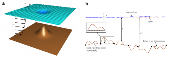
Figure 1: (a) Schematic of a unidirectional sub-critical flow showing that the free surface (exaggerated) dips down while flowing over a seamount. This permanent feature at the free surface is present along with transient features like surface gravity waves. (b) Medium/small-scale topographic features (of height $b$) present on the top of large-scale features. The free surface elevation $\eta$ and the ‘mean depth’ $H$ are calculated with respect to the the geoid, while the water depth $h$ is the distance between the free surface and the sea-bed. Between two successive black dots, the large-scale topography is nearly flat (see inset).

Attempts have also been made to reconstruct ocean bathymetry using the principles of fluid dynamics Vasan and Deconinck (2013). Vasan and Deconinck Vasan and Deconinck (2013) emphasize the ill-posed nature of this inverse problem, and show that bathymetry reconstruction is possible in idealized scenarios and under certain regimes, specifically the shallow water regime. They found that for bathymetry reconstruction, the surface elevation and its first two time derivatives as functions of the horizontal variable at several successive instances of time are needed. The practical feasibility of obtaining the input data, and hence the application of this method in real-world scenario is questionable.
  Here we propose a new inversion technique that reconstructs bottom topography with a uniform resolution and reasonably high accuracy from the free surface elevation and velocity field. Since both ocean surface elevation and velocity data can be obtained from satellite altimetry, our proposed technique can be directly implemented to reconstruct real ocean bathymetry.
  Large scale oceanic flows are in geostrophic and hydrostatic balance, which cause the free surface to tilt permanently (Vallis, 2017). Semi-permanent free surface tilts are also produced by wind-stress and flow over topography. In the latter case, the underlying principle can be explained using the theory of open-channel hydraulics; see Fig. 1(a). Oceanic circulation is strongly affected by its geometric shallowness. This significantly simplifies the governing equations of motion (vertical dynamics become negligible in comparison to the horizontal), yielding the celebrated shallow water equations (SWEs) (Vallis, 2017), which form the basis of open-channel hydraulics. In presence of planetary rotation and absence of viscous forces, the two-dimensional (2D) SWEs in Cartesian coordinates are given by

$$\frac{\partial h}{\partial t}+\ \frac{\partial(uh)}{\partial x}+\frac{\partial(vh)}{\partial y}=0,$$ (1)

$$\frac{\partial u}{\partial t}+u\frac{\partial u}{\partial x}+v\frac{\partial u}{\partial y}-fv=-g\frac{\partial\eta}{\partial x},$$ (2)

$$\frac{\partial v}{\partial t}+u\frac{\partial v}{\partial x}+v\frac{\partial v}{\partial y}+fu=-g\frac{\partial\eta}{\partial y}.$$ (3)

Here $h(x,y,t)$ is the water depth, $u(x,y,t)$ and $v(x,y,t)$ are respectively the $x$ (zonal) and $y$ (meridional) components of the horizontal velocity, $f$ is the Coriolis frequency ($f\equiv 2\Omega\sin\theta$, where $\Omega=7.2921\times 10^{-5}$ s^-1 is Earth’s rotation rate and $\theta$ is the latitude of interest), $g=9.81$ ms^-2 is the acceleration due to gravity, $\eta(x,y,t)=h(x,y,t)+b(x,y)-H$ is the free surface elevation, $H$ and $b$ respectively being the mean depth and the bottom topography; see Fig. 1(b).

For a steady, one-dimensional (1D) flow in the absence of rotation, Eqs. (1)-(3) can be highly simplified. These equations under linearization about the base velocity $U$ and the base height $H$ yield (Whitehead, 1998; Henderson, 1996; Chaudhry, 2007)

$$\frac{db}{dx}=\left(\frac{Fr^{2}-1}{Fr^{2}}\right)\frac{d\eta}{dx},$$ (4)

where $Fr\equiv U/\sqrt{gH}$ denotes the Froude number. For sub-critical flows $Fr<1$, hence the bottom slope $db/dx$ and the free surface slope $d\eta/dx$ have opposite signs. This mathematically justifies why flow over a bump produces a free surface dip. The concept of open-channel flows can be extended to oceans. Oceanic flows are usually highly sub-critical since $U\sim O(0.1-1)$ ms^-1, while $c\approx 200$ ms^-1 for an ocean with $H=4$ km. Hence one can expect a small depression at the ocean free surface right above a seamount.

Fourier transform of Eq. (4) relates the amplitude of the free surface dip, $\hat{\eta}$, to the topography amplitude, $\hat{b}$:

$$\hat{\eta}(k)=\left(\frac{Fr^{2}}{Fr^{2}-1}\right)\hat{b}(k),$$ (5)

where $k$ denotes the wavenumber and ‘hat’ denotes the transformed variable (signifying the amplitude corresponding to $k$). Since in oceans $Fr\sim 0.01$ – $0.001$, the free surface imprint of a topography $\hat{b}=100$ m will be $\sim 10-0.1$ mm. Modern altimeters have the ability to largely detect such small amplitude free surface anomalies(Smith and Sandwell, 2004).

Based on the fundamental theory of open-channel hydraulics we make two crucial observations: (i) whenever there is a quasi-steady open flow over a topography, the shape of the latter gets imprinted on the free surface, and (ii) the imprint is quasi-permanent, and can therefore be inverted to reconstruct the bottom topography.

As we have already shown, in an idealized, steady 1D flow, the bottom topography can be successfully reconstructed from the free surface elevation using Eq. (5). In a real ocean scenario, the free surface elevation contains transient features like surface waves along with the following major quasi-permanent features: (i) the tilt due to the geostrophic flow, $\eta_{g}$, (ii) tilt due to wind stress, $\eta_{s}$ and (iii) topography’s free surface imprint, $\eta_{b}$. For now we will assume that there are no wind-stresses, hence $\eta_{s}=0$. If the geostrophic velocity field $\bf{u_{g}}$ is known, $\eta_{g}$ can be computed as follows:

$$\nabla\eta_{g}=-\frac{f}{g}\mathbf{\hat{k}}\times\mathbf{u_{g}},$$ (6)

where $\bf{\hat{k}}$ is the unit-vector in the vertical direction. Following Vallis Vallis (2017), the non-dimensional form of Eqs. (2)–(3) can be written as:

$$Ro\left[\frac{\partial\hat{\mathbf{u}}}{\partial\hat{t}}+(\hat{\mathbf{u}}\cdot\nabla)\hat{\mathbf{u}}\right]+\hat{z}\times\hat{\mathbf{u}}=\frac{Ro}{{Fr}^{2}}\lambda\nabla\hat{\eta}.$$ (7)

Here, $Ro=U/{fL}$ is the Rossby number, $L$ is the horizontal length scale and $L/U$ is the advective timescale; $\lambda=\Delta\eta$/$H$, $h=H(1+\lambda\hat{\eta})-b$, $\hat{\eta}=\eta/\Delta\eta$, and $\Delta\eta$ is the scale of $\eta$. Variables with ‘hat’ denote the non-dimensional variables. Note that $Fr$ is independent of $L$ and is usually small in oceans ($Fr\approx 0.01$ – $0.001$). Since $Ro$ can change depending on $L$, we choose $Fr$ as the ‘small parameter’ and vary $Ro$.
When $L\approx 1000$ km, $Ro$ is a small number. The choice $Fr\sim Ro\sim\epsilon$, where $0<\epsilon\ll O(1)$ is a small parameter, leads to the balance between the Coriolis term and the RHS in Eq. (7), and for this we must have

$$\frac{Ro}{{Fr}^{2}}\lambda\sim O(1).$$

This is nothing but the geostrophic balance, i.e. Eq. (6). Since $\lambda\sim\epsilon$, we observe that

$$\Delta\eta_{g}\sim\epsilon H.$$

When $L\ll 100$ km, i.e. typical bathymetry scales we are interested in reconstructing, we find that $Ro\gtrsim O(1)$ (rotation plays a minor role). Hence the balance yields $\lambda\sim Fr^{2}\sim\epsilon^{2}$, which straightforwardly implies

$$\Delta\eta_{b}=\epsilon^{2}H.$$

Thus $\eta_{g}\gg\eta_{b}$, which means that the time average of the free surface elevation (by which transient features are removed) $\eta$ can be expressed as a two-term perturbation expansion

$$\langle\eta\rangle=\eta_{g}+\eta_{b},$$ (8)

where the angle brackets denote time averaging. Once $\eta_{g}$ is removed from the free surface by applying Eq. (6), the only free surface feature left that would be left is $\eta_{b}$.

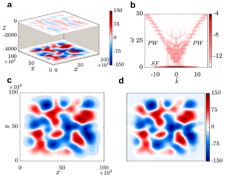
Figure 2: (a) Imprint of the bottom topography on the free surface for $Fr=0.001$. The free surface anomaly field (geostrophic effects removed) has been multiplied by $10^{4}$ to make it visible within the colorbar scale. (b) Wavenumber ($\tilde{k}$, in km^-1) – frequency ($\omega$, in s^-1) spectrum of the free surface anomaly. ‘PW’ denotes the dispersion relation of Poincar$\acute{\mathrm{e}}$ waves, while ‘SF’ denotes the same for the ‘stationary features’. The colors denote magnitude (in log scale) of the free surface anomaly spectra. (c) Actual topography, $b(x,y)$. (d) Topography reconstructed from the free surface data. For (a), (c) and (d), colors denote the height field (in m).

Time averaging of the shallow water mass conservation equation, i.e.  Eq. (1), and removal of $\eta_{g}$ from the free surface elevation yields

$$\frac{\partial}{\partial x}(b\bigl{\langle}u\bigr{\rangle})+\frac{\partial}{\partial y}(b\bigl{\langle}v\bigr{\rangle})=\frac{\partial}{\partial x}\bigl{\langle}(\eta_{b}+H)u\bigr{\rangle}+\frac{\partial}{\partial y}\bigl{\langle}(\eta_{b}+H)v\bigr{\rangle}.$$ (9)

After specifying appropriate boundary conditions for $b$ (zero at the boundaries), the above equation is solved using finite difference scheme to reconstruct $b$ entirely from the free surface data ($u$, $v$ and $\eta_{b}$). Although $H$ is not a surface variable, it is already known a-priori from the coarse-resolution data. Since the free surface velocities and elevation can be obtained from satellite altimetry data,  Eq. (9) can be directly used to reconstruct ocean bathymetry.

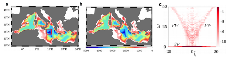
Figure 3: Mediterranean sea bathymetry reconstruction using MITgcm. (a) Actual bathymetry from GEBCO, and (b) reconstructed bathymetry. The color contours represent depth $h$ (in m) from the free surface. (c) Wavenumber ($\tilde{k}$, in km^-1) – frequency ($\omega$, in s^-1) spectrum of the free surface anomaly of a part of the Mediterranean sea (marked by red-color box in (a)). The colors denote magnitude (in log scale) of the free surface anomaly spectra.

First we consider a simplified toy ocean model that is governed by the 2D SWEs with planetary rotation, i.e.  Eqs. (1)-(3). The mean topography is a flat horizontal surface on which Gaussian mountains and valleys of random amplitudes are added. The initial velocity field is under geostrophic and hydrostatic balance. We prescribe the initial height field as $H_{0}=H+\eta_{g}$, where the mean depth $H=4$ km, and the geostrophic tilt is

$$\eta_{g}=0.1\tanh(\mathcal{Y})+0.03\operatorname{sech}^{2}(\mathcal{Y})\sin\Big{(}\frac{2\pi x}{L_{x}}\Big{)},$$

where $\mathcal{Y}\equiv(0.5L_{y}-y)/(2L_{y})$. For numerical computation, a doubly-periodic horizontal domain of $L_{x}\times L_{y}=10^{5}$ m $\times 10^{5}$ m is assumed. The grid-size is $10^{3}$ m in both $x$ and $y$ directions, and time-step size is $1$ s. The numerical model uses second order central differencing for spatial and fourth order Runge-Kutta for temporal discretization, and is integrated for 10 days, by which a quasi-steady state is reached. On time-averaging the free surface elevation using Eq. (8), we obtain the quasi-stationary features. The geostrophy induced tilt $\eta_{g}$ is removed using Eq. (6). The remaining feature contains the bathymetry induced tilt $\eta_{b}$. This $\eta_{b}$, also shown in Fig. 2(a) (in Fig. 2(b), it is shown as ‘SF’ in the Fourier space), is inverted to reconstruct the bottom topography using Eq. (9). The comparison between the actual and the reconstructed topography is shown in Figs. 2(c)–2(d), the $L_{2}$-norm error is found to be 0.35%.

The problem can also be approached by performing Fourier-transform on the free surface anomaly data to obtain the wavenumber ($\tilde{k}$) – frequency ($\omega$) spectrum ($\tilde{k}=\sqrt{k^{2}+l^{2}}$ is the magnitude of the horizontal wavenumber vector ($k,l$)), see Fig. 2(b). The spectrum shows both positively and negatively traveling Poincar$\acute{\mathrm{e}}$ waves (indicated by ‘PW’), whose dispersion relation is

$$\omega^{2}=f^{2}+{gH}{\tilde{k}}^{2}.$$ (10)

The stationary feature or ‘SF’, located along $\omega\approx 0$, has the highest magnitude. Inverse Fourier transform of SF yields $\langle\eta\rangle$, and thus $\eta_{b}$, from which the bottom topography can be reconstructed using Eq. (9). An important point worth noting is that knowing $H$ a-priori is not mandatory; the ($\omega$, $\tilde{k}$) values in Fig. 2(b) can be substituted in the dispersion relation Eq. (10) to obtain $H$.

Based on the fundamental understanding of the 2D shallow water system, we have pursued bathymetry reconstruction of a more complicated, semi-realistic system. We have performed this particular exercise keeping in mind that in real ocean scenario, the density changes are significantly small (approximately $\lesssim 2\%$ from a reference value). Furthermore, the large-scale motions are approximately in hydrostatic balance, hence the dynamics can be well explained using a simplified one-layer shallow water model (Gill, 1982). In this regard we solve the 3D Navier-Stokes equations along with the evolution equations of temperature and salinity using MITgcm. The latter is an open-source code that solves the following non-linear, non-hydrostatic, primitive equations (under Boussinesq approximation) in spherical coordinate system using the finite volume method(Marshall et al., 1997).

We intend to simulate the Mediterranean sea, the horizontal domain extent of which is $8\degree$W - $36\degree$E in longitude and $30.5\degree$N - $46\degree$N in latitude. We consider a grid resolution of $\sim$ $0.1\degree\times 0.1\degree$, which results in $435\times 140$ grid points. In the vertical (radial) direction we consider $60$ non-uniformly spaced grid points, which varies from $1$ m at the free surface to a maximum value of $200$ m in the deeper regions. The horizontal viscosity and diffusivity terms are modeled using bi-harmonic formulation with $1.5\times 10^{10}$ m⁴/s as both viscosity and diffusivity coefficients (Calafat et al., 2012). Following Wunsch and FerrariWunsch and Ferrari (2004), the vertical eddy-diffusivity for temperature and salinity are considered to be $10^{-5}$ m²s^-1. Likewise, the vertical viscosity coefficient is assumed to be $1.5\times 10^{-4}$ m²s^-1, following Calafat et al. Calafat et al. (2012). The lateral and bottom boundaries satisfy no-slip and impenetrability conditions. The numerical model incorporates implicit free surface with partial-step topography formulation (Adcroft, Hill, and Marshall, 1997).

The bottom topography of the Mediterranean sea (see Fig. 3(a)) is taken from The General Bathymetric Chart of the Oceans’ (GEBCO) gridded bathymetric datasets (Weatherall et al., 2015). The currently available resolution, based on ship-based survey and satellite altimetry combined, is $30$ arc-seconds. For our numerical simulation purposes, the topography data has been interpolated to our grid resolution.

The numerical model has been initialized with 3D temperature, salinity, horizontal velocity (both zonal and meridional components), and free surface elevation data from Nucleus for European Modelling of the Ocean (NEMO) re-analysis data obtained from Copernicus Marine Service Products (von Schuckmann et al., 2016). The input variables, taken on 12^th December 2017, are time-averaged (over that given day), and then interpolated to the grid resolution. The model has been integrated for $30$ days with a constant time-step of $100$ s so as to reach a quasi-steady state.

For calculating $\eta_{g}$, the free surface velocity over the last $7$-days of the simulation are taken and subsequently time-averaged, yielding the geostrophic velocity. At boundaries we set $\eta_{g}=0$ and solve Eq. (6). The geostrophic velocity satisfies the horizontal divergence-free condition, hence contains no information about the the bottom topography. Topography information is contained in the ageostrophic velocity part.

In order to do the reconstruction, we have averaged the free surface velocity field over $12$ hours. This averaging time has been judiciously chosen – not too long so that the flow is geostrophic, and not too short so that the surface elevation gets affected by surface waves. For $H$ we have taken a resolution of $\sim 0.5\degree$ in both latitude and longitude directions so as to mimic the large scale topographic structure. For the reconstruction we solve the spherical coordinate version of Eq. (9). For ease of understanding, the solution algorithm is given below:

Algorithm 1 Procedure for finding $b$

1:procedure inverse bathymetry

2:     input: $H$, $u$ and $v$ at the free-surface ($\eta$)

3:     process:

4:     Step 1: Find the geostrophic flow induced tilt – take 7 days time average of $u$ and $v$ to get the geostrophic flow and use Eq. (6) to find $\eta_{g}$.

5:     Step 2: Find $\eta_{b}$ – take 12 hours time average of $\eta$ and subtract $\eta_{g}$ to get $\eta_{b}$ (use Eq. (8)).

6:     Step 3: Solve the spherical coordinate version of Eq. (9) to get $b$.

7:end procedure

The reconstructed bottom topography, shown in Fig. 3(b), is $\approx 97.6\%$ accurate. We emphasize here that the spherical coordinate version of Eq. (9), used for bathymetry reconstruction, is a diagnostic equation since we have not imposed shallow water approximation anywhere in MITgcm. Hence the large-scale 2D flow is primarily important for bathymetry reconstruction, additional effects of density stratification and three-dimensionality are insignificant.

As mentioned earlier, Fourier transform of the free surface provides an alternative technique to bathymetry reconstruction. Fig. 3(c) shows the Fourier transform of the free-surface anomaly (after removing the geostrophic flow induced tilt) of the boxed region (red-colored line) marked in the Mediterranean sea (see Fig. 3(a)). The free surface contains stationary features (which contains the information about the underlying bathymetry), marked by ‘SF’, and wave-like signatures, marked by ‘PW’. By inverting SF, one can reconstruct the bathymetry of the boxed region.

Finally we attempt to reconstruct ocean bathymetry completely from re-analysis data. We have first chosen Red sea in this regard, the necessary data for which is obtained from HYCOM (Hybrid Coordinates Ocean Model) based NOAA Global forecast system (Chassignet et al., 2007). It provides $3$-hourly global ocean data with a horizontal resolution of $1/12\degree$ for $40$ vertical depth levels. The model uses ETOPO5 topography data of $1/12\degree$ resolution (NOAA, 1988). We have taken $5$ datasets of 2017, each of $7$-day length: $5^{\mathrm{th}}-11^{\mathrm{th}}$ March, $12^{\mathrm{th}}-18^{\mathrm{th}}$ April, $8^{\mathrm{th}}-14^{\mathrm{th}}$ May, $15^{\mathrm{th}}-21^{\mathrm{st}}$ June and $9^{\mathrm{th}}-15^{\mathrm{th}}$ July. Corresponding to each dataset, first the geostrophic velocity is calculated by performing a $7$-day time-average and calculate $\eta_{g}$ using Eq. (6). In oceans, wind-stress $\bm{\tau}$ is always present, and is obtained from the wind velocity data Gill (1982):

$$\centering\bm{\tau}=\rho_{a}C_{d}\mathbf{u}_{a}|\mathbf{u}_{a}|,\@add@centering$$ (11)

where $\rho_{a}=1.2$ kg/m³ is the density of air, $C_{d}$ is the drag coefficient and $\mathbf{u}_{a}$ is the wind velocity. The value of $C_{d}$ is calculated for every $6$ hours as a function of wind velocities and temperature differences between air ($T_{a}$) and sea surface ($T_{s}$) using the following polynomial formula Hellerman and Rosenstein (1983):

$$C_{d}=\alpha_{1}+\alpha_{2}|\mathbf{u}_{a}|+\alpha_{3}(T_{a}-T_{s})+\alpha_{4}|\mathbf{u}_{a}|^{2}\\ +\alpha_{5}(T_{a}-T_{s})^{2}+\alpha_{6}|\mathbf{u}_{a}|(T_{a}-T_{s}),$$

where $\alpha$ with subscripts $1,2,...6$ are constants, the values of which are taken from Eq. $(11)$ of Hellerman and Rosenstein Hellerman and Rosenstein (1983). $T_{a}$ is taken at $2$ m above the sea level, and is obtained from the ECMWF ERA-Interim re-analysis data on the same dates of interest. Likewise, $T_{s}$ is obtained from NEMO-MED reanalysis data of Copernicus Marine Service Products. Wind stress causes quasi-stationary free surface elevation $\eta_{s}$, which is given byJanzen and Wong (2002):

$$\nabla\eta_{s}=\frac{\bm{\tau}}{g\rho_{w}H},$$ (12)

where $\rho_{w}$ is the density of water, and it is assumed that the wind-stress is small and therefore does not affect the inertial acceleration. Depending on whether we are using Cartesian or spherical coordinate system, the $\nabla$ operator is chosen accordingly.
In reality, wind-stress can occasionally become large (e.g. storm events), making the wind-stress induced tilt calculation invalid. For this reason, the datasets are carefully selected such that low wind velocity is ensured. The time-averaged free surface elevation is now given by

$$\langle\eta\rangle=\eta_{g}+\eta_{s}+\eta_{b},$$ (13)

and, although it is more complicated than Eq. (8), still we have the recipe of removing $\eta_{s}$ following Eq. (12). After removing both $\eta_{g}$ and $\eta_{s}$, only free surface feature left is $\eta_{b}$. At last, the bathymetry is reconstructed using the spherical coordinate version of Eq. (9), in which the free surface velocity and elevation data are $12$-hours time-averaged. The resolution of the mean depth $H$ is taken to be $6$ times coarser ($1/2\degree$). For each dataset we obtain an inverted bathymetry map, the final map is the average of the five datasets. The original and the reconstructed bathymetry are compared in Figs. 4(a)-4(b); the average reconstruction error is $12.51\%$.
A similar technique can be followed in reconstructing any other bathymetry. For example, we reconstruct Mediterranean sea bathymetry using the following $5$ datasets: $1^{\mathrm{st}}-7^{\mathrm{th}}$ May, $12^{\mathrm{th}}-18^{\mathrm{th}}$ June, $7^{\mathrm{th}}-13^{\mathrm{th}}$ July, $20^{\mathrm{th}}-26^{\mathrm{th}}$ August and $15^{\mathrm{th}}-21^{\mathrm{st}}$ September. The actual and reconstructed bathymetries are shown in Figs. 4(c)-4(d), the average reconstruction error is $12.68\%$.

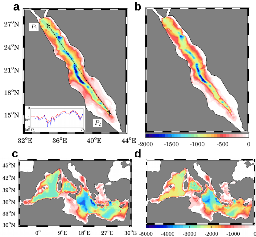
Figure 4: Bathymetry reconstruction from real data. (a) Original and (b) reconstructed Red sea bathymetry. The inset of (a) shows a comparison between the original (blue line) and reconstructed (red line) topography along the line $P_{1}P_{2}$ ($14.31\%$ error). (c) Original and (d) reconstructed Mediterranean sea bathymetry. The color contours in (a-d) represent depth $h$ (in m) from the free surface.

In conclusion, we have shown that for shallow, free surface flows, the geometric information of the underlying topography remains embedded in the free surface. Based on the shallow water mass conservation equation, we have proposed a simple inversion technique that successfully reconstructs the bottom topography from the free surface elevation and velocity field. We have applied this technique to (i) a toy ocean model, (ii) global circulation model (MITgcm) initialized by re-analysis data, and finally, (iii) purely re-analysis data. For the MITgcm case, we reconstruct Mediterranean sea bathymetry of $0.1\degree$ resolution with $97.6$% accuracy. For pure re-analysis data, both Red and Mediterranean sea bathymetries of $1/12\degree$ resolution are reconstructed with $\approx 90$% accuracy.

In conjunction with ship echo-soundings, our reconstruction technique may provide a highly accurate global bathymetry map in the future. The problem remains to be tested on data fully obtained from satellite altimetry. At present, satellites do not provide very reliable information in the horizontal-scale of $\lesssim 100$ km. In near future, the Surface Water Ocean Topography (SWOT) satellite mission will revolutionize the field by providing information at unprecedented scales of $15-25$ km, which is of an order of magnitude higher resolution than that of current satellites Gaultier, Ubelmann, and Fu (2016). Our technique will be specifically useful in obtaining accurate bathymetry maps of the shallow coastal regions, where the estimated reconstruction time by ship-based surveying is 750 ship-years.

This work has been partially supported by the following grants: IITK/ME/2014338, STC/ME/2016176 and ECR/2016/001493.

References

- Smith and Sandwell (1997) W. H. Smith and D. T. Sandwell, Science 277, 1956 (1997).
- Wessel (1997) P. Wessel, Science 277, 802 (1997).
- Mofjeld et al. (2004) H. O. Mofjeld, C. M. Symons, P. Lonsdale, F. I. González, and V. V. Titov, Oceanography 17, 38 (2004).
- Fairhead, Green, and Odegard (2001) J. D. Fairhead, C. M. Green, and M. E. Odegard, The Leading Edge 20, 873 (2001).
- Munk and Wunsch (1998) W. Munk and C. Wunsch, Deep Sea Res. Part 1 Oceanogr. Res. Pap. 45, 1977 (1998).
- Nicholls and Taber (2009) D. P. Nicholls and M. Taber, Eur. J. Mech. B Fluids. 28, 224 (2009).
- Becker et al. (2009) J. Becker, D. Sandwell, W. Smith, J. Braud, B. Binder, J. Depner, D. Fabre, J. Factor, S. Ingalls, S. Kim, et al., Mar Geod. 32, 355 (2009).
- Smith and Sandwell (2004) W. H. Smith and D. T. Sandwell, Oceanography 17, 8 (2004).
- Smith and Sandwell (1994) W. H. Smith and D. T. Sandwell, J. Geophys. Res.: Solid Earth 99, 21803 (1994).
- Vasan and Deconinck (2013) V. Vasan and B. Deconinck, J. Fluid Mech. 714, 562 (2013).
- Vallis (2017) G. K. Vallis, Atmospheric and oceanic fluid dynamics (Cambridge University Press, 2017).
- Whitehead (1998) J. Whitehead, Rev. Geophys. 36, 423 (1998).
- Henderson (1996) F. M. Henderson, Open channel flow (Macmillan, 1996).
- Chaudhry (2007) M. H. Chaudhry, Open-channel flow (Springer Science & Business Media, 2007).
- Gill (1982) A. E. Gill, Atmosphere–ocean dynamics, (Academic Press, 1982).
- Marshall et al. (1997) J. Marshall, A. Adcroft, C. Hill, L. Perelman, and C. Heisey, J. Geophys. Res. 102, 5753 (1997).
- Calafat et al. (2012) F. M. Calafat, G. Jordà, M. Marcos, and D. Gomis, J. Geophys. Res.: Oceans 117(C02009), 1 (2012).
- Wunsch and Ferrari (2004) C. Wunsch and R. Ferrari, Ann. Rev. Fluid Mech. 36, 281 (2004).
- Adcroft, Hill, and Marshall (1997) A. Adcroft, C. Hill, and J. Marshall, Month. Weather Rev. 125, 2293 (1997).
- Weatherall et al. (2015) P. Weatherall, K. Marks, M. Jakobsson, T. Schmitt, S. Tani, J. E. Arndt, M. Rovere, D. Chayes, V. Ferrini, and R. Wigley, Earth and Space Science 2, 331 (2015).
- von Schuckmann et al. (2016) K. von Schuckmann et al., J. Oper. Oceanogr. 9, s235 (2016).
- Chassignet et al. (2007) E. P. Chassignet, H. E. Hurlburt, O. M. Smedstad, G. R. Halliwell, P. J. Hogan, A. J. Wallcraft, R. Baraille, and R. Bleck, Journal of Marine Systems 65, 60 (2007).
- NOAA (1988) NOAA, NOAA/National Geophysical Data Center, Boulder, CO. (1988).
- Hellerman and Rosenstein (1983) S. Hellerman and M. Rosenstein, J. Phys. Oceanogr. 13, 1093 (1983).
- Janzen and Wong (2002) C. D. Janzen and K.-C. Wong, J. Geophys. Res.: Oceans 107 (2002).
- Gaultier, Ubelmann, and Fu (2016) L. Gaultier, C. Ubelmann, and L.-L. Fu, J. Atmospheric Ocean. Technol. 33, 119 (2016).