Black-hole Spectroscopy by Making Full Use of Gravitational-Wave Modeling

Abstract

The Kerr nature of a compact-object–coalescence remnant can be unveiled by observing multiple quasi-normal modes in the post-merger signal. Current methods to achieve this goal rely on matching the data with a superposition of exponentially damped sinusoids with amplitudes fitted to numerical-relativity (NR) simulations of binary black-hole mergers. These models presume the ability to correctly estimate the time at which the gravitational-wave signal starts to be dominated by the quasi-normal modes of a perturbed black hole. Here we show that this difficulty can be overcome by using multipolar inspiral-merger-ringdown waveforms, calibrated to NR simulations, as already developed within the effective-one-body formalism (EOBNR). We build a parameterized (nonspinning) EOBNR waveform model in which the quasi-normal mode complex frequencies are free parameters (pEOBNR), and use Bayesian analysis to study its effectiveness in measuring quasi-normal modes in GW150914, and in synthetic gravitational-wave signals of binary black holes injected in Gaussian noise. We find that using the pEOBNR model gives, in general, stronger constraints compared to the ones obtained when using a sum of damped sinusoids and using Bayesian model selection, we also show that the pEOBNR model can successfully be employed to find evidence for deviations from General Relativity in the ringdown signal. Since the pEOBNR model properly includes time and phase shifts among quasi-normal modes, it is also well suited to consistently combine information from several observations — e.g., we find on the order of $\sim 30$ GW150914-like binary black-hole events would be needed for Advanced LIGO and Virgo at design sensitivity to measure the fundamental frequencies of both the $(2,2)$ and $(3,3)$ modes, and the decay time of the $(2,2)$ mode with an accuracy of $\lesssim 5\%$ at the $2\mbox{-}\sigma$ level, thus allowing to test the black hole’s no-hair conjecture.

I Introduction

Up to now, all the observed gravitational waves (GWs) from the coalescence of compact objects by Advanced LIGO and Virgo Abbott et al. (2016a, b, 2017a, 2017b, 2017c) are entirely consistent with the expected gravitational radiation emitted during the inspiral, merger and ringdown stages of a binary black hole (BBH), as predicted by Einstein theory of General Relativity (GR) Abbott et al. (2016c, d) (however, note that GW170817 Abbott et al. (2017d, 2018) was most likely a binary neutron star event due to its electromagnetic counterpart). After merger, GR predicts that the remnant black hole (BH) is described by the Kerr metric Kerr (1963), the unique stationary, axisymmetric and asymptotically flat BH solution of the Einstein field equations in vacuum (astrophysical BHs are thought to be electrically neutral). As detectors with improved sensitivity and longer observation times come online, the signal-to-noise ratio (SNR) and number of events will increase, and more stringent gravitational tests could put GR at stake Will (2014); Berti et al. (2015), and/or reveal the existence of exotic astrophysical compact objects Mazur and Mottola (2004); Visser and Wiltshire (2004); Liebling and Palenzuela (2012) in our Universe.

Consistent with theoretical predictions, the GW signals of the five BBHs observed so far by Advanced LIGO, GW150914, GW151226, GW170104, GW170608 and GW170814, chirp from the inspiral stage, where the orbital frequency increases as the two objects come closer and closer, up to merger, where the GW luminosity reaches a peak and non-perturbative GR effects dominate. After the merger, the waveform settles to a linear superposition of exponentially damped sinusoidal oscillations (ringdown) or quasi-normal modes (QNMs), described by a discrete set of complex frequencies which are uniquely determined by the nature of the remnant BH and are independent on how the BH was formed. That BHs, when formed and/or perturbed, emit GWs described by a very specific set of QNMs was discovered in the early 70s Vishveshwara (1970); Press (1971); Chandrasekhar and Detweiler (1975). In vacuum, the no-hair theorems Israel (1967); Carter (1971); Hawking (1972); Robinson (1975) imply that in GR the BH’s QNMs depend only on the BH’s mass $M_{\rm BH}$ and angular momentum (or spin) $J_{\rm BH}$, and therefore testing this hypothesis requires the identification of at least two QNMs in the ringdown waveform Dreyer et al. (2004); Berti et al. (2006); Gossan et al. (2012); Meidam et al. (2014); Yang et al. (2017); Da Silva Costa et al. (2017)  .

The idea of employing spectroscopy of the ringdown stage of compact-object binary mergers to prove that a BH has been observed (or better rule out/constrain theories alternative to GR or other compact objects rather than BHs) and test the no-hair hypothesis in GR, was first examined in Ref. Dreyer et al. (2004). Later, Ref. Berti et al. (2006) carried out a comprehensive study aimed at quantifying the accuracy with which the QNM (complex) frequencies can be measured for GW sources observable by the laser-interferometer space-based antenna (LISA), and applied statistical criteria to estimate the resolvability of different modes. The latter was also used in subsequent publications (e.g., see Refs. Berti et al. (2007a); Bhagwat et al. (2016); Berti et al. (2016); Maselli et al. (2017)), which focused also on future GW detectors on the ground. An important step in understanding the feasibility of the BH–spectroscopy program came with Refs. Gossan et al. (2012); Meidam et al. (2014), where the authors applied Bayesian techniques for the first time, employed parameterized models for the ringdown signals and advocated for the use of multiple events to get stronger tests of the GR no-hair conjecture. More recently, Ref. Yang et al. (2017) proposed a strategy to increase the accuracy of observing a given QNM by constructively summing the ringdown signal from multiple events, after appropriately applying a rescale and time shift such that the QNM in all signals has the same frequency and phase. The same idea was proposed in Ref. Da Silva Costa et al. (2017) although only implemented for the least-damped QNM. We stress, that this recent idea to extract subdominant modes relies on using the measured BBH parameters (i.e., masses and spins), and importantly on knowing in advance the relative phases and amplitudes of the excited QNMs.

In previous analyses of the BH–spectroscopy program, all studies were conducted employing for the ringdown signal a superposition of exponentially damped sinusoids with either free amplitudes and phases Berti et al. (2006); Maselli et al. (2017); Cabero et al. (2017) or with amplitudes fitted to numerical-relativity (NR) simulations Berti et al. (2007a); Gossan et al. (2012); Meidam et al. (2014). Here, by contrast, we make full use of GW modeling from BBH coalescences and employ inspiral-merger-ringdown (IMR) waveforms as developed within the effective-one-body formalism Buonanno and Damour (1999, 2000), augmented by NR simulations Pan et al. (2011) (EOBNR waveforms, for short ). There are two main advantages in doing so. First, EOBNR waveforms include, by construction, the phase difference between different QNMs, tuned to NR simulations, thus avoiding to apply sophisticated techniques to enforce such a coherence a posteriori (i.e., after the observation Yang et al. (2017); Da Silva Costa et al. (2017)). Second, there is no need to define an a priori unknown time at which the QNMs start to dominate the post-merger signal (or select a few arbitrary values, as was done for GW150914 Abbott et al. (2016c)), because this time is automatically taken into account when building EOBNR waveforms, so that they match NR waveforms with high precision. As we shall see, the apparent limit in the accuracy of extracting QNM frequencies, as recently advocated in Ref. Thrane et al. (2017), does not hold when employing IMR waveforms.

The rest of this paper is organized as follows. We first introduce our IMR waveform model with free QNM complex frequencies in Sec. II, and discuss how this model can be used to measure the ringdown frequencies and damping time of a BBH-coalescence remnant. In Sec. III we present the statistical method that we employ to measure the QNM complex frequencies, and test the IMR model against the GW event GW150914 and NR waveforms. Section IV studies two different approaches to measure deviations from GR using the IMR waveform model. We first perform a Bayesian model selection study to show that the IMR model is able to find evidence for deviations from GR in the ringdown. Then, we give some prospects, using Advanced LIGO and Virgo noise curves at design sensitivity, on how strongly the model can constrain deviations from GR by combining several detections. Finally, we summarize and discuss future improvements in Sec. V.

II Full gravitational-wave signal to extract quasi-normal modes

We use the IMR waveforms developed within the EOB formalism, which provides a faithful and physical, semi-analytic description of the full coalescence process, and it can be made highly accurate by including information from NR simulations. In particular, here we employ the multipolar waveform model for nonspinning BBHs calibrated to NR simulations in Ref. Pan et al. (2011) (henceforth, EOBNR for short). A GW emitted from a binary into a given sky direction $(\theta,\phi)$ can be written as $h_{+}(\theta,\phi;t)-ih_{\times}(\theta,\phi;t)=\sum_{\ell,m}{}_{-\!2}Y_{\ell m}(\theta,\phi)\,h_{\ell m}(t)$, where ${}_{-\!2}Y_{\ell m}(\theta,\phi)$ are the $-2$ spin-weighted spherical harmonics. Our EOBNR model includes the $(\ell,|m|)=(2,1)$, $(3,3)$, $(4,4)$, and $(5,5)$ modes besides the dominant $(2,2)$ mode.

More specifically, for each $(\ell,m)$, the merger-ringdown EOBNR modes read

$$h_{\ell m}^{\mathrm{merger-RD}}(t)=\sum_{n=0}^{N-1}A_{\ell mn}\,e^{-i\sigma_{\ell mn}(t-t_{\mathrm{match}}^{\ell m})}\quad t\geq t_{\rm match}^{\ell m}\,,$$ (1)

where $n$ is the QNM overtone number, $N$ is the number of overtones included in the EOBNR model (e.g., $N=8$ in Ref. Pan et al. (2011) ), and $A_{\ell mn}$ are complex amplitudes determined by the procedure that matches the merger-ringdown waveform to the inspiral-plunge EOBNR waveform $h_{\ell m}^{\mathrm{inspiral-plunge}}(t)$. Such a procedure guarantees differentiability at the matching point $t_{\mathrm{match}}^{\ell m}$. The quantity $\sigma_{\ell mn}=\omega_{\ell mn}-i/\tau_{\ell mn}$, where the oscillation frequencies $\omega_{\ell mn}>0$ and the decay times $\tau_{\ell mn}>0$, are numbers associated with each QNM. It was found in Refs. Barausse et al. (2012); Pan et al. (2011), that in the test-particle limit and comparable-mass case, the different modes can peak at different times, depending on mass ratio and spin values. We stress that the multipolar EOBNR model adopted here does reproduce this important feature by including appropriate time shifts between the modes ($\Delta^{\ell m}_{\rm match}$) in the matching procedure (for details see Fig. 1 and Sec. IIB in Ref. Pan et al. (2011)). Through this work we will use the same time shifts, $\Delta^{\ell m}_{\rm match}$, obtained in Ref. Pan et al. (2011). Finally, the inspiral-(plunge-)merger-ringdown EOBNR waveform reads $h_{\ell m}(t)=h_{\ell m}^{\mathrm{insp-plunge}}\,\theta(t_{\mathrm{match}}^{\ell m}-t)+h_{\ell m}^{\mathrm{merger-RD}}\,\theta(t-t_{\mathrm{match}}^{\ell m})$, where $\theta(t)$ is the Heaviside step function.

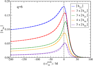
Figure 1: Comparison between modes’ amplitudes of the EOBNR model Pan et al. (2011) used here (dashed lines) and the NR waveform (solid lines) for a BBH simulation with mass ratio $q=6$ produced by the SXS collaboration Mroue et al. (2013). In the horizontal axis the time origin is chosen such that it corresponds to the peak of the $(2,2)$ mode.

In Ref. Pan et al. (2011), the complex frequencies $\sigma_{\ell m}$ were expressed in terms of the final BH mass and spin Berti et al. (2006), and the latter were related to the BBH’s component masses and spins through an NR–fitting-formula Pan et al. (2011) computed in GR. For concreteness, in Fig. 1 we show an example where we compare the amplitude of the different modes available in the EOBNR waveform, for a BBH with mass ratio $q=6$, against the waveform obtained from a NR simulation . Importantly, the model includes time shifts between the peak of each mode and agrees very well with NR, even for $\ell>2$-modes.

Here, to measure the ringdown frequencies and damping times of different QNMs, we build a parameterized EOBNR model by relaxing the assumption that the ringdown signal is fixed by the NR–fitting-formula in Ref. Pan et al. (2011), and instead promote the QNM (complex) frequencies to be free parameters (henceforth, pEOBNR model). In the specific applications of this paper, we will only allow $\sigma_{220}$ and $\sigma_{330}$ to vary freely, while all the other mode frequencies present in the merger-ringdown waveform coincide to the GR values. We emphasize that $\sigma_{220}$ and $\sigma_{330}$ varying freely implies that the EOBNR waveform at merger (i.e., close to the peak and at $t_{\mathrm{match}}^{\ell m}$), does not necessarily coincide with the GR prediction, since the matching procedure changes the shape of the waveform for $t>t_{\mathrm{match}}^{\ell m}$ for $(\ell,m)=(2,2)$ and $(3,3)$. Lastly, for $t<t_{\rm match}^{\ell m}$, our EOBNR waveform modes agree with the inspiral-plunge modes $h_{\ell m}^{\mathrm{inspiral-plunge}}(t)$ computed in GR. In the future, as the EOB formalism is extended to modified theories of GR Julié and Deruelle (2017); Julié (2018), we will include non-GR inspiral-plunge modes and other possible variations around merger.

In the following, we contrast the results obtained with the pEOBNR model, with a waveform model that consists of solely a superposition of damped sinusoids, whose (complex) frequencies are free parameters Dreyer et al. (2004); Berti et al. (2006). This has been the most common ringdown model used in the literature to test the no-hair conjecture and/or extract multiple QNMs. After the NR breakthrough in 2005, the relative amplitudes and phases of the QNMs in these models have been constrained using fits from NR simulations of BBHs Kamaretsos et al. (2012); Gossan et al. (2012); London et al. (2014); London (2018). More explicitly, the ringdown model that we employ is ($t\geq 0$)

$$h^{\rm RD}_{+}(\theta,\phi;t)=\sum_{\ell,m>0}A_{\ell|m|}\,e^{-t/\tau_{\ell m}}\,Y^{\ell m}_{+}(\theta)\cos(\omega_{\ell m}t-\phi_{\ell m})\,,$$ (2)

$$h^{\rm RD}_{\times}(\theta,\phi;t)=-\sum_{\ell,m>0}A_{\ell|m|}\,e^{-t/\tau_{\ell m}}\,Y^{\ell m}_{\times}(\theta)\sin(\omega_{\ell m}t-\phi_{\ell m}),$$ (3)

where $Y_{+}^{lm}\equiv{}_{-2}Y^{lm}+(-1)^{l}~{}_{-2}Y^{l-m}$ and $Y_{\times}^{lm}\equiv{}_{-2}Y^{lm}-(-1)^{l}~{}_{-2}Y^{l-m}$, and $h_{+}=h_{\times}=0,$ for $t<0$, $t=0$ being the starting time of the ringdown signal. Since we focus on nonspinning BBHs, we use for the relative modes’ amplitudes the NR-fits in Ref. Gossan et al. (2012), so that the only free parameters are the mode frequencies $\omega_{\ell m}$, damping times $\tau_{\ell m}$, the phases $\phi_{\ell m}$, the BBH mass ratio $q$ and an overall amplitude factor (see Eqs. (5)–(8) in Ref. Gossan et al. (2012)). One crucial difference of this ringdown model from the pEOBNR model discussed above, is that the former assumes that all modes start at the same time, and this is not observed in NR simulations of BBHs (see Fig. 1 and Ref. Pan et al. (2011)). Furthermore, the pEOBNR model also includes overtones beyond $n=0$, which can be excited around merger, as also observed in NR simulations Buonanno et al. (2007); Berti et al. (2007b).

An important difficulty to overcome when using a damped sinusoid model is the need to define a specific starting time at which the GW signal is well described by a sum of QNMs. Since the arrival time of the signal in the different detectors is a function of the sky position, to correctly define the time at which the ringdown starts in all detectors, one not only needs to know the geocentric time at coalescence but also the sky position of the signal Cabero et al. (2017). For a real event these parameters are a priori unknown and must be obtained from a previous analysis done with an IMR waveform. In addition to this difficulty, to avoid biases and accurately recover the ringdown parameters for an IMR signal, we also find it necessary to zero out the synthetic GW signals injected in Gaussian noise prior to the starting time of the damped sinusoid model. This behavior was already pointed out in Ref. Cabero et al. (2017), and is related to matching a model with a cutoff in the time domain to a signal that includes all the IMR information. These technical difficulties can be completely avoided by using an IMR model, and therefore provide an additional motivation for this work.

In summary, focusing on nonspinning BBHs with component masses $m_{1}$ and $m_{2}$, we consider two different waveform models: (i) the pEOBNR waveform built from Ref. Pan et al. (2011) with free parameters $\bm{\vartheta}_{\rm GR}=\{M_{c},q,D_{L},\alpha,\delta,\psi,\theta,t_{c},\phi_{c}\}$, where $M_{c}=M\nu^{3/2}$ is the (redshifted) chirp mass, with $\nu=m_{1}m_{2}/(m_{1}+m_{2})^{2}$ and $M$ the (redshifted) total mass, $q=m_{1}/m_{2}>1$ is the mass ratio, $D_{L}$ is the luminosity distance, $\theta$ is the inclination angle of the binary, $\alpha$, $\delta$ and $\psi$ are the right ascension, declination and polarization angles, respectively, and $t_{c}$ and $\phi_{c}$ are the (geocentric) time and phase at coalescence, supplemented with free complex QNM frequencies for the (220) and (330) modes $\bm{\vartheta}=\bm{\vartheta}_{\rm GR}\cup\{\omega_{220},\tau_{220},\omega_{330},\tau_{330}\}$; and (ii) the damped sinusoid model given by Eqs. (2) and (3). In this work we either use only one damped sinusoid, or use a two-damped sinusoid model with relative amplitudes for the (220) and (330) modes fitted to NR as given in Ref. Gossan et al. (2012), neglecting all the other modes. Therefore for the two-damped sinusoid model the free parameters are $\bm{\vartheta}_{\rm RD}=\{\omega_{220},\omega_{330},\tau_{220},\phi_{220},\tau_{330},\phi_{330},A,q\}$, with $A$ an overall amplitude, that can be related to the BH final mass and the luminosity distance, while for the single damped sinusoid model, the free parameters are simply $\bm{\vartheta}_{\rm RD}=\{\omega_{220},\tau_{220},\phi_{220},A\}$. We note that for both sinusoid models we fix the sky location $\{\alpha,\delta\}$ and geocentric time at coalescence $t_{c}$ which can be obtained by first performing parameter estimation using an IMR model. The damped sinusoid model is then chosen to start at a given fixed time after the coalescence time such as to fit only the ringdown part of the signal.

III Inference with the parameterized inspiral-merger-ringdown model

We now use Bayesian analysis Bayes and Price (1763); Jaynes (2003) to test the ability of the pEOBNR model to recover the QNM complex frequencies. In particular, we infer the ringdown-signal’s parameters of GW150914 Abbott et al. (2016a), which, so far, is the loudest BBH event detected by Advanced LIGO, and the only event with a non-negligible amount of SNR in the ringdown, and of a few synthetic GW signals injected in Gaussian noise. For the latter we employ two nonspinning NR waveforms from the SXS catalog Mroue et al. (2013): (i) one with mass ratio $q=1.5$ (SXS:BBH:0007) and total mass $M=70M_{\odot}$, which mimics the GW150914 event, and (ii) another with mass ratio $q=6$ (SXS:BBH:0166) and total mass $M=84M_{\odot}$, for which modes with $l>2$ are non-negligible — e.g., at merger the $(3,3)$-mode is $\sim 70\%$ smaller than the dominant $(2,2)$-mode in the face-on/off binary configuration (see Fig. 1).

We estimate the probability density function (PDF) for a parameter vector $\vartheta$ according to the LIGO Algorithm Library sampling algorithm in Ref. Veitch et al. (2015). We sample the posterior density $p(\bm{\vartheta}|h,d)$ for the model $h$ given the data $d$ as a function of $\bm{\vartheta}$ using:

$$p(\bm{\vartheta}|h,d)\propto\mathcal{L}(d|\bm{\vartheta})\times p(\bm{\vartheta})\,,$$ (4)

where $\mathcal{L}(d|\bm{\vartheta})$ is the likelihood function of the observed data for given values of the parameters $\bm{\vartheta}$, and $p(\bm{\vartheta})$ is the prior probability density of the unknown parameter vector $\bm{\vartheta}$. To obtain the likelihood function $\mathcal{L}(d|\bm{\vartheta})$, we first generate the GW polarizations $h_{+}(\bm{\vartheta})$ and $h_{\times}(\bm{\vartheta})$ according to the waveform models described above. We then combine the polarizations into the two Advanced LIGO and Advanced Virgo detector responses at design sensitivity, $h_{1,2,3}$, by projecting them on the detector antenna patterns Finn (1992): $h_{k}(\bm{\vartheta})=h^{k}_{+}(\bm{\vartheta})\,F^{(+)}_{k}(\bm{\vartheta})+h^{k}_{\times}(\bm{\vartheta})\,F^{(\times)}_{k}(\bm{\vartheta})$. The likelihood is then defined as the sampling distribution of the residuals, assuming they are distributed as Gaussian noise colored by the power spectral density (PSD) for each detector Veitch et al. (2015):

$$\mathcal{L}(d|\bm{\vartheta})\propto\exp\left[-\frac{1}{2}\sum_{k=1,2,3}\left\langle h_{k}(\bm{\vartheta})-d_{k}\middle|h_{k}(\bm{\vartheta})-d_{k}\right\rangle\right],$$ (5)

where $\langle\cdot|\cdot\rangle$ denotes the noise-weighted inner product Finn (1992). Here for the Advanced LIGO noise spectral density we use the ZERO_DET_high_P PSD Shoemaker (2010), while for Virgo we use the PSD in Ref. Manzotti and Dietz (2012). We use the common “zero-noise” approximation, where instead of averaging many PDFs obtained with different Gaussian noise realizations, we directly obtain this averaged PDF by setting the noise realisation, $d_{k}$, to be identically zero, while keeping the detectors’ PSD when computing the noise-weighted inner product in Eq. (5).

We follow the choices in Ref. Veitch et al. (2015) for the prior probability density $p(\bm{\vartheta})$ in Eq. (4). When recovering the signal with the pEOBNR model, we sample the QNM complex frequencies in the dimensionless parameter $GM_{\rm BH}\sigma_{\ell m}/c^{3}$ with a flat prior $GM_{\rm BH}\omega_{\ell m}/c^{3}\in[0.3,1]$ and $GM_{\rm BH}/\tau_{\ell m}/c^{3}\in[0.03,0.2]$, where $M_{\rm BH}$ is the mass of the remnant BH. These priors are chosen such that within this range, the pEOBNR model is reasonably smooth at the matching point between the inspiral-plunge and merger-ringdown parts. When we use the damped sinusoids, we employ flat priors for the dimensionful quantities $f_{\ell m}\in[50,500]\rm{Hz}$ and $1/\tau_{\ell m}\in[50,500]\rm{s}^{-1}$, with $2\pi f_{\ell m}=\omega_{\ell m}$. Finally, for all runs done, we have not seen that the posteriors for the frequency and damping time of the 220 or 330 modes lean against the prior boundaries, whenever the SNR after merger of the corresponding mode is above $\sim 5$.

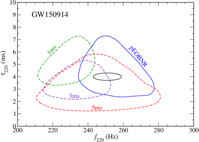
Figure 2: 90% credible interval contours for the dominant QNM, using the pEOBNR model and a damped sinusoid model at starting times $t_{\rm RD}=1,3,5$ ms after merger. The black solid line shows the 90% credible region for the frequency and decay time of the (220) QNM inferred from the posterior distributions of the remnant BH mass and spin parameters, as derived in Ref. Abbott et al. (2016c). GW150914 is consistent with the coalescence of two nonspinning BHs, with an inferred total (redshifted) mass of $M/M_{\odot}=70.6^{+4.6}_{-4.5}$, mass ratio $q=0.82^{+0.17}_{-0.20}$ and luminosity distance $D_{L}/{\rm Mpc}=410^{+160}_{-180}$ Abbott et al. (2016e).

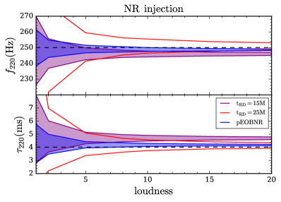
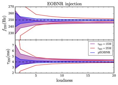
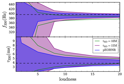
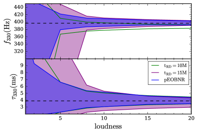
Figure 3: 95% credible interval contours for the frequency and damping time of the (220) and (330) modes of a GW event with mass ratio $q=1.5$, total (redshifted) mass $M=70M_{\odot}$ as a function of the loudness, defined as ${\rm loudness}=500{\rm Mpc}/D_{L}$. The dashed black lines corresponds to the injected values. We compare the recovery using the pEOBNR model with the one using a single damped sinusoid with starting time $t_{0}=t_{c}+t_{\rm RD}$. In the left panels we show the recovery for an NR injection, while in the right panels we show the recovery for an injection with an EOBNR waveform with the same parameters.

III.1 Putting the IMR model to test using GW150914

GW150914 Abbott et al. (2016a) was the first and, so far, loudest BBH’s GW signal detected by Advanced LIGO and Virgo. Constraints for the frequency and damping time of the dominant QNM for this event were computed in Ref. Abbott et al. (2016c). Following the latter, we use 8 s of data centered around GW150914 from both Livingston and Hanford LIGO detectors, and infer GW150914’s parameters using the pEOBNR model. In Fig. 2 we show the 90% credible intervals of the 2D PDF for the recovery of the dominant QNM frequency $f_{220}$ and damping time $\tau_{220}$. We also compare the results with the constraints that we obtain when using the two damped sinusoid model with different starting times . We also show the frequencies as inferred by assuming GR and using the posterior distributions of the remnant mass and spin parameters as derived in Ref. Abbott et al. (2016c) (black solid line). Our main conclusion is that the pEOBNR model gives constraints that are in full agreement with the ones inferred from the posterior distributions of the remnant mass and spin parameters, and even slightly stronger than the damped sinusoid model. In addition, as already emphasized, the pEOBNR model avoids intrinsic issues inherent with using a damped sinusoid model such as potential biases due a non-optimal choice of the a priori unknown starting time for the ringdown signal. In particular, one can see that choosing the damped sinusoid model to start $t_{\rm RD}=1$ ms after merger gives inconsistent results with the expected frequency and damping time, showing that this choice is too early for the start of the ringdown, something which is a priori unknown from the data alone. In addition, the uncertainty in the measurement of the time at coalescence and sky position is naturally included in the pEOBNR model, while such uncertainty cannot be easily incorporated in the damped sinusoid model (see Ref. Cabero et al. (2017) for a proposal on how to include such uncertainty).

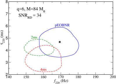
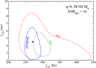
Figure 4: Left: 90% credible interval contours for the $(220)$ QNM complex frequency for NR waveform with mass ratio $q=6$, total (redshifted) mass $M=84M_{\odot}$ and IMR network SNR$\approx 70$, corresponding to an SNR in the ringdown of ${\rm SNR}_{\rm RD}\approx 34$. The black star corresponds to the injected value for the $(220)$ QNM. Right: Same, but for the recovery of the $(330)$ QNM.

III.2 Putting the IMR waveform model to test using numerical-relativity waveforms

It was recently claimed in Ref. Thrane et al. (2017) that there is an intrinsic limit in the accuracy with which one can extract QNM frequencies, when describing the post-merger signal by a sum of exponentially damped sinusoids. In particular, Ref. Thrane et al. (2017) argued that although a more sensitive detector can probe later times in the GW signal, it does not necessarily mean one can get tighter constraints on the ringdown frequencies and damping times, due to a tension between the need to maximize the SNR at which one extracts the QNM frequencies, and an optimal choice for the time at which the signal can be well-described by a sum of QNMs. The authors speculated that this effect might be due to residual nonlinearities decaying on similar timescales to the ringdown signal, but more recently Ref. Baibhav et al. (2018) argued that this effect is likely due to the increasing importance of the overtones in the large-SNR limit.

In fact, as we show below and as expected, we do not find any conclusive evidence of this limitation when using the IMR waveform at our disposal. In particular, as already emphasized, the pEOBNR model includes overtones and naturally encodes information on the starting time of the ringdown. In addition to these features, the model also includes crucial information necessary to accurately measure subdominant modes, such as time shifts between the peak of the different modes and their relative phase and amplitude difference compared to the dominant (220) mode.

To reproduce the features seen in Ref. Thrane et al. (2017) we inject an NR waveform with mass ratio $q=1.5$ (SXS:BBH:0007) and total redshifted mass $M=70M_{\odot}$ at different distances while keeping all the other parameters constant. Following Thrane et al. (2017) we define the loudness of the signal as ${\rm loudness}=500{\rm Mpc}/D_{L}$. For the injections that we consider, ${\rm loudness}=1$ corresponds to a network ${\rm SNR}\approx 50$ and ${\rm SNR}_{\rm RD}\approx 20$. We also note that, everything else being fixed, ${\rm loudness}\propto{\rm SNR}$. Following Ref. Thrane et al. (2017), and to avoid potential errors introduced by the presence of higher-modes in the NR signal, we inject the (2,2) and (3,3) modes of the NR waveform separately. To understand whether potential biases are due to residual nonlinearities in the NR waveform or simply due to a non-optimal choice of the starting time for the damped sinusoid model, we also inject the EOBNR waveform mode Pan et al. (2011) with the same parameters of the NR waveform, for which the ringdown part is exactly described by a sum of QNMs (see Eq. (1)). The injected signals are then recovered using both the pEOBNR model, which has free QNM complex frequencies, and a single damped sinusoid model, with different starting times.

Our results are summarized in Fig. 3. As expected, by increasing the loudness (i.e., increasing the SNR of the injected signal), the error decreases roughly as $1/{\rm SNR}$. As can be seen in the left panels, when recovering the NR signal with a single damped sinusoid, if one chooses a starting time too early after merger, one expects the damped sinusoid to recover inaccurate QNM frequencies, while choosing a starting time too late after merger leads to large statistical errors. We find that one needs to start the matching at a time after merger of at least $t_{\rm RD}\gtrsim 20M$ for the (220) mode and $t_{\rm RD}\gtrsim 15M$ for the (330) mode, to get unbiased frequencies and damping times. This is consistent with recent studies on the starting time of the ringdown in BBH mergers Bhagwat et al. (2017). On the other hand, the pEOBNR model recovers both the frequency and damping time of the NR waveform with a very a good accuracy, although we find a small bias of $\sim 1\%$ for the (220) frequency compared to the injected value. This is likely a systematic bias due to modeling errors in the inspiral-plunge part of the IMR model Littenberg et al. (2013). In fact, as can be seen in the right panels, when injecting the EOBNR waveform, as expected the pEOBNR model recovers unbiased frequencies and damping times while the behavior of the damped sinusoid model is similar to what we found for the NR injection, therefore no apparent sign of residual nonlinearities in the NR waveforms are found when using the damped sinusoid model. In addition, in Ref. Littenberg et al. (2013) it was shown that at sufficiently large SNRs, biases of the same order can occur for the measured BH masses when recovering a NR waveform with an EOBNRv2HM template. We expect that this error propagates to the recovered QNM frequencies, explaining the small bias we observe for the pEOBNR model. We therefore find no conclusive evidence that the limitation discussed in Ref. Thrane et al. (2017) is due to residual nonlinearities in the ringdown part of the NR waveform, and in particular we find no evidence that the IMR pEOBNR model has such limitation (aside from modeling errors).

So far, we have assumed that the different modes in the signal can be distinguished and recovered separately. In a realistic scenario one would prefer instead to use the IMR pEOBNR model against the full GW signal, since disentangling the different modes is a very challenging task that would induce unavoidable systematic errors. Therefore, in Fig. 4 we also show an example where we inject an NR waveform with all available modes (i.e., up to $\ell=8)$, for mass ratio $q=6$ (SXS:BBH:0166) and total (redshifted) mass $M=84M_{\odot}$. We consider an injection with total network ${\rm SNR}\approx 70$, corresponding to a luminosity distance $D_{L}=160{\rm Mpc}$ and ${\rm SNR}_{\rm RD}\approx 34$. We recover again the GW signal using the pEOBNR model, with all the modes available in the model, and contrast it with the recovery when using a two damped-sinusoid model, with amplitudes fitted to NRGossan et al. (2012), using different starting times. Due to the large-mass ratio, in this case there is a clear hierarchy between the amplitude of different modes, and higher modes have a non-negligible contribution to the overall waveform. For this mass ratio the peak amplitude of the (3,3)-mode is roughly $70\%$ smaller than the (2,2)-mode, as can be seen in Fig. 1, and therefore strong constraints on a second QNM can be obtained even for a reasonable SNR in the ringdown (i.e., $\approx 34$). As we see, the pEOBNR model recovers unbiased results for the ringdown frequency and damping time, even if the NR waveform includes more subdominant modes. On the other hand, when using the two damped-sinusoid model and choosing starting times that give comparable errors to the pEOBNR model, we always recover slightly biased QNM parameters. These results demonstrate the need of including more physical effects, e.g. include more modes and overtones London et al. (2014); London (2018); Cotesta et al. (2018), in the more theory-agnostic damped-sinusoid model, if one wanted to use it to get accurate and precise values for the QNM frequencies and damping times of BBHs event, and test the no-hair conjecture.

We note that at the time of this writing, no suitable NR waveform computed in alternative theories of gravity are available for testing. While the tests in this section validate our approach to constrain small deviations from GR, we do hope that further tests with non-GR waveforms will be performed in the future.

IV Testing the general relativistic no-hair conjecture

Having laid down the ability of the pEOBNR waveform model to measure the ringdown complex frequencies, we now investigate the capacity of the IMR model to detect small deviations from GR in the ringdown part of the signal using two approaches: (i) a Bayesian model selection scheme, and (ii) by directly measuring the QNM frequencies using Bayesian parameter estimation and computing the constraints on deviations from GR.

Such approaches have been used in the past Gossan et al. (2012); Meidam et al. (2014), however focusing on the damped sinusoid model, which as we have argued above, is prone to technical difficulties. Therefore, from now on, we focus solely on the IMR pEOBNR model.

IV.1 Bayesian model selection

Bayesian model selection has been extensively used in the context of testing GR Del Pozzo et al. (2011); Li et al. (2012); Gossan et al. (2012); Meidam et al. (2014), and is particularly useful to find statistical evidence for deviations from GR even when the majority of the GW events have a small SNR, and parameter estimation alone might not be enough to confidently measure such deviations. Model selection can also naturally be used to get statistical evidence from a small deviation from GR by combining the information from several observations Li et al. (2012); Meidam et al. (2014). In fact, for most of the BBH events that Advanced LIGO and Virgo is detecting, we do not expect to be able to impose strong constraints on the QNM complex frequencies Berti et al. (2016), and therefore this is the most promising avenue to detect deviations from GR, before LISA or third-generation detectors on the ground, such as Cosmic Explorer and Einstein Telescope are online.

As said above, similar studies were done in the past in Refs. Gossan et al. (2012); Meidam et al. (2014), but they focused on damped-sinusoid models, both for the injected GW signal and the waveform model used to recover it, and they were done using the PSD of Einstein Telescope. Besides the use of an IMR model to recover the signal, another crucial difference here, is that we also inject IMR waveforms. If one would do a Bayesian model selection study on such population using damped sinusoids as templates, one would need to deal with the problem of defining the optimal starting time for the ringdown, that is in general dependent on the particular binary’s configuration. Using the IMR model completely avoids this problem. In addition, a Bayesian model selection with an IMR model also naturally incorporates the consistency test that both the inspiral-plunge and merger-ringdown are consistent with GR.

In general, given some observed data $d$, the support for a given model hypotheses $\mathcal{H}$ can be quantified by integrating Eq. (4) (with $h$ replaced by $\mathcal{H}$) over $\bm{\vartheta}$:

$$p(\mathcal{H}|d)\propto\mathcal{L}(d|\mathcal{H})\times p(\mathcal{H}).$$ (6)

To compare two different model hypotheses, say $\mathcal{H}_{i}$ and $\mathcal{H}_{j}$, in light of the observed data, we compute the ratio of posterior probabilities also known as the odds ratio Del Pozzo et al. (2011); Li et al. (2012):

$$\mathcal{O}_{j}^{i}=\frac{p(\mathcal{H}_{i}|d)}{p(\mathcal{H}_{j}|d)}=\frac{p(\mathcal{H}_{i})}{p(\mathcal{H}_{j})}\frac{\mathcal{L}(d|\mathcal{H}_{i})}{\mathcal{L}(d|\mathcal{H}_{j})}=\frac{p(\mathcal{H}_{i})}{p(\mathcal{H}_{j})}B_{j}^{i}\,,$$ (7)

where $p(\mathcal{H}_{i})/p(\mathcal{H}_{j})$ is the prior odds of the two hypotheses and $B_{j}^{i}$ is the Bayes factor. In the following, we quote directly the Bayes factor, so that by construction, if $B_{j}^{i}>1(<1)$ the data prefers the model $i(j)$. Then, we need to multiply by the prior odds (which in the case of GR versus non-GR could be a large effect) to get the odds ratio.

Even though no waveform model that corresponds to a non-GR theory is currently available, we may ask: “Given the observed data, are the QNM frequencies and damping times compatible with GR?”. To address this question, we consider two different hypotheses models: (i) $\mathcal{H}_{\rm GR}$, which corresponds to the hypothesis that the events are described by EOBNR waveforms where QNM frequencies are fixed to the GR values, and (ii) $\mathcal{H}_{\rm nonGR}$, which corresponds to the hypothesis that the QNM complex frequencies are (additional) free parameters and are described by pEOBNR waveforms. Note that the latter also includes GR for a particular choice of QNM frequencies, however, even if GR is the correct theory, the model is penalized when performing Bayesian model selection due to the addition of extra parameters that are not needed to describe the data. For simplicity, in this work, the model $\mathcal{H}_{\rm nonGR}$ uses the hypothesis that only the frequencies and damping times of the (220) and (330) are not fixed by the inspiral parameters as given in GR, but all the other QNMs included in the model do (i.e., the 21-mode, 44-mode, and 55-mode and their overtones). We note that we could follow an approach similar to TIGER (Test Infrastructure for GEneral Relativity) Li et al. (2012), where all combinations of possible free parameters are included in the non-GR hypothesis. This approach is in general quite robust in finding deviations from GR even for low SNR systems, but it can be computationally expensive because several models must be analyzed. Therefore, for practical purposes, we only consider the hypothesis that the frequencies and damping times of the (220) and (330) are free at the same time.

To carry out the analysis on a reasonable timescale, we fix the sky position and the parameters influencing mostly the inspiral-plunge phase, namely the mass ratio $q$ and chirp mass $M_{c}$. Given that the inspiral is the same for both the GR (EOBNR) and non-GR (pEOBNR) hypotheses, this is a reasonable assumption that should not influence the qualitative picture of the results, especially at large SNRs, where the inspiral parameters and the sky position are measured with very good accuracy. However, the model and framework presented here are not limited to those assumptions, and we plan to relax them and do a more comprehensive analysis in the near future.

Given a detection, we compute the Bayes factor as:

$$B^{\rm nonGR}_{\rm GR}=\frac{B^{\rm nonGR}_{\rm noise}}{B^{\rm GR}_{\rm noise}}\,,$$ (8)

where $B^{\rm nonGR}_{\rm noise}$ and $B^{\rm GR}_{\rm noise}$ are the Bayes factors for $\mathcal{H}_{\rm nonGR}$ and $\mathcal{H}_{\rm GR}$ against the hypothesis that the data contain only noise, which we obtain using a nested sampling algorithm as implemented in the LIGO Algorithm Library Veitch et al. (2015).

For the catalogs of injections we construct two populations of 100 BBH sources, one with GR waveforms using the EOBNR waveform model Pan et al. (2011), that we call the GR population, and a second catalogue with the pEOBNR model with QNM frequencies given by $\sigma_{220}=\sigma^{\rm GR}_{220}(1+\delta\sigma)$ and $\sigma_{330}=\sigma^{\rm GR}_{330}(1+\delta\sigma)$ where we fixed $\delta\sigma=0.1$ (the same choice was done in Ref. Meidam et al. (2014)). Below we refer to the latter as the non-GR population. We note that this choice is not necessarily unrealistic, since deviations of $10\%$ in the QNM frequencies have been found in some alternative theories to GR. QNM frequencies of spherically symmetric solutions were computed in theories such as Einstein-Maxwell-dilaton Ferrari et al. (2001), dynamical Chern-Simons gravity Molina et al. (2010), Einstein-dilaton-Gauss-Bonnet gravity Pani and Cardoso (2009); Blazquez-Salcedo et al. (2016, 2017) and for some solutions in massive (bi)gravity Brito et al. (2013a, b); Babichev et al. (2016). On the other hand, not much progress has been made to compute QNMs for spinning BHs in alternative theories to GR, the only exception being the Kerr-Newman case in Einstein-Maxwell theory Pani et al. (2013a, b); Mark et al. (2015); Dias et al. (2015). Most of the estimates for QNMs of spinning BHs in modified gravity have instead used the connection between the light ring and QNMs Blazquez-Salcedo et al. (2016); Glampedakis et al. (2017); Jai-akson et al. (2017); Glampedakis and Pappas (2018), which is formally only valid in the eikonal $\ell\to\infty$ limit and known to fail to describe some families of QNMs when additional degrees of freedom are present Blazquez-Salcedo et al. (2016).

We draw the component (redshifted) masses of the 100 sources from a uniform distribution between 30 and 180 $M_{\odot}$ and maximum total (redshifted) mass $210M_{\odot}$. This choice implies a distribution for the mass ratios proportional to $1/q^{2}$ with a maximum value $q=6$. We draw the sky position and orientations $(\alpha,\delta,\psi,\theta)$ from uniform distributions on the sphere. The signals are distributed uniformly in volume with a network SNR for the IMR signal ranging from ${\rm SNR}=8$ to ${\rm SNR}=100$ (corresponding to luminosity distances from roughly $D_{L}=100\,{\rm Mpc}$ up to $D_{L}=5000\,{\rm Mpc}$).

We summarize the results in Fig. 5 where we show the (log) Bayes factor for the individual sources as a function of the SNR in the ringdown part of the signal only (SNR_RD). Since the sources are distributed uniformly in volume, the majority of our signals has an ${\rm SNR}_{\rm RD}<10$. In this region, there is no clear difference between the log Bayes factor for the GR and non-GR population. In fact, for ${\rm SNR}_{\rm RD}<10$, even for the non-GR population the preferred model is the GR waveform (which follows from the fact that $\ln B^{\rm nonGR}_{\rm GR}<0$ for the non-GR population). This is consistent with the fact that the GR and non-GR waveforms have the same inspiral. Therefore, since the SNR in the ringdown is small, and Bayesian model selection naturally incorporates an Occam’s razor selection, the model with fewer parameters (i.e., the GR waveform) is favored in this region. However, for ${\rm SNR}_{\rm RD}\gtrsim 15$ we see a separation between the GR injections and the non-GR injections and for ${\rm SNR}_{\rm RD}\gtrsim 25$, the non-GR waveform are always favored for the non-GR events (i.e., $\ln B^{\rm nonGR}_{\rm GR}>0$). As one would expect, the separation becomes much clearer with increasing ${\rm SNR}_{\rm RD}$. We note that the threshold ${\rm SNR}_{\rm RD}$ at which deviations from GR can be detected are dependent on the particular non-GR deviation. However, this study illustrates the nontrivial fact that even at relatively low SNRs, Bayesian model selection is able to find statistical evidence for deviations from GR.

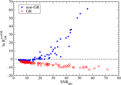
Figure 5: The log Bayes factors for individual sources. The red circles represent signals with GR waveforms (EOBNR), while the blue crosses correspond to the non-GR waveforms (pEOBNR). A separation between the two is visible for ${\rm SNR}_{\rm RD}\sim 15$, and becomes more pronounced as the SNR increases.

IV.2 Bounding free parameters of the ringdown signal

Given a set of detected GW signals from BBHs for which QNM frequencies and damping times can be measured, the natural steps to follow are to first test the compatibility of the waveform with GR using Bayesian model selection, as done in the previous subsection, and then quantify how well we can constrain deviations from GR using parameter estimation. This can be done for single GW events, but stronger constraints can be obtained by combining the information from all the detections as shown in Ref. Meidam et al. (2014). There, two different approaches were proposed: (i) the odds ratio obtained in the previous subsection can be combined by just multiplying the odds ratio coming from all the events, thus allowing to get stronger evidence for or against GR. For a large group of $\mathcal{N}$ identical events, this method effectively improves the SNR of the single event case by a factor $\sim\mathcal{N}^{1/4}$ Yang et al. (2017); and (ii) assuming that the Bayesian model selection test gives no evidence for deviations from GR, one combines the posterior density distributions for $\delta\sigma_{\ell m}$, which measures the fractional deviation from the QNM complex frequencies of a Kerr BH in GR:

$$\sigma_{lm}=\sigma^{\rm GR}_{lm}(1+\delta\sigma_{lm})\,.$$ (9)

Given that in GR $\delta\sigma_{lm}=0$, the information from multiple events can be combined by multiplying the posterior density distributions of all detections as

$$p(\delta\sigma|\mathcal{H},d_{1},d_{2},d_{3},\ldots,\mathcal{N})=\frac{1}{p(\delta\sigma)^{1-\mathcal{N}}}\prod_{A=1}^{\mathcal{N}}p(\delta\sigma|\mathcal{H},d_{A})\,,$$ (10)

where $\mathcal{N}$ denotes the number of detections. For a large group of $\mathcal{N}$ identical events, the width of this PDF decreases as $\sim\mathcal{N}^{-1/2}$. We emphasize that when using Eq. (10) one assumes that the value of $\delta\sigma_{lm}$ is the same across all events. Therefore, since for generic theories of gravity the deviations $\delta\sigma_{\ell m}$ could also be a function of the final BH mass, spin and any other charges that may be present in the correct theory of gravity, constraints obtained using this method only make sense if no evidence for deviations from GR are found after performing the Bayesian model selection test Meidam et al. (2014).

More recently Ref. Yang et al. (2017) proposed an alternative hypothesis testing method that makes use of the combined information from multiple detections and could, in principle, enhance the efficiency to detect sub-leading modes compared to the Bayesian model selection method used in Ref. Meidam et al. (2014). This method proposes to make full use of the information coming from the measured BBH parameters, to coherently sum the ringdown signal of a target mode from multiple events. It could, in an ideal scenario, effectively improve the SNR of a single event by a factor $\sim\mathcal{N}^{1/2}$, assuming $\mathcal{N}$ identical events Yang et al. (2017). However, implementing the coherent stacking method of Ref. Yang et al. (2017) is technically very challenging. Here, we follow Ref. Meidam et al. (2014) and use Eq. (10) to combine the information from a population of detected BBHs.

Since for each event we sample on the parameter $\sigma_{lm}$, we compute the PDFs for $\delta\sigma_{lm}$ a posteriori by using Eq. (9). To compute $\sigma^{\rm GR}_{lm}$ we use the fitting formulas in Ref. Berti et al. (2006) (see Appendix E therein) where for the spin and mass of the final BH we employ the fitting formulas in Ref. Pan et al. (2011) [see Eqs. (29a) and (29b) therein]. The results for the constraints on the parameters $\delta\sigma_{\ell m}$, when considering the GR BBH population described in the previous subsection, are displayed in Fig. 6. In particular, we show how the median and $95\%$ confidence interval evolve with the number of detections ordered randomly. Although the constraints from a single event can be quite uninformative, when all sources are taken into account the $95\%$ confidence interval shrinks to a maximum error away from the median of $\sim 0.7\%$, $\sim 1.6\%$ and $\sim 2.4\%$ , for $\delta f_{220}$, $\delta f_{330}$ and $\delta\tau_{220}$, respectively. As expected and as shown in Fig. 7, we find that at large enough $\mathcal{N}$, the error decreases approximately as $\mathcal{N}^{-1/2}$. Overall, our results are consistent with previous studies Meidam et al. (2014), although we remind that Ref. Meidam et al. (2014) used damped sinusoids for both the injected GW signal and the recovery, while we injected and recovered with an IMR waveform that consistently includes time and phase shifts between QNMs.

It is worth noticing that if we consider only events with (total) SNR below 30 (which accounts for 60 events of the entire population), and combine them, we obtain at $95\%$ confidence that the maximum errors away from the median are $\sim 1.7\%$ $\sim 5.3\%$ and $\sim 6.7\%$, for $\delta f_{220}$, $\delta f_{330}$ and $\delta\tau_{220}$, respectively. Moreover, we find that $\delta f_{220}$ is the quantity for which we gain less by combining several events, because it is the best measured quantity — e.g., for some individual events with SNR less than 30, we get errors on the order of $\sim 5\%$. By contrast, if we consider only events with SNR less than 30, the errors of $\delta f_{330}$ and $\delta\tau_{220}$ for individual events are always larger than $20\%$.

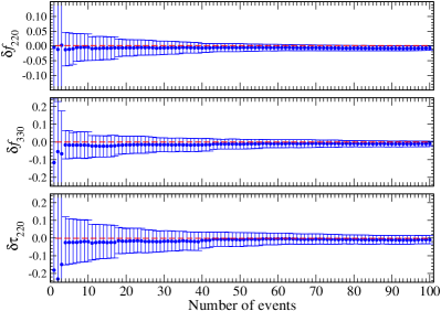
Figure 6: Evolution of the medians and $95\%$ confidence intervals for deviations on the QNM frequencies as a function of the number of events included in the computation of the joint posterior density distributions, for the population of GR BBHs described in the subsection IV.1.

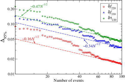
Figure 7: Evolution of the width of the $95\%$ confidence intervals ($\Delta_{95\%}$) shown in Fig. 6 as a function of the number of events $\mathcal{N}$. Note that a log-log scale is used in this plot to make apparent the power-law scaling of the error at large $\mathcal{N}$. The dashed lines scale as $\sim\mathcal{N}^{-1/2}$ showing that at large enough $\mathcal{N}$, the error decreases approximately as $\mathcal{N}^{-1/2}$.

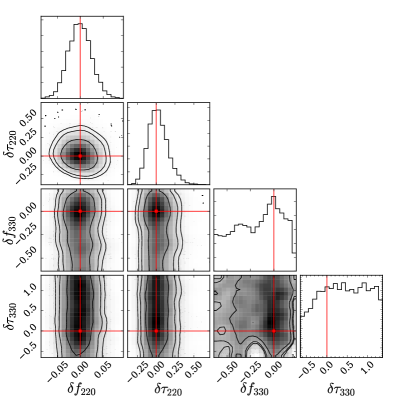
Figure 8: Posterior density distributions of the quantities $\delta f_{220}$, $\delta f_{330}$, $\delta\tau_{220}$ and $\delta\tau_{330}$ for a single GW150914-like event with mass ratio $q=1.5$, total (redshifted) mass $M=70M_{\odot}$, luminosity distance $D_{L}=500{\rm Mpc}$ and inclination $\theta=2.2\,{\rm rad}$. The red solid lines correspond to the injected values.

Quite interestingly, using Eq. (10) for identical GW150914-like events with mass ratio $q=1.5$, total (redshifted) mass $M=70M_{\odot}$, luminosity distance $D_{L}=500{\rm Mpc}$ and inclination $\theta=2.2\,{\rm rad}$ (i.e., the EOBNR injection with loudness$=1$ in Fig. 3), one can estimate how many such events would be needed to test the BH’s no-hair conjecture with Advanced LIGO and Virgo at design sensitivity, assuming that GR is the correct theory. The posterior density distributions for a single event is shown in Fig. 8, where we see that no relevant constraints can be put on the frequency of the $(330)$ with a single event, however by combining several observations one can get interesting constraints. The results are summarized in Fig. 9 where we plot the 2-$\sigma$ errors for $\delta f_{220}$, $\delta f_{330}$ and $\delta\tau_{220}$. We find that we would need $\sim 20$ GW150914-like events to constrain the frequency of the (220) mode by $1\%$ at the 2-$\sigma$ level, while to constrain the damping time of the (220) mode by $5\%$ one would need $\sim 23$ such events. On the other hand, to constrain the frequency of the (330) by $5\%$ we would need at least $\sim 32$ events, and we note that this last number is highly dependent on the BBH mass ratio and inclination. From the expected rates for GW150914-like events Abbott et al. (2016f), one can conclude that, in the best case scenario, with one year of observations at design sensitivity one could have $\mathcal{O}(10)$ GW150914-like events, therefore being able to measure $f_{330}$ with an error of the order of $10\%$ at the 2-$\sigma$ level, while $f_{220}$ and $\tau_{220}$ would be measured with 2-$\sigma$ errors of less than $2\%$ and $10\%$, respectively.

A concrete way to visualize what this means in terms of testing the no-hair conjecture is to relate the measured QNM frequencies and damping times with the mass and spin of a Kerr BH in GR, as done in Refs. Kamaretsos et al. (2012); Gossan et al. (2012). Using the fits of Ref. Berti et al. (2006), one can draw bands for each measured QNM parameter in the mass versus spin plane. If the bands do not intersect then one can invalidate GR or conclude that the final object is not a BH. For the GW150914-like events discussed above, our results are summarized in Fig. 10 where we show the projections of the $95\%$ confidence intervals for $(f_{22},f_{33},\tau_{22})$ in the mass versus spin of the final compact object, when considering only one event and, for illustration, when combining $30$ identical events. As one can see, the bands intersect perfectly at the injected value (yellow star in Fig. 10) with a significant decrease of the width of the bands when combining several events. This illustrates how combining several events can be used to severely constrain deviations from GR.

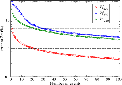
Figure 9: Evolution of 2-$\sigma$ error of the joint posterior density distributions for the quantities $\delta f_{220}$, $\delta f_{330}$, $\delta\tau_{220}$, assuming identical GW150914-like events with posterior density distributions for a single event given in Fig. 8. The dashed black lines correspond to errors of $5\%$ and $1\%$.

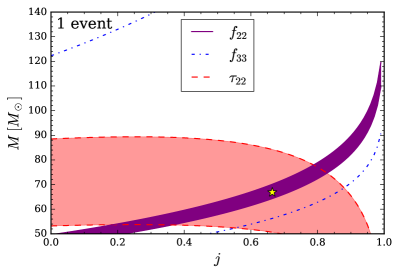
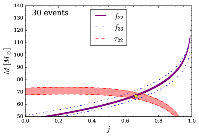
Figure 10: Left: Projections of the $95\%$ confidence intervals for $(f_{22},f_{33},\tau_{22})$ in the mass ($M$) versus dimensionless spin ($j\equiv J/M^{2}$) of the final compact object for a GW150914-like event. The yellow star corresponds to the injected value. Right: Same, but after combining 30 GW150914-like identical events.

V Outlook

We investigated the advantages of using IMR waveforms, with respect to damped-sinusoid models, to measure ringdown frequencies and damping times in the post-merger signal of a compact-object coalescence. To address this goal, we built a parameterized multipolar IMR waveform model within the EOB formalism (pEOBNR), and investigated its ability in measuring the QNM complex frequencies in GW150914, and in several synthetic GW signals injected in Gaussian noise.

We found the following important advantages: (i) using an IMR model, calibrated to NR waveforms, one does not need to define an a priori unknown starting time at which the signal can be described as a sum of exponentially damped sinusoids Gossan et al. (2012); Meidam et al. (2014); Cabero et al. (2017); Bhagwat et al. (2017); Baibhav et al. (2018); London (2018), therefore avoiding potential biases due to a non-optimal choice of the ringdown starting time Thrane et al. (2017); (ii) the IMR model avoids technical issues inherent to assuming a waveform with a cutoff at a particular time, namely the need to know in advance the sky position and time at coalescence Abbott et al. (2016c); Cabero et al. (2017); (iii) the IMR model naturally includes important physics, such as phase shifts between different modes, their relative amplitudes and the presence of overtones Buonanno et al. (2007); Pan et al. (2011); and (iv) the IMR model generically leads to stronger constraints on the QNM frequencies compared to what can be achieved with a damped-sinusoid model.

The approach that we here presented should also be seen as complementary to previous works on the subject. Besides directly measuring the ringdown frequencies, our IMR model can also be used to validate the results obtained with the more agnostic damped-sinusoid models. In particular, as we showed, the pEOBNR model already provides very interesting constraints on the frequency and damping time of the dominant QNM of GW150914 Abbott et al. (2016a).

This work can be improved in several fronts and should be seen as a first step toward more accurate waveform models that allow to measure deviations from GR. Although we presented results using a nonspinning BBH waveform model, the extension to nonprecessing, spinning BBHs is straightforward and will be done in the future, using the recently developed multipolar EOBNR model with spins aligned/anti-aligned with the direction perpendicular to the orbital plane Cotesta et al. (2018). Given that EOBNR models naturally encodes time shifts between different modes and their relative amplitudes and phases, it could in principle be used as a starting point to perform the coherent stacking proposed in Refs. Yang et al. (2017); Da Silva Costa et al. (2017). A proper implementation of the method is, however, challenging and requires further work. The IMR model here presented could also be extended to allow GR deviations in the inspiral phase. In addition, further work in detector noise modelling is needed to handle non-Gaussianities in the data. We do note that longer waveform models, such as the ones generated with our IMR model, are in general more robust against deviations from Gaussian noise than shorter waveform models, such as the damped-sinusoid models. We hope to come back to these relevant issues in the near future. Finally, we note that a MCMC parameter estimation run using the pEOBNR model is in general much slower than using the much simpler damped sinusoid model. However, as already done in the literature (see e.g. Ref. Purrer (2016); Bohé et al. (2017)), efficient waveforms can be obtained building a reduce-order-model of pEOBNR waveforms, which we plan to develop in the near future.

References

- Abbott et al. (2016a) B. P. Abbott et al. (Virgo, LIGO Scientific), Phys. Rev. Lett. 116, 061102 (2016a), arXiv:1602.03837 [gr-qc] .
- Abbott et al. (2016b) B. P. Abbott et al. (Virgo, LIGO Scientific), Phys. Rev. Lett. 116, 241103 (2016b), arXiv:1606.04855 [gr-qc] .
- Abbott et al. (2017a) B. P. Abbott et al. (VIRGO, LIGO Scientific), Phys. Rev. Lett. 118, 221101 (2017a), arXiv:1706.01812 [gr-qc] .
- Abbott et al. (2017b) B. P. Abbott et al. (Virgo, LIGO Scientific), Astrophys. J. 851, L35 (2017b), arXiv:1711.05578 [astro-ph.HE] .
- Abbott et al. (2017c) B. P. Abbott et al. (Virgo, LIGO Scientific), Phys. Rev. Lett. 119, 141101 (2017c), arXiv:1709.09660 [gr-qc] .
- Abbott et al. (2016c) B. P. Abbott et al. (Virgo, LIGO Scientific), Phys. Rev. Lett. 116, 221101 (2016c), arXiv:1602.03841 [gr-qc] .
- Abbott et al. (2016d) B. P. Abbott et al. (Virgo, LIGO Scientific), Phys. Rev. X6, 041015 (2016d), arXiv:1606.04856 [gr-qc] .
- Abbott et al. (2017d) B. P. Abbott et al. (Virgo, LIGO Scientific), Phys. Rev. Lett. 119, 161101 (2017d), arXiv:1710.05832 [gr-qc] .
- Abbott et al. (2018) B. P. Abbott et al. (Virgo, LIGO Scientific), (2018), arXiv:1805.11579 [gr-qc] .
- Kerr (1963) R. P. Kerr, Phys. Rev. Lett. 11, 237 (1963).
- Will (2014) C. M. Will, Living Rev. Rel. 17, 4 (2014), arXiv:1403.7377 [gr-qc] .
- Berti et al. (2015) E. Berti et al., Class. Quant. Grav. 32, 243001 (2015), arXiv:1501.07274 [gr-qc] .
- Mazur and Mottola (2004) P. O. Mazur and E. Mottola, Proc. Nat. Acad. Sci. 101, 9545 (2004), arXiv:gr-qc/0407075 [gr-qc] .
- Visser and Wiltshire (2004) M. Visser and D. L. Wiltshire, Class. Quant. Grav. 21, 1135 (2004), arXiv:gr-qc/0310107 [gr-qc] .
- Liebling and Palenzuela (2012) S. L. Liebling and C. Palenzuela, Living Rev. Rel. 15, 6 (2012), arXiv:1202.5809 [gr-qc] .
- Vishveshwara (1970) C. V. Vishveshwara, Nature 227, 936 (1970).
- Press (1971) W. H. Press, Astrophys. J. 170, L105 (1971).
- Chandrasekhar and Detweiler (1975) S. Chandrasekhar and S. L. Detweiler, Proc.Roy.Soc.Lond. A344, 441 (1975).
- Israel (1967) W. Israel, Phys. Rev. 164, 1776 (1967).
- Carter (1971) B. Carter, Phys. Rev. Lett. 26, 331 (1971).
- Hawking (1972) S. W. Hawking, Commun. Math. Phys. 25, 152 (1972).
- Robinson (1975) D. C. Robinson, Phys. Rev. Lett. 34, 905 (1975).
- Dreyer et al. (2004) O. Dreyer, B. J. Kelly, B. Krishnan, L. S. Finn, D. Garrison, and R. Lopez-Aleman, Class. Quant. Grav. 21, 787 (2004), arXiv:gr-qc/0309007 [gr-qc] .
- Berti et al. (2006) E. Berti, V. Cardoso, and C. M. Will, Phys. Rev. D73, 064030 (2006), arXiv:gr-qc/0512160 [gr-qc] .
- Gossan et al. (2012) S. Gossan, J. Veitch, and B. S. Sathyaprakash, Phys. Rev. D85, 124056 (2012), arXiv:1111.5819 [gr-qc] .
- Meidam et al. (2014) J. Meidam, M. Agathos, C. Van Den Broeck, J. Veitch, and B. S. Sathyaprakash, Phys. Rev. D90, 064009 (2014), arXiv:1406.3201 [gr-qc] .
- Yang et al. (2017) H. Yang, K. Yagi, J. Blackman, L. Lehner, V. Paschalidis, F. Pretorius, and N. Yunes, Phys. Rev. Lett. 118, 161101 (2017), arXiv:1701.05808 [gr-qc] .
- Da Silva Costa et al. (2017) C. F. Da Silva Costa, S. Tiwari, S. Klimenko, and F. Salemi, (2017), arXiv:1711.00551 [gr-qc] .
- Cardoso and Gualtieri (2016) V. Cardoso and L. Gualtieri, Class. Quant. Grav. 33, 174001 (2016), arXiv:1607.03133 [gr-qc] .
- Berti et al. (2007a) E. Berti, J. Cardoso, V. Cardoso, and M. Cavaglia, Phys. Rev. D76, 104044 (2007a), arXiv:0707.1202 [gr-qc] .
- Bhagwat et al. (2016) S. Bhagwat, D. A. Brown, and S. W. Ballmer, Phys. Rev. D94, 084024 (2016), [Erratum: Phys. Rev.D95,no.6,069906(2017)], arXiv:1607.07845 [gr-qc] .
- Berti et al. (2016) E. Berti, A. Sesana, E. Barausse, V. Cardoso, and K. Belczynski, Phys. Rev. Lett. 117, 101102 (2016), arXiv:1605.09286 [gr-qc] .
- Maselli et al. (2017) A. Maselli, K. Kokkotas, and P. Laguna, Phys. Rev. D95, 104026 (2017), arXiv:1702.01110 [gr-qc] .
- Cabero et al. (2017) M. Cabero, C. D. Capano, O. Fischer-Birnholtz, B. Krishnan, A. B. Nielsen, and A. H. Nitz, (2017), arXiv:1711.09073 [gr-qc] .
- Buonanno and Damour (1999) A. Buonanno and T. Damour, Phys. Rev. D59, 084006 (1999), arXiv:gr-qc/9811091 [gr-qc] .
- Buonanno and Damour (2000) A. Buonanno and T. Damour, Phys. Rev. D62, 064015 (2000), arXiv:gr-qc/0001013 [gr-qc] .
- Pan et al. (2011) Y. Pan, A. Buonanno, M. Boyle, L. T. Buchman, L. E. Kidder, H. P. Pfeiffer, and M. A. Scheel, Phys. Rev. D84, 124052 (2011), arXiv:1106.1021 [gr-qc] .
- Thrane et al. (2017) E. Thrane, P. D. Lasky, and Y. Levin, Phys. Rev. D96, 102004 (2017), arXiv:1706.05152 [gr-qc] .
- Barausse et al. (2012) E. Barausse, A. Buonanno, S. A. Hughes, G. Khanna, S. O’Sullivan, and Y. Pan, Phys. Rev. D85, 024046 (2012), arXiv:1110.3081 [gr-qc] .
- Mroue et al. (2013) A. H. Mroue et al., Phys. Rev. Lett. 111, 241104 (2013), arXiv:1304.6077 [gr-qc] .
- Julié and Deruelle (2017) F.-L. Julié and N. Deruelle, Phys. Rev. D95, 124054 (2017), arXiv:1703.05360 [gr-qc] .
- Julié (2018) F.-L. Julié, Phys. Rev. D97, 024047 (2018), arXiv:1709.09742 [gr-qc] .
- Kamaretsos et al. (2012) I. Kamaretsos, M. Hannam, S. Husa, and B. S. Sathyaprakash, Phys. Rev. D85, 024018 (2012), arXiv:1107.0854 [gr-qc] .
- London et al. (2014) L. London, D. Shoemaker, and J. Healy, Phys. Rev. D90, 124032 (2014), [Erratum: Phys. Rev.D94,no.6,069902(2016)], arXiv:1404.3197 [gr-qc] .
- London (2018) L. T. London, (2018), arXiv:1801.08208 [gr-qc] .
- Buonanno et al. (2007) A. Buonanno, G. B. Cook, and F. Pretorius, Phys. Rev. D75, 124018 (2007), arXiv:gr-qc/0610122 [gr-qc] .
- Berti et al. (2007b) E. Berti, V. Cardoso, J. A. Gonzalez, U. Sperhake, M. Hannam, S. Husa, and B. Bruegmann, Phys. Rev. D76, 064034 (2007b), arXiv:gr-qc/0703053 [GR-QC] .
- Bayes and Price (1763) T. Bayes and R. Price, Phil. Trans. Roy. Soc. Lond. 53, 370 (1763).
- Jaynes (2003) E. T. Jaynes, Probability Theory: The Logic of Science, edited by G. L. Bretthorst (Cambridge University Press, Cambridge, 2003).
- Veitch et al. (2015) J. Veitch et al., Phys.Rev. D91, 042003 (2015), arXiv:1409.7215 [gr-qc] .
- Finn (1992) L. S. Finn, Phys. Rev. D46, 5236 (1992), arXiv:gr-qc/9209010 [gr-qc] .
- Shoemaker (2010) D. Shoemaker (LIGO Collaboration), “Advanced LIGO anticipated sensitivity curves,” (2010), LIGO Document T0900288-v3.
- Manzotti and Dietz (2012) A. Manzotti and A. Dietz, ArXiv e-prints (2012), arXiv:1202.4031 [gr-qc] .
- Abbott et al. (2016e) B. P. Abbott et al. (Virgo, LIGO Scientific), Phys. Rev. Lett. 116, 241102 (2016e), arXiv:1602.03840 [gr-qc] .
- Baibhav et al. (2018) V. Baibhav, E. Berti, V. Cardoso, and G. Khanna, Phys. Rev. D97, 044048 (2018), arXiv:1710.02156 [gr-qc] .
- Bhagwat et al. (2017) S. Bhagwat, M. Okounkova, S. W. Ballmer, D. A. Brown, M. Giesler, M. A. Scheel, and S. A. Teukolsky, (2017), arXiv:1711.00926 [gr-qc] .
- Littenberg et al. (2013) T. B. Littenberg, J. G. Baker, A. Buonanno, and B. J. Kelly, Phys. Rev. D87, 104003 (2013), arXiv:1210.0893 [gr-qc] .
- Cotesta et al. (2018) R. Cotesta, A. Buonanno, A. Bohe, A. Taracchini, I. Hinder, and S. Ossokine, (2018), arXiv:1803.10701 [gr-qc] .
- Del Pozzo et al. (2011) W. Del Pozzo, J. Veitch, and A. Vecchio, Phys. Rev. D83, 082002 (2011), arXiv:1101.1391 [gr-qc] .
- Li et al. (2012) T. G. F. Li, W. Del Pozzo, S. Vitale, C. Van Den Broeck, M. Agathos, J. Veitch, K. Grover, T. Sidery, R. Sturani, and A. Vecchio, Phys. Rev. D85, 082003 (2012), arXiv:1110.0530 [gr-qc] .
- Ferrari et al. (2001) V. Ferrari, M. Pauri, and F. Piazza, Phys. Rev. D63, 064009 (2001), arXiv:gr-qc/0005125 [gr-qc] .
- Molina et al. (2010) C. Molina, P. Pani, V. Cardoso, and L. Gualtieri, Phys. Rev. D81, 124021 (2010), arXiv:1004.4007 [gr-qc] .
- Pani and Cardoso (2009) P. Pani and V. Cardoso, Phys. Rev. D79, 084031 (2009), arXiv:0902.1569 [gr-qc] .
- Blazquez-Salcedo et al. (2016) J. L. Blazquez-Salcedo, C. F. B. Macedo, V. Cardoso, V. Ferrari, L. Gualtieri, F. S. Khoo, J. Kunz, and P. Pani, Phys. Rev. D94, 104024 (2016), arXiv:1609.01286 [gr-qc] .
- Blazquez-Salcedo et al. (2017) J. L. Blazquez-Salcedo, F. S. Khoo, and J. Kunz, Phys. Rev. D96, 064008 (2017), arXiv:1706.03262 [gr-qc] .
- Brito et al. (2013a) R. Brito, V. Cardoso, and P. Pani, Phys. Rev. D88, 023514 (2013a), arXiv:1304.6725 [gr-qc] .
- Brito et al. (2013b) R. Brito, V. Cardoso, and P. Pani, Phys. Rev. D87, 124024 (2013b), arXiv:1306.0908 [gr-qc] .
- Babichev et al. (2016) E. Babichev, R. Brito, and P. Pani, Phys. Rev. D93, 044041 (2016), arXiv:1512.04058 [gr-qc] .
- Pani et al. (2013a) P. Pani, E. Berti, and L. Gualtieri, Phys. Rev. Lett. 110, 241103 (2013a), arXiv:1304.1160 [gr-qc] .
- Pani et al. (2013b) P. Pani, E. Berti, and L. Gualtieri, Phys. Rev. D88, 064048 (2013b), arXiv:1307.7315 [gr-qc] .
- Mark et al. (2015) Z. Mark, H. Yang, A. Zimmerman, and Y. Chen, Phys. Rev. D91, 044025 (2015), arXiv:1409.5800 [gr-qc] .
- Dias et al. (2015) O. J. C. Dias, M. Godazgar, and J. E. Santos, Phys. Rev. Lett. 114, 151101 (2015), arXiv:1501.04625 [gr-qc] .
- Glampedakis et al. (2017) K. Glampedakis, G. Pappas, H. O. Silva, and E. Berti, Phys. Rev. D96, 064054 (2017), arXiv:1706.07658 [gr-qc] .
- Jai-akson et al. (2017) P. Jai-akson, A. Chatrabhuti, O. Evnin, and L. Lehner, Phys. Rev. D96, 044031 (2017), arXiv:1706.06519 [gr-qc] .
- Glampedakis and Pappas (2018) K. Glampedakis and G. Pappas, Phys. Rev. D97, 041502 (2018), arXiv:1710.02136 [gr-qc] .
- Abbott et al. (2016f) B. P. Abbott et al. (Virgo, LIGO Scientific), Astrophys. J. 833, L1 (2016f), arXiv:1602.03842 [astro-ph.HE] .
- Purrer (2016) M. Purrer, Phys. Rev. D93, 064041 (2016), arXiv:1512.02248 [gr-qc] .
- Bohé et al. (2017) A. Bohé et al., Phys. Rev. D95, 044028 (2017), arXiv:1611.03703 [gr-qc] .