Python Framework for HP Adaptive Discontinuous Galerkin Method for Two Phase Flow in Porous Media

Abstract

In this paper we present a framework for solving two phase flow problems in porous media. The discretization is based on a Discontinuous Galerkin method and includes local grid adaptivity and local choice of polynomial degree. The method is implemented using the new Python frontend Dune-FemPy to the open source framework Dune. The code used for the simulations is made available as Jupyter notebook and can be used through a Docker container. We present a number of time stepping approaches ranging from a classical IMPES method to fully coupled implicit scheme. The implementation of the discretization is very flexible allowing for test different formulations of the two phase flow model and adaptation strategies.

Keywords: DG, hp-adaptivity, Two-phase flow, IMPES, Fully implicit, Dune, Python, Porous media

1 Introduction

Simulation of multi-phase flows and transport processes in porous media requires careful numerical treatment due to the strong heterogeneity of the underlying porous medium. The spatial discretization requires locally conservative methods in order to be able to follow small concentrations [4]. Discontinuous Galerkin (DG) methods, Finite Volume methods and Mixed Finite Element methods are examples of discretization techniques achieving local conservation at the element level [16]. Application of DG methods to incompressible two-phase flow started within the framework provided by a decoupled approach called Implicit Pressure Explicit Saturation (IMPES) where first a pressure equation is solved implicitly and then the saturation is advanced by an explicit time stepping scheme. Upwinding, slope limiting techniques, and sometimes $\mathbb{H}$(div)-projection were required in order to remove unphysical oscillations and to ensure convergence to a solution.

In the fully implicit and fully coupled approach, the mass balances are usually discretized in time by the implicit Euler method, resulting in a fully coupled system of nonlinear equations that has to be solved at each time step. The main advantage of a fully implicit scheme is the possibility of using significantly larger time step sizes, which can be crucial in view of long-term scenarios like atomic waste disposal. Commonly, rather simple, yet robust space-discretization schemes, like cell-centered or vertex-centered finite volume schemes, are used [4, 6]. Fully implicit DG schemes have been proposed in [17] and [18], where the schemes are formulated in two space dimensions for incompressible fluid phases and numerical tests are performed without any kind of adaptivity.

Bastian introduced in [5] a fully coupled symmetric interior penalty DG scheme for incompressible two-phase flow based on a wetting-phase potential and capillary potential formulation. Discontinuity in capillary-pressure functions is taken into account by incorporating the interface conditions into the penalty terms for the capillary potential. Heterogeneity in absolute or intrinsic permeability is treated by weighted averages. A higher-order diagonally implicit Runge-Kutta method in time is used and there is neither post processing of the velocity nor slope limiting. Only piecewise linear and piecewise quadratic functions are employed and no adaptive method is considered.

A general abstract framework allowing for an a-posteriori estimator for porous-media two-phase flow problem was introduced by Vohralik et al. [31]. This paved the way for an h-adaptive strategy for homogeneous two-phase flow problems [11]. However, it has not been applied to DG methods so far.

Finally, Darmofal et al. introduced recently a space-time discontinuous Galerkin h-adaptive framework for 2d reservoir flows. Implicit estimators are derived through the use of dual problems [7, 8] and a higher-order discretization is performed on anisotropic, unstructured meshes. Unfortunately, application to 3d problems and hp-adaptive strategies haven’t been considered yet.

In this paper, we implement and evaluate numerically interior penalty DG methods for incompressible, immiscible, two-phase flow. We consider strongly heterogeneous porous media, anisotropic permeability tensors and discontinuous capillary-pressure functions. We write the system in terms of a phase-pressure/phase-saturation formulation.

Adams-Moulton schemes of first or second order in time are combined with an Interior Penalty DG discretization in space. This implicit space time discretization leads to a fully coupled nonlinear system requiring to build a Jacobian matrix at each time step for the Newton-Raphson method.

This paper extends our previous work in [22, 23] and [24]. We consider here new hp-adaptive strategies and compare the fully implicit scheme with the iterative IMPES scheme and the implicit iterative scheme. The implicit iterative scheme is based on the iterative IMPES approach presented in [28] and treats the capillary pressure term implicitly to ensure stability. We also provide a more comprehensive model framework allowing to conveniently implement and compare various two-phase flow formulations.

The implementation is based on the open-source PDE software framework Dune-FemPy, which is a Python frontend for Dune-Fem [13] based on the new Dune-Python module [15] and which adds support for the Unified Form Language [3]. It allows for a compact, legible presentation of the different discretizations under consideration. We combine Dune-FemPy with Jupyter [27] and Docker [9] to ensure reproducibility of our numerical experiments. The adaptive grid implementation is based on Dune-Alugrid [2] and parts of the stabilization mechanisms used are provided by Dune-Fem-DG [14].

The rest of this document is organised as follows. In Section 2, we describe the two-phase flow model. The DG discretization is introduced in Section 3. Numerical examples are provided in Section 4. Conclusions are drawn in the last section.

2 Mathematical Model

This section introduces the mathematical formulation of a two-phase porous-media flow. In all that follows, we assume that the flow is immiscible and incompressible with no mass transfer between phases.

2.1 Two-phase flow formulation

Let $\Omega$ be a polygonal bounded domain in $\mathbb{R}^{d}$, $d\in\{2,3\}$, with Lipschitz boundary $\partial\Omega$ and let $T\in\mathbb{R}_{+}$. The flow of the wetting phase (e.g. water) and the nonwetting phase (e.g. oil, gas) is described by Darcy’s law and the continuity equation (e.g. balance of mass) for each phase $\alpha\in\{w,n\}$[21]. In all that follows, we denote with subscript $w$ the wetting phase and with subscript $n$ the nonwetting phase. The unknown variables are the phase pressures $p_{w},\ p_{n}\mathrel{\mathop{\mathchar 58\relax}}\Omega\times(0,T)\rightarrow\mathbb{R}$ and the phase saturations $s_{w},\ s_{n}\mathrel{\mathop{\mathchar 58\relax}}\Omega\times(0,T)\rightarrow\mathbb{R}$. For each phase $\alpha\in\{w,n\}$, the Darcy velocity $\mathbf{v}_{\alpha}\mathrel{\mathop{\mathchar 58\relax}}\Omega\times(0,T)\rightarrow\mathbb{R}^{d}$ is given by

$$\mathbf{v}_{\alpha}=-\lambda_{\alpha}\mathbb{K}(\nabla p_{\alpha}-\rho_{\alpha}\mathbf{g})\quad\quad\mbox{in}\ \Omega\times(0,T)$$ (1)

where $\lambda_{\alpha}\mathrel{\mathop{\mathchar 58\relax}}\Omega\times(0,T)\rightarrow\mathbb{R}$ is the phase mobility, $\mathbb{K}\mathrel{\mathop{\mathchar 58\relax}}\Omega\rightarrow\mathbb{R}^{d\times d}$ is the absolute or intrinsic permeability tensor of the porous medium, $\rho_{\alpha}\mathrel{\mathop{\mathchar 58\relax}}\Omega\times(0,T)\rightarrow\mathbb{R}$ is the phase density, and $\mathbf{g}\in\mathbb{R}^{d}$ is the constant gravitational vector.
Phase mobilities $\lambda_{\alpha}\mathrel{\mathop{\mathchar 58\relax}}\Omega\times(0,T)\rightarrow\mathbb{R}$ are defined by

$$\lambda_{\alpha}=\frac{k_{r\alpha}}{\mu_{\alpha}}\mbox{, }\quad\alpha\in\{w,n\},$$ (2)

where $\mu_{\alpha}$ is the constant phase viscosity and $k_{r\alpha}\mathrel{\mathop{\mathchar 58\relax}}\Omega\times(0,T)\rightarrow\mathbb{R}$ is the relative permeability of phase $\alpha$. The relative permeabilities are functions that depend nonlinearly on the phase saturation (i.e. $k_{r\alpha}=k_{r\alpha}(s_{\alpha})$). Models for the relative permeability are the van-Genuchten model [30] and the Brooks-Corey model [10]. For example, in the Brooks-Corey model,

$$k_{rw}(s_{n,e})=(1-s_{n,e})^{\frac{2+3\theta}{\theta}}\mbox{,}\hskip 11.38109ptk_{rn}(s_{n,e})=(s_{n,e})^{2}(1-(1-s_{n,e})^{\frac{2+\theta}{\theta}}),$$ (3)

where the effective saturation $s_{\alpha,e}$ is

$$s_{\alpha,e}=\frac{s_{\alpha}-s_{\alpha,r}}{1-s_{w,r}-s_{n,r}},\hskip 11.38109pt\forall\alpha\in\{w,n\}.$$ (4)

Here, $s_{\alpha,r}$, $\alpha\in\{w,n\}$, are the phase residual saturations. The parameter $\theta\in[0.2,3.0]$ is a result of the inhomogeneity of the medium.
For each phase $\alpha\in\{w,n\}$, the balance of mass yields the saturation equation

$$\phi\frac{\partial(\rho_{\alpha}s_{\alpha})}{\partial t}+\nabla\cdot(\rho_{\alpha}\mathbf{v}_{\alpha}) =\rho_{\alpha}q_{\alpha},$$ (5)

where $\phi\mathrel{\mathop{\mathchar 58\relax}}\Omega\rightarrow\mathbb{R}$ is the porosity, $q_{\alpha}\mathrel{\mathop{\mathchar 58\relax}}\Omega\times(0,T)\rightarrow\mathbb{R}$ is a source or sink term (e.g. wells located inside the domain in the case of a reservoir problem).
In addition to (1) and (5) the following closure relations must also be satisfied:

$$s_{w}+s_{n} =1,$$ (6)

$$p_{n}-p_{w} =p_{c}(s_{n}),$$ (7)

where $p_{c}(s_{n})\mathrel{\mathop{\mathchar 58\relax}}\Omega\times(0,T)\rightarrow\mathbb{R}$ is the capillary pressure, a function of the phase saturation. For the Brooks-Corey formulation,

$$p_{c}(s_{n,e})=p_{d}(1-s_{n,e})^{-1/\theta}.$$ (8)

Here, $p_{d}\geq 0$ is the constant entry pressure, needed to displace the fluid from the largest pore. In summary, the immiscible, incompressible two-phase flow formulation is

$$\mathbf{v}_{\alpha}=-\lambda_{\alpha}\mathbb{K}(\nabla p_{\alpha} -\rho_{\alpha}\mathbf{g})\mbox{, }\quad\alpha\in\{w,n\},$$ (9)

$$\phi\frac{\partial s_{\alpha}}{\partial t}+\nabla\cdot(\mathbf{v}_{\alpha}) =q_{\alpha}\mbox{,}\quad\alpha\in\{w,n\},$$ (10)

$$s_{w}+s_{n} =1,$$ (11)

$$p_{n}-p_{w} =p_{c},$$ (12)

where we search for the phase pressures $p_{\alpha}$ and the phase saturations $s_{\alpha}$, $\alpha\in\{w,n\}$.

2.2 Model A: Wetting-phase-pressure/nonwetting-phase-saturation formulation

Considering the phases are incompressible (i.e. the densities $\rho_{\alpha}$ are constant), we get a total fluid conservation equation by summing the two mass balance equations from (10),

$$\phi\frac{\partial(s_{n}+s_{w})}{\partial t}+\nabla\cdot(\mathbf{v}_{n}+\mathbf{v}_{w}) =q_{n}+q_{w}.$$

Thanks to relation (11),

$$\nabla\cdot(\mathbf{v}_{n}+\mathbf{v}_{w}) =q_{n}+q_{w}.$$

From relation (9) we have

$$-\nabla\cdot(\lambda_{n}\mathbb{K}(\nabla p_{n}-\rho_{n}\mathbf{g})+\lambda_{w}\mathbb{K}(\nabla p_{w}-\rho_{w}\mathbf{g})) =q_{n}+q_{w}.$$

The last closure relation (12) allows to write

$$-\nabla\cdot(\lambda_{n}\mathbb{K}(\nabla p_{c}+\nabla p_{w}-\rho_{n}\mathbf{g})+\lambda_{w}\mathbb{K}(\nabla p_{w}-\rho_{w}\mathbf{g})) =q_{n}+q_{w}.$$

Finally,

$$-\nabla\cdot\biggl{(}(\lambda_{w}+\lambda_{n})\mathbb{K}\nabla p_{w}+\lambda_{n}\mathbb{K}\nabla p_{c}-(\rho_{w}\lambda_{w}+\rho_{n}\lambda_{n})\mathbb{K}\mathbf{g}\biggr{)} =q_{w}+q_{n}.$$

To complete our system, we consider as second equation the nonwetting phase conservation relation

$$\phi\frac{\partial s_{n}}{\partial t}+\nabla\cdot\mathbf{v}_{n} =q_{n}.$$

Using relation (9) and (12) yields

$$\phi\frac{\partial s_{n}}{\partial t}-\nabla\cdot\biggl{(}\lambda_{n}\mathbb{K}(\nabla p_{w}-\rho_{n}\mathbf{g})\biggr{)}-\nabla\cdot\biggl{(}\lambda_{n}\mathbb{K}\nabla p_{c}\biggr{)} =q_{n}.$$

We get therefore a system of two equations with two unknowns $p_{w}$ and $s_{n}$,

$$-\nabla\cdot\biggl{(}(\lambda_{w}+\lambda_{n})\mathbb{K}\nabla p_{w}+\lambda_{n}\mathbb{K}\nabla p_{c}-(\rho_{w}\lambda_{w}+\rho_{n}\lambda_{n})\mathbb{K}\mathbf{g}\biggr{)} =q_{w}+q_{n},$$ (13)

$$\phi\frac{\partial s_{n}}{\partial t}-\nabla\cdot\biggl{(}\lambda_{n}\mathbb{K}(\nabla p_{w}-\rho_{n}\mathbf{g})\biggr{)}-\nabla\cdot\biggl{(}\lambda_{n}\mathbb{K}\nabla p_{c}\biggr{)} =q_{n}.$$ (14)

Substituting $\nabla p_{c}=p_{c}^{\prime}(s_{n})\nabla s_{n}$ for $\nabla p_{c}$ as in [21, 20], the system (13)-(14) becomes

$$-\nabla\cdot\biggl{(}(\lambda_{w}+\lambda_{n})\mathbb{K}\nabla p_{w}+\lambda_{n}p^{\prime}_{c}\mathbb{K}\nabla s_{n}-(\rho_{w}\lambda_{w}+\rho_{n}\lambda_{n})\mathbb{K}\mathbf{g}\biggr{)} =q_{w}+q_{n},$$ (15)

$$\phi\frac{\partial s_{n}}{\partial t}-\nabla\cdot\biggl{(}\lambda_{n}\mathbb{K}(\nabla p_{w}-\rho_{n}\mathbf{g})\biggr{)}-\nabla\cdot\biggl{(}\lambda_{n}p^{\prime}_{c}\mathbb{K}\nabla s_{n}\biggr{)} =q_{n}.$$ (16)

In order to have a complete system, we add appropriate boundary and initial conditions. Thus, we assume that the boundary of the system is divided into disjoint sets such that $\partial\Omega=\Gamma_{D}\cup\Gamma_{N}$. We denote by $\nu$ the outward normal to $\partial\Omega$ and set

$$p_{w}(\cdot,0) =p^{0}_{w}(\cdot)~{},\qquad s_{n}(\cdot,0) =s^{0}_{n}(\cdot)~{},\qquad \ \Omega,$$ in

$$p_{w} =p_{w,D}~{},\qquad s_{n} =s_{D}~{},\qquad \ \Gamma^{D}\times(0,T),$$ on

$$\mathbf{v}_{\alpha}\cdot\nu =J_{\alpha}~{},\qquad J_{t} =\sum_{\alpha\in\{w,n\}}J_{\alpha}~{},\qquad \ \Gamma^{N}\times(0,T).$$ on

Here, $J_{\alpha}\in\mathbb{R}$, $\alpha\in\{w,n\}$, is the inflow, $s^{0}_{n},\ p^{0}_{w},\ s_{D}$, and $\ p_{w,D}$ are real numbers. In order to make $p_{w}$ uniquely determined, we require $\Gamma_{D}\neq\emptyset$.

2.3 General model framework

We provide here a unified model framework allowing for the representation of the models introduced in the previous sections,

$$-\nabla\cdot\biggl{(}A_{pp}(s)\nabla p+A_{ps}(s)\nabla s+G_{p}(s)\biggr{)}=q_{p},$$ (17)

$$\Phi\partial_{t}s-\nabla\cdot\biggl{(}A_{sp}(s)(\nabla p-P_{g})+A_{ss}(s)\nabla s+G_{s}(s)\biggr{)}=q_{s}.$$ (18)

The model is described once the physical parameter functions $A$, $G$, and $P_{g}$ are known. For Model A (i.e. (15)-(16)), we have for example $p=p_{w},s=s_{n}$ and

$$A_{pp}(s) =(\lambda_{n}(s)+\lambda_{w}(s))\mathbb{K}~{},\qquad A_{ps}(s) =\lambda_{n}(s)p^{\prime}_{c}(s)\mathbb{K},$$

$$A_{sp}(s) =\lambda_{n}(s)\mathbb{K}~{},\qquad A_{ss}(s) =\lambda_{n}(s)p^{\prime}_{c}(s)\mathbb{K},$$

$$G_{s}(s) =0, G_{p}(s) =-(\rho_{w}\lambda_{w}(s)+\rho_{n}\lambda_{n}(s))\mathbb{K}\mathbf{g},$$

$$P_{g} =\rho_{n}\mathbf{g},$$

$$q_{p} =q_{w}+q_{n}, q_{s} =q_{n}.$$

3 Discretization

In this section, we provide a discretization framework for a two-phase flow in a strongly heterogeneous and anisotropic porous medium.

3.1 Space Discretization

Let $\mathcal{T}_{h}=\{E\}$ be a family of non-degenerate, quasi-uniform, possibly non-conforming partitions of $\Omega$ consisting of $N_{h}$ elements (quadrilaterals or triangles in 2d, tetrahedrons or hexahedrons in 3d) of maximum diameter $h$. Let $\Gamma^{h}$ be the union of the open sets that coincide with internal interfaces of elements of $\mathcal{T}_{h}$. Dirichlet and Neumann boundary interfaces are collected in the set $\Gamma^{h}_{D}$ and $\Gamma^{h}_{N}$. Let $e$ denote an interface in $\Gamma^{h}$ shared by two elements $E_{-}$ and $E_{+}$ of $\mathcal{T}_{h}$; we associate with $e$ a unit normal vector $\nu_{e}$ directed from $E_{-}$ to $E_{+}$. We also denote by $\mathinner{\!\left\lvert e\right\rvert}$ the measure of $e$. The discontinuous finite element space is $\mathcal{D}_{r}(\mathcal{T}_{h})=\{v\in\mathbb{L}^{2}(\Omega)\mathrel{\mathop{\mathchar 58\relax}}v_{\mid E}\in\mathcal{P}_{r_{E}}(E)\hskip 5.69046pt\forall E\in\mathcal{T}_{h}\}$, with $r=(r_{E})_{E\in\mathcal{T}_{h}}$, $\mathcal{P}_{r_{E}}(E)$ denotes $\mathbb{Q}_{r_{E}}$ (resp. $\mathbb{P}_{r_{E}}$) the space of polynomial functions of degree at most $r_{E}\geq 1$ on $E$ (resp. the space of polynomial functions of total degree $r_{E}\geq 1$ on $E$). We approximate the pressure and the saturation by discontinuous polynomials of total degrees $r_{p}=(r_{p,E})_{E\in\mathcal{T}_{h}}$ and $r_{s}=(r_{s,E})_{E\in\mathcal{T}_{h}}$ respectively.
For any function $q\in\mathcal{D}_{r}(\mathcal{T}_{h})$, we define the jump operator $\llbracket\cdot\rrbracket$ and the average operator $\{\cdot\}$ over the interface $e$:

$\forall e\in\Gamma^{h}$,    $\llbracket q\rrbracket\mathrel{\mathop{\mathchar 58\relax}}=q_{E_{-}}\nu_{e}-q_{E_{+}}\nu_{e}$,   $\{q\}\mathrel{\mathop{\mathchar 58\relax}}=\frac{1}{2}q_{E_{-}}+\frac{1}{2}q_{E_{+}}$,

$\forall e\in\partial\Omega$,    $\llbracket q\rrbracket\mathrel{\mathop{\mathchar 58\relax}}=q_{E_{-}}\nu$,    $\{q\}\mathrel{\mathop{\mathchar 58\relax}}=q_{E_{-}}$.
In order to treat the strong heterogeneity of the permeability tensor, we follow [19] and introduce a weighted average operator $\{\cdot\}_{\omega}$:

$\forall e\in\Gamma^{h},\hskip 5.0pt\{q\}_{\omega}=\omega_{E_{-}}q_{E_{-}}+\omega_{E_{+}}q_{E_{+}}$,

$\forall e\in\partial\Omega,\hskip 5.0pt\{q\}_{\omega}=q_{E_{-}}$.
The weights are $\omega_{E_{-}}=\frac{k^{+}}{k^{+}+k^{-}}$,    $\omega_{E_{+}}=\frac{k^{-}}{k^{+}+k^{-}}$ with $k^{-}=\nu_{e}^{T}K_{E_{-}}\nu_{e}$ and $k^{+}=\nu_{e}^{T}K_{E_{+}}\nu_{e}$. Here, $K_{E_{-}}$ and $K_{E_{+}}$ are the permeability tensors for the elements $E_{-}$ and $E_{+}$.

The derivation of the semi-discrete DG formulation is standard (see [5], [19], [25]). First, we multiply each equation of (17)-(18) by a test function and integrate over each element, then we apply Green formula to obtain the semi-discrete weak DG formulation. The bulk integrals are thus given by:

$$B_{p}((p,s),\varphi;\bar{s}) =\sum_{E\in\mathcal{T}_{h}}\int_{E}\big{(}A_{pp}(\bar{s})\nabla p+A_{ps}(\bar{s})\nabla s\big{)}\cdot\nabla\varphi+\sum_{E\in\mathcal{T}_{h}}\int_{E}G_{p}(\bar{s})\cdot\nabla\varphi-\sum_{E\in\mathcal{T}_{h}}\int_{E}q_{p}\varphi$$

$$B_{s}((p,s),\varphi;\bar{s}) =\sum_{E\in\mathcal{T}_{h}}\int_{E}\big{(}A_{sp}(\bar{s})(\nabla p-P_{q})+A_{ss}(\bar{s})\nabla s\big{)}\cdot\nabla\varphi+\sum_{E\in\mathcal{T}_{h}}\int_{E}G_{s}(\bar{s})\cdot\nabla\varphi-\sum_{E\in\mathcal{T}_{h}}\int_{E}q_{s}\varphi$$

The consistency terms on the skeleton are

$$C_{p}((p,s),\varphi;\bar{s}) =\sum_{e\in\Gamma^{h}\cup\Gamma^{h}_{D}\cup\Gamma^{h}_{N}}\int_{e}\big{\{}A_{pp}(\bar{s})\nabla p+A_{ps}(\bar{s})\nabla s+G_{p}(\bar{s})\big{\}}_{\omega}\cdot\llbracket\varphi\rrbracket,$$

$$C_{s}((p,s),\varphi;\bar{s}) =\sum_{e\in\Gamma^{h}\cup\Gamma^{h}_{D}\cup\Gamma^{h}_{N}}\int_{e}\big{\{}A_{sp}(\bar{s})(\nabla p-P_{q})+A_{ss}(\bar{s})\nabla s+G_{s}(\bar{s})\big{\}}_{\omega}\cdot\llbracket\varphi\rrbracket.$$

To stabilize the scheme we define interior penalty terms on the skeleton with $\sigma>0$ a given constant:

$$S_{p}(p,\varphi) =\sigma\sum_{e\in\Gamma^{h}\cup\Gamma^{h}_{D}}\int_{e}\gamma_{e}^{p}\llbracket p\rrbracket\cdot\llbracket\varphi\rrbracket,$$

$$S_{s}(s,\varphi) =\sigma\sum_{e\in\Gamma^{h}\cup\Gamma^{h}_{D}}\int_{e}\gamma_{e}^{s}\llbracket s\rrbracket\cdot\llbracket\varphi\rrbracket.$$

We follow the suggestions from [1] and choose $\sigma=r(r+1)$ where $r$ is the highest polynomial degree of the discrete spaces. The penalty terms $\delta_{p}$ and $\delta_{s}$ depend on the largest eigenvalues of $A_{pp}(0.5)$ and $A_{ss}(0.5)$, respectively. For Model A they are given by

$$\gamma_{e}^{p} =\max(\delta_{p}^{+},\delta_{p}^{-})\frac{2k^{+}k^{-}}{k^{+}+k^{-}}\times\frac{|e|}{\min(|E_{+}|,|E_{-}|)},$$

$$\gamma_{e}^{s} =\max(\delta_{s}^{+},\delta_{s}^{-})\frac{2k^{+}k^{-}}{k^{+}+k^{-}}\times\frac{|e|}{\min(|E_{+}|,|E_{-}|)},$$

where

$$\delta_{p} =(l_{n}(0.5)+l_{w}(0.5))\quad\mbox{and}\quad \delta_{s} =l_{n}(0.5)p^{\prime}_{c}(0.5).$$

The two bilinear forms thus are

$$F_{p}((p,s),\varphi;\bar{s}) =B_{p}((p,s),\varphi;\bar{s})-C_{p}((p,s),\varphi;\bar{s})+S_{p}(p,\varphi),$$

$$F_{s}((p,s),\varphi;\bar{s}) =B_{s}((p,s),\varphi;\bar{s})-C_{s}((p,s),\varphi;\bar{s})+S_{s}(p,\varphi).$$

3.2 Time stepping

Denoting with $(p^{i},s^{i})$ the approximation to the solution in the discrete function space at some point in time $t^{i}$ we use a simple one step scheme to advance the solution $(p^{i},s^{i})$ at time $t^{i}$ to $(p^{i+1},s^{i+1})$ at the next point in time $t^{i+1}=t^{i}+\tau$ based on

$$F_{p}((p^{i+1},s^{i+1}),\varphi;\bar{s}) =0,$$ (19)

$$\int(s^{i+1}-s^{i})\varphi+\tau F^{\alpha}_{s}((p^{i+1},s^{i+1}),\varphi;\bar{s}) =0,$$ (20)

defining for a given constant $\alpha\in[0,1]$ the bilinear form

$$F_{s}^{\alpha}((p,s),\varphi;\bar{s}) =(1-\alpha)F_{s}((p^{i},s^{i}),\varphi;s^{i})+\alpha F_{s}((p^{i+1},s^{i+1}),\varphi;\bar{s}).$$ (21)

The starting point of the iteration $(p^{0},s^{0})$ are taken as an $L^{2}$ projection of the functions given by the initial conditions into the discrete space. In our tests we have always used $\alpha=1$ since we were more interested in investigating the influence of $\bar{s}$. We also used a fixed time step $\tau$ throughout the whole course of the simulation although varying time steps can be easily used as well.

Different choices for $\bar{s}$ lead to different approaches for handling the nonlinearities in the pressure. We tested five different approaches described in the following:

Linear

For this approach we simply take $\bar{s}=s^{i}$ leading to a forward Euler time stepping scheme.

Implicit

Taking $\bar{s}=s^{i+1}$ leads to a backward Euler scheme. The resulting fully coupled system is solved iteratively using a Newton method.

Iterative

This is similar to the previous approach, replacing the Newton method by an outer fixed point iteration to solve the system: we define $\bar{s}^{k}=s^{i+1,k}$ with $\bar{s}^{0}=s^{i}$ and in each step of the iteration we therefore solve for $k\geq 0$:

$$F_{p}((p^{i+1,k+1},s^{i+1,k+1}),\varphi;s^{i+1,k}) =0,$$ (22)

$$\int(s^{i+1,k+1}-s^{i})\varphi+\tau F^{\alpha}_{s}((p^{i+1,k+1},s^{i+1,k+1}),\varphi;s^{i+1,k}) =0.$$ (23)

IMPES-iterative

This results in an iterative scheme using an IMPES approach. This is similar to the previous approach except that in each step of the iteration we solve

$$F_{p}((p^{i+1,k+1},s^{i+1,k}),\varphi;s^{i+1,k}) =0,$$ (24)

$$\int(s^{i+1,k+1}-s^{i})\varphi+\tau F^{\alpha}_{s}((p^{i+1,k+1},s^{i+1,k+1}),\varphi;s^{i+1,k}) =0.$$ (25)

IMPES

Finally we use a classical IMPES approach, which is similar to the previous without carrying out the iteration: the saturation in the pressure equation is taken explicitly and the new pressure is used in the saturation equation (in contrast to the first approach where the old pressure is used).

$$F_{p}((p^{i+1},s^{i}),\varphi;s^{i}) =0,$$ (26)

$$\int(s^{i+1}-s^{i})\varphi+\tau F^{\alpha}_{s}((p^{i+1},s^{i+1}),\varphi;s^{i}) =0.$$ (27)

With the exception of the first and the last approach, all methods use an iteration to obtain a fixed point to the fully implicit equation

$$F_{p}((p^{i+1},s^{i+1}),\varphi;s^{i+1}) =0,$$ (28)

$$\int(s^{i+1}-s^{i})\varphi+\tau F^{\alpha}_{s}((p^{i+1},s^{i+1}),\varphi;s^{i+1}) =0.$$ (29)

In the third and the fourth method this is achieved using an outer iteration (based on the first or the last method, respectively) while the second method uses a Newton method. To make the approaches easier to compare, we use the same stopping criteria for the iteration in all three cases. We take $(p^{i+1},s^{i+1})=(p^{i+1,l},s^{i+1,l})$ with $l$ such that

$$\|s^{i+1,l}-s^{i+1,l-1}\|_{L^{2}(\Omega)}<{\rm tol}_{\rm iter}\|s^{l-1}\|_{L^{2}(\Omega)}~{}.$$ (30)

We use a value of ${\rm tol}_{\rm iter}=3\cdot 10^{-2}$ to stop the iteration when the relative change between two steps is less then three percent.

3.3 Adaptivity

Different adaptive strategies are possible depending on how elements are refined/coarsened; whether the elements should be p-refined or h-refined; when should the refinement process be stopped (e.g. maximum level of refinement, stopping criterion). Keeping this in focus, we provide in this section a brief introduction to different adaptive strategies implemented and tested in this work. In all that follows, the parameters $maxpoldeg$ and $maxlevel$ refer respectively to the maximum polynomial degree and the maximum level of refinement allowed.

3.3.1 Error indicator

In the sequel, we implement an explicit estimator originally designed for non-steady convection-diffusion problems. A thorough analysis is available in [29].

Applying the estimator to the phase conservation equation (18) yields:

$$\eta_{E}^{2}= h^{2}_{E}\mathinner{\!\left\lVert R_{vol}\right\rVert}^{2}_{L^{2}(E)}+\frac{1}{2}\sum\limits_{e\in\Gamma^{h}}\left(\ h_{e}\mathinner{\!\left\lVert R_{e_{2}}\right\rVert}^{2}_{L^{2}(e)}+\frac{1}{h_{e}}\mathinner{\!\left\lVert R_{e_{1}}\right\rVert}^{2}_{L^{2}(e)}\ \right)$$

$$+\sum\limits_{e\in\partial E\cap\partial\Omega}\left(\ h_{e}\mathinner{\!\left\lVert R_{e_{2}}\right\rVert}^{2}_{L^{2}(e)}+\frac{1}{h_{e}}\mathinner{\!\left\lVert R_{e_{1}}\right\rVert}^{2}_{L^{2}(e)}\ \right).$$ (31)

Here $R_{vol}$ is the interior residual indicating how accurate the discretized solution satisfies the original PDE at every interior point of the domain,

$$R_{vol}=q_{s}-\phi\frac{\partial s}{\partial t}+\nabla\cdot\biggl{(}A_{sp}(s)(\nabla p-P_{g})+A_{ss}(s)\nabla s+G_{s}(s)\biggr{)}.$$

The term $R_{e_{1}}$ is the numerical zero order inter-element (resp. Dirichlet boundary condition) residual depending on the jump of the discrete solution at the elements boundaries (resp. at the Dirichlet boundary), hence reflecting the regularity of the DG approximation (resp. the accuracy of the approximation on the Dirichlet boundary),

$$R_{e_{1}}=\left\{\begin{array}[]{@{}ll@{}}\sigma\gamma_{e}^{s}\llbracket s\rrbracket&\text{if}\ e\in\Gamma^{h},\\ \sigma\gamma_{e}^{s}(s_{D}-s)&\text{if}\ e\in\Gamma^{D}.\end{array}\right.$$

The term $R_{e_{2}}$ is the first order numerical inter-element residual (resp. Neumann boundary condition residual) depending on the jump of numerical approximation of the normal flux at the elements boundaries (resp. at the Neumann boundary). It also allows to assess the regularity of the DG approximation (resp. the accuracy of the approximation on the Neumann boundary),

$$R_{e_{2}}=\left\{\begin{array}[]{@{}ll@{}}\llbracket A_{sp}(s)(\nabla p-P_{g})+A_{ss}(s)\nabla s+G_{s}(s)\rrbracket\cdot\nu_{e}&\text{if}\ e\in\Gamma^{h},\\ J_{n}+\left(A_{sp}(s)(\nabla p-P_{g})+A_{ss}(s)\nabla s+G_{s}(s)\right)\cdot\nu_{e}&\text{if}\ e\in\Gamma^{N}.\end{array}\right.$$

3.3.2 Adaptive strategies

The indicator presented above will be used to drive adaptive algorithms. The h-adaptive algorithm is depicted in Algorithm 1. Given the error indicator $\eta_{E}^{r,n}$ defined in equation (3.3.1) for a polynomial degree $r$ in time step $n$ for each element $E$, we refine each element whose error indicator is greater than a refinement threshold value $hTol^{n}_{E}$ and we coarsen elements where the indicator is smaller than the coarsening threshold $0.01\times hTol^{n}_{E}$.

In order to automatically compute the tolerance for refinement $hTol^{n}_{E}$ used in each timestep during the simulation we choose the following approach. We pre-describe a tolerance for the initial adaptation such that the resulting refined grid looks satisfactory. Then we applied an equi-distribution strategy which aims to equally distribute the error contribution over all time steps and grid elements. As a result we compute $hTol^{n}_{E}$ based on the initially computed error indicator,

$$hTol^{n}_{E}\mathrel{\mathop{\mathchar 58\relax}}=tTol\,\frac{\tau^{n}}{|\mathcal{T}^{n}_{h}|}\qquad\mbox{with}\qquad tTol\mathrel{\mathop{\mathchar 58\relax}}=\frac{1}{T}\sum_{E\in\mathcal{T}_{h}}\eta^{r,0}_{E}.$$ (32)

In the following we use $\eta_{E}^{r}=\eta_{E}^{r,n}$ as abbreviation for ease of reading. The choice between increasing or decreasing the local polynomial order depends heavily on the value of an indicator $\varsigma_{E}(\eta_{E}^{r},\eta_{E}^{r-1})$ where $\eta^{r}_{E}$, $E\in\mathcal{T}_{h}$ is a given error indicator and $\eta_{E}^{r-1}$ is the same indicator evaluated for the $\mathbb{L}^{2}$ projection of the solution into a lower order polynomial space. The derivation of this $\mathbb{L}^{2}$ projection is quite straightforward due to the hierarchical aspect of the modal DG bases implemented. We considered a marking strategy based on the difference of $\varsigma_{E}=|\eta_{E}^{r}-\eta_{E}^{r-1}|$. When this difference on a given element is non zero we expect the higher order to contribute to the accuracy of the scheme and keep or increase the given polynomial on that element otherwise the polynomial order is decreased. Algorithm 1 h-adapt 1:Let $\eta_{E}^{r,n}$ be given 2:for all $E\in\mathcal{T}_{h}$ do 3:     $h_{E}=diam(E)$ 4:    if $\eta_{E}^{r,n}\textgreater hTol^{n}_{E}$ AND $maxlevel\textgreater level(E)$ then 5:       $h_{E}^{new}\mathrel{\mathop{\mathchar 58\relax}}=\frac{h_{E}}{2}$ 6:    else if $\eta_{E}^{r,n}\textless 0.01\times hTol^{n}_{E}$ AND $level(E)>0$ then 7:       $h_{E}^{new}\mathrel{\mathop{\mathchar 58\relax}}=2h_{E}$ 8:    else 9:       $h_{E}^{new}\mathrel{\mathop{\mathchar 58\relax}}=h_{E}$ 10:    end if 11:end for Algorithm 2 p-adapt: markpDiff 1:Let $\varsigma_{E}$ be given 2:for all $E\in\mathcal{T}_{h}$ do 3:     $r_{E}\mathrel{\mathop{\mathchar 58\relax}}=poldeg(E)$ 4:    if $\varsigma_{E}\textless ptol$  then 5:       if $r_{E}\textgreater 1$  then 6:          $r_{E}^{new}\mathrel{\mathop{\mathchar 58\relax}}=r_{E}-1$ 7:       else 8:          $r_{E}^{new}\mathrel{\mathop{\mathchar 58\relax}}=r_{E}$ 9:       end if 10:    else if $\varsigma_{E}\textgreater 100\times ptol$  then 11:       if $r_{E}\textless maxpoldeg$  then 12:          $r_{E}^{new}\mathrel{\mathop{\mathchar 58\relax}}=r_{E}+1$ 13:       else 14:          $r_{E}^{new}\mathrel{\mathop{\mathchar 58\relax}}=r_{E}$ 15:       end if 16:    else 17:       $r_{E}^{new}\mathrel{\mathop{\mathchar 58\relax}}=r_{E}$ 18:    end if 19:end for

3.4 Stabilization

Although due to the presence of the capillary pressure terms strong shocks do not occur in the numerical experiments carried out in this paper, the DG schemes needs stabilization to avoid unphysical values, such as negative saturation which would lead to an undefined state in equation (8).

We follow the approach from [12] which has been initially proposed by Zhang and Shu in [32]. The general idea is to scale each polynomial on each element such that a constraint on minimum and maximum values of the saturation is respected. We define the following projection operator $\Pi_{s}\mathrel{\mathop{\mathchar 58\relax}}\mathcal{D}_{r}(\mathcal{T}_{h})\longrightarrow\mathcal{D}_{r}(\mathcal{T}_{h})$ with

$$\int_{\Omega}\Pi_{s}[s]\cdot\varphi=\int_{\Omega}\tilde{s}\cdot\varphi\quad\forall\varphi\in\mathcal{D}_{r}$$ (33)

where on each element $E$ of the grid we define a scaled saturation $\tilde{s}(\mathbb{x})\mathrel{\mathop{\mathchar 58\relax}}=\chi_{E}\big{(}s(\mathbb{x})-\bar{s}\big{)}+\bar{s}$ with $\bar{s}$ being the mean value of $s$ on element $E$. The scaling factor is

$$\chi_{E}\mathrel{\mathop{\mathchar 58\relax}}=\min_{\mathbb{x}\in\Lambda_{E}}\{1,|(\bar{s}-s_{min})/(\bar{s}-s(\mathbb{x}))|,|(s_{max}-\bar{s})/(\bar{s}-s(\mathbb{x}))|\}$$ (34)

for the combined set of all quadrature points $\Lambda_{E}$ used for evaluation of the bilinear forms defined earlier, i.e. interior and surface integrals.

The scaling limiter is applied after each Newton iteration for the implicit scheme and after each iteration of the iterative schemes.

4 Numerical Experiments

This section provides different numerical experiments aiming to demonstrate the effectiveness and robustness of the DG discretization of porous media flow models. All test are implemented with the hp-adaptive DG method described in the previous section using the different approaches for the time step computation. The maximal grid level was fixed to three and the maximal polynomial was also three. The main components of the code areddescribed in some detail in B and provide as part of a docker container as explained in A. We also show results based on some alternative approaches for example for the underlying model or for the adaptive strategy. These modifications to the python code are also provided in Appendix B. They demonstrate the flexibility of the Python code.

4.1 Problem setting

A container is filled with two kinds of sand and saturated by water with density $\rho_{w}=1000\ Kg/m^{3}$ and viscosity $\mu_{w}=1\times 10^{-3}\ Kg/m\ s$. The dense non-aqueous phase liquid (DNAPL) considered in the experiment is Tetrachloroethylene with density $\rho_{n}=1460\ Kg/m^{3}$ and viscosity $\mu_{n}=9\times 10^{-4}\ Kg/m\ s$.

We consider a two-dimensional DNAPL infiltration problem with different sand types and anisotropic permeability tensors. The material properties are detailed in Table 2. The bottom of the reservoir is impermeable for both phases. Hydrostatic conditions for the pressure $p_{w}$ and homogeneous Dirichlet conditions for the saturation $s_{n}$ are prescribed at the left and right boundaries. A flux of $J_{n}=-5.137\times 10^{-5}\ m\ s^{-1}$ of the DNAPL is infiltrated into the domain from the top. Detailed boundary conditions are specified in Figure 1 and Table 2. Initial conditions where the domain is fully saturated with water and hydrostatic pressure distribution are considered (i.e. $p_{w}^{0}=(0.65-y)\cdot 9810$, $s_{n}^{0}=0$). The permeability tensor $\mathbb{K}_{\Omega\backslash\Omega_{lens}}$ of the domain $\Omega\backslash\Omega_{lens}$ is

$$\mathbb{K}_{\Omega\backslash\Omega_{lens}}=\begin{pmatrix}10^{-10}&-5\times 10^{-11}\\ -5\times 10^{-11}&10^{-10}\end{pmatrix}m^{2}$$

and the permeability tensor $\mathbb{K}_{\Omega_{lens}}$ of the lens $\Omega_{lens}$ is

$$\mathbb{K}_{\Omega_{lens}}=\begin{pmatrix}6\times 10^{-14}&0\\ 0&6\times 10^{-14}\end{pmatrix}m^{2}.$$

The coarsest (macro) mesh consists of 60 quadrilateral elements globally refined everywhere to the finest level would result in 3840 elements. The final time is $T=800$ $s$. For visualization we later plot the solution of $s$ over the line

$$x(\sigma)=(1-\sigma)(0.25,0.65)^{T}+\sigma(0.775,0.39)^{T}$$ (35)

with $\sigma\in[0,1]$.

.

Figure 1: Geometry and boundary conditions for the DNAPL infiltration problem. The purple line in the right picture is described by $x(\sigma)$ from equation (35).

	$\Omega_{lens}$	$\Omega\backslash\Omega_{lens}$
$\Phi$ [-]	$0.39$	$0.40$
$S_{wr}$ [-]	$0.1$	$0.12$
$S_{nr}$ [-]	$0.00$	$0.00$
$\theta$ [-]	$2.0$	$2.70$
$p_{d}$ [Pa]	$5000$	$755$

Table 1: 2d problem parameters.

$\Gamma_{IN}$	$J_{n}=-5.137\times 10^{-5}$, $J_{w}=0$
$\Gamma_{N}$	$J_{n}=0.00$, $J_{w}=0.00$
$\Gamma_{S}$	$J_{w}=0$, $J_{n}=0.00$
$\Gamma_{E}\cup\Gamma_{W}$	$p_{w}=(0.65-y)\cdot 9810$, $s_{n}=0$

Table 2: 2d problem boundary conditions.

Snapshots of the evolution of the resulting flow and the grid structure are shown in Figure 2.

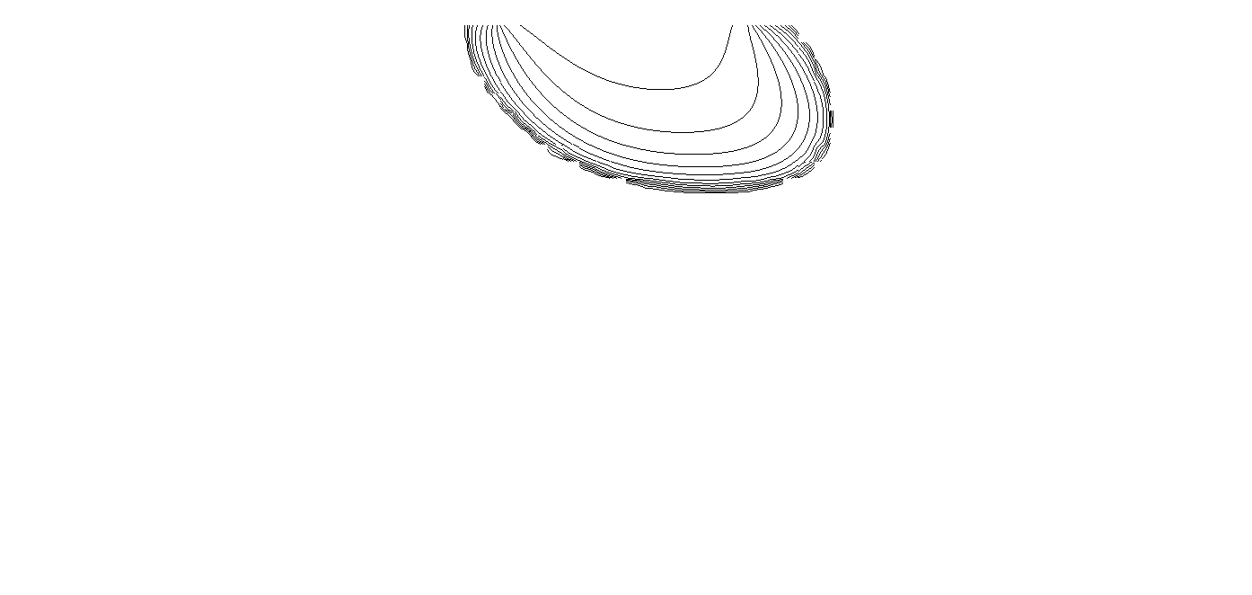
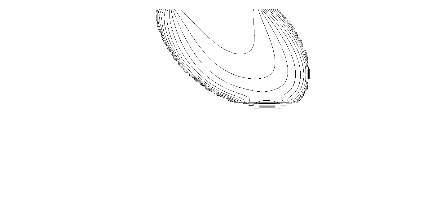
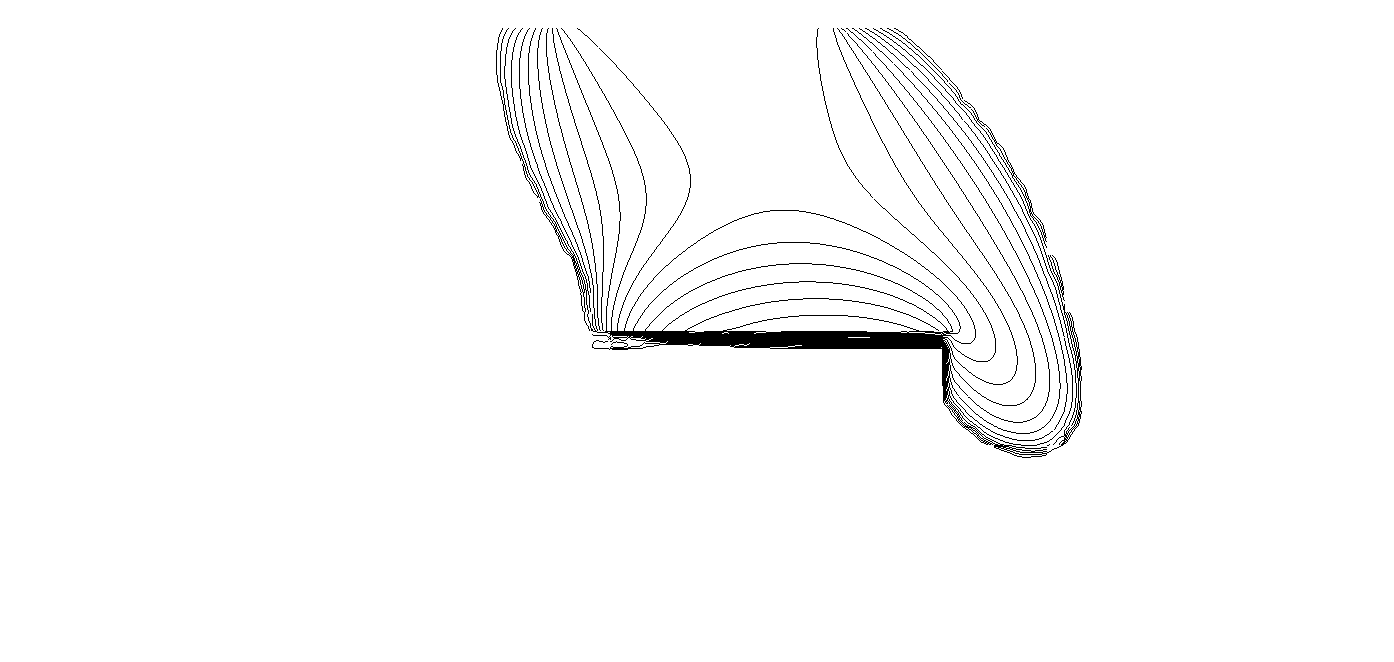
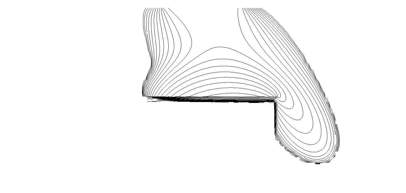
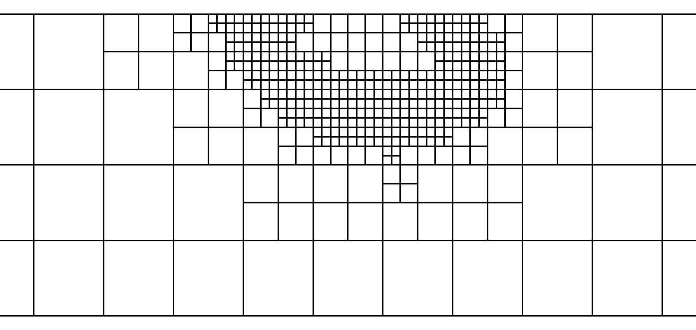
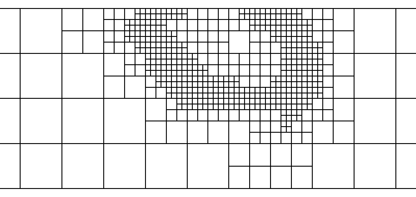
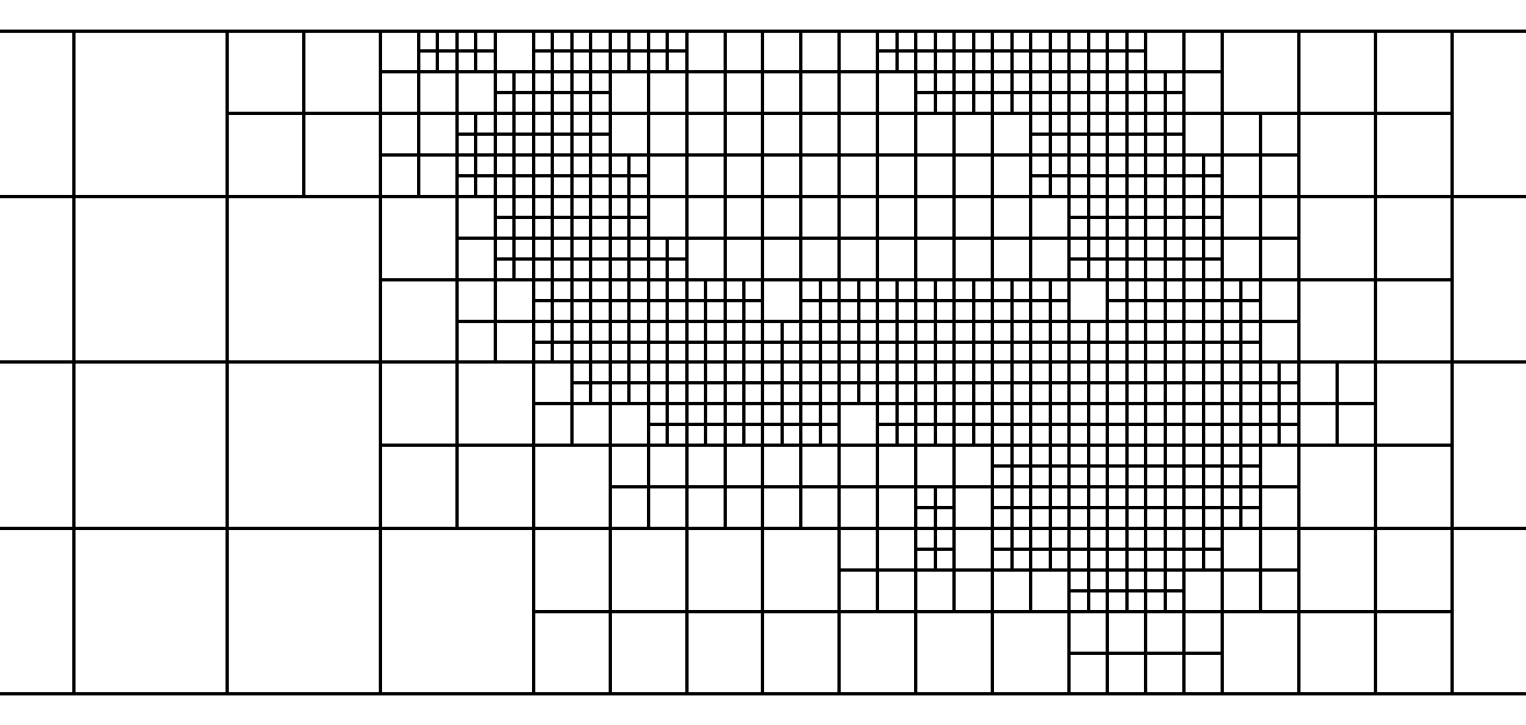
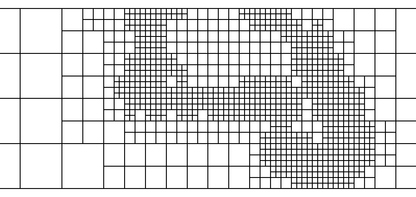
Figure 2: Evolution of the non wetting saturation $s_{n}$ at times $t=200,400,600$, and $t=800$ (top) and the corresponding adaptive grid structure (bottom).

4.2 Time step stability

In this section we compare the various splitting and solution strategy described in Section 3.2. We compare three implicit and iterative coupling schemes and two loosely coupled schemes, one of them the classical IMPES scheme.

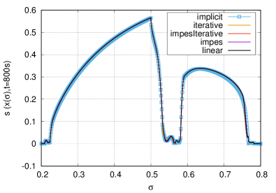
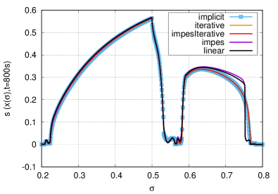
Figure 3: All schemes for $\tau=3$ (left) and $\tau=5$ (right). All schemes are able to capture the solution characteristics for times steps smaller and up to $\tau=3$. For $\tau>3$ only the fully coupled schemes are able to produce reasonable solutions, while the loosely coupled schemes do no longer capture the front position correctly.

For $\tau>3$ only the fully coupled schemes are able to produces reasonable solutions. This is illustrated in Figure 3.

In Figure 4 we compare the solution of the various fully coupled schemes for different time step sizes. If the solution converges then a correct solution profile is produced. The stability of the implicit scheme is influenced by the fact that the stabilization operator is only applied before and after the Newton solver.

In principle the explicit coupling schemes work fine for small time steps and fail to produce a valid solution for larger time steps. Here, the implicit schemes show their strength allowing for faster computation once the time step is chosen sufficiently large.

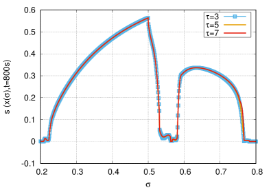
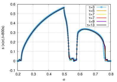
Figure 4: Left, the solution for fully coupled implicit scheme for $\tau=3,5,7$. Right the solution for the IMPES-iterative scheme for $\tau=3,5,7,9,11,13$.

4.3 Cut off stabilization

In this section we study a very simple stabilization approach aining at finding a replacement for the more complicated scaling limiter described in Section 3.4. The idea is to simply replace values for the saturation $s$ below a given threshold $s_{min}$ and $s_{max}$. Values of the saturation outside of the region considered physical will cause problems when computing the capillary pressure. So in this approach we use a very simple cut off for guaranteeing that no non negative values are used in the power laws required for the capillary pressure by replacing $s_{w,e},s_{n,e}$ by $\min\{\max\{s_{w,e},\epsilon\},1-\epsilon\}$ and $\min\{\max\{s_{w,e},\epsilon\},1-\epsilon\}$, respectively, where $\epsilon=10^{-5}$.

This approach can be directly incorporated into the symbolic description of the model as shown in C.1.

As can be clearly seen in Figure 5 significant over and undershoots are produced by all methods at the fronts. Both IMPES type splitting schemes fail to converge even for smaller time steps and the fully coupled implicit scheme produces wrong flow speeds even for moderate values of $\tau$. Only the iterative scheme manages to produce at least a reasonable representation of the flow.

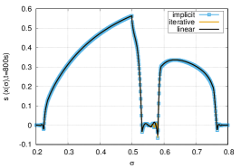
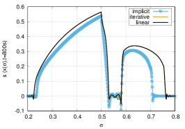
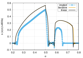
Figure 5: Left results for $\tau=1$, middle $\tau=3$ and right $\tau=5$. The IMPES and impesIterative scheme fail to converge with this approach. The other schemes all produce oscillations around the front. Interestingly, the fully coupled implicit also fails to compute the correct front position for increasing times steps.

4.4 Different model: Model B

In this section we compare our original model formulation with a description where the two-phase flow problem is modeled as a system of equations with two unknowns $\bar{p}$ and $s_{n}$. Here $\bar{p}=p_{w}+\frac{1}{2}p_{c}$:

$$-\nabla\cdot\biggl{(}(\lambda_{w}+\lambda_{n})\mathbb{K}\nabla\bar{p}+\frac{(\lambda_{n}-\lambda_{w})}{2}p_{c}^{\prime}\mathbb{K}\nabla s_{n}-(\rho_{w}\lambda_{w}+\rho_{n}\lambda_{n})\mathbb{K}\mathbf{g}\biggr{)} =q_{w}+q_{n}\ \mbox{on}\ \Omega\times(0,T),$$ (36)

$$\phi\frac{\partial s_{n}}{\partial t}-\nabla\cdot\biggl{(}\lambda_{n}\mathbb{K}(\nabla\bar{p}-\rho_{n}\mathbf{g})\biggr{)}-\frac{1}{2}\nabla\cdot\biggl{(}\lambda_{n}p^{\prime}_{c}\mathbb{K}\nabla s_{n}\biggr{)} =q_{n}\qquad\ \mbox{on}\ \Omega\times(0,T).$$ (37)

To complete the system, we add appropriate boundary and initial conditions.

$$\bar{p}(\cdot,0) =p^{0}_{w}(\cdot)+\frac{1}{2}p_{c}(s^{0}_{n}(\cdot))~{},\qquad s_{n}(\cdot,0) =s^{0}_{n}(\cdot)~{},\qquad \ \Omega,$$ in

$$\bar{p} =p_{w,D}+\frac{1}{2}p_{c}(s_{D})~{},\qquad s_{n} =s_{D}~{},\qquad \ \Gamma^{D}\times(0,T),$$ on

$$\mathbf{v}_{\alpha}\cdot\nu =J_{\alpha}~{},\qquad J_{t} =\sum_{\alpha\in\{w,n\}}J_{\alpha}~{},\qquad \ \Gamma^{N}\times(0,T).$$ on

Here, $J_{\alpha}\in\mathbb{R}$, $\alpha\in\{w,n\}$ is the inflow, $s^{0}_{n},\ p^{0}_{w},\ s_{D}$, and $\ p_{w,D}$ are real numbers.

Following the general description of the problem given in Section 2 we have $p=\bar{p},s=s_{n}$ and

$$A_{pp}(s) =(\lambda_{n}(s)+\lambda_{w}(s))\mathbb{K}~{},\qquad A_{ps}(s) =\frac{\lambda_{n}(s)-\lambda_{w}(s)}{2}p^{\prime}_{c}(s)\mathbb{K},$$

$$A_{sp}(s) =\lambda_{n}(s)\mathbb{K}~{},\qquad A_{ss}(s) =\frac{\lambda_{n}(s)}{2}p^{\prime}_{c}(s)\mathbb{K},$$

$$G_{s}(s) =0, G_{p}(s) =-(\rho_{w}\lambda_{w}(s)+\rho_{n}\lambda_{n}(s))\mathbb{K}\mathbf{g},$$

$$P_{g} =\rho_{n}\mathbf{g},$$

$$q_{p} =q_{w}+q_{n}, q_{s} =q_{n}.$$

The required changes to the Python code are again minimal and described in the C.2.

In the following we investigate the stability of the different methods with respect to the time step size when applied to modelB. We perform the same investigation described in the previous section where we used modelA. The results are summarized in Figure 6. We only investigated the stability of the three methods implicit,iterative, and impes-iterative. For modelB the splitting introduced in the impes type approach failed even for $\tau=1$ while the other two methods produce results in line with the results produced with modelA although for higher values of $\tau$ the iterative methods produce a discontenuety at the right most front as can be seen in the plots on the bottom row of Figure 6. For $\tau>5$ the implicit method fails, making modelB a less stable choice for this scheme. On the other hand the iterative approach produced results also for larger time steps $\tau=9,11,13,15$ (not shown here) but in each case the solution showed the same type of discontinuety.

Taking all the approaches into account, it is clear that modelA is the more stable representation of the problem. But our results also indicate that the stability of the iterative scheme does not seem to depend so much on the choice of the model (at the least for the two versions tested) and produces very similar results in both cases.

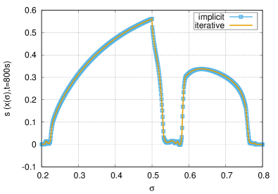
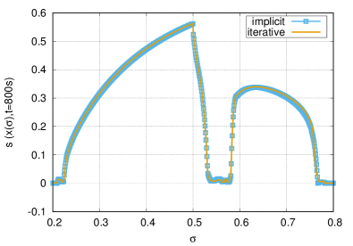
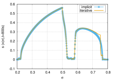
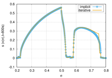
Figure 6: Results using modelB. Top row: $\tau=1,3$, bottom row: $\tau=5,7$.

4.5 P-adaptivity

Here we compare different approaches for the indicator used to set the local polynomial degree. In the following we always use the implicit method with $\tau=5$, h-adaptivity with a maximum level of three and also a maximum level of three for the polynomial order. In addition to the approach used previously we test a version without p-adaptivity and an indicator based on determining the smoothness of the solution. In regions where the indicator detects a reduction in smoothness the polynomial order is reduced but only if the grid has been refined to the maximum allowed level. The smoothness indicator is based on $\varsigma_{E}=\frac{\eta_{E}^{r}}{\eta_{E}^{r-1}}$ and we set $ptol=1$:

Algorithm 3 p-adapt: markpFrac

1:Let $\varsigma_{E}$ be given

2:for all $E\in\mathcal{T}_{h}$ do

3:     $r_{E}\mathrel{\mathop{\mathchar 58\relax}}=poldeg(E)$

4:    if $\varsigma_{E}\textless 0.01\times ptol$  then

5:       if $r_{E}\textless maxpoldeg$  then

6:          $r_{E}^{new}\mathrel{\mathop{\mathchar 58\relax}}=r_{E}+1$

7:       else

8:          $r_{E}^{new}\mathrel{\mathop{\mathchar 58\relax}}=r_{E}$

9:       end if

10:    else if $\varsigma_{E}\textgreater ptol$  then

11:       if $r_{E}\textgreater 1$  then

12:          $r_{E}^{new}\mathrel{\mathop{\mathchar 58\relax}}=r_{E}-1$

13:       else

14:          $r_{E}^{new}\mathrel{\mathop{\mathchar 58\relax}}=r_{E}$

15:       end if

16:    else

17:       $r_{E}^{new}\mathrel{\mathop{\mathchar 58\relax}}=r_{E}$

18:    end if

19:end for

The changes to the code are described in C.3.

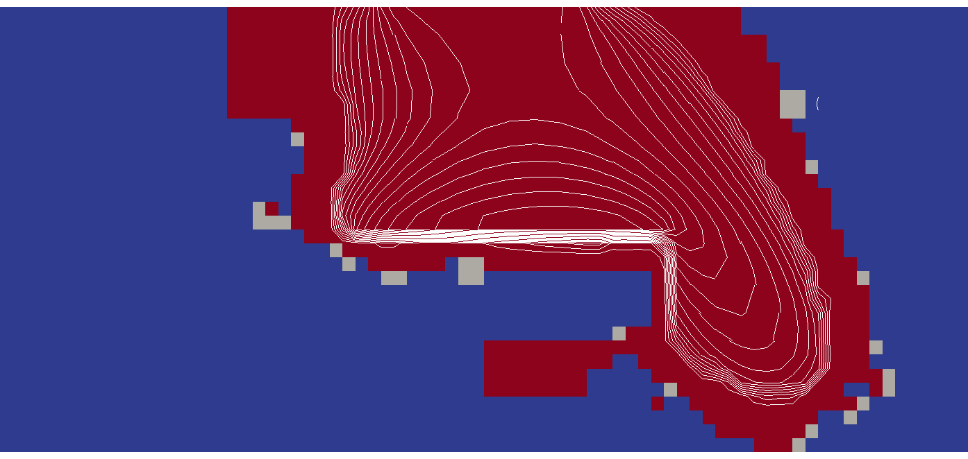
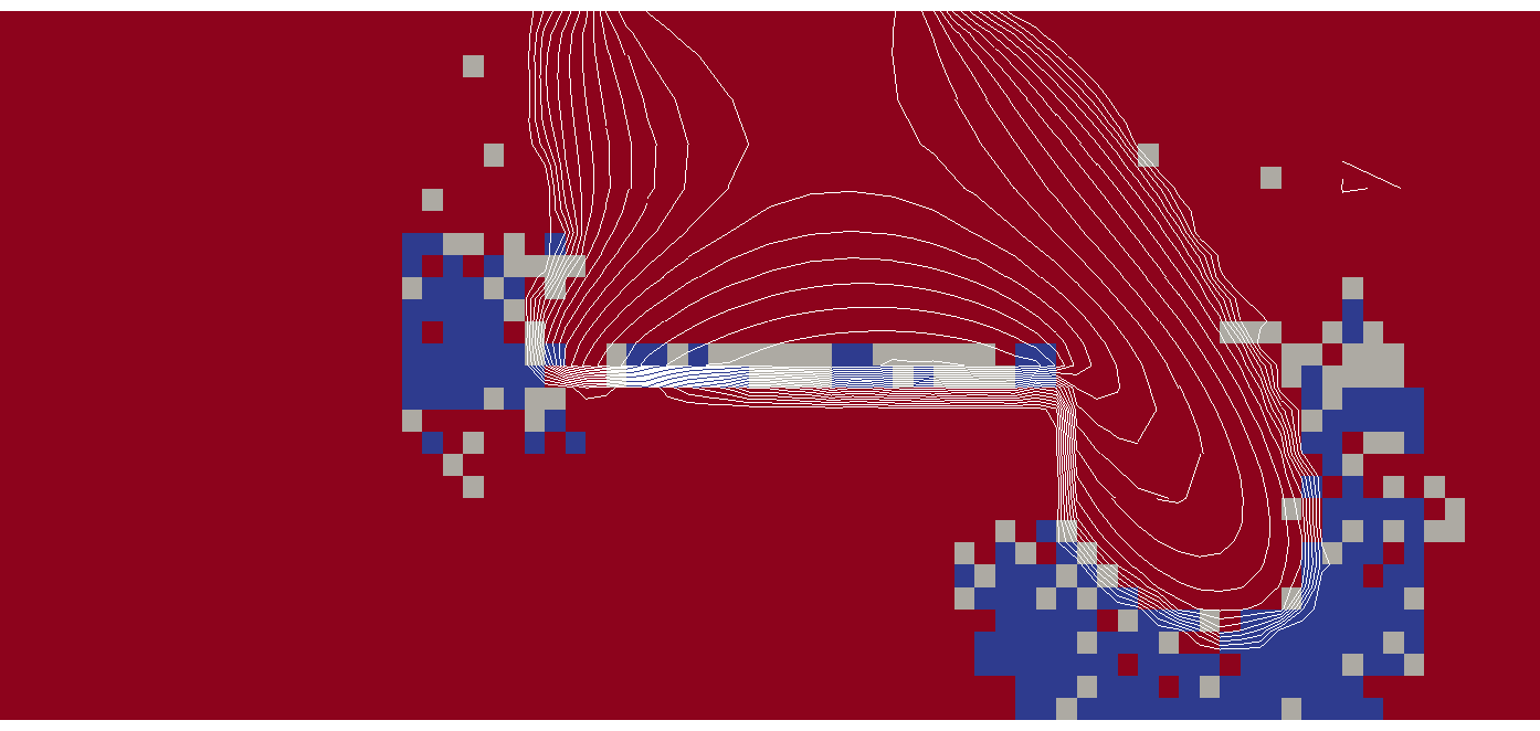
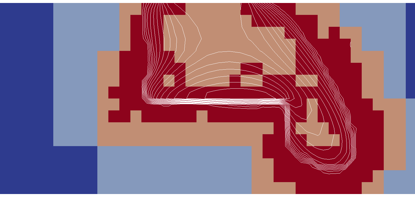
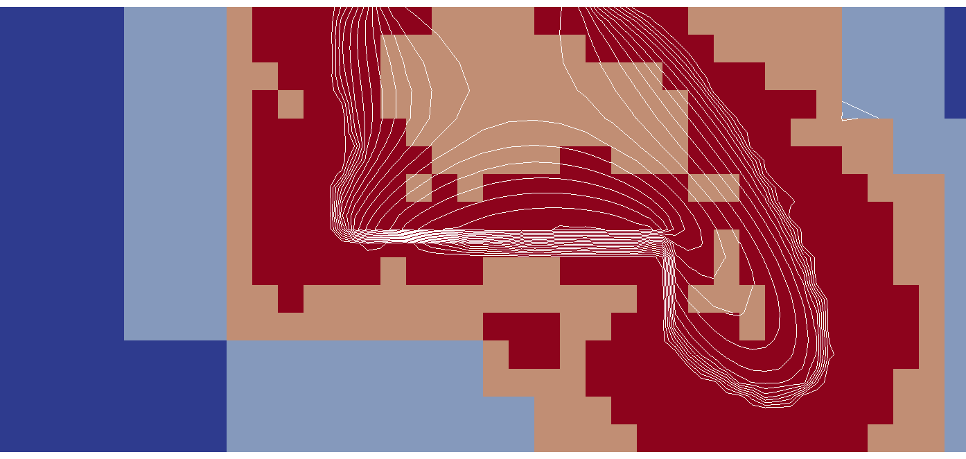
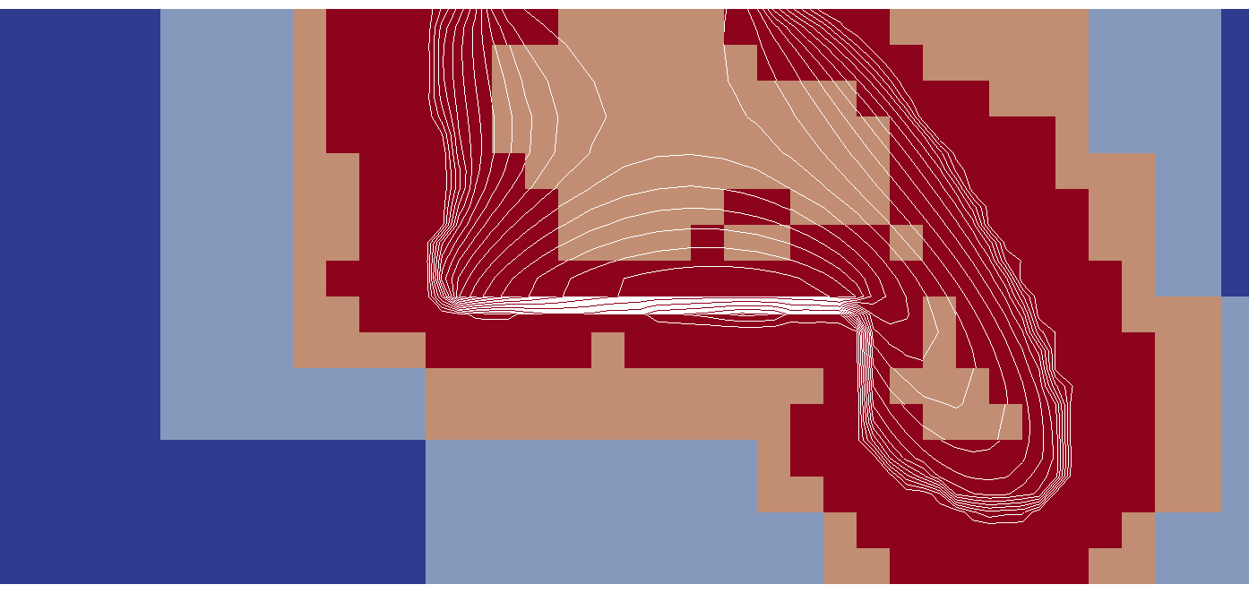
Figure 7: Comparison of different approaches for choosing the local polynomial degree. The top row shows the distribution of the polynomial order (left: original approach, right: modified indicator). Red color refers to $r=3$ and blue refers to $r=1$. The bottom row shows the grid level used for the three simulation. Red refers to $l=3$ and blue refers to $l=0$. Left to right: original approach, modified indicator, with uniform polynomial degree of three. White lines show 20 contour levels between $s_{n}=0$ and $s_{n}=0.55$.

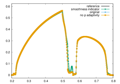
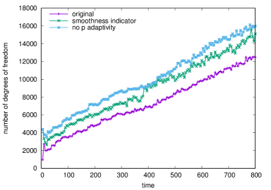
Figure 8: Comparison of different approaches for choosing the local polynomial degree. Shown $s_{n}$ over the line in equation (35).

Figure 7 shows the distribution of the polynomial order for the two p-adaptive approaches. The local grid adaptivity is of course also influenced by the choice of indicator for the polynomial degree because the values of the residuals change. This can also be seen in Figure 7. As expected for the approach discussed in Section 3.3 the polynomial order is reduced to the smallest admissible value ($r=1$) in the regions where $s_{n}$ is constant. The approach based on the smoothness indicator described in this section clearly leads to a reduction in the polynomial order at the interface of the plume. This is expected since here the solution can be said to have lower regularity. This demonstrates that the indicator works as expected. On the left in Figure 8 the solution for the different approaches along the same line given in equation (35) is shown. While the solution for the original adaptive method and the solution without adaptivity are indistinguishable, the solution with the smoothness indicator given above shows clearly an increase in numerical diffusion at the interfaces - especially at the entry point to the lens which also leads to an increase within the lens. The number of degrees of freedom during the course of the simulation depends on the number of elements and the local distribution of the polynomial degree used. The number of elements increases in time and so does the number of degrees of freedom. The right plot in Figure 8 shows the number of degrees of freedom as a function of time. Clearly the method with maximal polynomial degree on all elements requires the most degrees of freedom. Using the original indicator of p-adaptivity reduces the number of degrees of freedom to about $66\%$ at the beginning of the simulation and still to $75\%$ at the final time. The smoothness indicator given in this section only leads to a reduction of $20\%$ at the beginning of the simulation and by only $6\%$ at the final time.

Overall the indicator described in Section 3.3 does seem to lead to a better distribution of the polynomial degree with negligible influence of the actual solution. As can be seen from Figure 7, there is only little reduction of the order in the actual plume and the intermediate order $p=2$ is hardly used anywhere in the domain. Both these observations indicate that further research into p-adaptivity for this type of problem is required.

4.6 Isotropic Flow over a weak Lens

In the final section we just study a second test case. The setup is the same as in the previous example but the permeability tensors is isotropic and the lens is weaker:

$$\mathbb{K}_{\Omega\backslash\Omega_{lens}} =\begin{pmatrix}10^{-10}&0\\ 0&10^{-10}\end{pmatrix}m^{2}~{}, \mathbb{K}_{\Omega_{lens}} =\begin{pmatrix}10^{-12}&0\\ 0&10^{-12}\end{pmatrix}m^{2}~{}.$$

On the Python side the problem class the definition of $K$ has to be modified accordingly as shown in C.4.

Snapshots of the evolution of the resulting flow are shown in Figure 9. The symmetry is clearly visible both in the solution and in the grid refinement. The grid is locally refined at the interface and around the lens once the flow reaches that point. Dune to the weaker lens flow also passes through the lens. Overall our tests indicate that the conclusions obtained from our previous tests also apply to this setting.

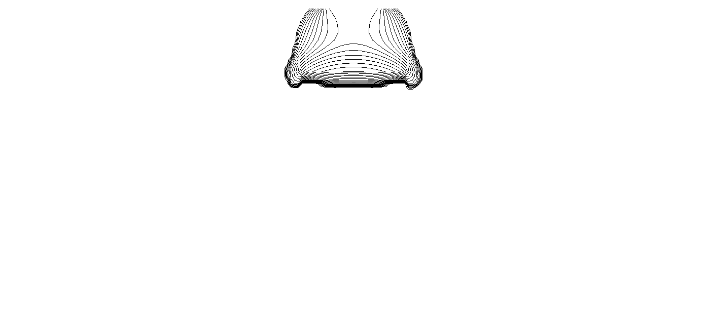
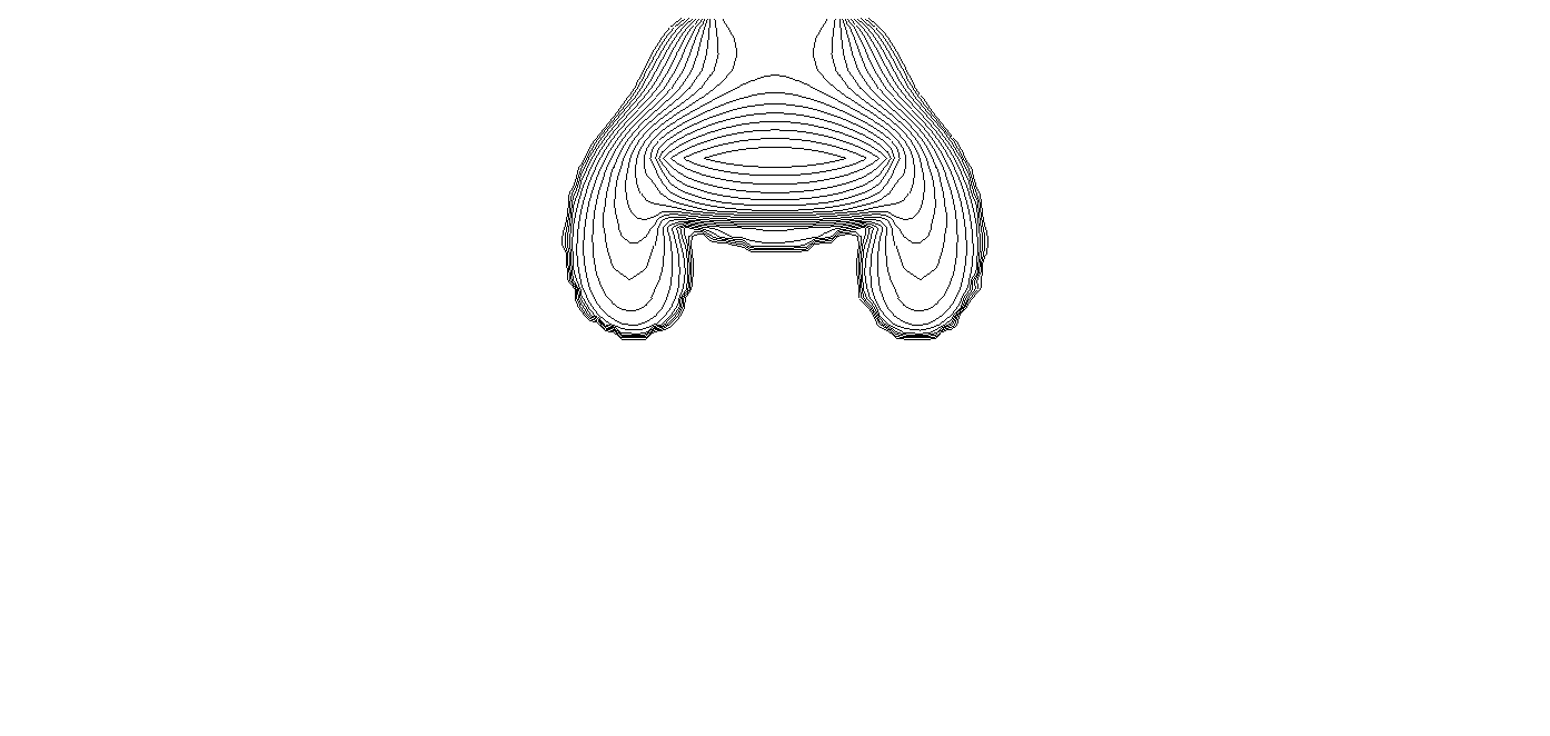
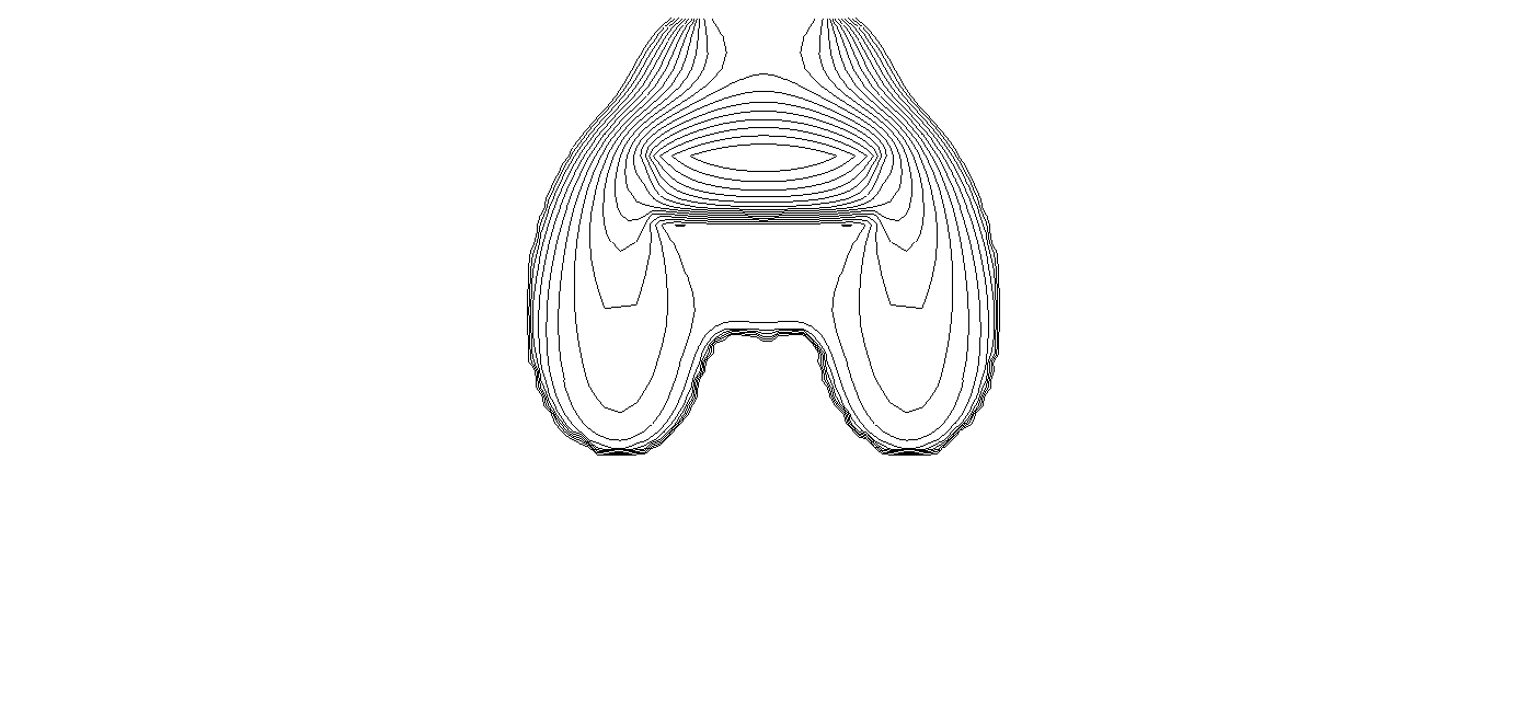
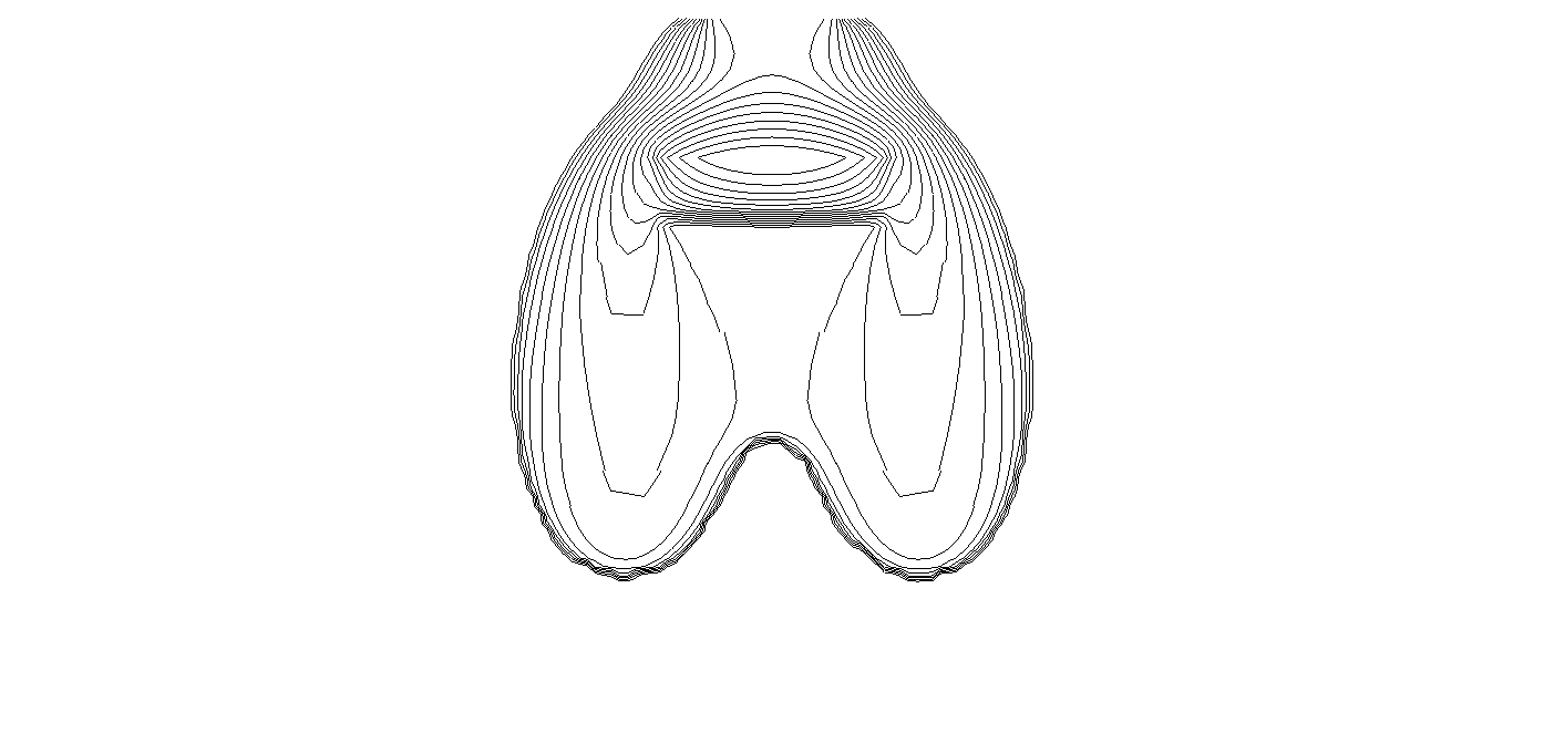
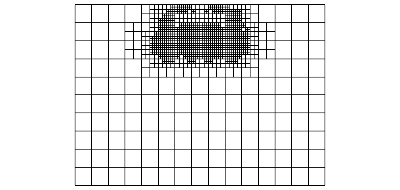
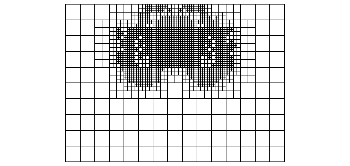
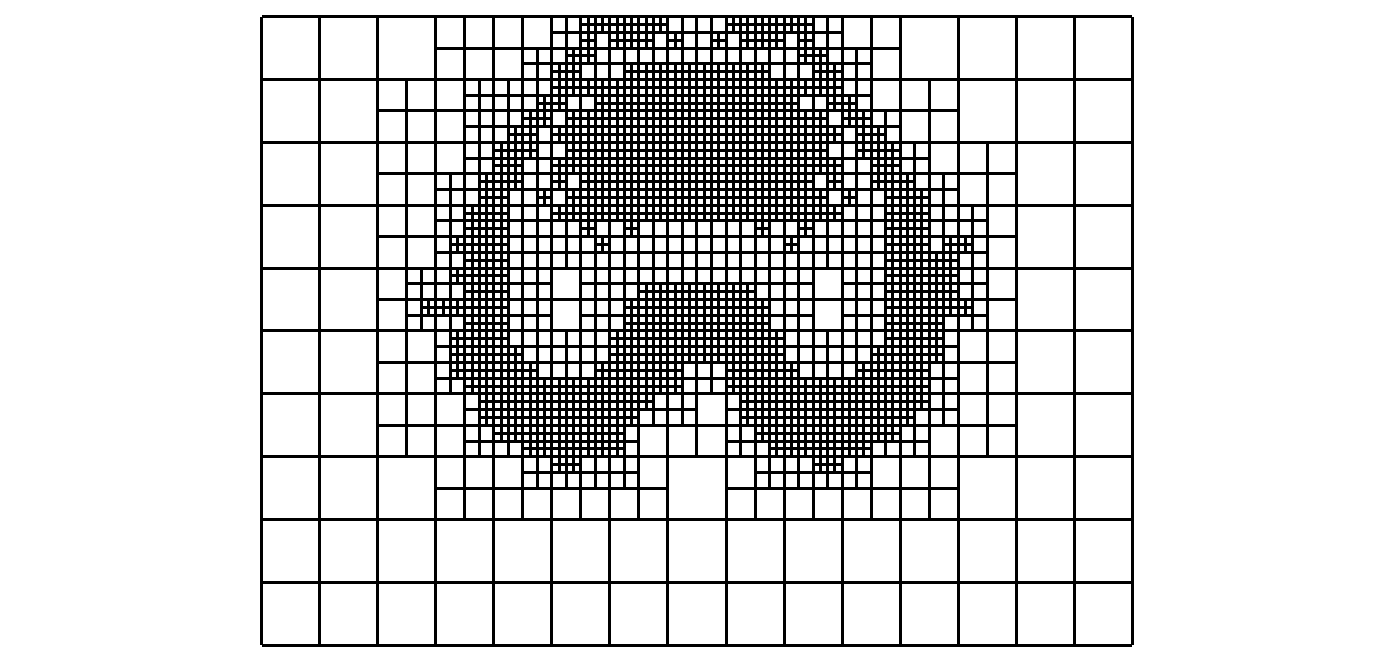
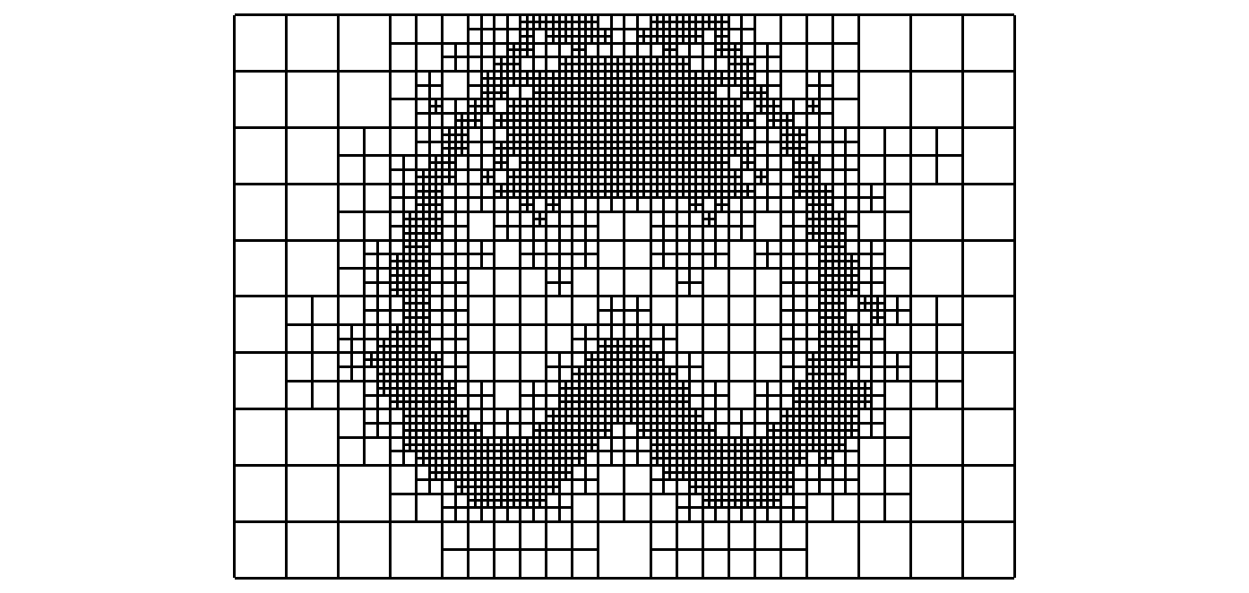
Figure 9: Evolution of the non wetting saturation $s_{n}$ for the isotropic weak lens setting at times $t=800,1600,2400$, and $t=3200$ (top) and the corresponding adaptive grid structure (bottom).

5 Conclusion

We have presented a framework that allows to study hp-adaptive schemes for two-phase flow in porous media. The presented approach allows to easily study different adaptive strategies and time stepping algorithms. The change from one algorithm to another is easily implemented. All python based implementation is in the end forwarded to C++ based implementations to ensure performance of the applications.

Furthermore, the prototypes build on very mature implementations from the Dune community to allow for a short transition from prototypes to production codes. Parallelization and extension to 3d are straightforward with the prototype presented.

We focused in this paper mostly on the stability of different approaches for evolving the solution from one time step to the next. Our results indicate that IMPES type splitting schemes can be used when smaller time step are acceptable while for larger time steps schemes solving the fully coupled equations should be used. The simple fixed point iteration seems to work quite well and seems quite stable with respect to the algorithmic approaches and models tested. It turns out that the method does show convergence issues when too small values for the stopping tolerance are used. The Newton method has more difficulty with convergence for large time steps. This suggests a combined approach where first the iterative scheme is used to reach a reasonable starting point for the Newton solver. We tested this approach and could obtain reasonable results up to time steps of $\tau=25$ effectively tripling the maximum time steps achievable when using only the Newton scheme. In future work we will focus more on this approach.

In addition, we will investigate 3d examples and the possible extension to polyhedral cells which are widely used in industrial applications. Preliminary work has been carried out, for example, in [26]. The deployment of higher order adaptive schemes is an essential tool for capturing reactive flows for applications such as polymer injections for improved oil recovery or CO₂ sequestration. Here, improved numerical algorithms help to reduce uncertainty for predictions and thus ultimately improve decision making capabilities for involved stakeholders.

Appendix A Reproducing the Results in a Docker Container

To easily reproduce the results of this paper we provide a Docker [9] image containing the presented code in a Jupyter notebook [27] and all necessary software to run it.

Once Docker is installed, the following shell command will start the Jupyter server within a Docker container:

⬇

1docker run --rm -v dune:/dune -p 127.0.0.1:8888:8888 registry.dune-project.org/dune-fem/twophaseflow:latest

Notice that all user data will be put into and kept in the Docker volume named dune for later use. This volume should not exist prior to the first run of the above command.

Open your favorite web browser and connect to 127.0.0.1:8888 and log in; the password is dune. The notebook twophaseflow contains the code used to obtain the results in this paper.

Appendix B Main Code Structure

In this section we show parts of the python script used in the simulation. The snippets are not self contained but should provide enough information to understand the overall structure. The full code which can be used to produce the simulations in Section 4.2 is available as a jupyter notebook (see Appendix A) for details. In this section we describe parts of the code following the overall structure of Sections 2 and 3.

B.1 Model A: Wetting-phase-pressure/nonwetting-phase-saturation formulation

The model description is decomposed into two parts: this first part consists of a problem class containing a static function for the pressure law $p_{c}$, the permeability tensor $K$, boundary, and initial data, and the further constants needed to fully describe the problem:

Python code

⬇

1 class AnisotropicLens:

2 dimWorld = 2

3 x = SpatialCoordinate(triangle)

4

5 g = [0,]*dimWorld ; g[dimWorld-1] = -9.810 # [m/s^2]

6 g = as_vector(g)

7 r_w = 1000. # [Kg/m^3]

8 mu_w = 1.e-3 # [Kg/m s]

9 r_n = 1460. # [Kg/m^3]

10 mu_n = 9.e-4 # [Kg/m s]

11

12 lensDomain = conditional(abs(x[1]-0.49)<0.03,1.,0.)*\

13 conditional(abs(x[0]-0.45)<0.11,1.,0.)

14

15 lens = lambda a,b: a*lensDomain + b*(1.-lensDomain)

16

17 Kdiag = lens(6.64*1e-14, 1e-10) # [m^2]

18 Koff = lens(0,-5e-11) # [m^2]

19 K = as_matrix( [[Kdiag,Koff],[Koff,Kdiag]] )

20

21 Phi = lens(0.39, 0.40) # [-]

22 s_wr = lens(0.10, 0.12) # [-]

23 s_nr = lens(0.00, 0.00) # [-]

24 theta = lens(2.00, 2.70) # [-]

25 pd = lens(5000., 755.) # [Pa]

26

27 #### initial conditions

28 p_w0 = (0.65-x[1])*9810. # hydrostatic pressure

29 s_n0 = 0 # fully saturated

30 # boundary conditions

31 inflow = conditional(abs(x[0]-0.45)<0.06,1.,0.)*\

32 conditional(abs(x[1]-0.65)<1e-8,1.,0.)

33 J_n = -5.137*1e-5

34 J_w = 1e-20 # ufl bug?

35 dirichlet = conditional(abs(x[0])<1e-8,1.,0.) +\

36 conditional(abs(x[0]-0.9)<1e-8,1.,0.)

37 p_wD = p_w0

38 s_nD = s_n0

39

40 q_n = 0

41 q_w = 0

42

43 p_c = brooksCorey

The Brooks-Corey pressure law is given by a function taking a problem class as first argument and the value non wetting phase $s_{n}$:

Python code

⬇

1 def brooksCorey(P,s_n):

2 s_w = 1-s_n

3 s_we = (s_w-P.s_wr)/(1.-P.s_wr-P.s_nr)

4 s_ne = (s_n-P.s_nr)/(1.-P.s_wr-P.s_nr)

5 cutOff = lambda a: min_value(max_value(a,0.00001),0.99999)

6 if P.useCutOff:

7 s_we = cutOff(s_we)

8 s_ne = cutOff(s_ne)

9 kr_w = s_we**((2.+3.*P.theta)/P.theta)

10 kr_n = s_ne**2*(1.-s_we**((2.+P.theta)/P.theta))

11 p_c = P.pd*s_we**(-1./P.theta)

12 dp_c = P.pd * (-1./P.theta) * s_we**(-1./P.theta-1.) * (-1./(1.-P.s_wr-P.s_nr))

13 l_n = kr_n / P.mu_n

14 l_w = kr_w / P.mu_w

15 return p_c,dp_c,l_n,l_w

The actual PDE description requires three vector valued coefficient functions one for the solution on the new time level (u), one for the solution on the previous time level (solution_old), and one for the intermediate state $\bar{s}$ used in the iterative approaches (intermediate). The vector valued test function is v. Furthermore, $\tau,\beta$ are constants used used for the time step size, the penalty factor, respectively. These can be set dynamically during the simulation:

Python code

⬇

1 s_n = u[1]

2 s_w = 1.-s_n

3 si_n = intermediate[1]

4 si_w = 1.-si_n

5

6 p_c,dp_c,l_n,l_w = P.p_c(s_n=si_n)

7

8 p_w = u[0]

9 p_n = p_w + p_c

10 gradp_n = grad(p_w) + dp_c * grad(s_n)

11

12 velocity_n = P.K*(gradp_n-P.r_n*P.g)

13 velocity_w = P.K*(grad(p_w)-P.r_w*P.g)

14

15 #### bulk equations

16 dbulk_p = P.K*( (l_n+l_w)*grad(p_w) + l_n*dp_c*grad(s_n) )

17 dbulk_p += -P.K*( (P.r_n*l_n+P.r_w*l_w)*P.g )

18 bulk_p = P.q_w+P.q_n

19 dbulk_s = P.K*l_n*dp_c*grad(s_n)

20 dbulk_s += P.K*l_n*(grad(p_w)-P.r_n*P.g)

21 bulk_s = P.q_n

B.2 Space Discretization

Given the expressions defined previously the bulk integrals for the bilinear forms can now be easily defined (compare Section 3):

Python code

⬇

1 form_p = ( inner(dbulk_p,grad(v[0])) - bulk_p*v[0] ) * dx

2 form_s = ( inner(dbulk_s,grad(v[1])) - bulk_s*v[1] ) * dx

3 form_p += J_p * v[0] * P.inflow * ds

4 form_s += J_s * v[1] * P.inflow * ds

Next we describe the skeleton terms required for the DG formulation. We use some geometric terms defined for the skeleton of the grid and also the weighted average:

Python code

⬇

1 def sMax(a): return max_value(a(’+’), a(’-’))

2 def sMin(a): return min_value(a(’+’), a(’-’))

3 n = FacetNormal(cell)

4 hT = MaxCellEdgeLength(cell)

5 he = avg( CellVolume(cell) ) / FacetArea(cell)

6 heBnd = CellVolume(cell) / FacetArea(cell)

7 k = dot(P.K*n,n)

8 def wavg(z): return (k(’-’)*z(’+’)+k(’+’)*z(’-’))/(k(’+’)+k(’-’))

As shown in Section 3 it is straightforward to construct the required penalty and consistency terms

Python code

⬇

1 ## penalty

2 form_p = penalty_p[0]/he * jump(u[0])*jump(v[0]) * dS

3 form_s = penalty_s[0]/he * jump(u[1])*jump(v[1]) * dS

4 ## consistency

5 form_p -= inner(wavg(dBulk_p),n(’+’)) * jump(v[0]) * dS

6 form_s -= inner(wavg(dBulk_s),n(’+’)) * jump(v[1]) * dS

7

8 ##### dirichlet conditions

9 ## penalty

10 form_p += penalty_p[1]/heBnd * (u[0]-p_D) * v[0] * P.dirichlet * ds

11 form_s += penalty_s[1]/heBnd * (u[1]-s_D) * v[1] * P.dirichlet * ds

12 ## consistency

13 form_p -= inner(dBulk_p,n) * v[0] * P.dirichlet * ds

14 form_s -= inner(dBulk_s,n) * v[1] * P.dirichlet * ds

The factors for the penalty terms for the DG discretization depend on the model and are given by

Python code

⬇

1 lambdaMax = k(’+’)*k(’-’)/avg(k) # P.K[0][0] + abs(P.K[0][1]) # assuming 2d and K=[[a,b],[b,a]]

2 p_c0,dp_c0,l_n0,l_w0 = P.p_c(0.5) # is not the maximm (increases for s_n->1)

3 penalty_p = beta*lambdaMax*sMax(l_n0+l_w0)

4 penalty_s = beta*lambdaMax*sMax(l_n0*dp_c0)

5 penalty_bnd_p = beta*k*(l_n0+l_w0)

6 penalty_bnd_s = beta*k*(l_n0*dp_c0)

B.3 Time stepping

The final bilinear forms used to carry out the time stepping depend on the actual schemes used. We first need to distinguish between the three schemes linear,implicit,iterative that are based on the full coupled system and the two schemes impes,iterative-impes which are based on a decoupling of the pressure and saturation equation. In the first case the final bilinear form is simply

Python code

⬇

1 form = form_s + form_p

while in the second case we define a pair of scalar forms:

Python code

⬇

1 uflSpace1 = Space((problem.dimWorld,problem.dimWorld),1)

2 u1 = TrialFunction(uflSpace1)

3 v1 = TestFunction(uflSpace1)

4 form_p = replace(form_p, { u:as_vector([u1[0],intermediate.s[0]]),

5 v:as_vector([v1[0],0.]) } )

6 form_s = replace(form_s, { u:as_vector([solution[0],u1[0]]),

7 intermediate:as_vector([solution[0],

8 intermediate[1]]),

9 v:as_vector([0.,v1[0]]) } )

10 form = [form_p,form_s]

Finally we need to fix $\bar{s}$ i.e. intermediate according to the scheme used. In the case of the implicit scheme we have intermediate=u, for linear and impes intermediate=solution_old, while for the other two schemes intermediate is an independent function used during the iteration.

The following code demonstrates how the evolution of the solution from $t^{i}$ to $t^{i+1}$ is carried out:

Python code

⬇

1 while True:

2 intermediate.assign(solution)

3 scheme.solve(target=solution)

4 limit( solution )

5 if errorMeasure(solution,solution-intermediate)

6 break

where the stopping criteria is given by

Python code

⬇

1 def errorMeasure(w,dw):

2 rel = integrate(grid, [w[1]**2,dw[1]**2], 5)

3 tol = self.tolerance * math.sqrt(rel[0])

4 rdiff = math.sqrt(rel[1])

5 return rdiff < tol

The implementation of the iterative-impes method looks almost the same

Python code

⬇

1 while n<self.maxIterations:

2 intermediate.assign(solution)

3 limit( iterate )

4 scheme[0].solve(target=solution.p)

5 scheme[1].solve(target=solution.s)

6 limit( solution )

7 n += 1

8 if error(solution,solution-intermediate):

9 break

B.4 Stabilization

Note how we apply the limiting operator directly after the next iterate has been computed. The stabilization projection operator is available as limit( solution ).

B.5 Adaptivity

The estimator is given as a form taking vector valued solution u with a scalar test function v0. This will later be used to generate an operator taking the solution and mapping into a piece wise constant scalar space with the value $\eta_{E}$ on each element:

Python code

⬇

1 uflSpace0 = Space((P.dimWorld,P.dimWorld),1) # space for indicator (could use dimRange=3)

2 v0 = TestFunction(uflSpace0)

3

4 Rvol = P.Phi*(u[1]-solution_old[1])/tau - div(dBulk_s) - bulk_s

5 estimator = hT**2 * Rvol**2 * v0[0] * dx +\

6 he * inner(jump(dBulk_s), n(’+’))**2 * avg(v0[0]) * dS +\

7 heBnd * (J + inner(dBulk_s,n))**2 * v0[0] * P.inflow * ds +\

8 penalty_s[0]**2/he * jump(u[1])**2 * avg(v0[0]) * dS +\

9 penalty_s[1]**2/heBnd * (s_D - u[1])**2 * v0[0] * P.dirichlet * ds

and since we want to use the estimator for the fully coupled implicit problem independent of the actual time stepping approach used, we add

Python code

⬇

1 estimator = replace(estimator, {intermediate:u})

The actual grid adaptivity is then carried out by calling:

Python code

⬇

1 estimator(solution, estimate)

2 hgrid.mark(markh)

3 fem.adapt(hgrid,[solution])

where the marking function is

Python code

⬇

1hTol = 1e-16 # initial value, later tTol * dt / gridSize

2def markh(element):

3 estimateLocal = estimate.localFunction(element)

4 r = estimateLocal.evaluate(element.geometry.referenceElement.center)

5 eta = sum(r)

6 if eta > hTol and element.level < maxLevel:

7 return Marker.refine

8 elif eta < 0.01*hTol:

9 return Marker.coarsen

10 else:

11 return Marker.keep

compare Algorithm 1.

Finally the p-adaptivity requires calling

Python code

⬇

1 estimator(solution, estimate)

2 # project solution to space with p-1

3 orderreduce(solution,sol_pm1)

4 # compute estimator for p-1 space

5 estimator(sol_pm1, estimate_pm1)

6 # compute smoothness indicator and modify polynomial order

7 fem.spaceAdapt(space, markp, [solution])

where the marking function markp is given by

Python code

⬇

1 def markp(element):

2 r = estimate.localFunction(element).evaluate(center)[0]

3 r_p1 = estimate_pm1.localFunction(element).evaluate(center)[0]

4 eta = abs(r-r_p1)

5 polorder = spc.localOrder(element)

6 if eta < pTol:

7 return polorder-1 if polorder > 1 else polorder

8 elif eta > 100.*pTol:

9 return polorder+1 if polorder < maxOrder else polorder

10 else:

11 return polorder

compare Algorithm 2.

Appendix C Code Modifications

C.1 Cut off stabilization

The cut off stabilization can be easily implemented with a minor change to the function defining the capillary pressure:

Python code

⬇

1def brooksCorey(P,s_n):

2 # cut all values of s below 1e-5 and above 0.99999

3 s_w = 1-s_n

4 cutOff = lambda a: min_value(max_value(a,0.00001),0.99999)

5 s_we = cutOff( (s_w-P.s_wr)/(1.-P.s_wr-P.s_nr) )

6 s_ne = cutOff( (s_n-P.s_nr)/(1.-P.s_wr-P.s_nr) )

7 kr_w = s_we**((2.+3.*P.theta)/P.theta)

8 kr_n = s_ne**2*(1.-s_we**((2.+P.theta)/P.theta))

9 p_c = P.pd*s_we**(-1./P.theta)

10 dp_c = P.pd * (-1./P.theta) * s_we**(-1./P.theta-1.) * (-1./(1.-P.s_wr-P.s_nr))

11 l_n = kr_n / P.mu_n

12 l_w = kr_w / P.mu_w

13 return p_c,dp_c,l_n,l_w

C.2 Different model: Model B

Changing the formulation of the two phase flow model requires redefining the terms for the bulk integrals and the penalty factor for the DG stabilization. The adaptation indicators and other DG terms do not need to be touched:

Python code

⬇

1 s_n = u[1]

2 p_avg = u[0]

3 p_c,dp_c,l_n,l_w = P.p_c(intermediate[1])

4

5 dBulk_p = P.K*( (l_n+l_w)*grad(p_avg) + 0.5*(l_n-l_w)*dp_c*grad(s_n) )

6 dBulk_p += -P.K*( (P.r_n*l_n+P.r_w*l_w)*P.g )

7 bulk_p = P.q_w+P.q_n

8 dBulk_s = 0.5*P.K*l_n*dp_c*grad(s_n)

9 dBulk_s += P.K*l_n*(grad(p_avg)-P.r_n*P.g)

10 bulk_s = P.q_n

11

12 #### dg penalty factors

13 lambdaMax = k(’+’)*k(’-’)/avg(k)

14 p_c0bis,dp_c0bis,l_n0,l_w0 = P.p_c(0.5)

15 penalty_p = [beta*lambdaMax*sMax(l_n0+l_w0), beta*k*(l_n0+l_w0)]

16 penalty_s = [0.5*beta*lambdaMax*sMax(l_n0*dp_c0bis), 0.5*beta*k*(l_n0*dp_c0bis)]

C.3 P-adaptivity

To change the marking strategy for the p-adaptivity the function markp needs to be redefined:

Python code

⬇

1 def markp(element):

2 polorder = spc.localOrder(element)

3 if element.level < maxLevel: return min(polorder+1,maxOrder)

4 val = pEstimator(element,element.referenceElement.center)

5 val = [estimate.localFunction(e).evaluate(x)[0],

6 estimate_pm1.localFunction(e).evaluate(x)[0]]

7 if val[0] > val[1]:

8 return polorder-1 if polorder > 1 else polorder

9 elif val[0] < 0.01*val[1]:

10 return polorder+1 if polorder < maxOrder else polorder

11 return polorder

C.4 Isotropic Flow over weak Lens

Changing the set up of the problem requires modifying the static components of the problem class i.e. for the isotropic setting with the weaker lens we need to change permeability tensors:

Python code

⬇

1 Kdiag = Lens.lens(1e-12, 1e-10) # [m^2]

2 Koff = Lens.lens(0,0) # [m^2]

3 K = as_matrix( [[Kdiag,Koff],[Koff,Kdiag]] )

References

- Ainsworth and Rankin [2009] M. Ainsworth and R. Rankin. Constant free error bounds for nonuniform order discontinuous Galerkin finite-element approximation on locally refined meshes with hanging nodes. IMA Journal of Numerical Analysis, 2009. doi: 10.1093/imanum/drp025. URL http://dx.doi.org/10.1093/imanum/drp025.
- Alkämper et al. [2016] M. Alkämper, A. Dedner, R. Klöfkorn, and M. Nolte. The DUNE-ALUGrid Module. Archive of Numerical Software, 4(1):1–28, 2016. doi: 10.11588/ans.2016.1.23252. URL http://dx.doi.org/10.11588/ans.2016.1.23252.
- Alnæs et al. [2014] M. S. Alnæs, A. Logg, K. B. Ølgaard, M. E. Rognes, and G. N. Wells. Unified form language: A domain-specific language for weak formulations of partial differential equations. ACM Trans. Math. Softw., 40(2):9:1–9:37, 2014. URL http://dx.doi.org/10.1145/2566630.
- Bastian [1999] Peter Bastian. Numerical computation of multiphase flow in porous media. PhD thesis, habilitationsschrift Univeristät Kiel, 1999. URL https://conan.iwr.uni-heidelberg.de/data/people/peter/pdf/Bastian_habilitationthesis.pdf.
- Bastian [2014] Peter Bastian. A fully-coupled discontinuous galerkin method for two-phase flow in porous media with discontinuous capillary pressure. Computational Geosciences, 18(5):779–796, 2014. URL https://doi.org/10.1007/s10596-014-9426-y.
- Bastian and Helmig [1999] Peter Bastian and Rainer Helmig. Efficient fully-coupled solution techniques for two-phase flow in porous media: Parallel multigrid solution and large scale computations. Advances in Water Resources, 23(3):199–216, 1999. URL https://doi.org/10.1016/S0309-1708(99)00014-7.
- Becker and Rannacher [1996] Roland Becker and Rolf Rannacher. A feed-back approach to error control in finite element methods: Basic analysis and examples. In East-West J. Numer. Math. Citeseer, 1996.
- Becker and Rannacher [2001] Roland Becker and Rolf Rannacher. An optimal control approach to a posteriori error estimation in finite element methods. Acta numerica, 10:1–102, 2001.
- Boettinger [2015] C. Boettinger. An introduction to docker for reproducible research, with examples from the r environment. SIGOPS Oper. Syst. Rev., 49(1):71–79, 2015.
- Brooks and Corey [1964] Royal Harvard Brooks and Arthur Thomas Corey. Hydraulic properties of porous media and their relation to drainage design. Transactions of the ASAE, 7(1):26–0028, 1964.
- Cancès et al. [2014] Clément Cancès, Iuliu Sorin Pop, and Martin Vohralík. An a posteriori error estimate for vertex-centered finite volume discretizations of immiscible incompressible two-phase flow. Mathematics of Computation, 83(285):153–188, 2014. URL https://doi.org/10.1090/S0025-5718-2013-02723-8.
- Cheng et al. [2013] Yue Cheng, Fengyan Li, Jianxian Qiu, and Liwei Xu. Positivity-preserving DG and central DG methods for ideal MHD equations. Journal of Computational Physics, 238:255 – 280, 2013. doi: https://doi.org/10.1016/j.jcp.2012.12.019. URL http://www.sciencedirect.com/science/article/pii/S0021999112007504.
- Dedner et al. [2010] A. Dedner, R. Klöfkorn, M. Nolte, and M. Ohlberger. A Generic Interface for Parallel and Adaptive Scientific Computing: Abstraction Principles and the DUNE-FEM Module. Computing, 90(3–4):165–196, 2010. URL http://dx.doi.org/10.1007/s00607-010-0110-3.
- Dedner et al. [2017] A. Dedner, S. Girke, R. Klöfkorn, and T. Malkmus. The DUNE-FEM-DG module. Archive of Numerical Software, 5(1):21–61, 2017. URL http://dx.doi.org/10.11588/ans.2017.1.28602.
- [15] Andreas Dedner and Martin Nolte. The dune-python module. in preperation, to be submitted to Archive of Numerical Software.
- Di Pietro and Ern [2011] Daniele Antonio Di Pietro and Alexandre Ern. Mathematical aspects of discontinuous Galerkin methods, volume 69. Springer Science & Business Media, 2011.
- Epshteyn and Rivière [2007] Y. Epshteyn and B. Rivière. Fully implicit discontinuous finite element methods for two-phase flow. Appl. Numer. Math., 57(4):383–401, 2007. URL http://dx.doi.org/10.1016/j.apnum.2006.04.004.
- Epshteyn and Rivière [2009] Y. Epshteyn and B. Rivière. Analysis of discontinuous Galerkin methods for incompressible two-phase flow. J. Comput. Appl. Math., 225(2):487–509, 2009. URL http://dx.doi.org/10.1016/j.cam.2008.08.026.
- Ern et al. [2010] Alexandre Ern, Igor Mozolevski, and Luciane Schuh. Discontinuous galerkin approximation of two-phase flows in heterogeneous porous media with discontinuous capillary pressures. Computer methods in applied mechanics and engineering, 199(23):1491–1501, 2010.
- Helmig and Huber [1998] Rainer Helmig and Ralf Huber. Comparison of galerkin-type discretization techniques for two-phase flow in heterogeneous porous media. Advances in Water Resources, 21(8):697–711, 1998.
- Helmig et al. [1997] Rainer Helmig et al. Multiphase flow and transport processes in the subsurface: a contribution to the modeling of hydrosystems. Springer-Verlag, 1997.
- Kane [2017] Birane Kane. Using dune-fem for adaptive higher order discontinuous galerkin methods for strongly heterogenous two-phase flow in porous media. Archive of Numerical Software, 5(1), 2017. URL http://dx.doi.org/10.11588/ans.2017.1.28068.
- [23] Birane Kane, Robert Klöfkorn, and Andreas Dedner. Adaptive discontinuous galerkin methods for flow in porous media. In Proceedings of ENUMATH 2017, the 12th European conference on numerical mathematics and advanced applications, Voss, Norway, September 25-29, 2017, accepted for publication.
- Kane et al. [2017] Birane Kane, Robert Klöfkorn, and Christoph Gersbacher. hp–Adaptive Discontinuous Galerkin Methods for Porous Media Flow. In Clément Cancès and Pascal Omnes, editors, Finite Volumes for Complex Applications VIII - Hyperbolic, Elliptic and Parabolic Problems, pages 447–456, Cham, 2017. Springer International Publishing. URL http://dx.doi.org/10.1007/978-3-319-57394-6_47.
- Klieber and Rivière [2006] W Klieber and B Rivière. Adaptive simulations of two-phase flow by discontinuous galerkin methods. Computer methods in applied mechanics and engineering, 196(1):404–419, 2006.
- Klöfkorn et al. [2017] R. Klöfkorn, A. Kvashchuk, and M. Nolte. Comparison of linear reconstructions for second-order finite volume schemes on polyhedral grids. Computational Geosciences, pages 1–11, 2017. URL http://dx.doi.org/10.1007/s10596-017-9658-8.
- Kluyver et al. [2016] T. Kluyver, B. Ragan-Kelley, F. Pérez, B. Granger, M. Bussonier, J. Frederic, K. Kelley, J. Hamrick, J. Grout, S. Corlay, P. Ivanov, D. Avila, S. Abdalla, and C. Willing. Jupyter notebooks – a publishing format for reproducible computational workflows. In F. Loizides and B. Schmidt, editors, Positioning and Power in Academic Publishing: Players, Agents and Agendas, pages 87–90. IOS Press, 2016.
- Kvashchuk [2015] Anna Kvashchuk. A robust implicit scheme for two-phase flow in porous media. Master thesis, University of Bergen, 2015. URL http://hdl.handle.net/1956/10951.
- Sun and Wheeler [2005] Shuyu Sun and Mary F Wheeler. () Norm A Posteriori Error Estimation for Discontinuous Galerkin Approximations of Reactive Transport Problems. Journal of Scientific Computing, 22(1):501–530, 2005. URL https://doi.org/10.1007/s10915-004-4148-2.
- Van Genuchten [1980] M Th Van Genuchten. A closed-form equation for predicting the hydraulic conductivity of unsaturated soils. Soil science society of America journal, 44(5):892–898, 1980.
- Vohralík and Wheeler [2013] Martin Vohralík and Mary F Wheeler. A posteriori error estimates, stopping criteria, and adaptivity for two-phase flows. Computational Geosciences, 17(5):789–812, 2013. URL https://doi.org/10.1007/s10596-013-9356-0.
- Zhang and Shu [2010] Xiangxiong Zhang and Chi-Wang Shu. On positivity-preserving high order discontinuous Galerkin schemes for compressible Euler equations on rectangular meshes. Journal of Computational Physics, 229(23):8918 – 8934, 2010. URL https://doi.org/10.1016/j.jcp.2010.08.016.