Exo-Milankovitch Cycles II: Climates of G-dwarf Planets in Dynamically Hot Systems

Abstract

Using an energy balance model with ice sheets, we examine the climate response of an Earth-like planet orbiting a G dwarf star and experiencing large orbital and obliquity variations. We find that ice caps couple strongly to the orbital forcing, leading to extreme ice ages. In contrast with previous studies, we find that such exo-Milankovitch cycles tend to impair habitability by inducing snowball states within the habitable zone. The large amplitude changes in obliquity and eccentricity cause the ice edge, the lowest latitude extent of the ice caps, to become unstable and grow to the equator. We apply an analytical theory of the ice edge latitude to show that obliquity is the primary driver of the instability. The thermal inertia of the ice sheets and the spectral energy distribution of the G dwarf star increase the sensitivity of the model to triggering runaway glaciation. Finally, we apply a machine learning algorithm to demonstrate how this technique can be used to extend the power of climate models. This work illustrates the importance of orbital evolution for habitability in dynamically rich planetary systems. We emphasize that as potentially habitable planets are discovered around G dwarfs, we need to consider orbital dynamics.

1 Introduction

Milankovitch cycles, or orbitally-induced climate variations, are thought to influence, if not control, Earth’s ice ages (Hays et al., 1976; Imbrie & Imbrie, 1980; Raymo, 1997; Lisiecki & Raymo, 2007). This mechanism has also been proposed as an important player in the habitability of exoplanets, which may have orbital evolution very different from that of Earth (Spiegel et al., 2010; Brasser et al., 2014; Armstrong et al., 2014). In Deitrick et al. (2017) (hereafter, Paper I), we discussed much of the work that has been done to understand Milankovitch cycles, both for Earth and for exoplanets. Briefly, we review the subset of the literature most concerned with the modeling of climate.

Milutin Milanković and Wladimir Köppen supplied a plausible explanation for the orbital forcing of Earth’s ice ages: small variations in summer-time insolation at high latitudes controls whether ice sheets on the continent grow or retreat. This idea is generally accepted as at least part of the story (Hays et al., 1976; Roe, 2006; Huybers & Tziperman, 2008; Lisiecki, 2010), though the reality is somewhat more complicated because of geography, ice shelf calving, atmospheric circulation, and changes in greenhouse gases (Clark & Pollard, 1998; Abe-Ouchi et al., 2013), and some studies have challenged the role of orbital forcing entirely (Wunsch, 2004; Maslin, 2016).

Much of the controversy surrounding Milankovitch theory stems from the fact that Earth’s orbital and obliquity variations are rather small—Earth’s obliquity varies by $\sim 2.5^{\circ}$ and its eccentricity by $\sim 0.05$ (Laskar et al., 1993). For exoplanets, the role of orbital forcing may be more compelling—many exoplanets have variations that are much larger than Earth’s, and there is evidence that primordial obliquities (i.e., the obliquity after the formation stage) can be very different from Earth’s present value (Miguel & Brunini, 2010).

In this study, we are interested in how planetary habitability is affected by obliquity, eccentricity, and variations of these parameters. For example, it was proposed that, at zero obliquity, the lack of insolation at the poles of an Earth-like planet would cause the ice caps to grow uncontrollably and trigger a snowball state (Laskar et al., 1993), however, climate models demonstrated that this is not the case (Williams & Kasting, 1997). In fact, the models indicate that Earth’s climate can remain stable (and warm) at any obliquity (Williams & Kasting, 1997; Williams & Pollard, 2003; Spiegel et al., 2009) at its current solar flux.

For obliquities larger than Earth’s, the seasonality of the planet is intensified (Williams & Kasting, 1997; Williams & Pollard, 2003; Spiegel et al., 2009), i.e., mid- and high-latitudes experience extremely warm summers and extremely cold, dark winters. At obliquity $\gtrsim 55^{\circ}$, the poles begin to receive more insolation over an orbit than the equator (van Woerkom, 1953; Williams, 1975, 1993; Lissauer et al., 2012; Rose et al., 2017). In such conditions, it is possible that ice sheets form at the equator (“ice-belts”), rather than at the poles (Williams & Pollard, 2003; Rose et al., 2017), but this phenomenon appears to be sensitive to the atmospheric properties and the details of the model (Ferreira et al., 2014; Rose et al., 2017). The other important development is that high obliquity ($\gtrsim 55^{\circ}$) tends to increase the distance (from the host star) to the outer edge of the habitable zone (HZ), because the insolation distribution is more even across the surface than at low obliquity (Spiegel et al., 2009; Rose et al., 2017). The habitable zone, as we discuss it here, is the range of stellar flux at which a planet with an Earth-like atmosphere can maintain liquid water on its surface (see Kasting et al., 1993; Selsis et al., 2007; Kopparapu et al., 2013).

The effect of planet’s eccentricity, $e$, on the orbitally-averaged stellar flux, $\langle S\rangle$, can be directly calculated (Laskar et al., 1993), which results in a dependence of the form:

$$\langle S\rangle\propto(1-e^{2})^{-1/2}.$$ (1)

Thus, the insolation increases as the eccentricity increases, and some studies have indeed shown that the outer-edge of the habitable zone can increase as a result (Williams & Pollard, 2002; Dressing et al., 2010). This relationship is complicated by the fact that eccentricity can introduce a global “seasonality”—a result of the varying distance between the planet and host star over an orbit. Because of Kepler’s second law, the planet spends much of its orbit near apoastron, and if the orbit is sufficiently long period, snowball states can be triggered at these times (Bolmont et al., 2016). Thus an increase in eccentricity does not warm an Earth-like planet in all cases.

How orbital and obliquity variations (exo-Milankovitch cycles) affect habitability is only beginning to be understood. Some studies have found that increases in eccentricity can rescue a planet from a snowball state (Dressing et al., 2010; Spiegel et al., 2010). Others have shown that strong variations can affect the boundaries of the habitable zone (Armstrong et al., 2014; Way & Georgakarakos, 2017). There may be some threat to the planet in the form of water loss if the planet is near the inner edge because of periastron’s proximity to the host star during high eccentricity times (Way & Georgakarakos, 2017). Exo-Milankovitch cycles may also increase or decrease the outer edge of the habitable zone, as suggested in Armstrong et al. (2014). Forgan (2016) showed that Milankovitch cycles can be very rapid for circumbinary planets, though that study did not find them a threat to planetary habitability in the cases considered.

Though the effects of different eccentricity and obliquity values and their variations have been studied by the previously discussed works, their remains no complete synthesis of orbital evolution, obliquity evolution, and climate, including the effects of ice sheets and oceans. The majority of the aforementioned works examined only static orbits and obliquities (Williams & Kasting, 1997; Williams & Pollard, 2002, 2003; Spiegel et al., 2009; Dressing et al., 2010; Ferreira et al., 2014; Bolmont et al., 2016; Rose et al., 2017). The studies that did model climate under varying orbital conditions were limited in various ways. Spiegel et al. (2010) and Way & Georgakarakos (2017) allowed eccentricity to vary, but did not include obliquity variations. Armstrong et al. (2014) included obliquity variations in addition to orbital variations. Unfortunately, that paper contained a sign error in the obliquity equations (though the code was correct) that was propagated to Forgan (2016). The climate models used by Spiegel et al. (2010) and Forgan (2016) did not include ice sheets and the thermal inertia associated with them, and so produced climates that are potentially too warm and too stable against the snowball instability. The climate model used in Armstrong et al. (2014) included ice sheets, but the outgoing longwave radiation prescription and the lack of latitudinal heat diffusion makes that model excessively stable against snowball states, and that model did not include oceans (see Section 4.6). Spiegel et al. (2010) and Forgan (2016) included oceans only in a limited capacity: the albedo and heat capacities used are the average of land and ocean properties. This mutes the seasonal response of land and the thermal inertia of water. Way & Georgakarakos (2017) used a 3D GCM, easily the most robust model of the lot, but because that model is so computationally expensive, only a handful of simulations were run.

Here, we present the first fully coupled model of orbits, obliquities, and climates of Earth-like exoplanets. This model treats land and ocean as separate components and includes ice sheet growth and decay on land. Because the model is computationally inexpensive, thousands of coupled orbit-obliquity-climate simulations can be run in a reasonable time frame. This facilitates the exploration of broad regions of parameter space and will help in the prioritization of planet targets for characterization studies.

The purpose of this study is to examine the effect of obliquity and orbital evolution on potentially habitable planets. In Paper I, we modeled the orbit and obliquity of an Earth-mass planet, in the habitable zone of a G dwarf star, with an eccentric gas giant companion. This “dynamically hot” scenario represents an end-member case, in which the orbital evolution has a large impact on the climate of the planet, without catastrophic destruction of the planetary system. In this paper, we couple the climate model described in Section 2.1 to the orbit and obliquity model and analyze the ultimate climate state of the planet. In a number of interesting scenarios, we apply a fully-analytic climate model (Rose et al., 2017) to gain some deeper understanding of the results. Finally, we revisit the G dwarf systems from Armstrong et al. (2014) with this new climate model to update the results in that paper.

2 Methods

We use a combination of a secular orbital model (DISTORB), an N-Body model (HNBody (Rauch & Hamilton, 2002)), a secular obliquity model (DISTROT), and a one-dimensional (1D) latitudinal energy balance model (EBM) with ice-sheets. For a more detailed description of DISTORB and DISTROT, and a description of how we employ the N-Body model, see Paper I. We describe the EBM and ice-sheet model below.

2.1 Climate model

The climate model, POISE (Planetary Orbit-Influenced Simple EBM), is a one-dimensional EBM (Budyko, 1969; Sellers, 1969) based on North & Coakley (1979), with a number of modifications, foremost of which is the inclusion of a model of ice sheet growth, melting, and flow. The model is one-dimensional in $x=\sin{\phi}$, where $\phi$ is the latitude. In this fashion, latitude cells of size $dx$ will not have equal width in latitude, but will be equal in area. The general energy balance equation is:

$$\begin{aligned} C(x)\frac{\partial T}{\partial t}(x,t)-&D(x,t)\nabla^{2}T(x,t)+I(x,T,t)=S(x,t)(1-\alpha(x,T,t)),\\ \end{aligned}$$ (2)

where $C(x)$ is the heat capacity of the surface at location $x$, $T$ is the surface temperature, $t$ is time, $D$ is the coefficient of heat diffusion between latitudes (due to atmospheric circulation), $I(x,t)$ is the outgoing long-wave radiation (OLR) to space (i.e., the thermal infrared flux), $S(x,t)$ is the incident insolation (stellar flux), and $\alpha$ is the planetary albedo and represents the percent of the insolation that is reflected back into space.

Though the model lacks a true longitudinal dimension, each latitude is divided into a land portion and a water portion. The land and water have distinct heat capacities and albedos, and heat is allowed to flow between the two regions. The energy balance equation can then be separated into two equations, one equation for the water component and one for the land component:

$$\begin{aligned} C_{L}\frac{\partial T_{L}}{\partial t}-D\frac{\partial}{\partial x}(1-x^{2})\frac{\partial T_{L}}{\partial x}+&\frac{\nu}{f_{L}}(T_{L}-T_{W})+I(x,T_{L},t)\\ &=S(x,t)(1-\alpha(x,T_{L},t)),\\ \end{aligned}$$ (3)

$$\begin{aligned} C_{W}^{eff}\frac{\partial T_{W}}{\partial t}-D\frac{\partial}{\partial x}(1-x^{2})\frac{\partial T_{W}}{\partial x}+&\frac{\nu}{f_{W}}(T_{W}-T_{L})+I(x,T_{W},t)\\ &=S(x,t)(1-\alpha(x,T_{W},t)),\\ \end{aligned}$$ (4)

where we have employed the co-latitudinal component of the spherical Laplacian, $\nabla^{2}$ (the radial and longitudinal/azimuthal components vanish). The effective heat capacity of the ocean is $C_{W}^{eff}=m_{d}C_{W}$, where $m_{d}$ is an adjustable parameter representing the mixing depth of the ocean. The parameter $\nu$ is used to adjust the land-ocean heat transfer to reasonable values, and $f_{L}$ and $f_{W}$ are the fractions of each latitude cell that are land and ocean, respectively.

The insolation (or solar/stellar flux) received as a function of latitude, $\phi$, and declination of the host star, $\delta$, is calculated using the formulae of Berger (1978). Declination, $\delta$, varies over the course of the planet’s orbit for nonzero obliquity. For Earth, for example, $\delta\approx 23.5^{\circ}$ at the northern summer solstice, $\delta=0^{\circ}$ at the equinoxes, and $\delta\approx-23.5^{\circ}$ at the northern winter solstice. Because $\delta$ is a function of time (or, equivalently, orbital position), the insolation varies, and gives rise to the seasons (again, assuming the obliquity is nonzero). For latitudes and times where there is no sunrise (e.g., polar darkness during winter):

$$S(\phi,\delta)=0,$$ (5)

while for latitudes and times where there is no sunset:

$$S(\phi,\delta)=\frac{S_{\star}}{\rho^{2}}\sin{\phi}\sin{\delta},$$ (6)

and for latitudes with a normal day/night cycle:

$$S(\phi,\delta)=\frac{S_{\star}}{\pi\rho^{2}}(H_{0}\sin{\phi}\sin{\delta}+\cos{\phi}\cos{\delta}\sin{H_{0}}).$$ (7)

Here, $S_{\star}$ is the solar/stellar constant (in W m^-2), $\rho$ is the distance between the planet and host star normalized by the semi-major axis (i.e. $\rho=r/a$), and $H_{0}$ is the hour angle of the of the star at sunrise and sunset, and is defined as:

$$\cos{H_{0}}=-\tan{\phi}\tan{\delta}.$$ (8)

The declination of the star with respect to the planet’s celestial equator is a simple function of its obliquity $\varepsilon$ and its true longitude $\theta$:

$$\sin{\delta}=\sin{\varepsilon}\sin{\theta}.$$ (9)

See also Laskar et al. (1993) for a comprehensive derivation. For these formulas to apply, the true longitude should be defined as $\theta=f+\Delta^{*}$, where $f$ is the true anomaly (the angular position of the planet with respect to its periastron) and $\Delta^{*}$ is the angle between periastron and the planet’s position at its northern spring equinox, given by

$$\Delta^{*}=\varpi+\psi+180^{\circ}.$$ (10)

Above, $\varpi$ is the longitude of periastron, and $\psi$ is the precession angle. Note that we add $180^{\circ}$ because of the convention of defining $\psi$ based on the vernal point, $\vernal$, which is the position of the sun at the time of the northern spring equinox. For exoplanets, there is likely a more sensible definition, however, we adhere to the Earth conventions for the sake of consistency with past literature.

A point of clarification is in order: EBMs (at least, the models employed in this study) can be either seasonal or annual. The EBM component of POISE is a seasonal model—the variations in the insolation throughout the year/orbit are resolved and the temperature of the surface at each latitude varies in response, according to the leading terms in Equations (3) and (4). In an annual model (we utilize one in this study to understand ice sheet stability; see Section 2.2), the insolation at each latitude is averaged over the year, and the energy balance equation (Eq. 2) is forced into “steady state” by setting $\partial T/\partial t$ equal to zero (this can be done numerically or analytically). By “steady state”, we mean that the surface conditions (temperature and albedo) come to final values and remain there. Seasonal EBMs, on the other hand, can be in “equilibrium”, in that the orbitally averaged surface conditions remain the same from year to year, but the surface conditions vary throughout the year.

The planetary albedo is a function of surface type (land or water), temperature, and zenith angle. For land grid cells, the albedo is:

$$\alpha=\left\{\begin{array}[]{cc}\alpha_{L}+0.08P_{2}(\sin{Z})&\begin{array}[]{c}\hskip 2.84526pt\text{if }M_{\text{ice}}=0\text{ and }T>-2^{\circ}\text{ C}\end{array}\\ \alpha_{i}&\begin{array}[]{c}\hskip 2.84526pt\text{if }M_{\text{ice}}>0\text{ or }T<=-2^{\circ}\text{ C},\end{array}\\ \end{array}\right.$$ (11)

while for water grid cells it is:

$$\alpha=\left\{\begin{array}[]{cc}\alpha_{W}+0.08P_{2}(\sin{Z})&\hskip 2.84526pt\text{if }T>-2^{\circ}\text{ C}\\ \alpha_{i}&\hskip 11.38109pt\text{if }T<=-2^{\circ}\text{ C},\\ \end{array}\right.$$ (12)

where $Z$ is the zenith angle of the sun at noon and $P_{2}(x)=1/2(3x^{2}-1)$ (the second Legendre polynomial). This last quantity is used to approximate the additional reflectivity seen at shallow incidence angles, e.g. at high latitudes on Earth. The zenith angle at each latitude is given by

$$Z=|\phi-\delta|.$$ (13)

The albedos, $\alpha_{L}$, $\alpha_{W}$ (see Table 1), not accounting for zenith angle effects, are chosen to match Earth data (North & Coakley, 1979) and account, over the large scale, for clouds, various surface types, and water waves. Additionally, the factor of $0.08$ in Equations (11) and (12) is chosen to reproduce the albedo distribution in North & Coakley (1979). The functional form of Equations 11 and 12 is also given by North & Coakley (1979)—those authors fit Earth measurements using Fourier-Legendre series, finding that the dominant albedo term is the second order Legendre polynomial. The ice albedo, $\alpha_{i}$, is a single value that does not depend on zenith angle due to the fact that ice tends to occur at high zenith angle, so that the zenith angle is essentially already accounted for in the choice of $\alpha_{i}$. Equation (11) indicates that when there is ice on land ($M_{\text{ice}}>0$), or the temperature is below freezing, the land takes on the albedo of ice. Though there are multiple conditionals governing the albedo of the land, in practice the temperature condition is only used when ice sheets are turned off in the model, since ice begins to accumulate at $T=0^{\circ}$ C, and so is always present when $T<-2^{\circ}$ C. Equation (12) indicates a simpler relationship for the albedo over the oceans: when it is above freezing, the albedo is that of water (accounting also for zenith angle effects); when it is below freezing, the albedo is that of ice.

We take the land fraction and water fraction to be constant across all latitudes. This is roughly like having a single continent that extends from pole to pole. The effect of geography on the climate is beyond the scope of this work, which is to isolate the orbitally-induced climate variations.

Like Budyko (1969) and subsequent studies, including North & Coakley (1979), we utilize a linearization of the OLR with temperature:

$$I=A+BT,.\\$$ (14)

We adopt the values for Earth as determined by North & Coakley (1979): $A=203.3$ W m^-2 and $B=2.09$ W m^{-2 ∘}C^-1, and $T$ is the surface temperature in ^∘C. The purpose of this linearization is that it allows the coupled set of equations to be formulated as a matrix problem that can be solved using an implicit Euler scheme (Press et al., 1987) with the following form:

$$\mathscr{M}\cdot T_{n+1}=\frac{CT_{n}}{\Delta t}-A+S(1-\alpha),\\$$ (15)

where $T_{n}$ is a vector containing the current surface temperatures, $T_{n+1}$ is a vector representing the temperatures to be calculated, and $C$, $A$, $S$, and $\alpha$ are vectors containing the heat capacities, OLR offsets (Equation 14), insolation at each latitude, and albedos, respectively. The matrix $\mathscr{M}$ contains all of the information on the left-hand sides of Equations 3 and 4 related to temperature. The time-step, $\Delta t$, is chosen so that conditions do not change significantly between steps, resulting in typically 60 to 80 time-steps per orbit. The new temperature values can then be calculated by taking the dot-product of $\mathscr{M}^{-1}$ with the right-hand side of Equation 15. The large time step allowed by this integration scheme greatly speeds the climate model, allowing us to run thousands of simulation for millions of years.

The ice sheet model consists of three components: mass balance (that is, local ice accumulation and ablation), longitudinal flow across the surface, and isostatic rebound of the bedrock. Longitudinal flow ensures that the ice sheets maintain a realistic size and shape, for example, they do not grow to unrealistic heights at the poles, while bedrock rebound is necessary to accurately model ice flow.

We model ice accumulation and ablation in a similar fashion to Armstrong et al. (2014). Ice accumulates on land at a constant rate, $r_{\text{snow}}$, when temperatures are below 0^∘ C. Melting/ablation occurs when ice is present and temperatures are above 0^∘ C, according to the formula:

$$\frac{dM_{\text{ice}}}{dt}=\frac{2.3\sigma(T_{\text{freeze}}^{4}-(T+T_{\text{freeze}})^{4})}{L_{h}},$$ (16)

where $M_{\text{ice}}$ is the surface mass density of ice, $\sigma=5.67\times 10^{-8}$ W m^-2 K^-4 is the Stefan-Boltzmann constant, $L_{h}$ is latent heat of fusion of ice, $3.34\times 10^{5}$ J kg^-1 and $T_{\text{freeze}}=273.15$ K. The factor of 2.3 that appears here, though not in Armstrong et al. (2014), is added to scale the melt rate to roughly Earth values of 3 mm ^∘C^-1 day^-1 (see Braithwaite & Zhang, 2000; Lefebre et al., 2002; Huybers & Tziperman, 2008).

The ice sheets flow across the surface via deformation and sliding at the base. We use the formulation from Huybers & Tziperman (2008) to model the changes in ice height due to these effects. Bedrock depression is moderately important in this model (despite the fact that we have only one atmospheric layer and thus do not resolve elevation-based effects), because the flow rate is affected. This ultimately affects the ice sheet height—without the bedrock component, the ice sheets grow to be $\sim 10\%$ taller, but less massive (see Section 3.2). The ice flow (via Huybers & Tziperman, 2008) is:

$$\begin{aligned} \frac{\partial h}{\partial t}=\frac{\partial}{\partial y}&\left[\frac{2A_{\text{ice}}(\rho_{i}g)^{n}}{n+2}\left|\left(\frac{\partial(h+H)}{\partial y}\right)^{n-1}\right|\right.\left.\cdot\frac{\partial(h+H)}{\partial y}~{}(h+H)^{n+2}+u_{b}h\right],\\ \end{aligned}$$ (17)

where $h$ is the height of the ice, $H$ is the height of the bedrock (always negative or zero, in this case), $A_{\text{ice}}$ represents the deformability of the ice, $\rho_{i}$ is the density of ice, $g$ is the acceleration due to gravity, and $n$ is the exponent in Glen’s flow law (Glen, 1958), where $n=3$. The ice height and ice surface mass density, $M_{\text{ice}}$ are simply related via $M_{\text{ice}}=\rho_{i}h$. The first term inside the derivative represents the ice deformation; the second term is the sliding of the ice at the base. The latitudinal coordinate, $y$, is related to the radius of the planet and the latitude, $y=R\phi$, thus $\Delta y=R\Delta x(1-x^{2})^{-1/2}$. Finally, $u_{b}$, the ice velocity across the sediment, is:

$$\begin{aligned} u_{b}=&\frac{2D_{0}a_{\text{sed}}}{(m+1)b_{\text{sed}}}\left(\frac{|a_{\text{sed}}|}{2D_{0}\mu_{0}}\right)^{m}\cdot\left(1-\left[1-\frac{b_{\text{sed}}}{|a_{\text{sed}}|}\min\left(h_{s},\frac{|a_{\text{sed}}|}{b_{\text{sed}}}\right)\right]^{m+1}\right),\end{aligned}$$ (18)

as described by Jenson et al. (1996). The constant $D_{0}$ represents a reference deformation rate for the sediment, $\mu_{0}$ is the reference viscosity of the sediment, $h_{s}$ is the depth of the sediment, and $m=1.25$. The shear stress from the ice on the sediment is:

$$a_{\text{sed}}=\rho_{i}gh\frac{\partial(h+H)}{\partial y},$$ (19)

and the rate of increase of shear strength with depth is:

$$b_{\text{sed}}=(\rho_{s}-\rho_{w})g\tan{\phi_{s}},$$ (20)

where $\rho_{s}$ and $\rho_{w}$ are the density of the sediment and water, respectively, and $\phi_{s}$ is the internal deformation angle of the sediment. We adopt the same numerical values as Huybers & Tziperman (2008) for all parameters related to ice and sediment (see Table 2), with a few exceptions. We use a value of $A_{\text{ice}}$ (ice deformability) that is consistent with ice at 270 K (Paterson, 1994), and a value of $r_{\text{snow}}$ (the precipitation rate) that best allows us to reproduce Milankovitch cycles on Earth (see Section 3). Note also that the value of $D_{0}$ in Table A2 of Huybers & Tziperman (2008) appears to be improperly converted for the units listed (the correct value, from Jenson et al. (1996), is listed in the text, however). With Equations (18) and (19), Equation (17) can be treated numerically as a diffusion equation, with the form:

$$\frac{\partial h}{\partial t}=D_{\text{ice}}\frac{\partial^{2}(h+H)}{\partial y^{2}},\\$$ (21)

where,

$$\begin{aligned} D_{\text{ice}}&=\frac{2A_{\text{ice}}(\rho_{i}g)^{n}}{n+2}\left|\left(\frac{\partial(h+H)}{\partial y}\right)^{n-1}\right|~{}(h+H)^{n+2}\\ &+\frac{2D_{0}\rho_{i}gh^{2}}{(m+1)b_{\text{sed}}}\left(\frac{|a_{\text{sed}}|}{2D_{0}\mu_{0}}\right)^{m}\cdot\left(1-\left[1-\frac{b_{\text{sed}}}{|a_{\text{sed}}|}\min\left(h_{s},\frac{|a_{\text{sed}}|}{b_{\text{sed}}}\right)\right]^{m+1}\right),\end{aligned}$$ (22)

and $D_{\text{ice}}$ is evaluated at each time-step, at every boundary to provide mass continuity. We solve the diffusion equation numerically using a Crank-Nicolson scheme (Crank et al., 1947).

The bedrock depresses and rebounds locally in response to the changing weight of ice above, always seeking isostatic equilibrium. The equation governing the bedrock height, $H$, is (Clark & Pollard, 1998; Huybers & Tziperman, 2008):

$$\frac{\partial H}{\partial t}=\frac{1}{T_{b}}\left(H_{eq}-H-\frac{\rho_{i}h}{\rho_{b}}\right),$$ (23)

where $T_{b}$ is a characteristic relaxation time scale, $H_{eq}=0$ is the ice-free equilibrium height, and $\rho_{b}$ is the bedrock density. We again adopt the values used by Huybers & Tziperman (2008) (see Table 2).

Because of the longer time-scales (years) associated with the ice sheets, the growth/melting and ice-flow equations are run asynchronously in POISE. First, the EBM (Equation 2) is run for 4-5 orbital periods, and ice accumulation and ablation is tracked over this time frame, but ice-flow (Equation 17) is ignored. The annually-averaged ice accumulation/ablation is then calculated from this time-frame and passed to the ice-flow time-step, which can be much longer (years). The EBM is then re-run periodically to update accumulation and ablation and ensure that conditions vary smoothly and continuously.

To clarify, the hierarchy of models and their time-steps is as follows:

1. The EBM (shortest time-step): run for a duration of several orbital periods with time-steps on the order of days. The model is then rerun at the end of every orbital/obliquity time-step and at user-set intervals throughout the ice-flow model.

2. The ice-flow model (middle time-step): run at the end of every orbital time-step (with time-steps of a few orbital periods), immediately after the EBM finishes. The duration of the model will follow one of two scenarios:

   1. If the orbital/obliquity time-step is sufficiently long, the EBM is rerun at user-set intervals, then the ice-flow model continues. The ice-flow model and the EBM thus alternate back-and-forth until the end of the orbit/obliquity time-step.

   2. If the orbital/obliquity time-step is shorter than the user-set interval, the ice-flow model simply runs until the end of the orbital time-step.

3. The orbital/obliquity model (longest time-step). The time-steps are set by the fastest changing variable (see Paper I) amongst those parameters.

This approach is shown schematically in Figure 1. The user-set interval discussed above must be considered carefully. The assumption is that annually-averaged climate conditions like surface temperature and albedo do not change much during the time span over which the ice-flow model runs. Hence, we choose a value that ensures that the ice-flow does not run so long that it dramatically changes the albedo without updating the temperature and ice balance (growth/ablation) via the EBM.

The initial conditions for the EBM are as follows. The first time the EBM is run, the planet has zero ice mass on land, the temperature on both land and water is set by the function

$$T_{0}=7.5^{\circ}\text{C}+(20^{\circ}\text{C})(1-2\sin^{2}{\phi}),$$ (24)

where $\phi$ is the latitude. This gives the planet a mean temperature of $\sim 14^{\circ}$ C, ranging from $\sim 28^{\circ}$ C in the tropics to $\sim-13^{\circ}$ at the poles. This is thus a “warm start” condition. The initial albedo of the surface is calculated from the initial temperatures. We then perform a “spin-up” phase, running the EBM iteratively until the mean temperature between iterations changes by $<0.1^{\circ}$ C, without running the orbit, obliquity, or ice-flow models, to bring the seasonal EBM into equilibrium at the actual stellar flux the planet receives and its actual initial obliquity. Then, every time the EBM is rerun (at the user-set interval or the end of the orbit/obliquity time-step), the initial conditions are taken from the previous EBM run (temperature distribution) and the end of the ice-flow run (albedo, ice mass).

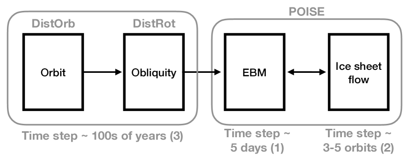
Figure 1: Hierarchy of POISE and the orbit and obliquity models. The orbit and obliquity models (DISTORB and DISTROT) are run for $\sim$ hundreds of years (with an adaptive time step determined by the rates of change of the orbital/obliquity parameters). POISE is run at the end of each orbit/obliquity time step. First, the EBM is run for several orbits, with time steps of $\sim$ 5 days. Then the ice flow model is run with time steps of $\sim 3-5$ orbits. The ice flow model runs until the next orbit/obliquity time step, or until a user-set time, at which point the EBM is rerun for several orbits.

Table 1: Parameters used in the EBM

Variable	Value	Units	Physical description
$C_{L}$	$1.55\times 10^{7}$	J m-2 K-1	land heat capacity
$C_{W}$	$4.428\times 10^{6}$	J m-2 K-1 m-1	ocean heat capacity per meter of depth
$m_{d}$	70	m	ocean mixing depth
$D$	0.58	W m-2 K-1	meridional heat diffusion coefficient
$\nu$	0.8		coefficient of land-ocean heat flux
$A$	203.3	W m-2	OLR parameter
$B$	2.09	W m-2 K-1	OLR parameter
$\alpha_{L}$	0.363		albedo of land
$\alpha_{W}$	0.263		albedo of water
$\alpha_{i}$	0.6		albedo of ice
$f_{L}$	0.34		fraction of latitude cell occupied by land
$f_{W}$	0.66		fraction of latitude cell occupied by water

Table 2: Parameters used in the ice sheet model

Variable	Value	Units	Physical description
$T_{freeze}$	273.15	K	freezing point of water
$L_{h}$	$3.34\times 10^{5}$	J kg-1	latent heat of fusion of water
$r_{\text{snow}}$	$2.25\times 10^{-5}$	kg m-2 s-1	snow/ice deposition rate
$A_{\text{ice}}$	$2.3\times 10^{-24}$	Pa-3 s-1	deformability of ice
$n$	3		exponent of Glen’s flow law
$\rho_{i}$	916.7	kg m-3	density of ice
$\rho_{s}$	2390	kg m-3	density of saturated sediment
$\rho_{w}$	1000	kg m-3	density of liquid water
$D_{0}$	$7.9\times 10^{-7}$	s-1	reference sediment deformation rate
$\mu_{0}$	$3\times 10^{9}$	Pa s	reference sediment viscosity
$m$	1.25		exponent in sediment stress-strain relation
$h_{s}$	10	m	sediment depth
$\phi_{s}$	22	degrees	internal deformation angle of sediment
$T_{b}$	5000	years	bedrock depression/ rebound timescale
$\rho_{b}$	3370	kg m-3	bedrock density

2.2 Analytical solution for ice stability

To better understand the snowball instability, we compare our results to the analytical EBM from Rose et al. (2017). Their model is an annual EBM and is analytic in that the solution is algebraic, rather than numerical. While this model does not capture seasonal variations or the thermal inertia associated with ice sheets, it is nonetheless instructive for understanding how the snowball state is triggered. We utilize the Python code developed by those authors for our results in Section 4.3.

According to the “slope-stability theorem” (Cahalan & North, 1979), the ice edge is stable as long as

$$\frac{dq}{dx_{s}}>0,$$ (25)

where $x_{s}=\sin{\phi_{s}}$, $\phi_{s}$ is the latitude of the ice edge (land and ocean are not separate component in the analytic model), and $q$ is the non-dimensional quantity

$$q=\frac{a_{0}Q}{A+BT_{\text{ref}}}.$$ (26)

The quantity $q$ represents the absorbed solar/stellar radiation, divided by the planet’s cooling function (or outgoing longwave radiation) at some temperature. Thus, it is analogous to the total heating that the planet receives, both from the host star and its own greenhouse effect. Here, $Q$ is the global average incoming flux ($4Q$ is the solar/stellar constant, $S_{\star}$) and $T_{\text{ref}}$ is the temperature threshold at which the planetary albedo switches from a value appropriate for ice free to ice covered ($T_{\text{ref}}$ is the freezing point, in other words). For ice free latitudes, the co-albedo, $a_{0}$, is a single value in the annual model. In our comparison using our seasonal model, we take this to be the average co-albedo of the unfrozen surfaces, $a_{0}=f_{L}(1-\alpha_{L})+f_{W}(1-\alpha_{W})$, and we set $T_{\text{ref}}=-2^{\circ}$ C.

Equation (25) applies to low obliquity planets. If the planet has high obliquity, ice will tend to form at the equator, and the stability condition is

$$\frac{dq}{dx_{s}}>0.$$ (27)

In the annual model, there is a distinct boundary between “low” and “high” obliquity, and the transition occurs at

$$\varepsilon=\sin^{-1}\left(\sqrt{\frac{2}{3}}\right)\approx 54.74^{\circ}.$$ (28)

See Equation (3b) of Rose et al. (2017). This angle is the obliquity at which the average annual insolation is the same at all latitudes.

At a single value of $q$, there can be multiple equilibrium locations for the ice edge—but only some of these “branches” are stable (those with positive or zero slopes) according to the slope-stability theorem. At Earth’s obliquity, the slope (Equation 25) is negative at high latitudes, which gives rise to the “small ice cap instability” (SICI), and near the equator, giving rise to the “large ice cap instability” (LICI). The slope is positive between $\sim 35^{\circ}$ and $\sim 80^{\circ}$—in other words, an ice cap extending to this range of latitudes is stable.

As we will show, this stability concept is useful in understanding how the snowball states occur in many of our simulations. However, because the seasonal EBM (POISE) is not an equilibrium model, it does deviate from the annual model at times. Hence, the ice stability diagrams that we analyze in Section 4.3 do not always accurately predict the occurrence of snowball states.

2.3 Statistics and machine learning

To extend the predictive power and utility of the model, we calculate correlations between orbital parameters and snowball states and area of ice coverage. We then employ a machine learning algorithm to determine how often we can correctly predict the climate state of the planet considered here, given a set of orbital properties. The properties that go into this analysis are shown in Table 3. There are 10 model inputs (orbit/spin parameters) and 2 model outputs ($\delta_{\text{snow}}$ and $f_{\text{ice}}$).The fractional ice cover, $f_{\text{ice}}$, is the fractional area of the globe that is covered in ice year-round at the end of the simulation (the last orbital time-step). The other output parameter, $\delta_{\text{snow}}$, is 1 if the planet is in a snowball state at the end of the simulation and 0 if it is not. Note that $\delta_{\text{snow}}=1$ when the oceans are frozen year-round; this means that there exist circumstances in which $\delta_{\text{snow}}=1$ but $f_{\text{ice}}\neq 1$ (the land component can warm above freezing seasonally, even if the oceans are frozen). In practice, this only occurs when the ice sheet model is not used, as the ice significantly alters the thermal inertia of the land. It is usually the case that $\delta_{\text{snow}}=1$ when $f_{\text{ice}}=1$ and $\delta_{\text{snow}}=0$ when $f_{\text{ice}}<1$.

Table 3: Parameters used in statistical analysis and machine-learning algorithm

Parameter	Description
$S$	Incident stellar flux (stellar constant)
$e_{0}$	Initial eccentricity
$\Delta e$	Maximum change in eccentricity
$\langle e\rangle$	Mean eccentricity
$i_{0}$	Initial inclination
$\Delta i$	Maximum change in inclination
$\langle i\rangle$	Mean inclination
$\varepsilon_{0}$	Initial obliquity
$\Delta\varepsilon$	Maximum change in obliquity
$\langle\varepsilon\rangle$	Mean obliquity
$\delta_{\text{snow}}$	Equal to 1 in snowball state, 0 otherwise
$f_{\text{ice}}$	Fractional area permanently (year-round) covered in ice

We examine how the input features of our model (Table 3) correlate with the final climate state ($\delta_{\text{snow}}$ and $f_{\text{ice}}$) to gain insight into how the underlying physical processes influence the outcomes of our simulations. For example, if the mean eccentricity correlates with likelihood that the planet enters a snowball state, we can infer that orbital dynamical processes could influence the climate evolution. Note that we cannot and do not seek to show causal relationships in the correlation analysis, but rather identify features that may impact the climate evolution.

The relationship between any feature of our model and the final state of the simulated planet climate likely has a non-linear correlation given the inherent complexities of our coupled orbital dynamics and climate model. To characterize these correlations, we compute the simple Pearson correlation coefficient ($R$) and the maximal information coefficient (MIC; Reshef et al., 2011). Pearson’s $R$ measures the linear relationship between two variables and ranges from [-1,1] with 0 representing no linear correlation and 1 and -1 represent a perfect positive and negative linear correlation, respectively. We also compute the $p-$values associated with each correlation, which are measure of statistical significance: the $p-$value indicates that there is a $p$-percent chance that the null hypothesis produces the observed correlation $R$. A $p<0.05$ is the traditional definition of significance for when testing a single hypothesis, however, since we are testing multiple hypotheses (10 in total for each climate parameter), we set the threshold for significance to $p<0.05/10$ or $p<0.005$ (a Bonferroni correction; Dunn, 1959).

The MIC characterizes non-linear relationships between variables by estimating the maximum mutual information between two variables. Mutual information between two variables characterizes the reduction in uncertainty of one variable after observing the other (see Reshef et al., 2011). For independent variables, their mutual information is 0 as observing one does not provide any insight into the other. The MIC ranges from [0,1] where MIC $=0$ represents no relationship while MIC $=1$ represents some noiseless functional relationship of any form. The MIC depends on the estimate of the joint distribution of the two variables when computing the maximum mutual information and hence is sensitive to how the variables are binned. Following the suggestion of Reshef et al. (2011), we set the number of bins to be $N^{0.6}$ for $N$ simulations. We computed the MIC using the Python package minepy (Albanese et al., 2013) for each feature versus the final surface area of ice ($f_{\text{ice}}$) and the final climate state ($\delta_{\text{snow}}$). We also define a measurement of the non-linearity associated with each parameter:

$$\zeta_{NL}=\text{MIC}-R^{2}.$$ (29)

By subtracting out a measure of the linearity of the relationship ($R^{2}$, in this case), $\zeta_{NL}$ captures the degree to which the measured correlation is non-linear. This quantity allows us to probe how the coupling between our models impact a planet’s final climate state as opposed to direct climate scalings.

As an alternative method to estimate the correlation between various features and simulation results, we turn to a machine learning (ML) approach akin to that of Tamayo et al. (2016). The purpose of this method is to look for correlations not found by either of the previous methods. Following the procedure of that study, we use an ML algorithm to predict the results of our simulations as a function of the features of our model (Table 3). We use the scikit-learn (Pedregosa et al., 2011) implementation of the random forest algorithm (Breiman, 2001). The random forest algorithm is a particularly powerful and flexible algorithm that fits an ensemble of decision trees on numerous randomized sub-samples of the data set and averages the predictions of the decision trees to produce an accurate, low-variance prediction. The random forest algorithm has a particular advantage for our purposes in that it can compute “feature importances” as a means to estimate how the algorithm weights various inputs when producing an output. An input with a high feature importance implies that the algorithm weights that feature more heavily when making a prediction. Feature importances, $\xi_{i}$, can hence be considered as a proxy for how much that feature correlates with the predicted variable (the simulation output). The feature importances are all normalized such that they sum to 1, i.e., $\sum\xi_{i}=1$.

We cast our ML problem in two forms. First, we consider the binary classification problem in which we use a random forest classifier (RFC) to predict whether or not the simulation results in a snowball planet state, $\delta_{\text{snow}}$. Second, we consider the regression problem in which we use a random forest regressor (RFR) to predict the area fraction of the planet covered in ice, $f_{\text{ice}}$, a continuous quantity that ranges from 0 to 1. In both cases, we fit the ML algorithms with the following procedure. We divide our data set using 75% of the data for our training set in which we fit and calibrate our algorithms and the remaining 25% as the testing set used to estimate the performance of our fitted algorithms on unseen data. We fit each algorithm, a process commonly referred to as “training”, and use $k-$folds cross-validation with $k=5$ to tune the hyperparameters of our model using only the training set. After training the algorithms, we find that both the RFC and RFR algorithms generalize exceptionally well. For example, the RFC’s predictions of $\delta_{\text{snow}}$ achieve a classification accuracy of $\sim 97\%$ on the testing set. After training the models and verifying their accuracy, we extract the feature importances ($\xi_{i}$) for each algorithm as shown in Tables 5 and 6. Note that in order prevent the random forest regressor (RFR) from predicting negative values for $f_{\text{ice}}$, we instead use the value $\log_{10}{(f_{\text{ice}}+1)}$ as the model output.

2.4 Initial orbital and obliquity conditions

We model the climate of planet 2 in the dynamically evolving system, TSYS, from the previous study (Paper I), over a narrower range of rotational periods. This hypothetical system, which consists of a warm Neptune, an Earth-mass planet (planet 2), and a Jovian exterior to the HZ, allows us to test the effects on habitability of exo-Milankovitch cycles. This test system is chosen as an end-member scenario, i.e., the effect of orbital evolution on climate is maximized (without destabilizing the system). The initial orbital and spin properties are shown in Table 4. As mentioned in Paper I, the warm Neptune has almost no dynamical effect on the rest of the system. To understand the effects of orbital evolution over a range of stellar fluxes, we leave the semi-major axis fixed at $a=1.0031$ au and instead vary the luminosity of the star over the range $L_{\star}=3.6\times 10^{26}$ W to $L_{\star}=3.95\times 10^{26}$ W. This corresponds to an incident stellar flux range of $S=1304.00$ W m^-2 to $S=1395.88$ W m^-2.

Table 4: Initial conditions for TSYS

Planet	1	2	3
$m$ ($M_{\oplus}$)	18.75	1	487.81
$a$ (au)	0.1292	1.0031	3.973
$e$	0.237	0.001-0.4	0.313
$i$ (∘)	1.9894	0.001-35	0.02126
$\varpi$ (∘)	353.23	100.22	181.13
$\Omega$ (∘)	347.70	88.22	227.95
$P_{rot}$ (days)		0.65,1,1.62
$\varepsilon$ (∘)		0-90
$\psi$		281.78

The planet Kepler-62 f, discussed in the previous study, requires some additional adjustments to the climate model because of its (cooler) location in the HZ and the different stellar spectrum. It is also interesting enough to warrant its own study and so we will reserve a climate analysis of this planet for a future work.

3 Model Validation

To validate the climate model, we adjust our input parameters to reproduce Earth-like values. We use the OLR parameters, $A$ and $B$, and heat diffusion coefficient $D$ from North & Coakley (1979) and surface albedos for land, water, and ice that give us good agreement to the data used in that paper, see Table 1.

3.1 Comparison with Earth and LMDG

Like Spiegel et al. (2009), we compare our vertical heat fluxes to the Earth Radiation Budget Experiment satellite data (Barkstrom et al., 1990). In Figure 2 we show the values for the flux in (blue), flux out (red), and the difference, or net heating (orange), as a function of latitude, for the Earth, using our climate model POISE. Our model compares well with the zonally- and monthly-averaged satellite data, though it is too simple to capture all of the variations. Our model also produces sharp jumps at high latitudes because of the sudden change in albedo at freezing temperatures. For the Earth, this sudden change is not seen because of a combination of geographic variations, darkening of snow and ice, clouds, etc., which are not captured in our model.

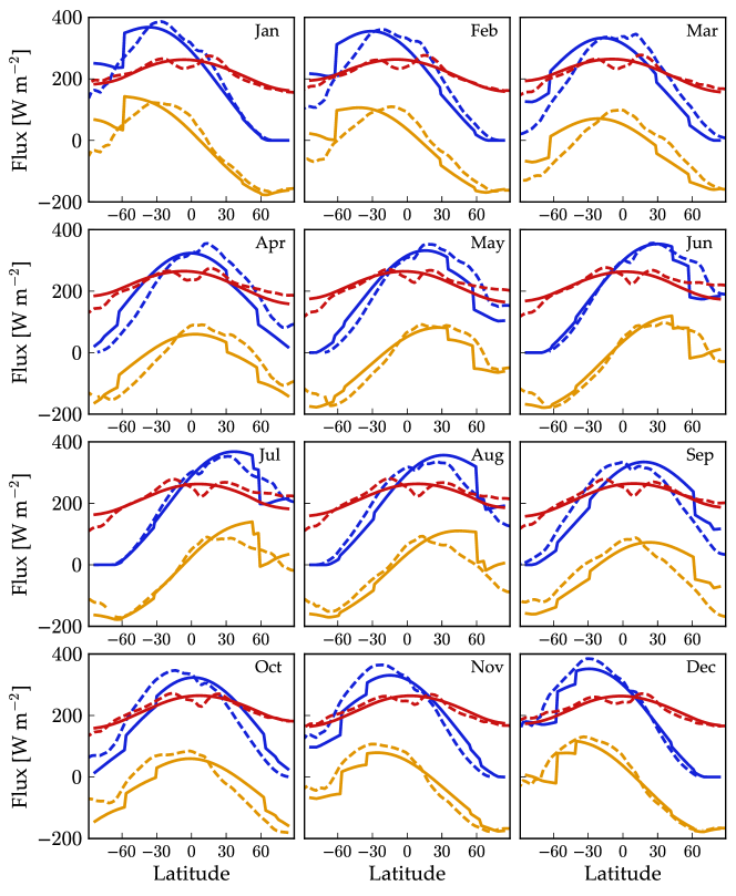
Figure 2: Monthly averaged vertical fluxes for the EBM (solid lines) and satellite data for Earth (dashed lines). Blue corresponds to incoming flux (equal to $(1-\alpha)S(\phi)$), red is the outgoing long-wave radiation (OLR), and orange is the difference (net heating).

Further, in Figures 3-4, we compare POISE to the Generic LMD 3D Global Climate Model (LMDG) (Wordsworth et al., 2011; Leconte et al., 2013a, b; Charnay et al., 2013), for rotation periods of 0.65 and 1.62 days, obliquities of 23.5^∘ and 85^∘, and eccentricities of $0.1$ and $0.3$ (eight GCM simulations in total). These initial orbital and rotational conditions sample a broad range of the conditions we explore further with the EBM. We use present Earth geography in the LMDG simulations, though in the EBM there is a fixed quantity of land at each latitude, so some difference in the models is attributable to geography. All LMDG simulations are started from an initial state corresponding to present-day Earth, with present-day topography, and run for 30 years (the typical timescale required for convergence).

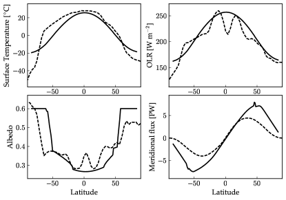
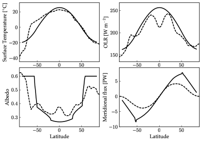
Figure 3: Comparison between our EBM (solid lines) and the LMDG 3D GCM (dashed lines), for $\varepsilon=23.5^{\circ}$, $P_{rot}=0.65$ day, and $e=0.1$ (left two columns) and $\varepsilon=23.5^{\circ}$, $P_{rot}=1.62$ day, and $e=0.1$ (right two columns). The surface temperature, OLR, and albedo compare reasonably well to the zonally-averaged quantities from LMDG considering the differences in geography and missing physics (e.g. clouds and Hadley cells). The meridional flux in the EBM peaks at $\sim 7$ PW, a bit higher than Earth’s $\sim 6$ PW, while LMDG’s peak is a tad low at $\sim 5$ PW. For $P_{rot}=1.62$ day, despite the slower rotation the meridional flux is very similar to that of the $P_{rot}=0.65$ day rotator, which suggests that parameterizations of the heat flux with rotation rate $\Omega$ ($D\propto\Omega^{-2}$; see Williams & Kasting, 1997; Spiegel et al., 2008) probably overestimate the latitudinal heat flow.

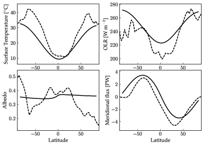
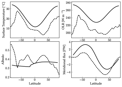
Figure 4: Same as Figure 3, but for $\varepsilon=85^{\circ}$. The left two columns again correspond to $P_{rot}=0.65$ days, the right two to $P_{rot}=1.62$ days. POISE compares worse with LMDG in these high obliquity cases. POISE captures the general patterns but underestimates the surface temperature at mid-latitudes and overestimates the OLR at the equator and south pole. At high obliquity, the geography may play a larger role than at low obliquity, due to the extreme seasonality—land and ocean have different heat capacities and so will heat on different time-scales, possibly explaining the discrepancy between the models.

In Figures 3-4 we plot the annually-averaged surface temperature, OLR, albedo, and meridional flux as a function of latitude for the POISE and LMDG simulations. With a climate model as simple as an EBM, we cannot replicate all of the variations with latitude in these quantities found by LMDG. Still, POISE captures LMDG’s general patterns in surface temperature and heat fluxes. It captures the surface temperature better in the low obliquity cases than in the high obliquity cases, though, oddly, the meridional flux in POISE matches LMDG more closely in the high obliquity cases.

A primary source of error in the high obliquity cases is that the EBM simply does not capture all of the physical processes that occur during the planet’s extreme summers. During the summer, nearly an entire hemisphere experiences sunlight for months on end, leading to extremely high temperatures and strong circulation. Ultimately, the simple parameterization of the OLR ($I=A+BT$) probably breaks down under such conditions, and convection should lead to cloud formation and a change in albedo, similar to the effect on synchronously rotating planets (Joshi, 2003; Edson et al., 2011, 2012; Yang et al., 2013).

3.2 Reproducing Milankovitch Cycles

For the purpose of this study, we tune the ice deposition rate so that the model can reproduce the Earth’s ice age cycles at $\sim 40,000$ years and $\sim 100,000$ years over a 10 million year simulation. To reproduce the effect of Earth’s moon on Earth’s obliquity, we force the precession rate to be $50.290966^{\prime\prime}$ year^-1 (Laskar et al., 1993). This choice does not perfectly match the dynamics of the Earth-moon-sun system, but it is close enough to replicate the physics of the ice age cycles. The results of this tuning are shown in Figure 5 (see Huybers & Tziperman (2008), Figure 4, for comparison), for a 200,000 year window. The ice sheets in the northern hemisphere high latitude region grow and retreat as the obliquity, eccentricity (not shown), and climate-precession-parameter, or CPP ($e\sin{(\varpi+\psi)}$), vary. The ice deposition rate is less than that used by Huybers & Tziperman (2008) and so the ice accumulation per year is slightly smaller. The ice ablation occurs primarily at the ice edge (around latitude $60^{\circ}$) and is slightly larger than Huybers & Tziperman (2008), but is qualitatively similar.

There are a number of differences between our reproduction of Milankovitch cycles and those of Huybers & Tziperman (2008). Most notably, our ice sheets tend to persist for longer periods of time, taking up to three obliquity cycles to fully retreat. We also require a lower ice deposition (snowing) rate than Huybers & Tziperman (2008) in order to ensure a response from the ice sheets to the orbital forcing. We attribute these differences primarily to the difference in energy balance models used for the atmosphere. For example, our model has a single-layer atmosphere with a parameterization of the OLR tuned to Earth, while Huybers & Tziperman (2008) used a multi-layer atmosphere with a simple radiative transfer scheme. Further, while the model Huybers & Tziperman (2008) contained only land, our model has both land and water which cover a fixed fraction of the surface. The primary effect of having an ocean in this model is to change the effective heat capacity of the surface. This dampens the seasonal cycle, and affects the ice sheet growth and retreat. Thus, our seasonal cycle is somewhat muted compared to theirs, and our ice sheets do not grow and retreat as dramatically on orbital time scales. Ultimately, our ice age cycles are more similar to the longer late-Pleistocene cycles than to $\sim 40,000$ year cycles of the early-Pleistocene.

Even though we cannot perfectly match the results of Huybers & Tziperman (2008), we are comfortable with these results for a number of reasons. First, both models make approximations to a number of physical processes and thus have numerous parameters that have to be tuned to reproduce the desired behavior. Second, both models are missing boundary conditions based on the continent distribution of the Earth—continental edges can limit the equator-ward advance of ice sheets or alter the speed of their flow through calving of ice shelves. Finally, because the purpose of this study is to understand the response of ice sheets and climate to orbital variations, it is enough to merely ensure that the ice sheets respond in a way qualitatively similar to the Earth’s without being overly sensitive (i.e., resulting in ice free or snowball conditions with an insolation value of the solar constant, $\sim 1370$ W m^-2, and an OLR prescription similar to Earth’s).

To investigate the importance of the bedrock depression/rebound component of the model, we compare this Earth case to one with $\partial H/\partial t$ (Eqn 23) set to zero. Figure 6 shows the ice sheet height, $h+H$, and surface mass density, $\Sigma_{i}$, with (upper panels) and without the bedrock component (middle panels), and the difference (lower panels). The ice sheets reach higher altitude (by several hundred meters) without bedrock depression, but the ice mass is decreased by $\sim 10^{5}$ kg m^-2. The effect of isostasy is thus to confine the ice sheets while allowing them to grow larger. While this subtly increases the thermal inertia, it ultimately makes a minor difference in the prevalence of snowball states in our results (Section 4).

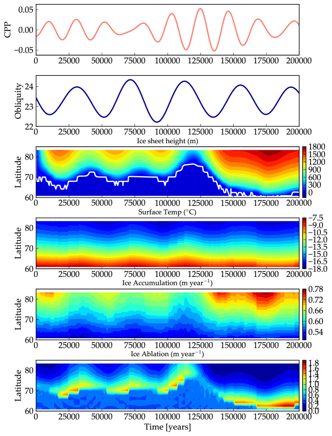
Figure 5: Milankovitch cycles on Earth, in the northern hemisphere. The panels are arranged to compare with Figure 4 of Huybers & Tziperman (2008). From top to bottom, we have: CPP $=e\sin{(\varpi+\psi)}$, obliquity, ice sheet height (m), annually averaged surface temperature (^∘C), annual ice accumulation rate (m yr^-1), and annual ice ablation rate (m yr^-1).

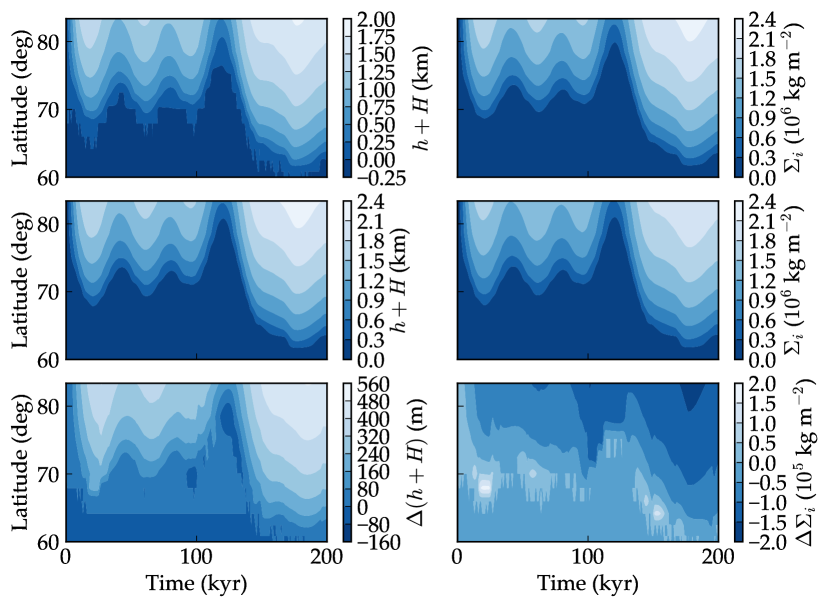
Figure 6: Ice sheet evolution for Earth with (upper panels) and without (middle panels) isostatic depression and rebound of the bedrock. Also shown is the difference (lower panels). The left panels show the ice sheet height/altitude; the right panels show the surface density of the ice. Without the bedrock model, the ice grows taller (in elevation), but there is less ice overall because the surface does not sink under the weight of the ice.

4 Results

4.1 Static cases

First, we identify the regimes in which ice sheets are able to form. The presence and distribution of permanent ice on land will depend on the stellar flux received by the planet and the planet’s obliquity. In Figure 7 we show how ice covered fraction, $f_{\text{ice}}$ depends on incoming stellar flux at two obliquities ($\varepsilon=23.5^{\circ}$ and $\varepsilon=50^{\circ}$). Note that this initial ice coverage in each simulation is determined by the initial temperature distribution (Eqn. 24), and is very different from the final result in most cases. The ice coverage includes both land and ocean grid-points. The stellar flux is normalized by Earth’s value, $S_{0}=1367.5$ W m^-2. No orbital evolution occurs in these simulations, however, the spin axis is allowed to precess at a rate set by the stellar torque (see Paper I). Two quantities are displayed in these plots: the fractional area of the planet that is permanently ice covered (i.e. ice covered year-round) and the total ice mass at the end of the simulation.

At the lowest stellar flux values, the planet is globally ice covered ($f_{\text{ice}}=1$), but the ice sheet mass remains at zero. This is because, in our model, precipitation is shut off when the oceans are frozen over, and in these coldest cases, the oceans freeze over during the spin-up phase of the simulation, thus no ice accumulates on land. In the $\varepsilon=50^{\circ}$ case, the coldest cases are actually not ice covered year round. Since the oceans have frozen before ice sheets can grow on land, and the thermal inertia of the land is low (compared to the oceans and the ice sheets), the temperature over land actually rises above freezing during the summer months. Thus, the fact that $f_{\text{ice}}<1$ is probably a side effect of our modeling choices—these cases really are in a snowball state. At higher stellar flux values, it takes hundreds to thousands of years for the planet to cool into the snowball state, thus ice sheets are allowed to grow on land. Because it takes much more energy in the model to melt a thick layer of ice (than to simply heat the land), these cases remain fully ice covered year-round.

All points within the gray-shaded region entered a snowball state in $<200$ kyr, after which all ice sheets appear to be stable under static orbital/obliquity conditions. The light-blue region corresponds to our “transition region”, wherein stable ice sheets form at some latitudes and persist year-round. In the dark-blue region, ice may form seasonally, but no permanent ice sheets appear. Note that in the $\varepsilon=23.5^{\circ}$ cases, the ice covered area is not necessarily equal to zero because the oceans remain frozen at the poles year round, even though no ice sheets grow from year to year.

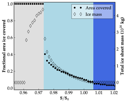
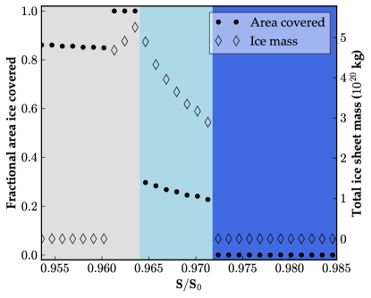
Figure 7: The fractional ice cover, $f_{\text{ice}}$, for static orbital/obliquity conditions as a function of stellar flux, $S/S_{0}$, where $S_{0}=1367.5$ W m^-2, for $\varepsilon=23.5^{\circ}$ (left) and $\varepsilon=50^{\circ}$ (right). The ice covered area includes both land and ocean grid-points. The gray shaded area represents snowball states (the ocean surface is permanently and completely ice-covered), dark-blue represent ice-free (no year-round ice) states, and light-blue is the “transition region”, where the ocean is not totally ice-covered and ice sheets form on land. For reference, the Antarctic ice sheet is estimated to be $27\times 10^{6}$ km³, on the order of $10^{19}$ kg of ice mass (Fretwell et al., 2013).

The higher obliquity case remains clement (not in a snowball state) at lower stellar flux, and thus higher semi-major axis, than the low obliquity case, consistent with past results (Spiegel et al., 2009; Armstrong et al., 2014). The transition region is also narrower in this case, and the boundary between the transition region and the ice sheet free region (light- and dark-blue) is sharper, consistent with Rose et al. (2017), which demonstrated that ice (as represented by $T<0^{\circ}$ C on land or ocean) is less stable on higher obliquity planets. Interestingly, even though the obliquity is less than $55^{\circ}$ (the approximate value at which the annual insolation at the poles begins to exceed that of the equator), the ice sheets in the transition region form along the equator, not the poles. This is a result of the temperature dependence of ice ablation—when the atmosphere is warmer, the ice melts faster (see Equation (16)). Even though the equatorial latitudes receive more sunlight over the course of an orbit, the summers are much more intense at the poles. High latitude summers are then much warmer than conditions ever get at the equator. So while the snowy season at the poles may be colder and longer, the intense summers are more than enough to melt the ice accumulated during winters, whereas the melting seasons are not hot enough or long enough to fully melt the equatorial ice.

4.2 Dynamically evolving cases

Next, we vary the initial eccentricity, inclination, rotation rate, and obliquity of planet 2 (Earth-mass) in our test system. Figures 10-15 show the fractional area of the planet that is ice covered for several slices of this parameter space at an incident stellar flux of $S=1332.27$ W m^-2, or $S/S_{0}=0.974$. This stellar flux puts the planet right at the boundary between the snowball state and the transition zone for a planet with low eccentricity and $23.5^{\circ}$ obliquity (Figure 7, left panel), and places the $\varepsilon_{0}=50^{\circ}$ simulations in the ice-free regime.

The obliquity amplitude ($\Delta\varepsilon$) is shown in each panel as contours (see Paper I). The blue-white color scale in each figure shows the fraction, $f_{\text{ice}}$, of the total area of the panel that is permanently ice-covered, where “permanent” means covered year-round as in the previous section. Thus, some cases that have $f_{\text{ice}}=0$ do have seasonal ice formation.

The left panels shows the climate conditions assuming a static orbit and obliquity fixed at the initial values. Here, inclination has no direct effect on the insolation or climate, so $f_{\text{ice}}$ depends only on the eccentricity ($S\propto(1-e^{2})^{-1/2}$). The planet is in a snowball state $f_{\text{ice}}=1$ at $e=0$, but as $e$ is increased, $f_{\text{ice}}$ decreases. The stellar torque on the equatorial bulge is included and results in a constant axial precession rate, but this has minimal impact on the total ice coverage.

In the middle panels, the orbit and obliquity are also static, but they are fixed at the mean values from the 2 Myr simulation. The structure of this phase space is very different from that of the static initial conditions (upper right). For the cases with $\varepsilon_{0}=23.5^{\circ}$ (Figures 10, 12, and 14), using the mean properties tends to decrease the portion of phase space with $f_{\text{ice}}=1$, however, for the $\varepsilon_{0}=50^{\circ}$ cases (Figures 11, 13, and 15), the mean properties produce snowball states where none existed before (at the initial values). Hence, using the mean orbital/obliquity properties in a climate simulation produces very different results from using the initial (or, perhaps, observed) properties.

Finally, the right panel in each figure shows $f_{\text{ice}}$ for the full 2 Myr simulation with evolving orbits and obliquities. Now, the ice coverage increases almost universally, and snowball states are much more frequent than under static conditions. There are some configurations that had $f_{\text{ice}}=1$ under static conditions but are not completely ice covered under evolving conditions (at low inclination and low eccentricity, for example), but in general, the evolution tends to encourage the snowball instability, except at higher $e_{0}$. Interestingly, there are several blue “islands” (where $f_{\text{ice}}<1$) that are completely surrounded by snowball states in the dynamically evolving cases. There is a complex interplay between the obliquity and eccentricity that we will discuss in more detail in Section 4.3.

Figure 8: Mean eccentricity values as a function of initial inclination and eccentricity. These values are used as input to the climate model for the middle panels of Figures 10-15. There is a single simulation in the upper right corner for which the orbital model fails (the eccentricity exceeds $\sim 0.66$)—we model the system and climate up until the code halts, but this point does not factor heavily into our analysis.

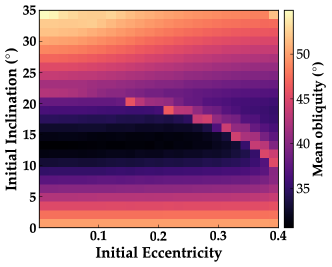
Figure 9: Mean obliquity values as a function of initial inclination and eccentricity for $P_{rot}=1$ day at $\varepsilon_{0}=23.5^{\circ}$ (left) and $\varepsilon_{0}=50^{\circ}$. These values are used in the climate model for the middle panels of Figures 10 and 11. The high obliquity “arc” through the center of each panel is the result of a secular spin-orbit resonance (see Paper I). Corresponding plots for $P_{rot}=1.62$ days and $P_{rot}=0.65$ days (that is, the conditions used in the middle panels of Figures 12-15) appear very similar in structure. The range of mean obliquity values is smaller ($15^{\circ}\lesssim\langle\varepsilon\rangle\lesssim 50^{\circ}$) for $P_{rot}=1.62$ days, while it is slightly increased ($15^{\circ}\lesssim\langle\varepsilon\rangle\lesssim 65^{\circ}$) for $P_{rot}=0.65$.

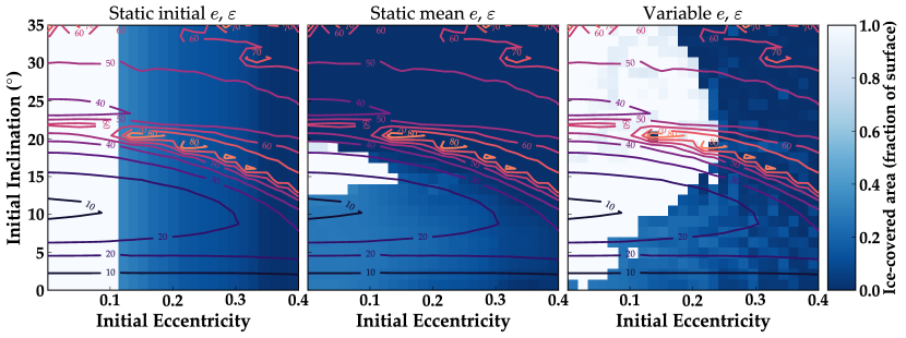
Figure 10: Climate states as a function of initial eccentricity and inclination, for $P_{rot}=1$ day and initial obliquity $\varepsilon_{0}=23.5^{\circ}$, with a stellar constant of $S=1332.27$ W m^-2. Each panel shows the fraction of the surface area that is permanently ice-covered over the final orbit (blue color-scale) and contours of $\Delta\varepsilon$ (black lines), under three different conditions: left, static orbit and obliquity at the initial values; middle, static orbit and obliquity at the mean values from the simulation; right, dynamically evolving orbit and obliquity.

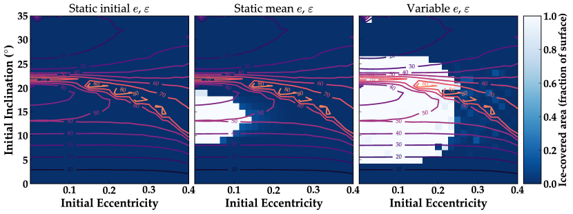
Figure 11: Same as Figure 10 but for $P_{rot}=1$ day and initial obliquity $\varepsilon_{0}=50^{\circ}$.

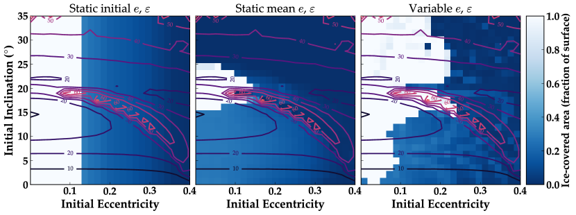
Figure 12: Same as Figure 10 but for $P_{rot}=1.62$ day and initial obliquity $\varepsilon_{0}=23.5^{\circ}$.

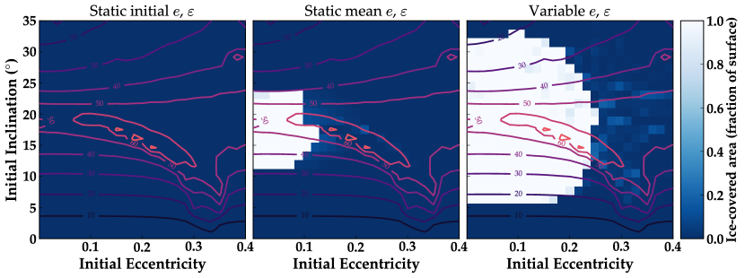
Figure 13: Same as Figure 10 but for $P_{rot}=1.62$ day and initial obliquity $\varepsilon_{0}=50^{\circ}$.

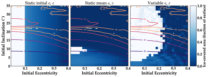
Figure 14: Same as Figure 10 but for $P_{rot}=0.65$ day and initial obliquity $\varepsilon_{0}=23.5^{\circ}$.

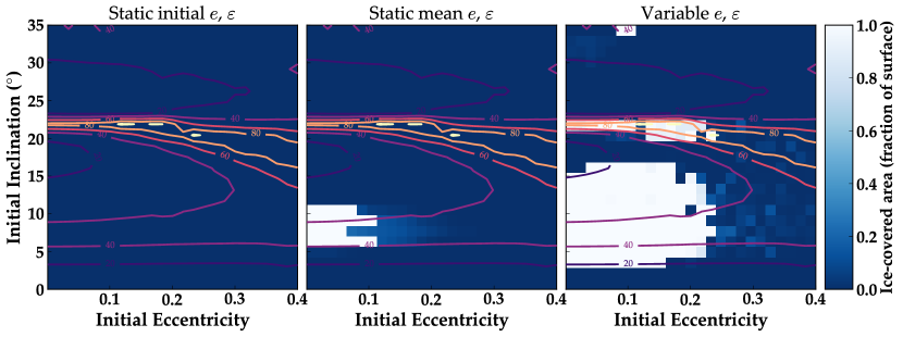
Figure 15: Same as Figure 10 but for $P_{rot}=0.65$ day and initial obliquity $\varepsilon_{0}=50^{\circ}$.

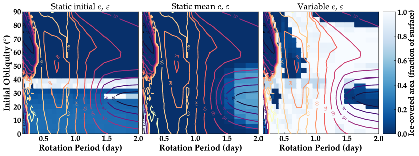
Figure 16: Same as Figure 10 but varying $P_{rot}$ and $\varepsilon$ with $e_{0}=0.2$ and $i_{0}=20^{\circ}$.

Figure 16 illustrates the effects of rotation rate and initial obliquity. The ice cover is shown in the same style as Figures 10-15, but with $e$ and $i$ fixed, and $\varepsilon_{0}$ and $P_{\text{rot}}$ varied instead. Under static initial eccentricity and obliquity (left), low obliquity cases form some permanent ice, while high obliquity cases form none. From $\varepsilon\sim 33^{\circ}-40^{\circ}$, the planet enters a snowball state, because the ice edge is unstable at these obliquities (see Section 4.3), but these cases lack the warming effect that comes with even higher obliquity. The static mean conditions do not enter a snowball state anywhere in this parameter space. With a variable orbit and obliquity, snowball states occur throughout much of this space. Note also that the obliquity variation in some regions is extremely large in amplitude and sometimes chaotic (see Paper I).

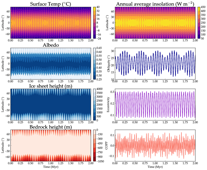
Figure 17: Evolution of climate and orbit for a case at initial values: $S=1332.27$ W m^-2, $e_{0}=0.16725$, $i_{0}=14.54^{\circ}$, $\varepsilon_{0}=23.5^{\circ}$, and $P_{rot}=1.62$ day (inside the horizontal blue strip near the center of Figure 12, right panel). The climate-obliquity-precession-parameter is defined as COPP $=e\sin{\varepsilon}\sin{(\varpi+\psi)}$ and represents the asymmetry between the northern and summer hemispheres (see text).

Figure 17 shows the climate and orbit evolution for a point in the parameter space of Figure 12 ($\varepsilon=23.5^{\circ}$ and $P_{\text{rot}}=1.62$ day). In this figure we have the surface temperature, planetary albedo, ice sheet height, bedrock height, and insolation, all averaged over an orbit or “year”, as a function of latitude and time. Also shown are the three parameters that affect the insolation: obliquity, eccentricity, and “climate-obliquity-precession-parameter” (COPP), which is defined as:

$$\text{COPP}=e\sin{\varepsilon}\sin{(\varpi+\psi)},$$ (30)

where, again, $\varpi+\psi$ represents the instantaneous angle between periastron and the planet’s position at its northern spring equinox. This is essentially the same as the commonly used “climate precession parameter” or CPP, but additionally takes into account the effect of obliquity variations (which are neglected in the CPP because Earth’s are very small). COPP can be thought of as a measurement of the asymmetry between the northern and southern hemispheres, and so varies with the angle $\varpi+\psi$, modulated by the eccentricity and obliquity. When COPP $>0$, the northern hemisphere receives more stellar flux than the southern; vice-versa for COPP $<0$.

Despite the climate in Figure 17 approaching very near to snowball states, the planet remains clement throughout this 2 Myr evolution. Ice sheets grow and recede at both poles rather dramatically, from almost nothing to nearly 4 km in height (in some regions) and back. This oscillation is a result of a nearly 200 W m^-2 swing in the annual insolation over $\sim 50,000$ years, due to the combined effects of the obliquity and eccentricity variations. The envelope of the obliquity oscillation is imprinted on the latitude of the ice edge, though the primary driver of growth and retreat is the change in eccentricity. The ice edge progresses into the mid-latitudes during periods when the obliquity oscillation is lowest in amplitude.

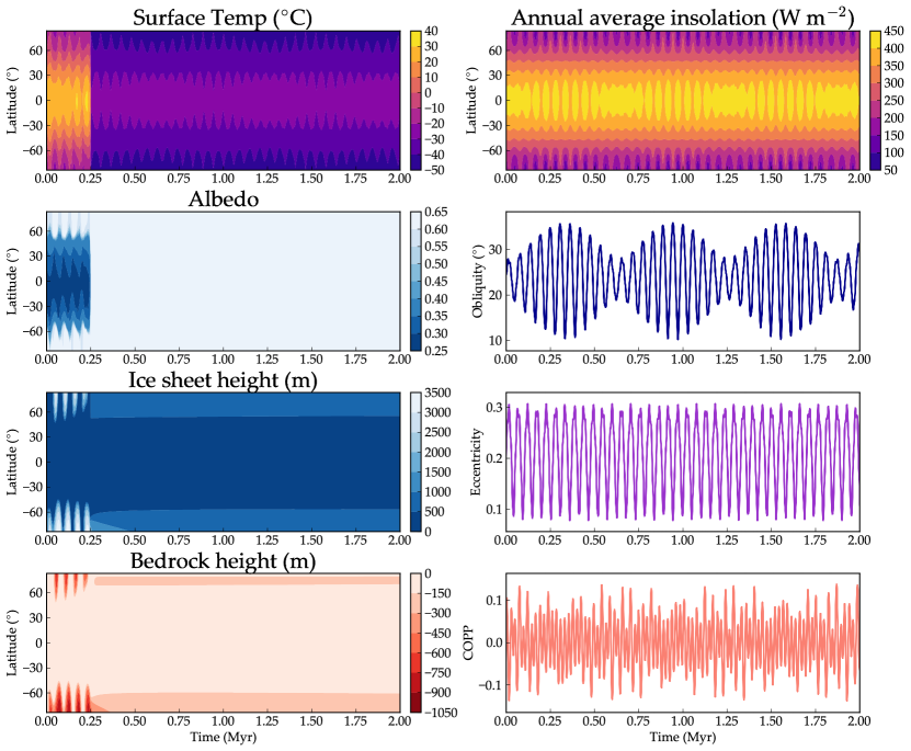
Figure 18: Same as Figure 17 but for $e_{0}=0.16725$, $i_{0}=16.04^{\circ}$, $\varepsilon_{0}=23.5^{\circ}$, and $P_{rot}=1.62$ day (slightly lower inclination than the case in that Figure). A snowball state occurs at $t\sim 750,000$ years—the temperature drops globally, the albedo approaches that of ice everywhere, and ice sheets no longer grow (precipitation is shut off artificially) and instead just gradually flatten.

In Figure 18, we have the same evolution for a case immediately adjacent to that in Figure 17. The eccentricity and obliquity variations are very similar to the previous case, however, the obliquity peaks at a slightly higher value ($\sim 35^{\circ}$, compared to $\sim 30^{\circ}$ in the previous). The ice sheets grow and retreat in a similar fashion until the obliquity approaches its highest value, at which point the planet abruptly enters a snowball state. The appearance of the large ice cap instability (LICI) is somewhat counter to expectation here—as we have shown before (and numerous other studies have found), high obliquity tends to grant a planet additional warmth at low stellar flux. The analytic solution to the annual EBM from Rose et al. (2017) provides an explanation for how the instability occurs, see Section 4.3.

In addition to snowball states, we also observe some very high temperatures at high-obliquity, high-eccentricity times. For a case with $\varepsilon_{0}=23.5^{\circ}$, $P_{rot}=1$ day, $e_{0}=0.3$, and $i_{0}=17.5^{\circ}$, which is inside the secular resonance in Figure 10, the obliquity reaches $\sim 80^{\circ}$ while the eccentricity is $\sim 0.4$. Figure 19 shows the orbital/obliquity evolution and the resulting average, minimum, and maximum surface temperatures (over an orbital period). At the highest obliquity times, the north pole of the planet reaches $140^{\circ}$ C. Such strong heating should probably result in strong convection, which would increase the albedo (due to cloud formation) and cause increased horizontal heat flow, but our simple EBM does not model such effects (see Section 3.1). Thus this temperature is improbable, except perhaps over dry continental interiors. It is beyond the scope of this study to comprehensively model this scenario with a GCM, but it is worth future investigation in the future.

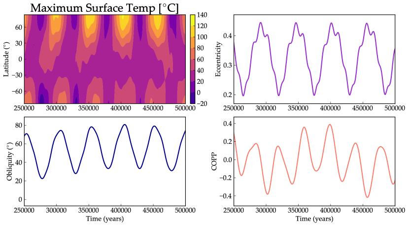
Figure 19: Evolution of the orbit, obliquity and maximum surface temperature for a case with $P_{rot}=1$ day, $\varepsilon_{0}=23.5^{\circ}$, $e_{0}=0.3$, and $i_{0}=17.5^{\circ}$ over a 250 kyr period. The upper left panel is the maximum surface temperature over an orbit (averaged over land/ocean); lower left, obliquity; upper right, eccentricity; lower right, COPP. The obliquity reaches large values because of the secular spin-orbit resonance (see Paper I). The highest obliquity times correspond to high eccentricity times. As a result, the insolation at high latitudes is extremely high during summer and the surface temperature exceeds the boiling point of water. This effect depends also on the angle $\varpi+\psi$ (the angle between the equinox and pericenter) and is responsible for the additional variation in maximum temperature between these warm periods.

4.3 Examining ice stability

In the previous section, we saw that the ice caps often become unstable as a result of the orbital/obliquity evolution. Though we highlighted the snowball instability (or LICI), the SICI can also be observed in the rapid retreat of the ice sheets. We can use the analytical solution from Rose et al. (2017) (Section 2.2) to plot the ice edge latitude as a function of the dimensionless parameter, $q$ (Figure 20). As we discussed, the slope of this curve indicates whether the equilibrium ice line is stable or unstable.

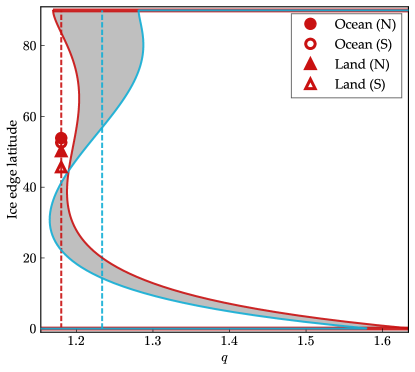
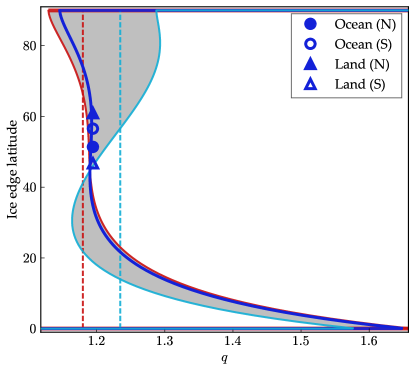
Figure 20: Ice edge latitude as a function of the parameter $q$ (see Section 2.1) from the analytical annual energy balance model (Rose et al., 2017), for the cases shown in Figures 17 (left) and 18 (right). The solution is a function of obliquity: light blue corresponds to the minimum obliquity in the simulation, red to the maximum obliquity, and the gray-shaded area is the range explored by the planet. Vertical dashed lines indicate the value of $q$, which is a function of eccentricity, at the corresponding times. In the left panel, markers show the ice edge latitude for northern and southern land and ocean at the time of maximum obliquity, at the coeval value of $q$, which depends on the eccentricity. Triangles and circles represent land and ocean, respectively, while closed and open markers represent northern and southern hemispheres, respectively. The right panel also shows these ice edge latitudes and the analytical solution at 500 years before the planet becomes fully glaciated (dark blue).

Figure 20 shows the ice edge latitude as a function of the parameter $q$, from the Rose et al. (2017) solution, for the two cases discussed above (see Section 2.2). The dimensionless parameter $q$ describes the combined effects of insolation and greenhouse warming.

The panels in Figure 20 show the equilibrium ice edge latitude at different obliquities—the light blue line at each case’s minimum obliquity, and the red line at its highest obliquity. The gray shaded area indicates the full range of solutions the simulation explores. When the slope of the line is positive or zero (as in the upper and lower branches), the ice edge is in a stable equilibrium (the annual solution is an equilibrium model). When the slope is negative or undefined, the ice edge is unstable and gives rise to the small ice cap instability (SICI) at the highest latitudes, and the large ice cap instability (LICI) at the mid to low latitudes. When the ice edge is at 90^∘, there is no ice cap; when it is at 0^∘, the planet is in a snowball state.

The left-hand panel corresponds to the case that does not experience the LICI (Figure 17). In this case, there is always a stable branch for the ice edge at all obliquities. The points shown in the plot are the actual ice edge locations from our full seasonal model, for both the land and ocean in each hemisphere, at the time of the highest obliquity. The vertical dashed lines indicate the average annual value of $q$ (which depends on the eccentricity) at each obliquity extreme. These points lag the analytic ice edge solution (which represents the climate in equilibrium) in time, and are dependent on the seasonality and the nature of the ice sheet model, and so do not fall directly on the analytical solution at most times. Nevertheless, the points stay very near to the analytical solution, and give a sense of why the instability is avoided. In this case, the instability never occurs because the ice edges (land and ocean in each hemisphere) remain on a stable branch of the analytical solution at mid-latitudes (or retreat to $0^{\circ}$).

In the right-hand panel, we see the same quantities plotted for the second case (Figure 18), which experiences the LICI. We can see that at the highest obliquity (red curve), there is no stable ice edge between 0^∘ and 90^∘. We have additionally plotted the analytical solution $\sim 500$ years before the planet has fully entered the snowball state. We can see that the ice edges in each hemisphere are precariously perched upon a branch of the solution where the slope is becoming undefined. At this point, the ice must either retreat entirely or expand to the equator. Because this occurs near a minimum in global insolation (the eccentricity is low), and the ice sheets have high thermal inertia, the snowball state is more easily reached. This demonstrates the susceptibility of planets with large orbital/obliquity variations to the snowball instability. Essentially, if planets proceed to a high obliquity and low eccentricity state with ice sheets extending to mid-latitudes, the ice edge becomes unstable and the entire planet quickly freezes.

For the climate parameters we use here, this instability occurs when the obliquity reaches $\sim 35^{\circ}$. These climate parameters ($a_{0},A,B$, and $D$) are chosen to reproduce Earth’s atmosphere, however, a planet with different atmospheric properties will respond differently to this obliquity oscillation. For some types of atmospheres, the instability will occur at a different obliquity, for others, the instability may not occur at all (for a detailed exploration of the climate parameters, see Rose et al., 2017).

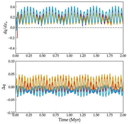
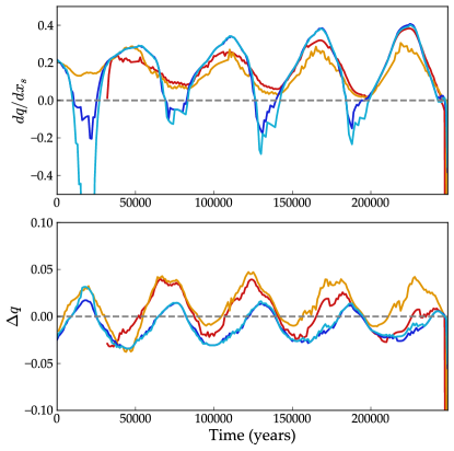
Figure 21: The quantities $dq/dx_{s}$ and $\Delta q$, which are related to the stability of ice caps in the annual EBM (see text), for a case with $P_{rot}=1.62$ day, $\varepsilon_{0}=23.5^{\circ}$, $e_{0}=0.167$, and $i_{0}=14.54^{\circ}$ (left) and $i_{0}=16.04^{\circ}$ (right). The quantities $dq/dx_{s}$ and $\Delta q$ are plotted as a function of time for the northern ice sheet on land (red), the southern ice sheet (orange), the northern sea ice (dark blue), and the southern sea ice (light blue). Negative values of $dq/dx_{s}$ indicate the ice cap is unstable in the annual model (but not necessarily in our seasonal model). Negative values of $\Delta q$ indicate that the average insolation is below that required to maintain the ice edge at its current latitude, suggesting that the ice should grow. In the left-hand case, the ice-cap is stable over the entire simulation. In the right-hand case, $dq/dx_{s}$ periodically dips below zero for the ocean in both hemispheres, but the snowball instability isn’t triggered until $dq/dx_{s}<0$ for land.

Figure 21 shows two parameters that can be used to analyze the ice edge stability: $dq/dx_{s}$ and $\Delta q$, for a clement (i.e. non-snowball) case with $P_{rot}=1.62$ day and $\varepsilon_{0}=23.5^{\circ}$. Both quantities are calculated at the ice edge latitude for northern and southern land and ocean, for a total of four ice edges. The “perturbation”, $\Delta q$, is

$$\Delta q=q_{true}-q_{equil},$$ (31)

where $q_{\text{true}}$ is the “true” value of $q$, calculated from the stellar flux and the eccentricity at that instant in time and $q_{\text{equil}}$ is calculated from the analytical solution, at each ice edge and the current obliquity. Thus, it is when both $dq/dx_{s}$ and $\Delta q$ are negative that we would expect the snowball states to occur—this corresponds to the third quadrant in the right panel of the figure. Both $dq/dx_{s}$ and $q_{\text{equil}}$ are calculated from the Python package developed in Rose et al. (2017), see Section 2.2.

As described previously, the ice caps will become unstable any time $dq/dx_{s}<0$. Whether or not the caps collapse to the poles or grow to the equator depends on the direction of the perturbation, $\Delta q$. Figure 21 (left panels) shows a case in which the ice edges are truly stable (except in the earliest phase, when the ice sheets are growing): $dq/dx_{s}>0$ over the entire simulation.

The same quantities are shown in Figure 21 (right panels) for an adjacent case which undergoes the snowball instability. In this case, $dq/dx_{s}$ becomes negative several times for the sea ice in both hemispheres and $\Delta q$ is negative during some of these excursions. The ice edges do not grow immediately to the poles, however. This may be due to the fact that the model is not in equilibrium, but since the sea ice is treated as a thin veneer that melts instantly when $T>-2$, the response time of the oceans to changes in insolation should be relatively short. Rose et al. (2017) shows that the seasonal model does deviate from the analytical solution; this is probably the reason the instability does not occur during those times.

Careful inspection of the upper right panel in Figure 21 shows that it is actually the northern ice sheet (red curve) that leads the way into the snowball state, not the sea ice in either hemisphere. It is interesting that this happens so quickly after $dq/dx_{s}$ becomes negative for this ice sheet, when the instability did not occur during previous excursions below zero. It is possibly a result of hysteresis: one may note that $\Delta q$ at the northern ice edge was fairly large and positive during the first three eccentricity cycles. During the fourth ($\sim 220,000$ years), however, $\Delta q$ barely exceeds zero before $dq/dx_{s}$ becomes negative. In other words, the ice sheet receives strong heating during all of the previous three eccentricity maxima, but very weak heating during the last, which leaves it poised, so to speak, to continue growing the next time $dq/dx_{s}<0$.

The analytical theory does not always provide a simple explanation, as it does for the case shown in Figure 21. Figure 22 shows another nearby case that undergoes the snowball instability. For most of the simulations, whenever $dq/dx_{s}<0$, $\Delta q$ is positive. At these times the sea ice usually disappears entirely (gaps in the blue curves left panels). The occurrence of a snowball state at $\sim 750$ kyr may be a result of hysteresis again—$\Delta q$ does undergo a negative period shortly prior to the snowball state, but this period does not appear significantly different from the cycles before it.

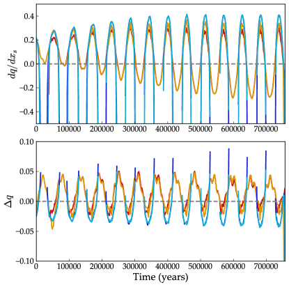
Figure 22: Same as Figure 21, but for $P_{rot}=1.62$ day, $\varepsilon_{0}=23.5^{\circ}$, $e_{0}=0.167$, and $i_{0}=18.96^{\circ}$. This case enters a snowball state at $\sim 750,000$ years. The northern and southern sea ice caps melt completely numerous times prior to the instability at $\sim 760$ kyr—shown as gaps in the blue curves. Eccentricity and obliquity are high during these times.

4.4 Relative importance of obliquity, eccentricity and COPP

With orbital and obliquity cycles as large as our test planet here, the periodicity of the ice is plainly visible. It is interesting, still, to perform periodogram analysis to understand the relative importance of the three insolation parameters: obliquity, eccentricity, and COPP. We calculate periodograms for each of these variables, for the ice sheet heights at $65^{\circ}$ north and south, and for the total global ice mass. These are calculated using the periodogram function in the SciPy package for Python, with a Bartlett window function to produce a clean power spectrum (Jones et al., 2001–2017).

We first perform a periodogram analysis on a static, but eccentric case. Under our “static” conditions, the orbit and obliquity do not change, but we can still allow the spin axis to precess according to Equation (12) in Paper I. This results in a sinusoidal variation in COPP. This parameter is typically the weakest of the three insolation parameters, so this example, which has no variation in $\varepsilon$ or $e$, allows us to see its effect more plainly. The ice sheets grow and decay in response to the planet’s precession. The total ice volume’s strongest peak is at half the period of COPP—this is because the northern and southern ice sheets grow and decay at opposing times.

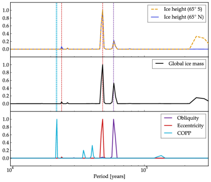
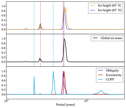
Figure 23: Normalized power spectra showing the strength at different periods in the ice height (top panel), global ice volume (middle panel), and the insolation parameters (obliquity, eccentricity, and COPP). Vertical dashed lines in the top two panels indicate peaks in the insolation parameters. The left panel shows a case with $P_{rot}=1.62$ day, $\varepsilon_{0}=23.5^{\circ}$, $e_{0}=0.167$, and $i_{0}=11.67^{\circ}$ and the right shows a case with $P_{rot}=1.62$ day, $\varepsilon_{0}=23.5^{\circ}$, $e_{0}=0.25$, and $i_{0}=16.04^{\circ}$. The ice sheets are strongly coupled to the eccentricity and, to lesser extent, the obliquity. The case on the right lies within the secular spin-orbit resonance, hence the obliquity and eccentricity have the same period of oscillation.

Figure 23 shows the periodograms for two cases with $P_{\text{rot}}=1.62$ day and $\varepsilon_{0}=23.5^{\circ}$ that are characteristic of the behavior we see over much of this parameter space. The left panel shows a case that is outside the secular resonance (see Figure 12) and the right shows a case that is inside the resonance. Outside the resonance, the obliquity and eccentricity have distinct peaks, and both can be seen in the ice sheet growth and decay. In the secular resonance, the obliquity oscillates with almost exactly the same period as the eccentricity (a consequence of resonance), and the ice sheets follow this period. Interestingly, in all of the parameter space we explore, the ice mass is dominated by the eccentricity cycle, not the obliquity cycle, except in the secular resonance, when the frequencies are similar and thus difficult to disentangle. The periods associated with COPP cannot even be seen in the ice sheets on a linear scale. The ice sheets are mostly driven by the eccentricity, while the obliquity controls their stability (Section 4.3).

4.5 Importance of ice sheets

The inclusion of the ice sheet model has important consequences. The snowball instability is triggered more easily (i.e., at higher $S_{\star}$), because of the extra energy required to melt the ice sheets (compared to the energy required simply to raise the surface temperature above freezing). Thus the climate with ice sheets is generally cooler at the same stellar flux than without. Indeed, without ice sheets, for our test planet at $\varepsilon=23.5^{\circ}$, the snowball state is not reached until $S/S_{0}\approx 0.95$, compared to $S/S_{0}\approx 0.975$ with ice sheets (Figure 7).

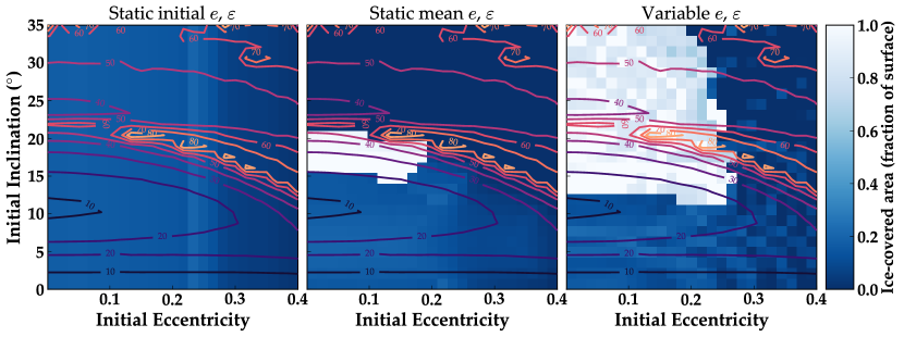
Figure 24: Fractional area of ice coverage at $\varepsilon_{0}=23.5^{\circ}$, $P_{rot}=1$ day, with ice sheets disabled. On the left are static conditions at the initial values; on the right, dynamic orbit and obliquity. Compare to Figure 10. The stellar flux here is lower than in the simulations from Figure 10, $S=1304$ W m^-2. The ice coverage is very different from the cases with ice sheets at low inclinations—in the lower left, where the obliquity variations are relatively small.

The response to orbital variations is altered as well. Figure 24 shows the fractional area coverage for $\varepsilon_{0}=23.5^{\circ}$, $P_{rot}=1$ day, at $S=1304$ W m^-2. Without perturbations, at this stellar flux, there are no snowball states. At $e\sim 0.25$, the area of ice coverage increases slightly, because of increased apoastron distances and time spent there, but the ice coverage drops to zero at the highest eccentricities. When perturbations are included, the area of ice coverage increases in most regions and snowball states are reached at $i_{0}\gtrsim 12^{\circ}$ and $e_{0}\lesssim 0.25$. The change in ice coverage between static and dynamic cases is more pronounced here than in the low obliquity cases with ice sheets (Figure 10). Further, the region of small obliquity variations (lower left) does not experience snowball states as often as the cases with ice sheets.

4.6 Comparison with Armstrong et al. (2014)

Here, we revisit the 17 test systems from Armstrong et al. (2014). Refer to that paper for the physical details of these systems. We simulate the orbital evolution using DISTORB and HNBody and the obliquity evolution using DISTROT. In cases 1, 2, 5, 6, 7, 13, 14, and 17, the combined orbital/obliquity evolution resulting from the secular model (DISTORB) matches sufficiently well with Armstrong et al. (2014), and we couple these directly to the climate model, POISE. In the rest of the cases, the eccentricity and/or obliquity evolution (using DISTORB) diverges significantly from the Armstrong et al. (2014) simulations or the semi-major axis evolution is large enough that we must use HNBody for the orbital evolution. Whether we ultimately use DISTORB or HNBody, we ensure that the obliquity/orbital evolution matches well with Armstrong et al. (2014) before running the climate model.

In all cases, we run the climate model with the same parameters and initial conditions as for our Earth comparison (Section 3) and the Earth-mass planet in our test system. For each system, we run three sets of POISE simulations: one set with the orbit and obliquity held constant at their initial values, one set with the orbit and obliquity held constant at their mean values (over 1 Myr), and one set with the full orbital and obliquity variations.

We generate a comparison with Armstrong et al. (2014) by varying the stellar luminosity and locating the value, $L_{\text{OHZ}}$, at which the transition between warm, clement conditions and the snowball state occurs. The semi-major axis at which the outer edge of the habitable zone (OHZ) occurs is then calculated from

$$a_{\text{OHZ}}=a_{\oplus}\sqrt{\frac{L_{\odot}}{L_{\text{OHZ}}}}.$$ (32)

The purpose of this somewhat awkward definition is solely to compare directly with Armstrong et al. (2014). We do not vary the initial semi-major axis of the planet ($a_{0}=1$ au in every case) because the eccentricity and obliquity evolution would be different at every location. Varying the stellar luminosity instead gives us a way of isolating the effects of the dynamical evolution. This definition of $a_{\text{OHZ}}$ is also not fully self-consistent because in several cases (systems 4, 10, and 11), the semi-major axis of the planet varies by $\sim 10\%$, leading to a significant change in the stellar flux received by the planet. This ultimately leads to a significant decrease ($\sim 6-8\%$) in $a_{\text{OHZ}}$ for these three cases. In reality, it is probably more accurate to describe this result as an excursion beyond the habitable zone due to an increase in semi-major axis $a$, rather than a decrease in the distance at which the planet enters a snowball state. Such is the difficulty in reducing a concept as multi-faceted as orbital evolution to a single parameter, $a_{\text{OHZ}}$.

The percent enhancement of the OHZ is then calculated for each system relative to system 1 and displayed in Figure 25 for the static initial, static mean, and variable orbit and obliquity (compare to Figure 11 in Armstrong et al. (2014)). Note also that system 1 has the same $a_{\text{OHZ}}$ for the static initial, static mean, and variable orbit/obliqiuty values, so the percent enhancement for each is zero. In most cases, the change in $a_{\text{OHZ}}$ from system 1 is $\lesssim 1\%$. The OHZ is enhanced under static initial conditions for systems 3, 10, and 15 as a result of the high initial eccentricity of the planet. In systems 2, 3, 5, 6, 15, and 16, the enhancement under static mean conditions is a result of the planet’s high mean obliquity. Variations enhance the OHZ relative to system 1 only in systems 3 and 15, which also saw warmer conditions due to the higher initial eccentricity. For the most part, the variations lead to a decrease in $a_{\text{OHZ}}$. Except in cases where there was no change to the OHZ, variations always lead to a decrease in the $a_{\text{OHZ}}$ compared to static conditions in the same system.

Ultimately, our results are significantly different from Armstrong et al. (2014). Compare our Figure 25 with their Figure 11. We find that, in general, dynamical evolution of the eccentricity and obliquity of a HZ planet tends to make the planet more susceptible to snowball states than when it has static orbital conditions, while Armstrong et al. (2014) found that dynamical variations tended to inhibit glaciation and snowball states. There are two fundamental reasons our results differ from that study.

The first is related to the parameterization of the OLR. The stability of the EBM is related to the strength of the longwave (LW) radiation feedback and the ice-albedo feedback. The LW radiation feedback is negative: a small positive perturbation to the surface temperature will cause the OLR to increase, generating more cooling and returning the surface to the unperturbed temperature. The process also works in the other direction: a small negative perturbation to the temperature will cause the OLR to decrease, creating additional heating and returning the temperature to its previous value. The ice-albedo feedback is positive: a small negative perturbation to the surface temperature will cause the ice to grow, reflecting more radiation to space and causing the surface to cool further. A positive perturbation will likewise generate runaway warming, if the ice-albedo feedback is the dominant feedback of the model. Of course, the real Earth and more sophisticated 3D models have a number of other feedback processes that work to alter the climate stability, but in a 1D EBM like ours and the model in Armstrong et al. (2014), stability is simply a LW competition between the radiation feedback and the ice-albedo feedback.

In this simple formulation, the LW radiation feedback is contained within the parameter $B$. A large, positive value of $B$ will create a very stable climate, while a smaller value will create a less stable climate. For Earth, $B\approx 2.09$ W m^-2 K^-1 (North & Coakley, 1979). A Taylor expansion of the OLR parameterization in Spiegel et al. (2009), for example, shows that their model 2 has $B\approx 2.28$ W m^-2 K^-1 at a surface temperature of 288 K, and so their model should be more stable against snowball states when using this formulation than with the OLR from North & Coakley (1979).

The OLR from Armstrong et al. (2014) is found by combining their Equations (23) and (24) and comparing to the full energy balance equation (our Equation 2):

$$I(T)=\frac{\epsilon_{s}\sigma T_{s}^{4}}{1+\tau}-F_{\text{surf}},$$ (33)

where $\epsilon_{s}$ is the emissivity of the atmosphere, $\sigma$ is the Stefan-Boltzmann constant, $F_{\text{surf}}$ is a tunable constant and $\tau$ is a tunable parameter used to approximate the greenhouse effect that was not assumed to be a function of temperature. The authors found that setting $\epsilon_{s}=1$ and $\tau=0.095$ reproduced Earth and so fixed these values for the rest of the study. As stated before, a Taylor expansion of Equation 33 with respect to temperature gives the value of $B$:

$$B=\frac{dI}{dT}=\frac{4\epsilon_{s}\sigma T_{s}^{3}}{1+\tau}.$$ (34)

Plugging in their constants and a surface temperature of $T_{s}=288$ K, one finds $B=4.95$ W m^-2 K^-1. As far as EBMs go, this model is extremely stable against the snowball instability.

The second reason our model differs from Armstrong et al. (2014) is our inclusion of the horizontal heat transport (however crudely it is represented here). A comparison between our energy balance equation (2) and that in Armstrong et al. (2014) shows that $D=0$ in the latter. It can be shown that when $D=0$, the ice-albedo feedback does not affect adjacent latitudes as it should. Conceptually, ice-albedo feedback occurs because, for example, when the albedo (and thus temperature) changes in one model cell, the temperature gradient between adjacent cells is changed. This causes the heat flow between cells to change. The feedback works because cooling (or heating) in one cell alters heat flow to and from adjacent cells, cooling (or heating) those adjacent areas. Without that horizontal heat flow, there is no ice-albedo feedback, and no snowball instability—that is, snowball states can still occur, but only when all latitudes in the model individually come into radiative equilibrium at below freezing temperatures. That occurs at a much lower stellar flux than that caused by the instability.

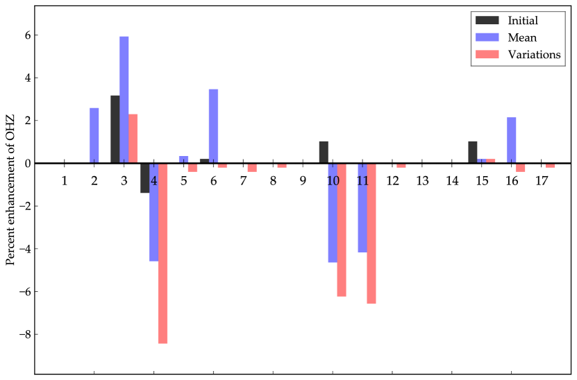
Figure 25: Percent enhancement in the distance to the OHZ from the host star for the 17 systems in Armstrong et al. (2014). The percent enhancement for each system is measured relative to system 1, like in Armstrong et al. (2014). Black bars are for static orbits and obliquity at the initial values, blue bars are for static orbits and obliquity at the mean values, and red bars are for variable orbits and obliquity. In cases 4, 10, and 11, the semi-major axis of the Earth-mass planet varies by $\sim 10\%$, leading to large changes in insolation and subsequent snowball states. In cases 2, 3, 5, 6, 15, and 16, the large mean obliquity leads to an extension of the habitable zone for static mean conditions. In most systems, variable eccentricity and obliquity leads decrease in the OHZ distance.

4.7 Predicting climate states with machine learning

Results from the statistical analysis and machine learning model are shown in Tables 5 and 6. Correlations are strongest with stellar flux, $S$, and the eccentricity parameters. The MIC values are similar $\sim 0.2-0.3$ across most of the parameters, except for $\varepsilon$’s relationship to $\delta_{\text{snow}}$. Interestingly, $\Delta i$ shows a stronger correlation, $R$, with $\delta_{\text{snow}}$ and $f_{\text{ice}}$ than the obliquity parameters, despite the fact that the inclination has no direct impact on climate. The linear relationships ($R$) between ($f_{\text{ice}}$, $i_{0}$), ($f_{\text{ice}}$, $\langle i\rangle$), ($\delta_{\text{snow}}$, $i_{0}$), and ($\delta_{\text{snow}}$, $\varepsilon_{0}$) are insignificant if a $p-$value of $<0.005$ is desired (see Section 2.3). However, the MIC for these quantities shows a non-linear relationship about as strong as any other parameter. One plausible explanation is that the inclination (especially the variation in inclination) affects both the evolution of the eccentricity and the evolution of the obliquity (see Equations 5,6, 12, and 13 in Paper I), and thus is indirectly coupled to the climate through two variables.

The stellar flux, $S_{\star}$ (defined here for a circular orbit), is unsurprisingly the most important parameter in determining the final climate parameters, $\delta_{\text{snow}}$ and $f_{\text{ice}}$. The mean eccentricity, $\langle e\rangle$, tends to be the next most important parameter, as expected (see Equation 1). The remaining variables tend to have similar, and relatively small, weighting. About half the time, one could correctly predict the climate state of our test planet with the stellar flux and the mean insolation. However, including all variables, the ML model can predict $\delta_{\text{snow}}$ correctly 97% of the time, and $f_{\text{ice}}$. For the RF regressor, the accuracy metric is the $R^{2}$ score, which in this case is $R^{2}=0.93$ (the best possible score is 1). The similar weights of the remaining variables illustrates the complexity of the interplay between orbit and climate. Note that feature importances should be interpreted cautiously as correlations between features can skew the features—for example, in the case of two highly-correlated features, one feature can display a high importance ($\xi_{i}$), while the second displays a low importance.

Table 5: Relative importance of input parameters on $\delta_{\text{snow}}$

Parameter	Pearson $R$ ($p$)	MIC	$\zeta_{NL}$	$\xi_{i}$
$S_{\star}$	-0.517486 (0.0)	0.259659	-0.008133	0.367391
$e_{0}$	-0.469633 (0.0)	0.191850	-0.028705	0.088580
$\Delta e$	-0.281968 (0.0)	0.181865	0.102360	0.014340
$\langle e\rangle$	-0.480688 (0.0)	0.256887	0.025826	0.227943
$i_{0}$	0.026494 (0.0132)	0.256149	0.255448	0.022177
$\Delta i$	-0.318399 (0.0)	0.216146	0.114768	0.024869
$\langle i\rangle$	0.056757 ($1.08\times 10^{-7}$)	0.200756	0.197534	0.047204
$\varepsilon_{0}$	-0.026059 (0.01478)	0.000490	-0.000189	0.015797
$\Delta\varepsilon$	0.084789 ($1.95\times 10^{-15}$)	0.097013	0.089824	0.094639
$\langle\varepsilon\rangle$	-0.031998 (0.00276)	0.124936	0.123913	0.097059

Table 6: Relative importance of input parameters on $f_{\text{ice}}$

Parameter	Pearson $R$ ($p$	MIC	$\zeta_{NL}$	$\xi_{i}$
$S_{\star}$	-0.502261 (0.0)	0.260615	0.008349	0.396097
$e_{0}$	-0.498351 (0.0)	0.268657	0.020303	0.085960
$\Delta e$	-0.322404 (0.0)	0.218874	0.114929	0.012151
$\langle e\rangle$	-0.515085 (0.0)	0.295807	0.030495	0.249936
$i_{0}$	-0.011158 (0.2967)	0.255632	0.255508	0.016456
$\Delta i$	-0.361029 (0.0)	0.216911	0.086569	0.021697
$\langle i\rangle$	0.020870 (0.0509)	0.199982	0.199546	0.036169
$\varepsilon_{0}$	-0.062202 ($5.77\times 10^{-9}$)	0.170839	0.166970	0.018088
$\Delta\varepsilon$	0.059806 ($2.16\times 10^{-8}$)	0.148690	0.145113	0.079007
$\langle\varepsilon\rangle$	-0.092422 ($4.61\times 10^{-18}$)	0.242192	0.233650	0.084440

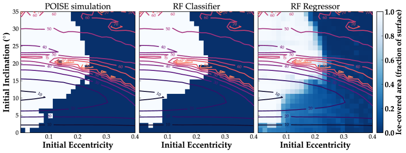
Figure 26: Snowball states ($\delta_{\text{snow}}$) for $P_{rot}=1$ day and initial obliquity $\varepsilon_{0}=23.5^{\circ}$, with a stellar constant of $S=1332.27$ W m^-2 from the full orbit/climate simulation (left) and the machine learning algorithm (RF classifier; middle). White regions are simulations that ended in a snowball state; dark blue are those that did not. In the ML case shown here, this slice ($P_{rot}=1$ and $\varepsilon_{0}=23.5^{\circ}$) of parameter space was excluded from the training set and the algorithm was trained on the remaining data. The right panel shows the fractional ice coverage area for $P_{rot}=1$ day and initial obliquity $\varepsilon_{0}=23.5^{\circ}$, with a stellar constant of $S=1332.27$ W m^-2, as predicted by the random forest regressor. Compare to the right panel in Figure 10.

Figure 26 shows $\delta_{\text{snow}}$ for the full orbit$+$climate simulations (left), compared to the ML algorithm predictions (middle), for one slice of our parameter space. The ML algorithm captures the basic shape of the parameter space, though it does miss a few features such as the blue island at $e\approx 0.15$ and $i_{0}\approx 20^{\circ}$. In the case shown, this slice of parameter space ($P_{rot}=1$ day, $\varepsilon_{0}=23.5^{\circ}$, and $S=1332.27$ W m^-2) was excluded from the training set. In the right panel, we show the predicted ice area coverage for $P_{rot}=1$ day and initial obliquity $\varepsilon_{0}=23.5^{\circ}$ at $S=1332.27$ W m^-2. Again, this slice was excluded from the training set. Though the model does slightly better at predicting $\delta_{\text{snow}}$, the algorithm picks out the structure of the original map of $f_{\text{ice}}$ (Figure 10).

We conclude that the ML algorithm does very well at predicting the ultimate climate state of this test planet. Though we trained the model on a fixed grid of initial conditions, future studies will probe training sets created with randomized initial conditions. Future analyses will be able to extend the model beyond what is computational feasible via direct integration: when it becomes prohibitive to run a desired number of simulations, we may be able to make do with a fraction of that number when we apply ML.

5 Discussion

We reiterate our primary conclusions here:

1. In predicting the climate state of a potentially habitable planet, it is not enough to simply run a climate model with the initial conditions (i.e. the observed orbit), nor is it sufficient to use the averaged quantities. Variations in the orbit need to be considered, because of the instability brought on by coupled obliquity and eccentricity variations. In particular, we note the instability that occurs when the planet’s obliquity reaches $\sim 35^{\circ}$ during an eccentricity minimum, if a large ice cap is present. At this obliquity, with the climate parameters we use here, there is no stable location for the ice edge; it must either retreat or grow uncontrollably. If the incoming stellar flux is decreased because the eccentricity is low, the ice will grow to the equator. If the eccentricity is sufficiently high at such times, the ice caps will collapse entirely.

2. Coupled orbital and obliquity variations tend to trigger the snowball instability. The eccentricity oscillations cause the global flux to vary and as a result, the planet can go from completely ice free to having large ice caps in a few thousand years. If the obliquity remains low enough, the ice caps remain stable. When the obliquity is oscillating by a large amount, however, the ice latitude can become suddenly unstable. Many times, the ice caps are small enough that they disappear entirely (the small ice cap instability); other times, the ice caps are large enough to trigger the large ice cap instability and the planet becomes entirely ice covered.

3. For eccentricity variations this large ($\Delta e\sim 0.1-0.3$), the ice ages are primarily controlled by the eccentricity, not the obliquity. This is very different from the recent Earth, where the insolation variations are dominated by the obliquity cycle. Obliquity is important mainly in determining the stability and location of ice sheets.

4. The thermal inertia of ice sheets plays an important role. The inclusion of ice sheets causes snowball states to be triggered at higher incident stellar flux than if a simple temperature dependent albedo is used to mimic ice. Interestingly, the difference between static and dynamic orbital conditions seems to be reduced somewhat by the presence of ice sheets. The model is more susceptible to snowball states in general, but ice sheets somewhat diminish the response of the climate to orbital variations.

In summary, planets undergoing strong orbital forcing are prone to the snowball or large ice cap instability, and surface habitability is therefore compromised. It should be noted, however, that Earth potentially went through several snowball states during the Proterozoic Eon ($\sim 2.5$ to $0.54$ billion years ago), and photosynthetic life persisted during these phases (Harland, 1964; Kirschvink, 1992). One explanation is that the surface was not actually completely frozen during such time periods—the Earth was in a “soft” snowball (or “water-belt”) state, with some open ocean in the tropics (Chandler & Sohl, 2000). An alternative explanation is that meltwater ponds persisted on the surface of the ice, creating a refuge for photosynthetic life (Hoffman et al., 2017). Unfortunately, the EBM does not capture all the necessary physics to distinguish a soft snowball state from a hard snowball state. Therefore, our results are probably pessimistic in regard to surface habitability.

Modeling of Exo-Milankovitch cycles is difficult because of the timescales involved. 3D GCMs can take weeks to converge for static orbital conditions and decade long integrations. We have approached the problem with a comparatively simple, computationally efficient EBM—however, such models lack important phenomena and thus must be treated cautiously. As much as possible, we attempt to validate our results against a more sophisticated model. In terms of average yearly behavior, the EBM does a decent job. The greatest discrepancies occur in simulations that reach high obliquity and have relatively high stellar flux. In these cases, the summer insolation at the poles can be intense enough (locally) to reach runaway greenhouse temperatures. Undoubtedly, there will also be cloud formation, which affects the albedo, as observed in GCM simulations of synchronous rotators (Joshi, 2003; Edson et al., 2011, 2012; Yang et al., 2013). The difference is that here, the planet is in a very different rotation state, which may inhibit the global scale redistribution of heat seen in those studies.

The carbon-silicate cycle on a planet like Earth is probably too slow to prevent orbitally induced snowball states. Earth’s carbon-silicate cycle operates on a $\sim 0.5$ Myr time-scale (Kasting et al., 1993; Haqq-Misra et al., 2016); the planet in this configuration can evolve from ice-free to completely ice-covered in thousands of years. If a planet has significantly higher outgassing rate and weathering rates than Earth, there may be some hope of preventing the instability through this negative feedback. Even with an Earth-like carbon-silicate cycle, however, the snowball states could eventually be escaped by building atmospheric carbon dioxide pressure. The planet may then become extremely warm for an extended period until carbon is weathered out of the atmosphere. And, of course, the obliquity and eccentricity will continue to vary in the same manner as before, perhaps leading to periods of intense polar heating. A long term simulation of exo-Milankovitch cycles with a carbon cycle would certainly be interesting.

In Paper I, we discussed possibilities for determining whether an exoplanet is undergoing Milankovitch cycles. As mentioned there, constraining this phenomenon will largely rely on two-dimensional mapping techniques (Pallé et al., 2008; Cowan et al., 2009; Kawahara & Fujii, 2010; Fujii & Kawahara, 2012; Cowan et al., 2013; Kawahara, 2016; Schwartz et al., 2016). A 2-D map of the surface and/or atmosphere of an exoplanet will be difficult to generate and will most likely require a large telescope such as the Large UltraViolet Optical and InfraRed surveyor (LUVOIR; Bolcar et al., 2015; Dalcanton et al., 2015).

Planets such as we have investigated here, with large amplitude obliquity and eccentricity cycles, would be ideal cases for constraining Milankovitch cycles. Referring to Figures 10 - 15, and comparing the left and right panels in each, we can see that there are regions of parameter space where we expect the planet to be in a snowball state under static obliquity/orbital conditions, but it is clement when these parameters are allowed to vary. We also see many regions where the planet is warm under static conditions, but enters a snowball state when variations are included. By comparing the climate state under static and dynamic scenarios with observed 2-D albedo maps, it might be possible to infer that the planet is undergoing Milankovitch cycles. This will, of course, depend heavily on one’s trust in the climate models used and the elimination of alternative explanations.

For the nearer future, the more practical application of the type of modeling we present here is target prioritization. In scenarios where the orbital parameters of a potentially habitable planet and its companions are well constrained, modeling of dynamical effects on climate (such as Milankovitch cycles) may better inform the likelihood of surface habitability. If there appears to be a high probability of snowball states due to such variations, the target will be less favorable than another for detecting surface biosignatures. Conversely, if one is primarily interested in determining the presence of Milankovitch cycles, a target in a dynamically “hot” system will be preferable. Regardless of motivation, our understanding of the coupling of climate to obliquity and orbital variations will be important to the interpretation of LUVOIR observations.

6 Conclusions

In Paper I, we showed that secular spin-orbit resonances can exist even in relatively simple planetary systems, and that they can cause very large obliquity oscillations. In this paper, we applied a climate model to one of these systems. We have modeled the climate evolution of a planet with an Earth-like atmosphere in response to extreme orbital forcing. The large changes in eccentricity and obliquity drive the growth and retreat of ice caps, which can extend from the poles to $\sim 30^{\circ}$ latitude. These exo-Milankovitch cycles often lead to the snowball instability, in which the planet’s oceans become completely ice covered, as well as the small ice cap instability, in which the ice completely disappears.

We reiterate that planetary systems are extremely complex, and in cases like that shown here, the presence of companions can affect an Earth-like planet’s habitability. It is particularly important to understand the eccentricity and obliquity evolution in combination, because the stability of ice sheets is intimately coupled to the obliquity and the eccentricity affects the amount of intercepted stellar energy. At a single stellar flux, a planet can be either clement and habitable or completely ice-covered, depending on the orbital parameters and the planet’s recent climate history. This further complicates the concept of a static habitable zone based on the stellar flux. We have shown that orbital and obliquity evolution, and the long time scales of ice evolution, should be considered when assessing a planet’s potential habitability.

7 Acknowledgements

This work was supported by the NASA Astrobiology Institute’s Virtual Planetary Laboratory under Cooperative Agreement number NNA13AA93A. This work was facilitated though the use of advanced computational, storage, and networking infrastructure provided by the Hyak supercomputer system at the University of Washington. The results reported herein benefited from the authors’ affiliation with the NASA’s Nexus for Exoplanet System Science (NExSS) research coordination network sponsored by NASA’s Science Mission Directorate. Thank you to David Crisp, Andrew Lincowski, Tony Del Genio, Ravi Kopparapu, Jacob Haqq-Misra, and Natasha Batalha for helpful discussions, and to the anonymous referee, whose feedback resulted in a greatly improved manuscript.

References

- Abe-Ouchi et al. (2013) Abe-Ouchi, A., Saito, F., Kawamura, K., et al. 2013, Nature, 500, 190
- Albanese et al. (2013) Albanese, D., Filosi, M., Visintainer, R., et al. 2013, Bioinformatics, 29, 407. +http://dx.doi.org/10.1093/bioinformatics/bts707
- Armstrong et al. (2014) Armstrong, J. C., Barnes, R., Domagal-Goldman, S., et al. 2014, Astrobiology, 14, 277
- Barkstrom et al. (1990) Barkstrom, B. R., Harrison, E. F., & Lee, III, R. B. 1990, EOS Transactions, 71, 279
- Berger (1978) Berger, A. L. 1978, Journal of Atmospheric Sciences, 35, 2362
- Bolcar et al. (2015) Bolcar, M. R., Balasubramanian, K., Clampin, M., et al. 2015, in Proc. SPIE, Vol. 9602, Optics for EUV, X-Ray, and Gamma-Ray Astronomy VII, 960209
- Bolmont et al. (2016) Bolmont, E., Libert, A.-S., Leconte, J., & Selsis, F. 2016, A&A, 591, A106
- Braithwaite & Zhang (2000) Braithwaite, R. J., & Zhang, Y. 2000, Journal of Glaciology, 46, 7
- Brasser et al. (2014) Brasser, R., Ida, S., & Kokubo, E. 2014, MNRAS, 440, 3685
- Breiman (2001) Breiman, L. 2001, Machine Learning, 45, 5. https://doi.org/10.1023/A:1010933404324
- Budyko (1969) Budyko, M. I. 1969, Tellus, 21, 611
- Cahalan & North (1979) Cahalan, R. F., & North, G. R. 1979, Journal of Atmospheric Sciences, 36, 1178
- Chandler & Sohl (2000) Chandler, M. A., & Sohl, L. E. 2000, J. Geophys. Res., 105, 20737
- Charnay et al. (2013) Charnay, B., Forget, F., Wordsworth, R., et al. 2013, Journal of Geophysical Research (Atmospheres), 118, 10
- Clark & Pollard (1998) Clark, P. U., & Pollard, D. 1998, Paleoceanography, 13, 1
- Cowan et al. (2013) Cowan, N. B., Fuentes, P. A., & Haggard, H. M. 2013, MNRAS, 434, 2465
- Cowan et al. (2009) Cowan, N. B., Agol, E., Meadows, V. S., et al. 2009, ApJ, 700, 915
- Crank et al. (1947) Crank, J., Nicolson, P., & Hartree, D. R. 1947, Proceedings of the Cambridge Philosophical Society, 43, 50
- Dalcanton et al. (2015) Dalcanton, J., Seager, S., Aigrain, S., et al. 2015, ArXiv e-prints, arXiv:1507.04779
- Deitrick et al. (2017) Deitrick, R., Barnes, R., Quinn, T. R., et al. 2017, ArXiv e-prints, arXiv:1712.10060
- Dressing et al. (2010) Dressing, C. D., Spiegel, D. S., Scharf, C. A., Menou, K., & Raymond, S. N. 2010, ApJ, 721, 1295
- Dunn (1959) Dunn, O. J. 1959, Ann. Math. Statist., 30, 192. https://doi.org/10.1214/aoms/1177706374
- Edson et al. (2011) Edson, A., Lee, S., Bannon, P., Kasting, J. F., & Pollard, D. 2011, Icarus, 212, 1
- Edson et al. (2012) Edson, A. R., Kasting, J. F., Pollard, D., Lee, S., & Bannon, P. R. 2012, Astrobiology, 12, 562
- Ferreira et al. (2014) Ferreira, D., Marshall, J., O’Gorman, P. A., & Seager, S. 2014, Icarus, 243, 236
- Forgan (2016) Forgan, D. 2016, MNRAS, 463, 2768
- Fretwell et al. (2013) Fretwell, P., Pritchard, H. D., Vaughan, D. G., et al. 2013, The Cryosphere, 7, 375
- Fujii & Kawahara (2012) Fujii, Y., & Kawahara, H. 2012, ApJ, 755, 101
- Glen (1958) Glen, J. W. 1958, Nature, 182, 1560
- Haqq-Misra et al. (2016) Haqq-Misra, J., Kopparapu, R. K., Batalha, N. E., Harman, C. E., & Kasting, J. F. 2016, ApJ, 827, 120
- Harland (1964) Harland, W. B. 1964, Geologische Rundschau, 54, 45
- Hays et al. (1976) Hays, J. D., Imbrie, J., & Shackleton, N. J. 1976, Science, 194, 1121
- Hoffman et al. (2017) Hoffman, P. F., Abbot, D. S., Ashkenazy, Y., et al. 2017, Science Advances, 3, e1600983
- Huybers & Tziperman (2008) Huybers, P., & Tziperman, E. 2008, Paleoceanography, 23, PA1208
- Imbrie & Imbrie (1980) Imbrie, J., & Imbrie, J. Z. 1980, Science, 207, 943
- Jenson et al. (1996) Jenson, J. W., Macayeal, D. R., Clark, P. U., Ho, C. L., & Vela, J. C. 1996, J. Geophys. Res., 101, 8717
- Jones et al. (2001–2017) Jones, E., Oliphant, T., Peterson, P., et al. 2001–2017, SciPy: Open source scientific tools for Python, , , [Online; accessed August 2017]. http://www.scipy.org/
- Joshi (2003) Joshi, M. 2003, Astrobiology, 3, 415
- Kasting et al. (1993) Kasting, J. F., Whitmire, D. P., & Reynolds, R. T. 1993, Icarus, 101, 108
- Kawahara (2016) Kawahara, H. 2016, ApJ, 822, 112
- Kawahara & Fujii (2010) Kawahara, H., & Fujii, Y. 2010, ApJ, 720, 1333
- Kirschvink (1992) Kirschvink, J. L. 1992, in The Proterozoic biosphere; a multidisciplinary study (Cambridge: Cambridge Univ. Press), 51–52
- Kopparapu et al. (2013) Kopparapu, R. K., Ramirez, R., Kasting, J. F., et al. 2013, ApJ, 765, 131
- Laskar et al. (1993) Laskar, J., Joutel, F., & Boudin, F. 1993, A&A, 270, 522
- Leconte et al. (2013a) Leconte, J., Forget, F., Charnay, B., Wordsworth, R., & Pottier, A. 2013a, Nature, 504, 268
- Leconte et al. (2013b) Leconte, J., Forget, F., Charnay, B., et al. 2013b, A&A, 554, A69
- Lefebre et al. (2002) Lefebre, F., Gallée, H., van Ypersele, J.-P., & Huybrechts, P. 2002, Annals of Glaciology, 35, 391
- Lisiecki (2010) Lisiecki, L. E. 2010, Nature Geoscience, 3, 349
- Lisiecki & Raymo (2007) Lisiecki, L. E., & Raymo, M. E. 2007, Quaternary Science Reviews, 26, 56
- Lissauer et al. (2012) Lissauer, J. J., Barnes, J. W., & Chambers, J. E. 2012, Icarus, 217, 77
- Maslin (2016) Maslin, M. 2016, Nature, 540, 208
- Miguel & Brunini (2010) Miguel, Y., & Brunini, A. 2010, MNRAS, 406, 1935
- North & Coakley (1979) North, G. R., & Coakley, Jr., J. A. 1979, Journal of Atmospheric Sciences, 36, 1189
- Pallé et al. (2008) Pallé, E., Ford, E. B., Seager, S., Montañés-Rodríguez, P., & Vazquez, M. 2008, ApJ, 676, 1319
- Paterson (1994) Paterson, W. S. B. 1994, The physics of glaciers, Oxford, OX, England ; Tarrytown, N.Y., U.S.A.: Pergamon
- Pedregosa et al. (2011) Pedregosa, F., Varoquaux, G., Gramfort, A., et al. 2011, Journal of Machine Learning Research, 12, 2825
- Press et al. (1987) Press, W. H., Flannery, B. P., Teukolsky, S. A., Vetterling, W. T., & Gould, H. 1987, American Journal of Physics, 55, 90
- Rauch & Hamilton (2002) Rauch, K. P., & Hamilton, D. P. 2002, in Bulletin of the American Astronomical Society, Vol. 34, AAS/Division of Dynamical Astronomy Meeting #33, 938
- Raymo (1997) Raymo, M. E. 1997, Paleoceanography, 12, 577
- Reshef et al. (2011) Reshef, D. N., Reshef, Y. A., Finucane, H. K., et al. 2011, Science, 334, 1518. http://science.sciencemag.org/content/334/6062/1518
- Roe (2006) Roe, G. 2006, Geophys. Res. Lett., 33, L24703
- Rose et al. (2017) Rose, B. E. J., Cronin, T. W., & Bitz, C. M. 2017, ApJ, 846, 28
- Schwartz et al. (2016) Schwartz, J. C., Sekowski, C., Haggard, H. M., Pallé, E., & Cowan, N. B. 2016, MNRAS, 457, 926
- Sellers (1969) Sellers, W. D. 1969, Journal of Applied Meteorology, 8, 392
- Selsis et al. (2007) Selsis, F., Kasting, J. F., Levrard, B., et al. 2007, A&A, 476, 1373
- Spiegel et al. (2008) Spiegel, D. S., Menou, K., & Scharf, C. A. 2008, ApJ, 681, 1609
- Spiegel et al. (2009) —. 2009, ApJ, 691, 596
- Spiegel et al. (2010) Spiegel, D. S., Raymond, S. N., Dressing, C. D., Scharf, C. A., & Mitchell, J. L. 2010, ApJ, 721, 1308
- Tamayo et al. (2016) Tamayo, D., Silburt, A., Valencia, D., et al. 2016, ApJ, 832, L22
- van Woerkom (1953) van Woerkom, A. J. J. 1953, The Astronomical Theory of Climate Changes, ed. H. Shapley, 147
- Way & Georgakarakos (2017) Way, M. J., & Georgakarakos, N. 2017, ApJ, 835, L1
- Williams & Kasting (1997) Williams, D. M., & Kasting, J. F. 1997, Icarus, 129, 254
- Williams & Pollard (2002) Williams, D. M., & Pollard, D. 2002, International Journal of Astrobiology, 1, 61
- Williams & Pollard (2003) —. 2003, International Journal of Astrobiology, 2, 1
- Williams (1975) Williams, G. E. 1975, Geological Magazine, 112, 441
- Williams (1993) —. 1993, Earth Science Reviews, 34, 1
- Wordsworth et al. (2011) Wordsworth, R. D., Forget, F., Selsis, F., et al. 2011, ApJ, 733, L48
- Wunsch (2004) Wunsch, C. 2004, Quaternary Science Reviews, 23, 1001
- Yang et al. (2013) Yang, J., Cowan, N. B., & Abbot, D. S. 2013, ApJ, 771, L45