Towards a Quantitative Comparison of Magnetic Field Extrapolations and Observed Coronal Loops

Abstract

It is widely believed that loops observed in the solar atmosphere trace out magnetic field lines. However, the degree to which magnetic field extrapolations yield field lines that actually do follow loops has yet to be studied systematically. In this paper we apply three different extrapolation techniques — a simple potential model, a NLFF model based on photospheric vector data, and a NLFF model based on forward fitting magnetic sources with vertical currents — to 15 active regions that span a wide range of magnetic conditions. We use a distance metric to assess how well each of these models is able to match field lines to the 12,202 loops traced in coronal images. These distances are typically 1–2″. We also compute the misalignment angle between each traced loop and the local magnetic field vector, and find values of 5–12^∘. We find that the NLFF models generally outperform the potential extrapolation on these metrics, although the differences between the different extrapolations are relatively small. The methodology that we employ for this study suggests a number of ways that both the extrapolations and loop identification can be improved.

Accepted for Publication in ApJ: April 30, 2018

1 Introduction

It is universally accepted that magnetic fields play a critical role in a wide range of solar phenomena, such as the heating of the solar upper atmosphere, the origin of the solar wind, and the initiation of coronal mass ejections. Unfortunately, at present, accurate magnetic field measurements over a wide field of view are routinely available only in the solar photosphere, where the magnetic field is still dominated by the plasma pressure and the field is not force-free (e.g., Metcalf et al., 1995). This greatly complicates the use of photospheric measurements as a boundary condition for methods that use the force-free assumption to extrapolate the magnetic field into the solar chromosphere and corona.

One approach to addressing the mismatch between the photospheric measurements and the force-free condition is to preprocess the vector magnetic field observations so that they approximate what would be measured in the chromosphere, where the field does become force-free. The non-linear force-free (NLFF) code introduced by Wiegelmann et al. (2006) represents perhaps the most widely known example of this approach. Other codes implementing this idea include those presented by Valori et al. (2012), and Jiang & Feng (2013). These codes build on the earlier NLFF models of Wiegelmann (2004), Amari et al. (2006), and Wheatland (2007).

Recently, an alternative approach to modeling non-potential fields in the corona has been developed that does not rely on vector magnetic field measurements. Instead, the line-of-sight photospheric magnetic field is modeled as a superposition of magnetic sources. The currents associated with each of these sources is varied in order to optimize the agreement between loops traced in coronal images and the topology of the field (see, Aschwanden 2013a; Aschwanden & Malanushenko 2013; Aschwanden 2016; also see Malanushenko et al. 2012 for a variation on this approach).

Models of the magnetic field play a critical role in our ability to study coronal heating. For example, a number of studies have used magnetic field extrapolations to determine the relationship between heating rates and the properties of the field by comparing full active region hydrodynamic simulations to observations (e.g., Schrijver et al., 2004; Warren & Winebarger, 2007; Lundquist et al., 2008; Winebarger et al., 2008; Bradshaw & Viall, 2016; Ugarte-Urra et al., 2017). These studies have often found that a volumetric heating rate that scales approximately as $\bar{B}/L$, where $\bar{B}$ is the mean field strength and $L$ is the loop length, provides a good match between the simulation and the global properties of the observed active region.

Interestingly, the alternative approach, where measurements of intensity variations on individual loops or plasma parameters on individual loops are related to the properties of the associated field lines appears to have received relatively little attention (see Xie et al. 2017 for one such example). This is surprising given that the trend in solar instrumentation is towards higher spatial and temporal resolution. The High-Resolution Coronal Imager (Hi-C; Kobayashi et al. 2014) and the Interface Region Imaging Spectrograph (IRIS; De Pontieu et al. 2014), for example, achieve a spatial resolution of better than 360 km and cadences below 10 s.

One impediment to studying the relationship between the properties of individual loops and the properties of magnetic field lines is the difficultly of matching the two together. Since loops are projected onto a two dimensional plane, their three dimensional geometry is ambiguous, except in the rare case of stereoscopic observations. Perhaps more fundamentally, it is not clear how closely current extrapolation techniques reproduce the topological properties of the corona, and how force-free the corona is at each loop location. Coronal images certainly show many clear examples of loops, or at least partial segments of loops, but systematic comparisons between the different extrapolation techniques and these loops have yet to be carried out. Systematic studies of different NLFF extrapolation methods have generally focused on the more global properties of the field, such as the free energy or the helicity (see, for example, De Rosa et al. 2009 and DeRosa et al. 2015). Some previous studies have compared extrapolated field lines to loops reconstructed from stereoscopic observations, De Rosa et al. (2009) and Chifu et al. (2017), but these comparisons have been limited to only a few loops.

In this paper we perform systematic comparisons of several extrapolation techniques with loops traced in coronal images. We consider the Vertical-Current Approximation (VCA) NLFF method described in Aschwanden (2016) and the NLFF extrapolation method based on vector observations described in Wiegelmann et al. (2012). For reference, we also consider a simple potential field extrapolation. Observations of the photospheric field are taken from the Helioseismic and Magnetic Imager (HMI, Scherrer et al. 2012) on the Solar Dynamics Observatory (SDO). We apply all three methods to the 15 active regions analyzed in Warren et al. (2012), which represent a broad spectrum of active regions sizes and total magnetic fluxes. For each of these regions we trace loops in coronal images taken with the Atmospheric Imaging Assembly (AIA/SDO, Lemen et al. 2012), using an established technique (Aschwanden, 2010; Aschwanden et al., 2013). To evaluate the extrapolations we consider two metrics: the mean distance between the projected field line and the traced loops and the misalignment angle between the local field vector and the traced loops.

We find that the NLFF models generally outperform the potential extrapolation, although the differences are relatively small. The vector NLFF code produces smaller mean distances between the best-fit field line and the traced loops than the potential extrapolation. The VCA code produces smaller misalignment angles between the traced loops and the local field vector than the potential extrapolation.

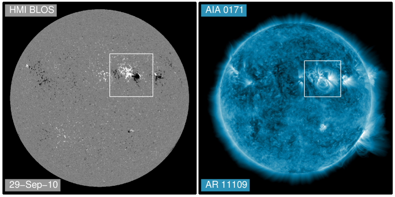
Figure 1: Left: SDO/HMI line-of-sight magnetogram. Right: SDO/AIA 171 Å image. Both images are from 29 September 2010 at 23:21:34. The box in each image shows the patch around active region 11109 selected for the magnetic field extrapolations.

The objective of this paper is to assess how well these existing extrapolation methods reproduce the observed topology of the corona. A future paper will focus on comparing the properties of transient heating events to the properties of the underlying field lines.

This paper is structured in the following way. In Section 2 we provide a brief overview of the different magnetic field extrapolation methods and the field line calculations. In Section 3 we describe the loop tracing and the methods for matching traced loops to field lines. The results from applying this methodology to over 12,000 loops sampled from the 15 active regions is presented in Section 4. A summary and discussion, including a discussion of possible improvements to both the extrapolation methods and loop identification, are presented in Section 5.

2 Magnetic Field Extrapolations

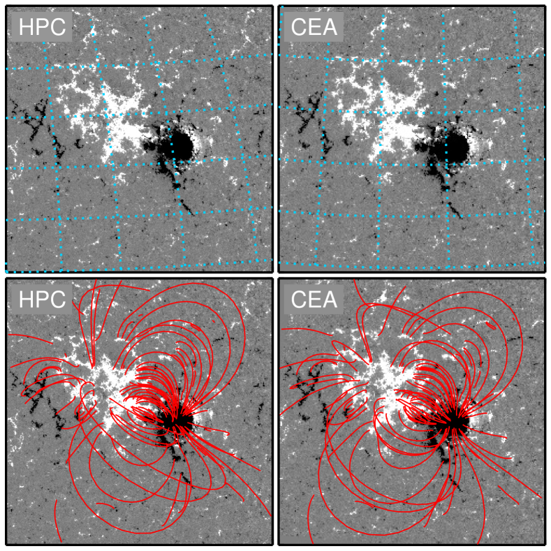
Figure 2: HMI line-of-sight magnetogram patch for active region 11109 on 29 September 2010. Top left: the native magnetogram in helioprojective Cartesian coordinates (HPC). Top right: the magnetogram transformed into the cylindrical equal-area projection (CEA). Lines of heliographic latitude and longitude are shown in each of the top images. Bottom right: field lines from the potential field extrapolation computed in the CEA coordinates and overplotted on the CEA image. Bottom left: the same field lines projected back onto the native HPC magnetogram.

2.1 Potential Field Extrapolation

A potential extrapolation is a solution to the equations

$$\nabla\times\mathbf{B}=0,\quad\nabla\cdot\mathbf{B}=0$$ (1)

using the corrected line of sight component of the observed magnetic field as the lower boundary condition. Introducing the scalar potential $\mathbf{B}=\nabla\varphi$ reduces this to solving Laplace’s equation, $\nabla^{2}\varphi=0$. For this work we use a modified version of a solver based on Fourier transforms (e.g., Alissandrakis, 1981) that we have used in previous studies (e.g., Warren & Winebarger, 2006; Ugarte-Urra et al., 2007, 2017). One of the modifications for this work is to project the observed field from the helioprojective Cartesian (HPC) coordinate system in which the data are taken to a cylindrical equal area (CEA) coordinate system Sun (2013) provides additional details on the transformations to and from a CEA projection. This corrects for foreshortening in the observed magnetograms. See Figures 1 and 2 for an example of such a projection applied to an observation. Previously we had considered regions close to disk center where foreshorting effects are smaller. We also pad the perimeter so that field lines close locally rather than connecting to sources in “adjacent” regions of the periodic domain. This calculation yields the magnetic field components on a Cartesian grid in the CEA coordinate system. We typically use a grid spacing of about $0.1^{\circ}$ per pixel or about $1.8\arcsec$ per pixel and extrapolate up to a height equal to a box side, typically several hundred arc-seconds. A typical calculation takes about 60 s on a standard workstation.

2.2 Wiegelmann Non-Linear Force Free

A non-linear force-free magnetic field is a solution to the equations

$$\nabla\times\mathbf{B}=\frac{4\pi}{c}\mathbf{J}=\alpha\mathbf{B},\quad\nabla\cdot\mathbf{B}=0,$$ (2)

so that $\mathbf{J}\times\mathbf{B}=0$. The twist parameter $\alpha$ is constant along each field line, but varies from field line to field line. As mentioned previously, the lower boundary condition is derived by preprocessing the observed photospheric vector field measurements to make them more consistent with the force-free assumption (Wiegelmann et al., 2006). The preprocessing attempts to find a modified version of the field that is free of forces and torques, is relatively smooth, but is also close to what is observed. The field components at each point are determined by starting with the observations and using gradient descent to find the optimal balance between the four conditions, given a set of relative weights specified by the user.

Once the boundary conditions are determined, the field components are determined by minimizing a functional that is the sum of the squares of the terms in Equation 2 and an error term (see Wiegelmann et al. 2012 Equation 4). As with the potential extrapolation, the NLFF uses the observed photospheric field projected into a CEA coordinate system (see Sun, 2013, for details on the projection of the vector components). We use a resolution of about $0.06^{\circ}$ per pixel or about $1.0\arcsec$ per pixel and extrapolate up to a height of about $160\arcsec$. A typical calculation takes about 6 hours on a standard workstation.

2.3 Aschwanden Vertical Current Forward Fit

The VCA-NLFF method of Aschwanden (2016) uses the radial component of the observed magnetic field as the lower boundary condition and assumes that the field can be represented as a linear superposition of sub-photospheric sources of the form

$$B_{r} = B_{0}\left(\frac{d^{2}}{r^{2}}\right)\frac{1}{1+b^{2}r^{2}\sin^{2}\theta},$$ (3)

$$B_{\phi} = B_{0}\left(\frac{d^{2}}{r^{2}}\right)\frac{br\sin\theta}{1+b^{2}r^{2}\sin^{2}\theta},$$ (4)

$$B_{\theta} = 0,$$ (5)

where $(r,\theta,\phi)$ are spherical coordinates centered at the magnetic source and $d$ is the depth below the photospheric surface. The parameter $b$ is related to the twist of the field by

$$\alpha=\frac{2b\cos\theta}{(1+b^{2}r^{2}\sin^{2}\theta)}.$$ (6)

Note that this representation for the magnetic field is force-free and divergence-free to second order (in the parameter $\alpha$ or $b$, for small values of $\alpha$ or $b$). It is analytically shown that the VCA-NLFFF approximation is exactly divergence-free and force-free in the vertical loop segments near the loop axis above each buried magnetic charge (see Aschwanden 2013a Section 3.3).

The twist parameters for the magnetic sources are iteratively adjusted to minimize the misalignment angle defined in Section 3.3, that is, to provide the best match between the local magnetic field vector and the loops traced in coronal images. Note that to determine the position of the observed loop in three-dimensional space, which is necessary to compute the magnetic field vector, the loop is fit as a circular loop segment, which drives the optimization of the alpha values in the final computed field lines. It is not compared with a computed field line. Also, the loops that we use to tune the parameters in the VCA-NLFF method and the loops that we use to benchmark it are derived from the same procedure (the OCCULT code). We will return to these issues in the next sections.

The resulting extrapolation yields the radial and azimuthal components of the field. These vector components are transformed to Cartesian coordinates, which is consistent with the outputs of the other codes. This method rebins the input magnetogram to a resolution of about $1.5\arcsec$ per pixel and extrapolates up to a height of several hundred arc-seconds. A typical calculation takes about 10 minutes to converge on a standard workstation. The VCA-NLFF code is written in IDL and distributed through SolarSoftWare (SSW, Freeland & Handy 1998).

2.4 Computing Field Lines

Each of the extrapolation techniques yields the components of the magnetic field in a Cartesian coordinate system. Thus the field lines are determined by

$$\frac{ds}{B}=\frac{dx}{B_{x}}=\frac{dy}{B_{y}}=\frac{dz}{B_{z}},$$ (7)

which we integrate using a fourth-order Runge-Kutta method with adaptive step size (Press et al., 1992). To accelerate the calculation of field lines we have written this code in C.

For the potential and vector NLFF methods we need to project the field lines computed in the CEA coordinate system back to the helioprojective Cartesian coordinate system of the original image. This transformation is a multi-step process. We first transform $(x_{cea},y_{cea})$ to heliographic latitude and longitude $(\theta,\varphi)$ and then extend these coordinates to Stonyhurst heliographic coordinates $(r,\theta,\varphi)$ assuming $r=R_{\odot}+z_{cea}$. These coordinates are then transformed to helioprojective-Cartesian, which accounts for the apparent latitude (B-angle) and longitude of the observation at Earth (see Equation 11 of Thompson 2006). An example of this mapping of field lines from CEA to HPC is shown in Figure 2. The transformation from the three-dimensional Cartesian box of the extrapolation to the spherical geometry of the sun is not unique and introduces unavoidable distortions that increase with height away from the surface. The VCA-NLFF extrapolation is computed in Stonyhurst coordinates, so only the final transformation to helioprojective-Cartesian coordinates is needed to map field lines back to the image plane. Finally, we note that the image time need not be close to the time of the magnetogram used for the extrapolation. It is a simple matter to rotate the coordinates of the field lines in heliographic coordinates.

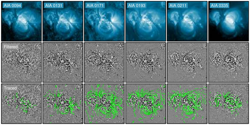
Figure 3: An example of observed coronal loops identified using automated loop tracing on AIA images from AR 11109. The top row shows a 8-image average for each AIA channel used. Images in the middle row are high-pass/low-pass filtered to identify high signal-to-noise features. Automatically identified loop segments from each image are displayed in green in the bottom row.

3 Comparison to Coronal Loops

3.1 Automated Loop Identification

To make systematic comparisons between many loops traced in coronal images and the field lines computed from the magnetic field extrapolations, we must use an automated loop tracing algorithm. Methods for comparing field lines to observed coronal structures without explicitly tracing the loops have been developed (e.g., Carcedo et al., 2003; Conlon & Gallagher, 2010), but these approaches require user inputs for each case. For our work we use the Oriented Coronal CUrved Loop Tracing (OCCULT) code described in Aschwanden (2010) and Aschwanden et al. (2013). The first step in this algorithm is to compute the difference between lowpass and highpass filtered versions of an image. This eliminates both the large-scale background and noise. The second step is to trace along the intensity ridge emanating from the brightest point in the image. After a loop is identified, the pixels in the image associated with it are set to zero and the process is repeated.

The OCCULT code is used in the VCA-NLFF algorithm to identify loop segments. We, however, also run it as a separate module on data that we have processed independently. The VCA code automatically downloads a single, full-disk AIA image for each wavelength of interest. We found that by downloading a time sequence of AIA cutouts for the region of interest and averaging them together we are able to identify a larger number of loops. Loops traced in the averaged images also tend to be longer and appear to be more complete. An example of loops traced on a set of 6 AIA EUV images from AR 11109 is shown in Figure 3.

3.2 Mapping Field Lines to Traced Loops

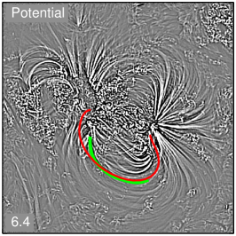
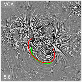
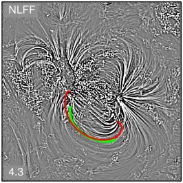
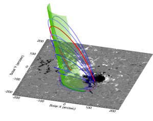
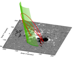
Figure 4: Best-fit field lines for an observed loop in active region 4. Top panels: an observed coronal loop (green) in AIA 171 Å along with the best-fit field line (red) from each extrapolation. The mean minimum distance values are given in the lower left corner of each image. Bottom left panel: To find the best-fit field line we project the traced loop back to the coordinate system of the extrapolation assuming a range of possible heights. Here we show the potential case. This projection forms a surface or “curtain” (shown in light green), which is used to generate seed points for computing candidate field lines (shown in blue). The candidate field lines are projected onto the image plane for comparison with the traced loop. The field line that produces the smallest mean distance is considered to be the best-fit field line (shown in red). This process is repeated for all three extrapolations. Bottom right panel: The best-fit field lines from the three extrapolations plotted in the CEA coordinate system.

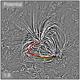
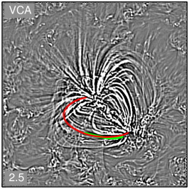
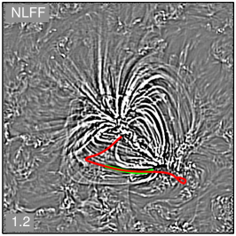
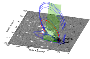
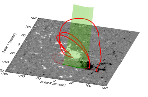
Figure 5: Same as Figure 4 for a loop in active region 1. This example illustrates the differences in the magnetic field topology produced by the three models.

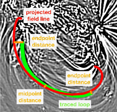
Figure 6: An example of a mean minimum distance calculation with $N=3$. The shortest distance between the endpoints and the midpoint of the traced loop (shown in green) and any point on the projected field line (shown in red) are averaged. This metric is used to evaluate how closely projected field lines match traced loops. For this work we scale $N$ with loop length and between 4 and 50 points are considered.

The final element of this program is a method for matching each traced loop in the AIA images to a field line computed from the extrapolated magnetic field. As mentioned previously, the principal problem is that the traced loops are projected onto the image plane and the three dimensional geometry of the loop is ambiguous. To overcome this we map the 2D coordinates of the traced loop back to the 3D geometry of the extrapolation assuming a range of possible heights. This maps the one dimensional traced loop to a two dimensional, curtain-like surface. Points on this surface are then used as initial conditions for calculating field lines. These field lines are then projected back onto the image plane where they can be compared with the traced loop. Examples of this calculation are shown in Figures 4 and 5.

To determine how well matched a given field line is to a traced loop, we compute the average of the minimum Euclidean distance between several points on the traced loop and the field line. We refer to this average as the “mean minimum distance.” Mathematically this is

$$\mathrm{Mean\ Minimum\ Distance}=\frac{1}{N}\sum_{i=1}^{N}d_{min}(s_{i},s^{\prime}),$$ (8)

where $d_{min}(s_{i},s^{\prime})$ is the minimum distance between a point on the traced loop ($s_{i}$) and any point on the projected field line ($s^{\prime}$). Here we consider a number of points on the traced loop as a function of loop length. We use 1 point for every $4\arcsec$ of loop length, which gives about 50 points for the longest loops and 4 points for the shortest loops. An example calculation illustrating the distances to the two endpoints and the midpoint of the traced loop is shown in Figure 6. A very similar metric was used by Savcheva & van Ballegooijen (2009) for comparing flux rope models with soft X-ray images of sigmoids.

By computing the mean minimum distance for each of the candidate field lines we are able to identify the best-fit or closest field line from the extrapolation for each loop segment. The field, of course, is continuous and we can only sample it discretely. To increase the probability that we find the best possible match we have implemented the following procedure for sampling the domain. We randomly sample 2000 points on the curtain to use as seeds for computing initial field lines. We then choose the best 10 field lines that provide the closest match and consider points that are slightly perturbed away from the seeds of this first batch. From this we generate a second batch of candidate field lines and then select the best-fit from all candidates. In total we consider 4,000 field lines per traced loop. We have tested this procedure by manually tracing out projected field lines and supplying them to the algorithm as if they were traced loops. The mean minimum distance metric for these test loops is typically less than 1″and the best-fit field line is always close to the input field line.

One important issue is that the loop tracing does not necessarily return complete loops. Most traced loops are likely to be only a loop segment sampled from a longer loop. Even if the algorithm does manage to trace out a complete loop, we wouldn’t necessarily be certain of this and be able to add further constraints on the location of the field line footpoints. Thus it is easy to imagine scenarios where the closest matched field line is not really related to the traced loop. A long, overlying field line, for example, could be matched to a small loop segment that actually lies close to the solar surface. Unfortunately, it is not obvious how to resolve this limitation. Some ideas will be discussed in the final section of the paper.

3.3 Misalignment Angle

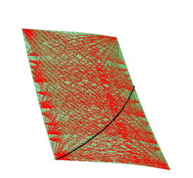
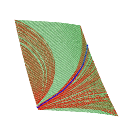
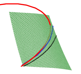
Figure 7: An example of a misalignment angle calculation. Here test geometries are traced across the surface of points that project back to the traced loop (this is the example from Figure 4) and the geometry with the smallest misalignment angle is chosen to represent the loop in 3D. Left panel: The 180 test geometries assumed in the VCA model. The geometry with the smallest median misalignment angle is indicated in black. Center panel: Test geometries generated by following paths of minimum misalignment angle across the surface. The geometry with the smallest median misalignment angle is indicated in blue. Right panel: Comparison of the geometries derived from the misalignment angles with the best-fit field line derived from the distance metric, which is shown in red.

Another point of comparison between traced loops and the magnetic field is the misalignment angle, that is, the angle between the vector formed by two points on the traced loop segment and the local magnetic field vector. For a field line the angle between $\mathbf{B}$ and $\mathbf{ds}$ is zero by construction. If the misalignment angle is large, magnetic field lines will quickly diverge away from the traced loop and the field is a poor representation of the loop geometry.

For stereoscopically observed loops the three dimensional position of the loop is known and this quantity is a very useful measure of how well the field represents the loop. De Rosa et al. (2009), for example, computed the misalignment angle for several active region loops imaged from multiple vantage points and found that none of the NLFF extrapolations could improve on the mean misalignment angle of the potential model ($\sim 24^{\circ}$).

The VCA model is optimized using the misalignment angle, so this metric is also important to compute for our study, even though the loops are observed only as two-dimensional projections. For this case the three dimensional geometry of the loop must be estimated. This is done by assuming a wide variety of parameterized functions for $h(s)$, the variation of height with distance along the traced loop segment (see Figure 11 in Aschwanden 2016). The misalignment angle is computed for each of these parameterizations and the one with the smallest median angle is selected to represent the traced loop. An example of this calculation is shown in Figure 7.

The VCA model assumes that the 3D geometry of the loop is circular. It is possible to remove this restriction by selecting a point on the edge of the curtain and, as is illustrated in Figure 7, following the path of minimum misalignment angle across it. The curve with the smallest median angle is selected to represent the traced loop. Curves which do not cross the curtain are excluded. For a small number of cases no curves that cross the curtain are found. Test calculations suggest that this method produces 3D loop geometries that more closely match the best-fit field lines than the circular assumption does, and we compute misalignment angles using both methods.

We note that the misalignment angle calculation and the mean minimum distance calculations are closely related. The mean minimum distance calculation finds the field line that is the closest match to the loop observed on the image plane. The misalignment angle calculation finds the 3D loop geometry that matches the traced loop in 2D and is most like a field line.

4 Results

Table 1: Active Region Summary

Region	NOAA	Date	$X_{cen}$	$Y_{cen}$	$X_{fov}$	$Y_{fov}$
1	11082	19-Jun-2010 01:27:42	-308.8	470.8	322	322
2	11082	21-Jun-2010 01:16:27	112.9	423.1	392	392
3	11089	23-Jul-2010 14:32:56	-380.5	-437.9	402	402
4	11109	29-Sep-2010 23:21:34	340.9	245.9	462	462
5	11147	21-Jan-2011 13:40:56	-61.3	470.7	502	502
6	11150	31-Jan-2011 10:55:11	-587.7	-258.0	392	392
7	11158	12-Feb-2011 15:01:57	-306.2	-206.8	352	352
8	11187	11-Apr-2011 11:30:35	-530.3	283.3	512	512
9	11190	15-Apr-2011 00:47:05	190.5	307.5	492	492
10	11193	19-Apr-2011 13:02:06	-13.7	372.0	492	492
11	11243	02-Jul-2011 03:08:12	-357.2	167.9	372	372
12	11259	25-Jul-2011 09:05:57	180.9	324.3	322	322
13	11271	21-Aug-2011 11:56:09	-48.7	133.1	552	552
14	11339	08-Nov-2011 18:44:44	51.0	246.0	552	552
15	11339	10-Nov-2011 11:03:29	374.9	256.1	482	482

We have described all of the elements that are needed to carry out this study. We have three different methods for computing the magnetic field components, we can compute field lines and map them back and forth between the computational domain and the image plane, we can automatically trace out loops in coronal images, we have a method for matching field lines to traced loops as well as methods for estimating the misalignment angle. We now turn to the application of this methodology to an ensemble of active regions.

For this study we use the 15 active regions from Warren et al. (2012), who used these regions to study the dependence of active region temperature structure on the properties of the magnetic field. These regions cover about an order of magnitude in the total unsigned magnetic flux, $4\times 10^{21}$ – $3\times 10^{22}$ Mx., covering almost the full range of typically observed active regions. Information on these regions is listed in Table 1. Note that the times correspond to the midpoints of raster observations with the EUV Imaging Spectrometer on Hinode (EIS, Culhane et al. 2007). For each region we have manually selected a field of view that includes all of the flux from the active region core (see Figure 1). Using the field of view and time we downloaded cutouts from the SDO Joint Science Operations Center for a one hour interval beginning with the time listed in the table. The downloads included all of the AIA EUV channels (171, 193, 211, 335, 94, 131, 304) at 12 s, cadence, the AIA UV channels (1600, 1700) at 24 s cadence, the HMI line of sight magnetograms at 45 s cadence, and the HMI vector data at 720 s cadence. As noted earlier, the VCA-NLFF code independently downloads single, full-disk AIA EUV and HMI line-of-sight images.

Table 2: Summary of Loop Comparisons

	Minimum Distance					Misalignment Angle (circular)					Misalignment Angle (arbitrary)
Wavelength	N Loops	PFE	VCA	NLFF		N Loops	PFE	VCA	NLFF		N Loops	PFE	VCA	NLFF
All	12202	1.45	1.72	0.70		12202	11.7	11.4	12.3		11779	5.2	5.4	4.8
94	582	1.11	1.25	0.55		582	11.5	10.6	11.9		568	5.2	4.6	4.5
131	1357	1.20	1.52	0.63		1357	10.5	9.9	11.3		1318	4.6	4.8	4.5
171	2759	1.64	1.92	0.80		2759	11.4	10.8	12.1		2634	5.1	5.5	4.8
193	3224	1.57	1.89	0.73		3224	12.1	12.2	12.9		3115	5.5	5.8	4.9
211	2997	1.50	1.79	0.70		2997	12.2	12.1	12.8		2889	5.4	5.6	4.9
335	1283	1.15	1.29	0.58		1283	11.8	10.9	11.9		1255	5.1	4.9	4.5
Hot	214	1.46	1.31	0.61		214	13.2	11.7	13.0		214	6.2	6.1	4.9

For each region we computed the potential, NLFF, and VCA-NLFF magnetic field extrapolations and saved the field components to a file. Example field line calculations for each region are shown in Figures 9–11. Note that in these plots randomly selected field lines are shown, they have not been matched to any traced loops. Also, field lines for the same randomly selected seed points are shown in each row.

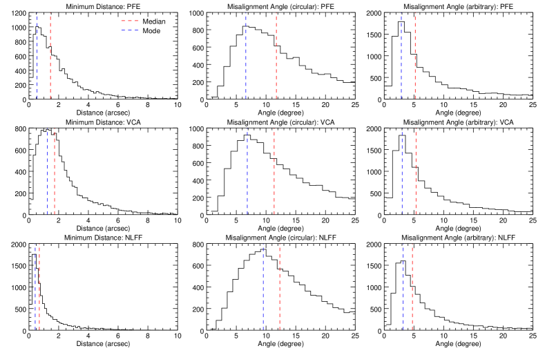
Figure 8: Distributions of minimum distances and misalignment angles for the three extrapolation methods. In general, the differences among the distributions are small. The distance metric for the vector NLFF shows the closest matches and has the narrowest distribution.

For each region we traced loops in the AIA 94, 131, 171, 193, 211, and 335 images. A total of 12,202 loop segments were identified. The loop segments range in projected length from 17″ to about 200″. The distribution of loop lengths is a power law with an index of approximately 3, consistent with Aschwanden et al. (2013). As is evident in Figure 3, the majority of the loop segments are identified in the 171, 193, and 211 channels. These channels generally show emission from ions formed at about 1 MK and thus these comparisons are heavily weighted towards loops at this temperature.

As mentioned in Section 3.1, we have identified loop segments independently of the VCA-NLFF algorithm, but there is some overlap. Of the 12,202 loop segments from our sample, only 2,613 (about 21%) were also used in optimizing the VCA-NLFF model parameters, and thus a large fraction of the loops used to evaluate its performance are independent of the training data.

We computed the mean minimum distance metric for each traced loop for each of the extrapolations. The result of this calculation is summarized in Table 2, where we present median values for all of the loops and for the loops in each AIA wavelength individually. For this metric, the NLFF extrapolation indicates better fits than both the potential and VCA models. This is true for both the aggregate value and for each AIA wavelength considered individually.

As discussed previously, the VCA method is optimized using the misalignment angle and we also computed this metric for each traced loop for each of the three extrapolations. As indicated in Table 2, the VCA yields smaller misalignment angles than either the potential or NLFF methods, although the differences are generally small. This calculation assumes that the 3D loop segments are circular. If we relax the assumption of circular loop segments and consider 3D loop segments that follow paths that minimize the misalignment angle (see Figure 7), the median misalignment angle is reduced and the NLFF extrapolation yields the smallest values.

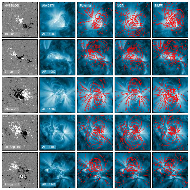
Figure 9: Comparison of extrapolation results. HMI and AIA observations are shown for the active regions in this study along with the resulting field lines from each extrapolation. Field lines are computed using common seed points and projected onto the AIA 171 Å image. Note that these field lines are selected randomly and do not correspond to traced loops. Active regions 1–5 are shown.

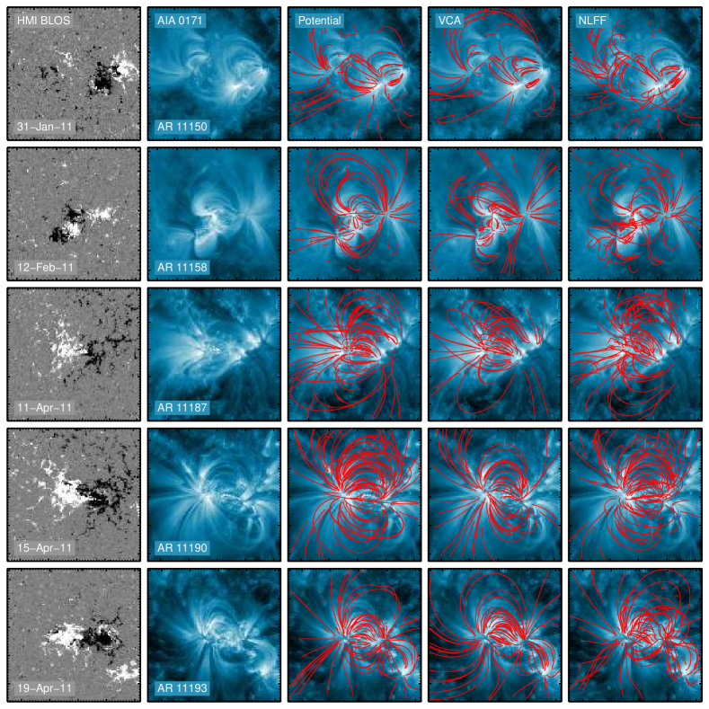
Figure 10: Same as Figure 9 for active regions 6–10.

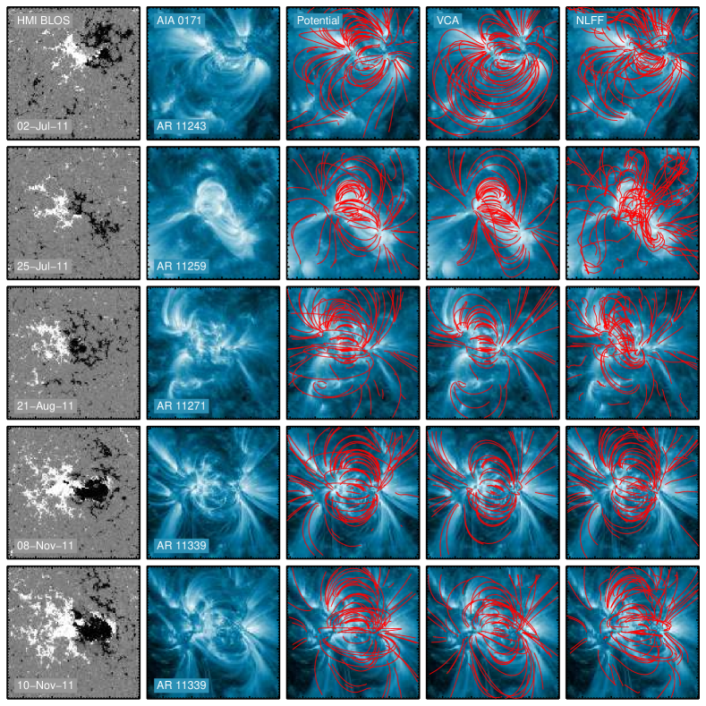
Figure 11: Same as Figure 10 for active regions 11–15.

We have also examined the distributions of distances and misalignment angles for each of the extrapolations. As is shown in Figure 8, these distributions are not Gaussian, but resemble log-normal or power-law distributions. Thus the median and the mode of each distribution are not the same. The general trends, however, are consistent with the results summarized in Table 2. The smallest deviations and the narrowest distribution is for the distance metric applied to the vector NLFF extrapolation. The other metrics and extrapolation techniques generally yield similar results.

The values that we obtain for the misalignment angle are about a factor of two smaller then what was presented by De Rosa et al. (2009) for a set of stereoscopically observed loops. Since we obtain a consistent misalignment angle of $\approx 10^{\circ}$–$13^{\circ}$, independent of the active region, observed wavelength, or magnetic field code (PFE, VCA, NLFF), as well as the consistency of the misalignment angles found in other studies (see Aschwanden et al. 2016 Table 3), we conclude that the smaller misalignment angle that we find in this study is not due to a data selection effect, but rather a limitation of the stereoscopic triangulation method using STEREO data. STEREO has a much poorer spatial resolution (pixel size or 1.59″ and spatial resolution of $\approx 4.0$″) than AIA (0.6″ pixel size and spatial resolution of $\approx 1.5$″). The stereoscopic error itself was determined to be of order $7.6^{\circ}$–$11.5^{\circ}$ (Table 2 in Aschwanden & Sandman 2010). This leads to misalignment angles of $19^{\circ}\pm 3^{\circ}$ for the 3D-misalignment angle (Table 3 in Aschwanden 2013b), or $14.3^{\circ}$–$19.2^{\circ}$ (Section 3.3 in Aschwanden et al. 2012a). Thus, magnetic field modeling with AIA data yields typical misalignment angles of $\approx 10^{\circ}$, while stereoscopically triangulated loops using STEREO data produce a misalignment angle that is about a factor of 2 larger.

To further explore the bias towards potential loops imaged in the AIA 171, 193, and 211 channels we have attempted to isolate loops associated with high-temperature emission. To do this we have processed the AIA 94 images to remove the contribution from million-degree plasma and isolate the emission from the Fe XVIII 93.92 Å line, which is formed at about 7 MK (see Warren et al. 2012 for details). We re-ran the loop tracing algorithm on these processed images and identified a new set of hot loops. We then matched these loops to the loops from our original ensemble that used the unprocessed images. Visual inspection shows that these hot loops are preferentially found in the active region core.

The results from these hot loops are summarized in the final row of Table 2. As expected, for this population of hot loops the potential extrapolation is outperformed by the NLFF methods in all metrics. The differences, however, are not particularly large. Unfortunately, we are able to identify only 214 hot loops in our sample of 12,202 total loops.

5 Summary and Discussion

We have presented systematic comparisons between magnetic field lines computed from three different extrapolation methods and the topology of coronal loops inferred from AIA images. The NLFF methods generally provide better matches between the field and the observed loops. The NLFF method based on vector data yields the smallest values for the distance metric. The VCA and NLFF methods yield smaller values for the misalignment angle than the potential. The differences, however, are generally small: about 1″ for the distance metric and about 1^∘ for the misalignment angle. A visual inspection of the best-fit field lines, such as those presented in Figures 4 and 5, also suggest relatively small differences between the different extrapolation methods.

This study highlights some fundamental limitations of the available data and extrapolation methods. Improvements in these areas should lead to better fits between the extrapolations and the observed loops.

High Temperature Emission

As noted earlier, the majority of the identified loops are from emission formed at a about 1 MK. The currents are likely to be strongest along the neutral line in the active region core, where loops generally have much higher temperatures. Studies with Hinode/EIS have shown that these loops are generally about 4 MK (Warren et al., 2011, 2012; Del Zanna, 2013). The AIA 94 channel includes Fe XVIII, but this is formed at about 8 MK and strong Fe XVIII emission is generally only observed in large active regions or in transient heating events. When Fe XVIII emission is observed, loop identification may be improved if the AIA 94 images are processed to remove the contribution from lower temperature emission (see Warren et al. 2012; Teriaca et al. 2012a).

It is likely that observations from the X-ray Telescope on Hinode (XRT, Golub et al. 2007) could be used for identifying high temperature loops. As mentioned previously, Savcheva & van Ballegooijen (2009) used XRT images to constrain a NLFF model of a sigmoid, but selected the observed loops manually. However, the broad temperature response of XRT may limit the efficacy of the automated loop tracing.

High spatial resolution observations of emission lines formed at about 4 MK, such as Ca XIV 193.874 Å, would be ideal for identifying the topology of loops in the active region core. Such an instrument is being considered for a future Japanese space mission (e.g., Teriaca et al. 2012b).

Chromospheric Emission

Matching chromospheric structures observed at high spatial resolution with IRIS or a ground-based observatory is a complementary approach to studying non-potential fields in the core of the active region. Since such data is not available for all of the active regions considered here, we have not pursued this idea here. The limited field of view for high resolution data are also an obstacle to applying such data to this problem. Aschwanden et al. (2016) has done exploratory calculations for three active regions and was able to find good agreement between the VCA model and loops traced at chromospheric temperatures near a sunspot.

Projection Effects

Coronal images show projections of three dimensional structures onto a two dimensional plane, which limits our ability to compare loops traced in coronal images and field lines. As we have seen, to project traced loops back to three dimension space involves many assumptions about the field line geometry. Projecting field lines onto the image plane does not involve any assumptions, but since we cannot be sure that we are comparing with a complete loop, it does not yield a unique result.

Observations from multiple viewing angles are an obvious solution to this problem and the STEREO (Kaiser et al., 2008) mission has provided several examples of this (e.g., Aschwanden et al., 2012c, b; Aschwanden, 2013b; Chifu et al., 2015, 2017). Unfortunately, stereoscopic observations have been very limited and are not likely to be taken routinely in the near future. Solar Orbiter (Müller et al., 2013) will take coronal images from vantage points away from the Sun-Earth line, but the launch of this mission is still several years away.

One possibility for reducing projection ambiguities is to consider time sequences of images rather than individual snapshots. The time sequences would allow transient brightenings to be detected. Since it is likely that the brightening occurs over the entire loop, this would provide the full loop geometry. This constrains the search space for potential field line matches considerably. We are currently investigating this approach using observations from the AIA 94 channel.

Preprocessing

Chifu et al. (2017) extended the NLFFF optimization code by implementing the additional constraint to minimize the angle between the reconstructed local magnetic field direction and the orientation of 3D-loops. In that study a number of 3D-loops have been stereoscopically reconstructed from EUV-images from three vantage points (STEREO A, B and SDO). The method was dubbed S-NLFFF. While in the current implementation the method requires 3D- loops to constrain the NLFFF-code, a generalization towards using traced 2D-loops from one image is ongoing work.

Metrics

We have considered two metrics for comparing field lines to observed loops, the minimum distance and the misalignment angle. When only 2D projected loop observations are available, the minimum distance metric is likely to be the most useful. This metric identifies the topological feature of interest (the field line) using the observations directly and avoids the intermediate step of estimating the 3D loop geometry. Future studies involving 2D observations should use this metric along with the misalignment angle.

References

- Alissandrakis (1981) Alissandrakis, C. E. 1981, A&A, 100, 197
- Amari et al. (2006) Amari, T., Boulmezaoud, T. Z., & Aly, J. J. 2006, A&A, 446, 691, doi: 10.1051/0004-6361:20054076
- Aschwanden et al. (2013) Aschwanden, M., De Pontieu, B., & Katrukha, E. 2013, Entropy, 15, 3007, doi: 10.3390/e15083007
- Aschwanden (2010) Aschwanden, M. J. 2010, Sol. Phys., 262, 399, doi: 10.1007/s11207-010-9531-6
- Aschwanden (2013a) —. 2013a, Sol. Phys., 287, 323, doi: 10.1007/s11207-012-0069-7
- Aschwanden (2013b) —. 2013b, ApJ, 763, 115, doi: 10.1088/0004-637X/763/2/115
- Aschwanden (2016) —. 2016, ApJS, 224, 25, doi: 10.3847/0067-0049/224/2/25
- Aschwanden & Malanushenko (2013) Aschwanden, M. J., & Malanushenko, A. 2013, Sol. Phys., 287, 345, doi: 10.1007/s11207-012-0070-1
- Aschwanden et al. (2016) Aschwanden, M. J., Reardon, K., & Jess, D. B. 2016, ApJ, 826, 61, doi: 10.3847/0004-637X/826/1/61
- Aschwanden & Sandman (2010) Aschwanden, M. J., & Sandman, A. W. 2010, AJ, 140, 723, doi: 10.1088/0004-6256/140/3/723
- Aschwanden et al. (2012a) Aschwanden, M. J., Wuelser, J.-P., Nitta, N. V., et al. 2012a, ApJ, 756, 124, doi: 10.1088/0004-637X/756/2/124
- Aschwanden et al. (2012b) —. 2012b, ApJ, 756, 124, doi: 10.1088/0004-637X/756/2/124
- Aschwanden et al. (2012c) Aschwanden, M. J., Wülser, J.-P., Nitta, N., & Lemen, J. 2012c, Sol. Phys., 281, 101, doi: 10.1007/s11207-012-0092-8
- Bradshaw & Viall (2016) Bradshaw, S. J., & Viall, N. M. 2016, ApJ, 821, 63, doi: 10.3847/0004-637X/821/1/63
- Carcedo et al. (2003) Carcedo, L., Brown, D. S., Hood, A. W., Neukirch, T., & Wiegelmann, T. 2003, Sol. Phys., 218, 29, doi: 10.1023/B:SOLA.0000013045.65499.da
- Chifu et al. (2015) Chifu, I., Inhester, B., & Wiegelmann, T. 2015, A&A, 577, A123, doi: 10.1051/0004-6361/201322548
- Chifu et al. (2017) Chifu, I., Wiegelmann, T., & Inhester, B. 2017, ApJ, 837, 10, doi: 10.3847/1538-4357/aa5b9a
- Conlon & Gallagher (2010) Conlon, P. A., & Gallagher, P. T. 2010, ApJ, 715, 59, doi: 10.1088/0004-637X/715/1/59
- Culhane et al. (2007) Culhane, J. L., Harra, L. K., James, A. M., et al. 2007, Sol. Phys., 243, 19, doi: 10.1007/s01007-007-0293-1
- De Pontieu et al. (2014) De Pontieu, B., Title, A. M., Lemen, J. R., et al. 2014, Sol. Phys., 289, 2733, doi: 10.1007/s11207-014-0485-y
- De Rosa et al. (2009) De Rosa, M. L., Schrijver, C. J., Barnes, G., et al. 2009, ApJ, 696, 1780, doi: 10.1088/0004-637X/696/2/1780
- Del Zanna (2013) Del Zanna, G. 2013, A&A, 558, A73, doi: 10.1051/0004-6361/201321653
- DeRosa et al. (2015) DeRosa, M. L., Wheatland, M. S., Leka, K. D., et al. 2015, ApJ, 811, 107, doi: 10.1088/0004-637X/811/2/107
- Freeland & Handy (1998) Freeland, S. L., & Handy, B. N. 1998, Sol. Phys., 182, 497, doi: 10.1023/A:1005038224881
- Golub et al. (2007) Golub, L., Deluca, E., Austin, G., et al. 2007, Sol. Phys., 243, 63, doi: 10.1007/s11207-007-0182-1
- Jiang & Feng (2013) Jiang, C., & Feng, X. 2013, ApJ, 769, 144, doi: 10.1088/0004-637X/769/2/144
- Kaiser et al. (2008) Kaiser, M. L., Kucera, T. A., Davila, J. M., et al. 2008, Space Sci. Rev., 136, 5, doi: 10.1007/s11214-007-9277-0
- Kobayashi et al. (2014) Kobayashi, K., Cirtain, J., Winebarger, A. R., et al. 2014, Sol. Phys., 289, 4393, doi: 10.1007/s11207-014-0544-4
- Lemen et al. (2012) Lemen, J. R., Title, A. M., Akin, D. J., et al. 2012, Sol. Phys., 275, 17, doi: 10.1007/s11207-011-9776-8
- Lundquist et al. (2008) Lundquist, L. L., Fisher, G. H., Metcalf, T. R., Leka, K. D., & McTiernan, J. M. 2008, ApJ, 689, 1388, doi: 10.1086/592760
- Malanushenko et al. (2012) Malanushenko, A., Schrijver, C. J., DeRosa, M. L., Wheatland, M. S., & Gilchrist, S. A. 2012, ApJ, 756, 153, doi: 10.1088/0004-637X/756/2/153
- Metcalf et al. (1995) Metcalf, T. R., Jiao, L., McClymont, A. N., Canfield, R. C., & Uitenbroek, H. 1995, ApJ, 439, 474, doi: 10.1086/175188
- Müller et al. (2013) Müller, D., Marsden, R. G., St. Cyr, O. C., & Gilbert, H. R. 2013, Sol. Phys., 285, 25, doi: 10.1007/s11207-012-0085-7
- Press et al. (1992) Press, W. H., Teukolsky, S. A., Vetterling, W. T., & Flannery, B. P. 1992, Numerical Recipes in C (2Nd Ed.): The Art of Scientific Computing (New York, NY, USA: Cambridge University Press)
- Savcheva & van Ballegooijen (2009) Savcheva, A., & van Ballegooijen, A. 2009, ApJ, 703, 1766, doi: 10.1088/0004-637X/703/2/1766
- Scherrer et al. (2012) Scherrer, P. H., Schou, J., Bush, R. I., et al. 2012, Sol. Phys., 275, 207, doi: 10.1007/s11207-011-9834-2
- Schrijver et al. (2004) Schrijver, C. J., Sandman, A. W., Aschwanden, M. J., & De Rosa, M. L. 2004, ApJ, 615, 512, doi: 10.1086/424028
- Sun (2013) Sun, X. 2013, ArXiv e-prints. https://arxiv.org/abs/1309.2392
- Teriaca et al. (2012a) Teriaca, L., Warren, H. P., & Curdt, W. 2012a, ApJ, 754, L40, doi: 10.1088/2041-8205/754/2/L40
- Teriaca et al. (2012b) Teriaca, L., Andretta, V., Auchère, F., et al. 2012b, Experimental Astronomy, 34, 273, doi: 10.1007/s10686-011-9274-x
- Thompson (2006) Thompson, W. T. 2006, A&A, 449, 791, doi: 10.1051/0004-6361:20054262
- Ugarte-Urra et al. (2017) Ugarte-Urra, I., Warren, H. P., Upton, L. A., & Young, P. R. 2017, ApJ, 846, 165, doi: 10.3847/1538-4357/aa8597
- Ugarte-Urra et al. (2007) Ugarte-Urra, I., Warren, H. P., & Winebarger, A. R. 2007, ApJ, 662, 1293, doi: 10.1086/514814
- Valori et al. (2012) Valori, G., Green, L. M., Démoulin, P., et al. 2012, Sol. Phys., 278, 73, doi: 10.1007/s11207-011-9865-8
- Warren et al. (2011) Warren, H. P., Brooks, D. H., & Winebarger, A. R. 2011, ApJ, 734, 90, doi: 10.1088/0004-637X/734/2/90
- Warren & Winebarger (2006) Warren, H. P., & Winebarger, A. R. 2006, ApJ, 645, 711, doi: 10.1086/504075
- Warren & Winebarger (2007) —. 2007, ApJ, 666, 1245, doi: 10.1086/519943
- Warren et al. (2012) Warren, H. P., Winebarger, A. R., & Brooks, D. H. 2012, ApJ, 759, 141, doi: 10.1088/0004-637X/759/2/141
- Wheatland (2007) Wheatland, M. S. 2007, Sol. Phys., 245, 251, doi: 10.1007/s11207-007-9054-y
- Wiegelmann (2004) Wiegelmann, T. 2004, Sol. Phys., 219, 87, doi: 10.1023/B:SOLA.0000021799.39465.36
- Wiegelmann et al. (2006) Wiegelmann, T., Inhester, B., & Sakurai, T. 2006, Sol. Phys., 233, 215, doi: 10.1007/s11207-006-2092-z
- Wiegelmann et al. (2012) Wiegelmann, T., Thalmann, J. K., Inhester, B., et al. 2012, Sol. Phys., 281, 37, doi: 10.1007/s11207-012-9966-z
- Winebarger et al. (2008) Winebarger, A. R., Warren, H. P., & Falconer, D. A. 2008, ApJ, 676, 672, doi: 10.1086/527291
- Xie et al. (2017) Xie, H., Madjarska, M. S., Li, B., et al. 2017, ApJ, 842, 38, doi: 10.3847/1538-4357/aa7415