A general procedure for detector-response correction of higher order cumulants

Abstract

We propose a general procedure for the detector-response correction (including efficiency correction) of higher order cumulants observed by the event-by-event analysis in heavy-ion collisions. This method makes use of the moments of the response matrix characterizing the property of a detector, and is applicable to a wide variety of response matrices such as those having non-binomial responses and including the effects of ghost tracks. A procedure to carry out the detector-response correction of realistic detectors is discussed. In test analyses, we show that this method can successfully reconstruct the cumulants of true distribution for various response matrices including the one having multiplicity-dependent efficiency.

I Introduction

Fluctuations are important observables in relativistic heavy-ion collisions for the search for the QCD critical point and the phase transition to the deconfined medium Asakawa and Kitazawa (2016); Luo and Xu (2017). In particular, non-Gaussianity of fluctuations characterized by the higher order cumulants is believed to be sensitive to these phenomena Ejiri et al. (2006); Stephanov (2009); Asakawa et al. (2009). Active measurements of fluctuation observables have been performed by the event-by-event analyses at RHIC Adamczyk et al. (2014a, b); Adare et al. (2016); Adamczyk et al. (2017), the LHC Abelev et al. (2013); Rustamov (2017), and the NA61 Gazdzicki and HADES Holzmann Collaborations. Future experimental facilities, J-PARC Sako et al. , FAIR Rapp et al. (2011), and NICA Blaschke et al. (2016), will also contribute this subject.

In relativistic heavy-ion collisions, the cumulants of a particle-number distribution are obtained from an event-by-event histogram of the particle number observed experimentally. However, because of the imperfect capability of detectors the experimentally-observed event-by-event histogram is modified from the true distribution, and accordingly their cumulants are also altered by these artificial effects. In the experimental analysis, this effect has to be corrected. In this paper we call this procedure as the detector-response correction.

Compared to standard observables given by expectation values, the detector-response correction of the cumulants higher than the first order is more involved, because the change of a distribution function modifies its cumulants in a non-trivial way Asakawa and Kitazawa (2016). So far, the detector-response correction has been discussed by focusing on the efficiency correction, i.e. the correction for the effects of the loss of particles at the measurement. It has been established that the correction can be carried out if one assumes that the probability that the detector observes a particle (efficiency) is uncorrelated for individual particles. In this case, the detector’s response is described by the binomial distribution Kitazawa and Asakawa (2012); Asakawa and Kitazawa (2016), that we call the binomial model Bialas and Peschanski (1986); Kitazawa and Asakawa (2012); Bzdak and Koch (2012, 2015); Luo (2015a); Kitazawa (2016); Nonaka et al. (2016, 2017). Recently, using the method proposed in Ref. Nonaka et al. (2017), the analysis of the net-proton number cumulants is realized up to sixth order Esha (2017).

The assumption for the binomial model, however, is more or less violated at typical detectors in heavy-ion collisions. First, the multiplicity dependence of the efficiency of realistic detectors Luo (2015b); Adamczyk et al. (2017); Holzmann suggests the existence of the correlations between efficiencies of different particles Bzdak et al. (2016). Even worse, typical detectors sometimes measure ghost tracks, i.e. non-existing particles. The estimate on systematic uncertainty arising from these effects is important for reliable experimental analyses of higher order cumulants.

One of the general procedures for the detector-response correction is the unfolding method D’Agostini (1995); Adye (2011); Garg et al. (2013). This method analyzes the true distribution function from experimental results and knowledge on the detector. Strictly speaking, however, the reconstruction of the true distribution function is an ill-posed problem. The estimate on the systematic uncertainty of the final results is a nontrivial task in this method, and a large numerical cost is required for the iterative analysis to obtain the distribution. Furthermore, the analysis of the distribution itself seems redundant because the cumulants are relevant quantities for many purposes. It is desirable to have a method which enables the analysis of the cumulants directly without using the distribution.

In the present study, we propose a new method to perform the detector-response correction of cumulants directly. In this method, we relate the moments of true and observed distributions without using the distribution explicitly. This method can solve the detector-response correction exactly for a wide variety of detector’s responses; for example, those parametrized by the hypergeometric distribution and the binomial model with fluctuating probability. By introducing an approximation with a truncation this method can also deal with the correction of realistic detectors whose response is estimated only by Monte Carlo simulations. We demonstrate by explicit numerical analyses that the correction by this method can be carried out successfully for non-binomial response matrices and the response matrix representing multiplicity-dependent efficiency.

This paper is organized as follows. In Sec. II, we discuss a general procedure for the detector-response correction. The application of this method to the correction of realistic detectors is then discussed in Sec. III. We perform test analyses of this method in Secs. IV and V: We deal with the exactly solvable cases in Sec. IV, and the multiplicity-dependent efficiency in Sec. V, respectively. The last section is devoted to a summary.

II Detector-response correction

II.1 Problem

Let us first clarify the problem. We consider a measurement of the cumulants of an event-by-event distribution of a particle number $N$, whose probability distribution is given by $P(N)$. In experimental measurements, typical detectors cannot count the particle number $N$ in each event accurately due to the miss of particle observation and miscounting of ghost tracks. Therefore, the observed particle number $n$ by the detector in an event is generally different from the true particle number $N$, and its event-by-event distribution denoted by $\tilde{P}(n)$ is also modified from $P(N)$. The goal of the detector-response correction is to obtain the cumulants of $P(N)$ from experimentally-observed distribution $\tilde{P}(n)$ and the knowledge on the detector.

To deal with this problem, we assume that the probability to observe $n$ particles in an event with the true particle number $N$ depends only on $N$. We denote this probability as ${\cal R}(n;N)$; because ${\cal R}(n;N)$ is a probability, it satisfies $\sum_{n}{\cal R}(n;N)=1$. We refer to ${\cal R}(n;N)$ as the response matrix. Using ${\cal R}(n;N)$, $\tilde{P}(n)$ and $P(N)$ are related with each other as

$$\tilde{P}(n)=\sum_{N}{\cal R}(n;N)P(N).$$ (1)

In this study we consider the detector-response correction with Eq. (1). Here, the response matrix ${\cal R}(n;N)$ contains all information on the property of the detector relevant to this problem. We note that Eq. (1) can describe not only the efficiency loss, but also the effects of the ghost tracks.

Although the detector-response correction of a single-particle distribution is considered in Eq. (1), the correction with multi-particle distributions are usually necessary in heavy-ion collisions Nonaka et al. (2017). In this study, however, we basically concentrate on the single-particle distribution for simplicity. The generalization of the procedure to multi-particle distributions is straightforward as discussed in Appendix A.

II.2 Notation

We denote the $m$th-order moment of $\tilde{P}(n)$ as

$$\mathopen{\hbox{${\langle}$}\mkern 2.0mu\kern-3.49998pt\leavevmode\hbox{${\langle}$}}n^{m}\mathclose{\hbox{${\rangle}$}\mkern 2.0mu\kern-3.49998pt\leavevmode\hbox{${\rangle}$}}=\sum_{n}n^{m}\tilde{P}(n),$$ (2)

while that of $P(N)$ is expressed as

$$\langle N^{m}\rangle=\sum_{N}N^{m}P(N).$$ (3)

The $m$th-order cumulants of these distributions are denoted as $\mathopen{\hbox{${\langle}$}\mkern 2.0mu\kern-3.49998pt\leavevmode\hbox{${\langle}$}}n^{m}\mathclose{\hbox{${\rangle}$}\mkern 2.0mu\kern-3.49998pt\leavevmode\hbox{${\rangle}$}}_{\rm c}$ and $\langle N^{m}\rangle_{\rm c}$, respectively.

II.3 Formal solution

Substituting Eq. (1) into Eq. (2) one finds that the $m$th-order moment of $\tilde{P}(n)$ is given by

$$\mathopen{\hbox{${\langle}$}\mkern 2.0mu\kern-3.49998pt\leavevmode\hbox{${\langle}$}}n^{m}\mathclose{\hbox{${\rangle}$}\mkern 2.0mu\kern-3.49998pt\leavevmode\hbox{${\rangle}$}} =\sum_{N}P(N)\sum_{n}n^{m}{\cal R}(n;N)$$

$$=\sum_{N}P(N)R_{m}(N),$$ (4)

where $R_{m}(N)$ is defined as

$$R_{m}(N)=\sum_{n}n^{m}{\cal R}(n;N).$$ (5)

Because ${\cal R}(n;N)$ with fixed $N$ represents a probability, $R_{m}(N)$ is understood as the moments of ${\cal R}(n;N)$.

We then suppose that $R_{m}(N)$ is expanded as

$$R_{m}(N)=\sum_{j=0}r_{mj}N^{j}.$$ (6)

Substituting Eq. (6) into Eq. (4), one obtains

$$\mathopen{\hbox{${\langle}$}\mkern 2.0mu\kern-3.49998pt\leavevmode\hbox{${\langle}$}}n^{m}\mathclose{\hbox{${\rangle}$}\mkern 2.0mu\kern-3.49998pt\leavevmode\hbox{${\rangle}$}}=r_{m0}+\sum_{j=1}r_{mj}\langle N^{j}\rangle.$$ (7)

Equation (7) is expressed in the matrix form as

$$\left[\begin{matrix}\mathopen{\hbox{${\langle}$}\mkern 2.0mu\kern-3.49998pt\leavevmode\hbox{${\langle}$}}n\mathclose{\hbox{${\rangle}$}\mkern 2.0mu\kern-3.49998pt\leavevmode\hbox{${\rangle}$}}\\ \mathopen{\hbox{${\langle}$}\mkern 2.0mu\kern-3.49998pt\leavevmode\hbox{${\langle}$}}n^{2}\mathclose{\hbox{${\rangle}$}\mkern 2.0mu\kern-3.49998pt\leavevmode\hbox{${\rangle}$}}\\ \vdots\\ \end{matrix}\right]=\left[\begin{matrix}r_{10}\\ r_{20}\\ \vdots\end{matrix}\right]+\bm{R}\left[\begin{matrix}\langle N\rangle\\ \langle N^{2}\rangle\\ \vdots\\ \end{matrix}\right],$$ (8)

with the matrix $\bm{R}=(r_{mj})$. If $\bm{R}$ is a regular matrix, by applying $\bm{R}^{-1}$ to Eq. (8) from left one obtains

$$\left[\begin{matrix}\langle N\rangle\\ \langle N^{2}\rangle\\ \vdots\\ \end{matrix}\right]=\bm{R}^{-1}\left[\begin{matrix}\mathopen{\hbox{${\langle}$}\mkern 2.0mu\kern-3.49998pt\leavevmode\hbox{${\langle}$}}n\mathclose{\hbox{${\rangle}$}\mkern 2.0mu\kern-3.49998pt\leavevmode\hbox{${\rangle}$}}\\ \mathopen{\hbox{${\langle}$}\mkern 2.0mu\kern-3.49998pt\leavevmode\hbox{${\langle}$}}n^{2}\mathclose{\hbox{${\rangle}$}\mkern 2.0mu\kern-3.49998pt\leavevmode\hbox{${\rangle}$}}\\ \vdots\\ \end{matrix}\right]-\bm{R}^{-1}\left[\begin{matrix}r_{10}\\ r_{20}\\ \vdots\end{matrix}\right].$$ (9)

In Eq. (9), the moments of the true distribution $\langle N^{m}\rangle$ are expressed by the experimentally-observed moments $\mathopen{\hbox{${\langle}$}\mkern 2.0mu\kern-3.49998pt\leavevmode\hbox{${\langle}$}}n^{m}\mathclose{\hbox{${\rangle}$}\mkern 2.0mu\kern-3.49998pt\leavevmode\hbox{${\rangle}$}}$ together with the parameters $r_{mj}$ characterizing the property of the detector. Because the cumulants of $P(N)$ are obtained from $\langle N^{m}\rangle$ Asakawa and Kitazawa (2016), the detector-response correction of the cumulants is carried out with Eq. (9).

In this argument, one can use alternative expansions of $R_{m}(N)$ instead of Eq. (6), which lead to the same final result but might lead to an enhancement of numerical stability. This strategy is discussed in Appendix B.

II.4 Exactly solvable models

Although the above argument formally solves the problem of the detector-response correction, Eq. (9) is not quite useful when the matrix $\bm{R}$ is not closed at some order. First of all, the inverse matrix of $\bm{R}$ is not determined in general in this case. Second, even if the inverse matrix were obtained, Eq. (9) requires $\mathopen{\hbox{${\langle}$}\mkern 2.0mu\kern-3.49998pt\leavevmode\hbox{${\langle}$}}n^{m}\mathclose{\hbox{${\rangle}$}\mkern 2.0mu\kern-3.49998pt\leavevmode\hbox{${\rangle}$}}$ up to infinitely higher orders. In realistic situations, however, the moments $\mathopen{\hbox{${\langle}$}\mkern 2.0mu\kern-3.49998pt\leavevmode\hbox{${\langle}$}}n^{m}\mathclose{\hbox{${\rangle}$}\mkern 2.0mu\kern-3.49998pt\leavevmode\hbox{${\rangle}$}}$ accessible with a reasonable statistics are limited typically to $m\lesssim 6$.

When the expansions Eq. (6) are terminated at finite orders, Eq. (9) gives a closed form and provides exact formulas for the detector-response correction. Particularly important examples of ${\cal R}(n;N)$ satisfying this condition are the cases that $R_{m}(N)$ is given by a $m$th-order polynomial, i.e.

$$R_{m}(N)=\sum_{j=0}^{m}r_{mj}N^{j}.$$ (10)

In this case, the matrix $\bm{R}$ in Eq. (8) has a lower-triangular form

$$\bm{R}=\left[\begin{matrix}r_{11}&0&0&\cdots\\ r_{21}&r_{22}&0&\cdots\\ r_{31}&r_{32}&r_{33}&\ddots\\ \vdots&\vdots&&\ddots\end{matrix}\right].$$ (11)

The inverse of a lower-triangular matrix is obtained order-by-order, and $\bm{R}^{-1}$ is also lower triangular. Substituting the lower-triangular form of $\bm{R}^{-1}$ into Eq. (9), one finds that $\langle N^{m}\rangle$ depends only on $\mathopen{\hbox{${\langle}$}\mkern 2.0mu\kern-3.49998pt\leavevmode\hbox{${\langle}$}}n^{l}\mathclose{\hbox{${\rangle}$}\mkern 2.0mu\kern-3.49998pt\leavevmode\hbox{${\rangle}$}}$ for $l\leq m$.

The binomial model with ${\cal R}_{\rm bin}(n;N)=B(n;p,N)$ Asakawa and Kitazawa (2016), with the binomial distribution

$$B(n;p,N)=p^{n}(1-p)^{N-n}\frac{N!}{n!(N-n)!}$$ (12)

corresponds to this case. In fact, all the cumulants of the binomial distribution is proportional to $N$,

$$\langle n^{m}\rangle_{\rm c,binomial}=\xi_{m}(p)N,$$ (13)

where the coefficients $\xi_{m}(p)$ depend only on $p$ Nonaka et al. (2017). Converting Eq. (13) into moments, one immediately finds that $R_{m}(N)$ in this case is given by a $m$th-order polynomial as in Eq. (10). In this case, Eq. (9) reproduces the formulas of the efficiency correction in the binomial model Asakawa and Kitazawa (2016).

Other examples satisfying Eq. (10) are the binomial model but the probability $p$ is fluctuating event by event He and Luo (2018),

$${\cal R}_{\rm G}(n;N)=\int_{0}^{1}dpG(p)B(n;p,N),$$ (14)

where $G(p)$ is a probability distribution satisfying $\int_{0}^{1}dpG(p)=1$. The moments $R_{m}(N)$ of Eq. (14) satisfy Eq. (10) for arbitrary forms of $G(p)$, as discussed in Appendix C. The detector-response correction for ${\cal R}_{\rm G}(n;N)$ thus is handled with Eq. (9) exactly. The beta-binomial distribution, which is obtained by $G(p)={\cal B}(p;a,b)$ with the beta distribution ${\cal B}(p;a,b)$, belongs to this case (see Appendix D).

Another interesting response matrix is the one parametrized by the hypergeometric distribution as

$${\cal R}_{\rm HG}(n;N)=H(n;N,X,Y),$$ (15)

where the hypergeometric distribution $H(n;N,X,Y)$ is defined in Appendix D. As shown in Appendix D, the moments of Eq. (15) is given in the form in Eq. (10). Therefore, the detector-response correction for Eq. (15) is also carried out exactly with Eq. (9).

II.5 Truncation

When the expansion of $R_{m}(N)$ is not closed, one must introduce an approximation to deal with the detector-response correction. A simple approximation is a truncation of the expansion Eq. (6) at $L$th order,

$$R_{m}(N)=\sum_{j=0}^{L}r_{mj}N^{j}.$$ (16)

Using Eq. (16), one obtains a closed formula up to the $L$th order

$$\left[\begin{matrix}\mathopen{\hbox{${\langle}$}\mkern 2.0mu\kern-3.49998pt\leavevmode\hbox{${\langle}$}}n\mathclose{\hbox{${\rangle}$}\mkern 2.0mu\kern-3.49998pt\leavevmode\hbox{${\rangle}$}}\\ \mathopen{\hbox{${\langle}$}\mkern 2.0mu\kern-3.49998pt\leavevmode\hbox{${\langle}$}}n^{2}\mathclose{\hbox{${\rangle}$}\mkern 2.0mu\kern-3.49998pt\leavevmode\hbox{${\rangle}$}}\\ \vdots\\ \mathopen{\hbox{${\langle}$}\mkern 2.0mu\kern-3.49998pt\leavevmode\hbox{${\langle}$}}n^{L}\mathclose{\hbox{${\rangle}$}\mkern 2.0mu\kern-3.49998pt\leavevmode\hbox{${\rangle}$}}\end{matrix}\right]=\left[\begin{matrix}r_{10}\\ r_{20}\\ \vdots\\ r_{L0}\end{matrix}\right]+\bm{R}\left[\begin{matrix}\langle N\rangle\\ \langle N^{2}\rangle\\ \vdots\\ \langle N^{L}\rangle\end{matrix}\right],$$ (17)

where $\bm{R}$ is a $L\times L$ matrix. When $\bm{R}$ is a regular matrix, by applying $\bm{R}^{-1}$ from left Eq. (17) enables one to carry out the detector-response correction up to the $L$th order using the experimental data on $\mathopen{\hbox{${\langle}$}\mkern 2.0mu\kern-3.49998pt\leavevmode\hbox{${\langle}$}}n^{m}\mathclose{\hbox{${\rangle}$}\mkern 2.0mu\kern-3.49998pt\leavevmode\hbox{${\rangle}$}}$ for $m\leq L$.

Of course, this analysis can be justified only when the truncated formula Eq. (16) well reproduces the functional form of $R_{m}(N)$. When ${\cal R}(n;N)$ is given by an analytic form, the effect of the truncation would be estimated analytically. When one considers the response matrices of realistic detectors, they are usually estimated by Monte Carlo simulations such as GEANT Agostinelli et al. (2003), which provide the moments $R_{m}(N)$ with statistical errors. In this case, one may perform fits to $R_{m}(N)$ with Eq. (16). The use of Eq. (17) would be justified as long as these fits reproduce $R_{m}(N)$ within statistics. The detector-response correction of realistic detectors will be discussed in Sec. III in more detail.

III Practical analysis

In this section, we discuss the detector-response correction of realistic detectors whose response matrix ${\cal R}(n;N)$ are not given by an analytic form. In the following, we consider the use of the approximation with the truncation discussed in Sec. II.5.

The form of ${\cal R}(n;N)$ of realistic detectors is usually estimated by Monte Carlo simulations such as GEANT Agostinelli et al. (2003). The simulations provide the moments $R_{m}(N)$ with statistical errors. In this case, the coefficients $r_{mj}$ in Eq. (16) are determined by the fits to $R_{m}(N)$ obtained by the simulation. Using $r_{mj}$ thus obtained, the correction can be carried out with Eq. (17).

Because we do not know the true distribution of $N$ in realistic situations, in the Monte Carlo simulations one may assume a presumed “true” distribution $P_{\rm MC}(N)$. A problem here is that the quality and result of the fits to $R_{m}(N)$ depend on the form of $P_{\rm MC}(N)$ and the number of the Monte Carlo events, $N_{\rm event}$. The validity of the fits would be checked by setting $N_{\rm event}$ to the same value as the statistics of the experimental data. When the value of chi-square, $\chi^{2}/{\rm ndf}$, of these fits are close to unity with this statistics, there are no reasons to reject the use of Eq. (17). Next, the fitting results of $r_{mj}$ can also depend on the form of $P_{\rm MC}(N)$. This suggests that one must check the sensitivity of the fit results on the form of $P_{\rm MC}(N)$, or perform an iterative procedure as follows:

1. Generate ${\cal R}(n;N)$ by a Monte-Carlo simulation with a presumed distribution $P_{\rm MC}(N)$.

2. Perform fits to $R_{m}(N)$ with Eq. (16). One then obtains $r_{mj}$ for $m,j\leq L$. Together with the experimental results on $\mathopen{\hbox{${\langle}$}\mkern 2.0mu\kern-3.49998pt\leavevmode\hbox{${\langle}$}}n^{m}\mathclose{\hbox{${\rangle}$}\mkern 2.0mu\kern-3.49998pt\leavevmode\hbox{${\rangle}$}}$, one obtains the corrected moments $\langle N^{m}\rangle$.

3. If $\langle N^{m}\rangle$ thus obtained have large deviations from the moments of $P_{\rm MC}(N)$, replace $P_{\rm MC}(N)$ with the one consistent with $\langle N^{m}\rangle$ obtained in the above step, and take the analysis from the top again.

4. Repeat this iteration until $P_{\rm MC}(N)$ is consistent with $\langle N^{m}\rangle$ obtained by the correction.

It, however, is expected that the result of the fits are insensitive to $P_{\rm MC}(N)$, especially on the cumulants higher than the second order. The use of the Gaussian distribution with the mean and variance obtained by the correction for $P_{\rm MC}(N)$ would be sufficient for this analysis. It is also expected that a few iterations are enough for convergence.

Finally, we comment on the error analysis. First, in the detector-response correction with Eq. (17), it is important to reflect the correlation between the errors of $r_{mj}$ to the final result appropriately. An automatic way to include the correlation is the use of the bootstrap or jackknife analysis with the successive generation of Monte Carlo events. Second, in the present method it is possible to reduce the errors of $r_{mj}$ by increasing $N_{\rm event}$ independently of the statistics of $\mathopen{\hbox{${\langle}$}\mkern 2.0mu\kern-3.49998pt\leavevmode\hbox{${\langle}$}}n^{m}\mathclose{\hbox{${\rangle}$}\mkern 2.0mu\kern-3.49998pt\leavevmode\hbox{${\rangle}$}}$. In fact, in the next section we will see that the suppression of the error of $r_{mj}$ is effective in reducing the error of the final result. With increasing $N_{\rm event}$, however, the $\chi^{2}/{\rm ndf}$ of the fits to $R_{m}(N)$ with Eq. (16) will eventually become unacceptably large. In this case, the analysis with the truncation loses its validity. In this sense, this analysis has an upper limit of the resolution. Third, the effect of the truncation can be estimated by comparing the corrected results at the $L$ and $(L+1)$th orders. Such analyses would require large statistics, but are desirable for a proper estimate on the systematic uncertainty of the analysis.

IV Test analysis 1: Exact models

In this and next sections, we perform test analyses for the detector-response correction discussed in Sec. II with toy models for ${\cal R}(n;N)$, and show that the corrections are carried out successfully in these cases.

In this section, we first perform test analyses for the response matrices which can be solved exactly discussed in Sec. II.4. We consider two non-binomial models for ${\cal R}(n;N)$ parametrized by the hypergeometric and beta-binomial distributions as

$${\cal R}_{\rm HG}(n;N) =H(n;N,X,Y),$$ (18)

$${\cal R}_{\beta}(n;N) =\beta(n;N,X,Y-X),$$ (19)

where the hypergeometric and beta-binomial distributions, $H(n;N,X,Y)$ and $\beta(n;N,a,b)$, are defined in Appendix D. The response matrices parametrized by these distributions are studied in Ref. Bzdak et al. (2016) as examples that the binomial model fails in obtaining the true cumulants, and are good starting points for the check of the new method. Equations (18) and (19) approach the binomial model ${\cal R}_{\rm bin}(n;N)=B(n;p,N)$ in the $Y\to\infty$ limit with fixed $p=X/Y$, while the distribution of $n$ in ${\cal R}_{\rm HG}(n;N)$ (${\cal R}_{\beta}(n;N)$) is narrower (wider) than the binomial distribution with finite $Y$. As discussed in Appendix D, the values of $r_{mj}$ in Eq. (6) are obtained analytically for ${\cal R}_{\rm HG}(n;N)$ and ${\cal R}_{\beta}(n;N)$.

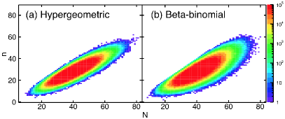
Figure 1: Correlation between $n$ and $N$ on the sample events, i.e. the magnitude of ${\cal R}(n;N)P(N)$, for the response matrices ${\cal R}_{\rm HG}(n;N)$ (hypergeometric) and ${\cal R}_{\beta}(n;N)$ (beta-binomial) with $p=X/Y=0.7$ and $Y=140$.

The procedure of the test analysis is as follows. We first generate sample events of $N$ by assuming the Poisson distribution for $P(N)$ with $\langle N\rangle=40$. We then specify the value of $n$ for each sample event randomly according to the probability ${\cal R}_{\rm HG}(n;N)$ or ${\cal R}_{\beta}(n;N)$. This allows one to obtain the moments $\mathopen{\hbox{${\langle}$}\mkern 2.0mu\kern-3.49998pt\leavevmode\hbox{${\langle}$}}n^{m}\mathclose{\hbox{${\rangle}$}\mkern 2.0mu\kern-3.49998pt\leavevmode\hbox{${\rangle}$}}$. These moments are used for the correction in Eq. (9). To proceed the correction, we take the following two different analyses. First, because the values of $r_{mj}$ are analytically known for ${\cal R}_{\rm HG}(n;N)$ and ${\cal R}_{\beta}(n;N)$, we perform the correction with these values. Besides this analysis, as a second option, we analyze $\langle N^{m}\rangle$ with the values of $r_{mj}$ determined by the fits to $R_{m}(N)$ obtained on the sample events with statistical errors. The second analysis supposes the correction of realistic detectors, of which the response matrix is obtained only stochastically.

In Fig. 1, we show the correlation between $n$ and $N$ on the $10^{8}$ sample events by plotting the two-dimensional histogram as a function of $n$ and $N$ for the hypergeometric (${\cal R}_{\rm HG}(n;N)$) and beta-binomial (${\cal R}_{\beta}(n;N)$) distributions with $p=0.7$ and $Y=140$. (This plot thus represents the magnitude of ${\cal R}(n;N)P(N)$, and is usually called the “response matrix” in literature for simplicity.) One finds from the figure that the distributions are clearly different between the two response matrices; the width of $n$ with fixed $N$ is narrower for ${\cal R}_{\rm HG}(n;N)$ than ${\cal R}_{\beta}(n;N)$.

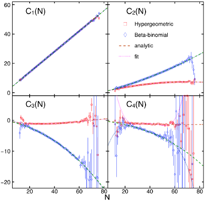
Figure 2: Cumulants of the response matrix $C_{m}(N)$ for ${\cal R}_{\rm HG}(n;N)$ and ${\cal R}_{\beta}(n;N)$ obtained on $10^{8}$ sample events with $p=0.7$ and $Y=140$. The dashed lines show the analytic values, while the dotted lines represent the fitting results with $m$th-order polynomial.

In Fig. 2, we show the cumulants of the response matrix $C_{m}(N)$ defined by

$$C_{1}(N)=R_{1}(N),\quad C_{2}(N)=R_{2}(N)-(R_{1}(N))^{2},$$ (20)

and so forth, for ${\cal R}_{\rm HG}(n;N)$ and ${\cal R}_{\beta}(n;N)$ obtained on $10^{8}$ sample events with $p=0.7$ and $Y=140$ for $m\leq 4$. The dashed lines show the analytic values, while the dotted lines are the fitting results with the $m$th-order polynomial. From these fits one obtains the values of $r_{mj}$.

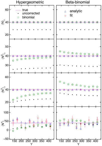
Figure 3: Cumulants obtained by the detector-response correction, $\langle N^{m}\rangle$, up to the fourth order with $p=0.7$ as functions of $Y$ for ${\cal R}_{\rm HG}(n;N)$ (left) and ${\cal R}_{\beta}(n;N)$ (right). The results obtained with the analytic (fitted) values of $r_{mj}$ are shown by triangles (squares). The corrected values agree with the true cumulants $\langle N^{m}\rangle_{\rm c}=40$ shown by the dashed line within statistics. The uncorrected cumulants $\mathopen{\hbox{${\langle}$}\mkern 2.0mu\kern-3.49998pt\leavevmode\hbox{${\langle}$}}n^{m}\mathclose{\hbox{${\rangle}$}\mkern 2.0mu\kern-3.49998pt\leavevmode\hbox{${\rangle}$}}_{\rm c}$ and the corrected results in the binomial model are also shown by circles and stars, respectively.

In Fig. 3, we show the corrected values of the cumulants $\langle N^{m}\rangle_{\rm c}$ for $m\leq 4$ with $p=0.7$ and various values of $Y$. The left (right) panel shows the results for ${\cal R}_{\rm HG}(n;N)$ (${\cal R}_{\beta}(n;N)$). The triangles represent the results obtained with the analytic values of $r_{mj}$, while the results obtained with $r_{mj}$ determined by the fits to $R_{m}(N)$ are shown by squares. $10^{7}$ sample events are used to obtain $\mathopen{\hbox{${\langle}$}\mkern 2.0mu\kern-3.49998pt\leavevmode\hbox{${\langle}$}}n^{m}\mathclose{\hbox{${\rangle}$}\mkern 2.0mu\kern-3.49998pt\leavevmode\hbox{${\rangle}$}}$ in both analyses, while $r_{mj}$ in the latter analysis are obtained with $10^{8}$ sample events. Errors are estimated by repeating the same simulation $100$ times. One finds from the figure that the corrected cumulants $\langle N^{m}\rangle_{\rm c}$ are consistent with the true value, $\langle N^{m}\rangle_{\rm c}=40$ shown by the dashed line, within statistics for all values of $Y$ in both analyses. In Fig. 3, the uncorrected cumulants, $\mathopen{\hbox{${\langle}$}\mkern 2.0mu\kern-3.49998pt\leavevmode\hbox{${\langle}$}}n^{m}\mathclose{\hbox{${\rangle}$}\mkern 2.0mu\kern-3.49998pt\leavevmode\hbox{${\rangle}$}}_{\rm c}$, are shown by filled circles. We also show the results of the efficiency correction with the binomial model with $p=0.7$ by the stars. The results in the binomial model fail in reproducing the true cumulants Bzdak et al. (2016), in contrast to the new method.

From Fig. 3 one also finds that the statistical error is large when $r_{mj}$ are determined by the fits, although the statistics to determine $r_{mj}$ is one order larger than that for $\mathopen{\hbox{${\langle}$}\mkern 2.0mu\kern-3.49998pt\leavevmode\hbox{${\langle}$}}n^{m}\mathclose{\hbox{${\rangle}$}\mkern 2.0mu\kern-3.49998pt\leavevmode\hbox{${\rangle}$}}$. This suggests that the suppression of the uncertainty of $r_{mj}$ is crucial in reducing the error of the final results.

Finally, we note that the fitting results of $C_{m}(N)$ in Fig. 2 have significant deviations from the analytic values for $N\gtrsim 60$. Nevertheless, the final results obtained with these fits reproduce the true values within statistics. This result shows that the detector-response correction is carried out appropriately even if the fits do not reproduce $R_{m}(N)$ in the range of $N$ at which $P(N)$ is small.

V Test analysis 2: Multiplicity-dependent efficiency

Next, we perform a test analysis of the detector-response correction for the response matrix which cannot be solved exactly. As such an example, we consider the response of a detector having a multiplicity-dependent efficiency. We consider the binomial distribution but the efficiency is dependent on $N$, i.e.

$${\cal R}_{\rm MD}(n;N)=B(n;p(N),N).$$ (21)

In typical detectors, the efficiency decreases with increasing multiplicity ($N$) Adamczyk et al. (2017); Holzmann . To model this behavior we assume

$$p(N)=0.7-\varepsilon(N-\langle N\rangle),$$ (22)

with $\varepsilon>0$

One can analytically show that the $m$th-order moment $R_{m}(N)$ of ${\cal R}_{\rm MD}(n;N)$ with Eq. (22) is given by the $2m$th-order polynomial. Therefore, the detector-response correction in this case cannot be solved exactly by the procedure in Sec. II.4. In the following, we use the truncated formulas discussed in Sec. II.5 with $L=4$.

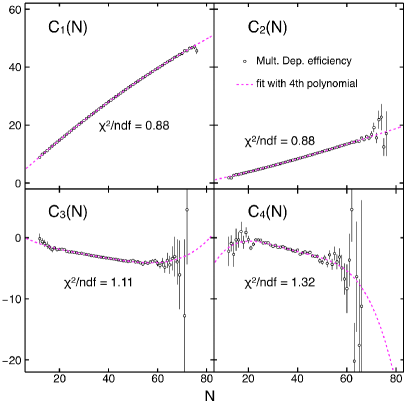
Figure 4: Cumulants $C_{m}(N)$ of the response matrix $R_{\rm MD}(n;N)$ with $p=0.7$ and $\varepsilon=0.002$ up to the fourth order obtained on $10^{8}$ sample events. The dashed lines show the results of the fits by the fourth order polynomial.

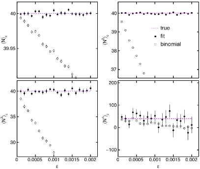
Figure 5: Filled circles show the corrected cumulants $\langle N^{m}\rangle_{\rm c}$ obtained by the truncation analysis for $R_{\rm MD}(n;N)$ as functions of $\varepsilon$. The corrected cumulants reproduce the true value $\langle N^{m}\rangle_{\rm c}=40$ for all $\varepsilon$ within statistics. The open circles show the corrected results in the binomial model.

For the test analysis, we generate the sample events of $N$ assuming the Poisson distribution with $\langle N\rangle=40$ for $P(N)$. The value of $n$ in each sample event is then specified according to ${\cal R}_{\rm MD}(n;N)$. $10^{8}$ sample events are generated in this way. Figure 4 shows the cumulants of the response matrix, $C_{m}(N)$, for $m\leq 4$ obtained from these sample events with $p=0.7$ and $\varepsilon=0.002$. We perform the fits to $R_{m}(N)$ with the fourth-order polynomial Eq. (16). The results of the fits in terms of $C_{m}(N)$ are shown by the dashed lines in Fig. 4. As shown in the figure, we have $\chi^{2}/{\rm ndf}\simeq 1$ for these fits, which suggests that the fits work well.

The results of the corrected cumulants, $\langle N^{m}\rangle_{\rm c}$, are shown in Fig. 5 by filled circles as a function of $\varepsilon$ for $m\leq 4$. Errors are estimated by the same procedure as in the previous section. The figure shows that the corrected results reproduce $\langle N^{m}\rangle_{\rm c}=40$ shown by the dashed line in each panel within statistics for all values of $\varepsilon$. In Fig. 5, we also show the cumulants obtained by the efficiency correction in the binomial model by the open circles. These results fail in reproducing the true cumulants even at $m=1$. Although the results in the binomial model are consistent with the true value for $m=4$, this agreement would be accidental. We note that the typical value of $\varepsilon$ for protons at the STAR detector is $\varepsilon\simeq 0.0002$ at $\sqrt{s_{\rm NN}}=7.7~{}$GeV, and $\varepsilon\simeq 0.0003$ at $\sqrt{s_{\rm NN}}=200~{}$GeV in Au+Au collisions    Nonaka . The maximal value of $\varepsilon$ in Fig. 5 is about one order larger than this value.

As discussed in Sec. III, in realistic experimental analysis we do not know the true distribution $P(N)$. This means that the distribution $P_{\rm MC}(N)$ used in the Monte Carlo simulation to determine ${\cal R}(n;N)$ is in general different from $P(N)$. In order to test the detector-response correction in such a case, we performed one more test analysis as follows: We use the Poisson distribution with $\langle N\rangle=40$ for $P(N)$ to determine $\mathopen{\hbox{${\langle}$}\mkern 2.0mu\kern-3.49998pt\leavevmode\hbox{${\langle}$}}n^{m}\mathclose{\hbox{${\rangle}$}\mkern 2.0mu\kern-3.49998pt\leavevmode\hbox{${\rangle}$}}$ as in the above analysis, but the values of $r_{mj}$ are determined by the fits to $R_{m}(N)$ generated by the Gauss distribution for $P_{\rm MC}(N)$ with $\langle N\rangle=\langle N^{2}\rangle_{\rm c}=40$. We checked that the final results in this analysis agrees with those shown in Fig. 5 within statistics even in this case. This result suggests that the detector-response correction with the strategy in Sec. III is applicable to realistic analyses.

VI Summary

In this paper, we proposed a new procedure to carry out the detector-response correction (including efficiency correction) of the higher order cumulants in the event-by-event analysis. This method provides exact formulas for various non-binomial response matrices, including Eqs. (18) and (19) parametrized by the hypergeometric and beta-binomial distributions. Introducing an approximation with the truncation, this method can deal with the correction of realistic detectors. The correction in this method is demonstrated explicitly for three non-binomial response matrices. We showed that the true cumulants are obtained within statistics not only for the exactly-solvable cases but also a case that the approximation with the truncation is necessary. Although we concentrated on the correction for the single-variable distribution throughout this manuscript, the extension to deal with the multi-variable distribution is also possible as discussed in Appendix A.” “

We thank M. Gazdzicki, R. Holzmann, A. Rustamov, M. Szala, and N. Xu for constructive discussions. M. K. thanks K. Redlich and B. Friman for inviting him to the workshop “Constraining the QCD Phase Boundary with Data from Heavy Ion Collisions” (Feb. 12-14, 2018, Darmstadt, Germany) and fruitful discussions during the workshop.

Appendix A Detector-response correction for multi-variable distribution

In this appendix, we discuss the extension of the detector-response correction to multi-variable distribution functions. This extension is necessary for the analysis of the net-particle number cumulants, because the net number is given by the difference of particle and anti-particle numbers. Also, the effects of the momentum and azimuthal angle dependence of the detector’s response can be described by the multi-variable distribution Nonaka et al. (2017).

For a simple illustration, we consider a distribution function of two particle species, $P(N_{1},N_{2})$, where $N_{1}$ and $N_{2}$ are the numbers of the particles in each event. We then denote the numbers of observed particles in each event as $n_{1}$ and $n_{2}$, respectively, and its event-by-event distribution as $\tilde{P}(n_{1},n_{2})$.

Similar to Eq. (1), we assume that these distribution functions are related with each other as

$$\tilde{P}(n_{1},n_{2})=\sum_{N_{1},N_{2}}{\cal R}(n_{1},n_{2};N_{1},N_{2})P(N_{1},N_{2}),$$ (23)

where the response matrix ${\cal R}(n_{1},n_{2};N_{1},N_{2})$ satisfies the normalization condition $\sum_{n_{1},n_{2}}{\cal R}(n_{1},n_{2};N_{1},N_{2})=1$.

Next, similar to Eq. (5) we consider the moments of ${\cal R}(n_{1},n_{2};N_{1},N_{2})$. In this case, because ${\cal R}(n_{1},n_{2};N_{1},N_{2})$ has two variables, we must consider the mixed moments,

$$R_{m_{1}m_{2}}(N_{1},N_{2})=\sum_{n_{1},n_{2}}n_{1}^{m_{1}}n_{2}^{m_{2}}{\cal R}(n_{1},n_{2};N_{1},N_{2}).$$ (24)

We then Taylor expand $R_{m_{1}m_{2}}(N_{1},N_{2})$,

$$R_{m_{1}m_{2}}(N_{1},N_{2})=\sum_{j_{1},j_{2}}r_{m_{1}m_{2};j_{1}j_{2}}N_{1}^{j_{1}}N_{2}^{j_{2}}.$$ (25)

Using Eq. (25), the mixed moments of observed particle numbers

$$\mathopen{\hbox{${\langle}$}\mkern 2.0mu\kern-3.49998pt\leavevmode\hbox{${\langle}$}}n_{1}^{m_{1}}n_{2}^{m_{2}}\mathclose{\hbox{${\rangle}$}\mkern 2.0mu\kern-3.49998pt\leavevmode\hbox{${\rangle}$}}=\sum_{n_{1},n_{2}}n_{1}^{m_{1}}n_{2}^{m_{2}}\tilde{P}(n_{1},n_{2})$$ (26)

are given by

$$\mathopen{\hbox{${\langle}$}\mkern 2.0mu\kern-3.49998pt\leavevmode\hbox{${\langle}$}}n_{1}^{m_{1}}n_{2}^{m_{2}}\mathclose{\hbox{${\rangle}$}\mkern 2.0mu\kern-3.49998pt\leavevmode\hbox{${\rangle}$}}=r_{m_{1}m_{2};00}+\sum_{j_{1},j_{2}}r_{m_{1}m_{2};j_{1}j_{2}}\langle N_{1}^{j_{1}}N_{2}^{j_{2}}\rangle.$$ (27)

We note that Eqs. (25) and (26) corresponds to Eqs. (6) and (7), respectively. In the matrix form, Eq. (27) is expressed as

$$\left[\begin{matrix}\mathopen{\hbox{${\langle}$}\mkern 2.0mu\kern-3.49998pt\leavevmode\hbox{${\langle}$}}n_{1}\mathclose{\hbox{${\rangle}$}\mkern 2.0mu\kern-3.49998pt\leavevmode\hbox{${\rangle}$}}\\ \mathopen{\hbox{${\langle}$}\mkern 2.0mu\kern-3.49998pt\leavevmode\hbox{${\langle}$}}n_{2}\mathclose{\hbox{${\rangle}$}\mkern 2.0mu\kern-3.49998pt\leavevmode\hbox{${\rangle}$}}\\ \mathopen{\hbox{${\langle}$}\mkern 2.0mu\kern-3.49998pt\leavevmode\hbox{${\langle}$}}n_{1}^{2}\mathclose{\hbox{${\rangle}$}\mkern 2.0mu\kern-3.49998pt\leavevmode\hbox{${\rangle}$}}\\ \mathopen{\hbox{${\langle}$}\mkern 2.0mu\kern-3.49998pt\leavevmode\hbox{${\langle}$}}n_{1}n_{2}\mathclose{\hbox{${\rangle}$}\mkern 2.0mu\kern-3.49998pt\leavevmode\hbox{${\rangle}$}}\\ \mathopen{\hbox{${\langle}$}\mkern 2.0mu\kern-3.49998pt\leavevmode\hbox{${\langle}$}}n_{2}^{2}\mathclose{\hbox{${\rangle}$}\mkern 2.0mu\kern-3.49998pt\leavevmode\hbox{${\rangle}$}}\\ \vdots\end{matrix}\right]=\left[\begin{matrix}r_{10;00}\\ r_{01;00}\\ r_{20;00}\\ r_{11;00}\\ r_{02;00}\\ \vdots\end{matrix}\right]+\bm{R}_{\rm mult}\left[\begin{matrix}\langle N_{1}\rangle\\ \langle N_{2}\rangle\\ \langle N_{1}^{2}\rangle\\ \langle N_{1}N_{2}\rangle\\ \langle N_{2}^{2}\rangle\\ \vdots\end{matrix}\right],$$ (28)

where the matrix $\bm{R}_{\rm mult}$ is composed of $r_{m_{1}m_{2};j_{1}j_{2}}$. By inversely solving Eq. (28) as in Eq. (9), one obtains the formulas to obtain the (mixed-)moments of the true distribution function $\langle N_{1}^{m_{1}}N_{2}^{m_{2}}\rangle$. The cumulants are then constructed from these moments; see Refs. Nonaka et al. (2017); Kitazawa and Luo (2017); De Wolf et al. (1996); Broniowski and Olszewski (2017), for the construction of the cumulants with multi-particle species. When the expansion Eq. (25) is not closed, one may truncate the expansion as in Eq. (16); the truncation at $j_{1}+j_{2}\leq L$ allows one to carry out the correction up to $L$th order.

This procedure can be generalized to the case with more than two-particle species in a straightforward manner.

Appendix B Alternative expansions of $R_{m}(N)$

In this appendix, we consider modification of the procedure in Sec. II with the use of alternative expansions of $R_{m}(N)$. These procedures give the same final result in principle, but might be effective in suppressing the accumulation of numerical errors in practical analyses.

First, instead of Eq. (16) we consider the Taylor expansion

$$R_{m}(N)=\sum_{j=0}^{L}\bar{r}_{mj}(N-N_{0})^{j}$$ (29)

at $N=N_{0}$ with an arbitrary number $N_{0}$. Substituting Eq. (29) into Eq. (4), one obtains

$$\left[\begin{matrix}\mathopen{\hbox{${\langle}$}\mkern 2.0mu\kern-3.49998pt\leavevmode\hbox{${\langle}$}}n\mathclose{\hbox{${\rangle}$}\mkern 2.0mu\kern-3.49998pt\leavevmode\hbox{${\rangle}$}}\\ \mathopen{\hbox{${\langle}$}\mkern 2.0mu\kern-3.49998pt\leavevmode\hbox{${\langle}$}}n^{2}\mathclose{\hbox{${\rangle}$}\mkern 2.0mu\kern-3.49998pt\leavevmode\hbox{${\rangle}$}}\\ \vdots\\ \mathopen{\hbox{${\langle}$}\mkern 2.0mu\kern-3.49998pt\leavevmode\hbox{${\langle}$}}n^{L}\mathclose{\hbox{${\rangle}$}\mkern 2.0mu\kern-3.49998pt\leavevmode\hbox{${\rangle}$}}\end{matrix}\right]=\left[\begin{matrix}\bar{r}_{10}\\ \bar{r}_{20}\\ \vdots\\ \bar{r}_{L0}\end{matrix}\right]+\bar{\bm{R}}\left[\begin{matrix}\langle N-N_{0}\rangle\\ \langle(N-N_{0})^{2}\rangle\\ \vdots\\ \langle(N-N_{0})^{L}\rangle\end{matrix}\right],$$ (30)

with $\bar{\bm{R}}=(\bar{r}_{mj})$. By choosing $N_{0}=\langle N\rangle$, Eq. (30) allows one to obtain the central moments $\langle(N-\langle N\rangle)^{m}\rangle$ directly.

We stress that Eq. (29) represents the same function as Eq. (16) with an appropriate replacement between $r_{mj}$ and $\bar{r}_{mj}$. Therefore, if these parameters are determined accurately Eqs. (17) and (30) give the same final result. However, they can give different results within numerical precision in practice. The use of Eq. (30) would be advantageous in reducing the numerical error, as the central moments are more closely related to cumulants than the standard moments.

Second, it is also possible to use expansions motivated by the factorial moments. One may expand $R_{m}(N)$ as

$$R_{m}(N)= f_{m0}+f_{m1}N+f_{m2}N(N-1)+\cdots$$

$$+f_{mj}N(N-1)\cdots(N-j+1)+\cdots.$$ (31)

Substituting this expansion into Eq. (4), one obtains

$$\left[\begin{matrix}\mathopen{\hbox{${\langle}$}\mkern 2.0mu\kern-3.49998pt\leavevmode\hbox{${\langle}$}}n\mathclose{\hbox{${\rangle}$}\mkern 2.0mu\kern-3.49998pt\leavevmode\hbox{${\rangle}$}}\\ \mathopen{\hbox{${\langle}$}\mkern 2.0mu\kern-3.49998pt\leavevmode\hbox{${\langle}$}}n^{2}\mathclose{\hbox{${\rangle}$}\mkern 2.0mu\kern-3.49998pt\leavevmode\hbox{${\rangle}$}}\\ \vdots\end{matrix}\right]=\left[\begin{matrix}f_{10}\\ f_{20}\\ \vdots\end{matrix}\right]+\bm{F}\left[\begin{matrix}\langle N\rangle_{\rm f}\\ \langle N^{2}\rangle_{\rm f}\\ \vdots\end{matrix}\right],$$ (32)

where $\bm{F}=(f_{mj})$ and

$$\langle N^{j}\rangle_{\rm f} =\langle N(N-1)\cdots(N-j+1)\rangle,$$ (33)

are the factorial moments of $P(n)$. Equation (32) provides formulas to obtain factorial moments $\langle N^{m}\rangle_{\rm f}$ directly.

One can also expand the factorial moments of ${\cal R}(n;N)$ as

$$R_{{\rm f},m}(N)= \sum_{n}n(n-1)\cdots(n-m+1){\cal R}(n;N)$$

$$= \bar{f}_{m0}+\bar{f}_{m1}N+\bar{f}_{m2}N(N-1)+\cdots$$

$$+\bar{f}_{m2}N(N-1)\cdots(N-j+1)+\cdots,$$ (34)

which enables us to connect $\langle N^{m}\rangle_{\rm f}$ with the factorial moments of $\tilde{P}(N)$, $\mathopen{\hbox{${\langle}$}\mkern 2.0mu\kern-3.49998pt\leavevmode\hbox{${\langle}$}}n^{m}\mathclose{\hbox{${\rangle}$}\mkern 2.0mu\kern-3.49998pt\leavevmode\hbox{${\rangle}$}}_{\rm f}$, directly as

$$\left[\begin{matrix}\mathopen{\hbox{${\langle}$}\mkern 2.0mu\kern-3.49998pt\leavevmode\hbox{${\langle}$}}n\mathclose{\hbox{${\rangle}$}\mkern 2.0mu\kern-3.49998pt\leavevmode\hbox{${\rangle}$}}_{\rm f}\\ \mathopen{\hbox{${\langle}$}\mkern 2.0mu\kern-3.49998pt\leavevmode\hbox{${\langle}$}}n^{2}\mathclose{\hbox{${\rangle}$}\mkern 2.0mu\kern-3.49998pt\leavevmode\hbox{${\rangle}$}}_{\rm f}\\ \vdots\end{matrix}\right]=\left[\begin{matrix}\bar{f}_{10}\\ \bar{f}_{20}\\ \vdots\end{matrix}\right]+\bar{\bm{F}}\left[\begin{matrix}\langle N\rangle_{\rm f}\\ \langle N^{2}\rangle_{\rm f}\\ \vdots\end{matrix}\right],$$ (35)

with $\bar{\bm{F}}=(\bar{f}_{mj})$. In the binomial model, $\bar{\bm{F}}$ is given by a diagonal matrix Kitazawa and Luo (2017). When ${\cal R}(n;N)$ is well approximated by the binomial model, therefore, the numerical analysis of the inverse matrix of $\bar{\bm{F}}$ would be more stable than that of $\bar{\bm{R}}$ .

Appendix C Binomial distribution with fluctuating probability

In this appendix, we calculate the moments of the binomial distribution Eq. (12) but the probability $p$ is fluctuating, i.e. the probability distribution given by

$$P_{N}(n)=\int_{0}^{1}dpG(p)B(n;p,N),$$ (36)

where $G(p)$ satisfies $\int_{0}^{1}dpG(p)=1$.

To obtain the moments of $P_{N}(n)$,

$$\langle n^{m}\rangle=\sum_{n}n^{m}P_{N}(n),$$ (37)

it is convenient to first calculate their factorial moments, which are given by

$$\langle n^{m}\rangle_{\rm f}=\sum_{n}n(n-1)\cdots(n-m+1)P_{N}(n)$$

$$=\int_{0}^{1}dpG(p)\sum_{n}n(n-1)\cdots(n-m+1)B(n;p,N)$$

$$=\int_{0}^{1}dpG(p)N(N-1)\cdots(N-m+1)p^{m}$$

$$=N(N-1)\cdots(N-m+1)\langle p^{m}\rangle_{\rm G},$$ (38)

where $\langle p^{m}\rangle_{\rm G}=\int_{0}^{1}dpp^{m}G(p)$ is the moments of $G(p)$ and in the last equality we used the relation

$$\sum_{n}n(n-1)\cdots(n-m+1)B(n;p,N)$$

$$=N(N-1)\cdots(N-m+1)p^{m}.$$ (39)

The moments of $P_{N}(n)$ is then obtained by converting Eq. (38) Kitazawa and Luo (2017). Explicit results up to the fourth order are

$$\langle n\rangle= \langle n\rangle_{\rm f}=\langle p\rangle_{\rm G}N,$$ (40)

$$\langle n^{2}\rangle= \langle n\rangle_{\rm f}+\langle n^{2}\rangle_{\rm f}=\langle p-p^{2}\rangle_{\rm G}N+\langle p^{2}\rangle_{\rm G}N^{2},$$ (41)

$$\langle n^{3}\rangle= \langle n\rangle_{\rm f}+3\langle n^{2}\rangle_{\rm f}+\langle n^{3}\rangle_{\rm f}$$

$$= \langle p-3p^{2}+2p^{3}\rangle_{\rm G}N+3\langle p^{2}-p^{3}\rangle_{\rm G}N^{2}+\langle p^{3}\rangle_{\rm G}N^{3},$$ (42)

$$\langle n^{4}\rangle= \langle n\rangle_{\rm f}+7\langle n^{2}\rangle_{\rm f}+6\langle n^{3}\rangle_{\rm f}+\langle n^{4}\rangle_{\rm f}$$

$$= \langle p-7p^{2}+12p^{3}-6p^{4}\rangle_{\rm G}N$$

$$+\langle 7p^{2}-18p^{3}+11p^{4}\rangle_{\rm G}N^{2}$$

$$+6\langle p^{3}-p^{4}\rangle_{\rm G}N^{3}+\langle p^{4}\rangle_{\rm G}N^{4}.$$ (43)

The same manipulation can be repeated for arbitrary higher orders. From this derivation, it is clear that the $m$th-order moments of $P_{N}(n)$ are given by the $m$th-order polynomial of $N$.

Appendix D Hypergeometric and beta-binomial distributions

In this appendix we summarize the definitions and properties of the hypergeometric and beta-binomial distributions.

We define the hypergeometric and beta-binomial distributions, $H(n;N,X,Y)$ and $\beta(n;N,a,b)$, as

$$H(n;N,X,Y)$$

$$=\frac{X!}{n!(X-n)!}\frac{(Y-X)!}{(N-n)!(X-n)!}\frac{N!(Y-N)!}{Y!},$$ (44)

and

$$\beta(n;N,a,b)=\int_{0}^{1}dp{\cal B}(p;a,b)B(n;p,N),$$ (45)

with the beta distribution

$${\cal B}(p;a,b)=p^{a}(1-p)^{b}/B(a,b),$$ (46)

where $B(a,b)$ is the beta function required for the normalization $\int_{0}^{1}dp{\cal B}(p;a,b)=1$.

The hypergeometric and beta distributions are given in urn models as follows. First, we consider $N_{\rm w}$ white balls and $N_{\rm b}$ black balls in an urn, and draw $N$ balls from the urn without returning balls to the urn in each draw. Then, the probability distribution of the number of white balls, $n$, is given by the hypergeometric distribution as $H(n;N,N_{\rm w},N_{\rm tot})$ with $N_{\rm tot}=N_{\rm w}+N_{\rm b}$. Next, we consider successive draws of the balls from the urn. In each draw, when one draws a white (black) ball, two white (black) balls are returned to the urn. After repeating this procedure $N$ times, the probability distribution to draw $n$ white balls in total is given by the beta-binomial distribution as $\beta(n;N,N_{\rm w},N_{\rm b})$. The distributions of $n$ in both urn models become close to the binomial distribution $B(n;p,N)$ in the limit $N_{\rm tot}\to\infty$ with fixed $p=N_{\rm w}/N_{\rm tot}$, where $p$ represents the probability to draw a white ball in a draw. This means that $H(n;N,X,Y)$ and $\beta(n;N,a,b)$ approach the binomial distribution in the limit $Y\to\infty$ with fixed $X/Y$ and $a\to\infty$ with fixed $a/(a+b)$, respectively.

The cumulants of Eqs. (44) and (45), $\langle n^{m}\rangle_{\rm c}^{\rm HG}$ and $\langle n^{m}\rangle_{\rm c}^{\beta}$, respectively, up to the fourth order are given by

$$\langle n\rangle_{\rm c}^{\rm HG} = Np,$$ (47)

$$\langle n^{2}\rangle_{\rm c}^{\rm HG} = \frac{N(N-Y)(-1+p)p}{-1+Y},$$ (48)

$$\langle n^{3}\rangle_{\rm c}^{\rm HG} = \frac{N(2N^{2}-3NY+Y^{2})(-1+p)p(-1+2p)}{(-2+Y)(-1+Y)},$$ (49)

$$\langle n^{4}\rangle_{\rm c}^{\rm HG} = [N(N-Y)(-1+p)p(6N^{2}(-1-6(-1+p)p+Y(1+5(-1+p)p))$$ (50)

$$-6NY(-1-6(-1+p)p+Y(1+5(-1+p)p))$$

$$+(-1+Y)Y(1+Y(1+6(-1+p)p)))]/\left[(-3+Y)(-2+Y)(-1+Y)^{2}\right],$$

$$\langle n\rangle_{\rm c}^{\beta} = Np,$$ (51)

$$\langle n\rangle_{\rm c}^{\beta} = -\frac{N(N+a+b)(-1+p)p}{1+a+b},$$ (52)

$$\langle n\rangle_{\rm c}^{\beta} = \frac{N(N+a+b)(2N+a+b)(-1+p)p(-1+2p)}{(1+a+b)(2+a+b)},$$ (53)

$$\langle n\rangle_{\rm c}^{\beta} = -((N(N+a+b)(-1+p)p(6N^{2}(1+6(-1+p)p+(a+b)(1+5(-1+p)p))$$ (54)

$$+6N(a+b)(1+6(-1+p)p+(a+b)(1+5(-1+p)p))+(a+b)(1+a+b)$$

$$(-1+(a+b)(1+6(-1+p)p))))/((1+a+b)^{2}(2+a+b)(3+a+b))).$$

As one finds from Eq. (48) (Eq. (52)), the hypergeometric (beta-binomial) distribution is narrower (wider) than the binomial distribution with $\langle n^{2}\rangle_{\rm c}=p(1-p)N$.

As the $m$th-order cumulants are given by the $m$th-order polynomial in Eqs. (47)–(54), the $m$th-order moments of Eqs. (44) and (45) are also given by $m$th-order polynomial. The values of $r_{mj}$ are obtained as the coefficients of the moments.

References

- Asakawa and Kitazawa (2016) M. Asakawa and M. Kitazawa, Prog. Part. Nucl. Phys. 90, 299 (2016), arXiv:1512.05038 [nucl-th] .
- Luo and Xu (2017) X. Luo and N. Xu, Nucl. Sci. Tech. 28, 112 (2017), arXiv:1701.02105 [nucl-ex] .
- Ejiri et al. (2006) S. Ejiri, F. Karsch, and K. Redlich, Phys. Lett. B633, 275 (2006), arXiv:hep-ph/0509051 [hep-ph] .
- Stephanov (2009) M. A. Stephanov, Phys. Rev. Lett. 102, 032301 (2009), arXiv:0809.3450 [hep-ph] .
- Asakawa et al. (2009) M. Asakawa, S. Ejiri, and M. Kitazawa, Phys. Rev. Lett. 103, 262301 (2009), arXiv:0904.2089 [nucl-th] .
- Adamczyk et al. (2014a) L. Adamczyk et al. (STAR), Phys. Rev. Lett. 112, 032302 (2014a), arXiv:1309.5681 [nucl-ex] .
- Adamczyk et al. (2014b) L. Adamczyk et al. (STAR), Phys. Rev. Lett. 113, 092301 (2014b), arXiv:1402.1558 [nucl-ex] .
- Adare et al. (2016) A. Adare et al. (PHENIX), Phys. Rev. C93, 011901 (2016), arXiv:1506.07834 [nucl-ex] .
- Adamczyk et al. (2017) L. Adamczyk et al. (STAR), (2017), arXiv:1709.00773 [nucl-ex] .
- Abelev et al. (2013) B. Abelev et al. (ALICE), Phys. Rev. Lett. 110, 152301 (2013), arXiv:1207.6068 [nucl-ex] .
- Rustamov (2017) A. Rustamov (ALICE), Proceedings, 26th International Conference on Ultra-relativistic Nucleus-Nucleus Collisions (Quark Matter 2017): Chicago, Illinois, USA, February 5-11, 2017, Nucl. Phys. A967, 453 (2017), arXiv:1704.05329 [nucl-ex] .
- (12) M. Gazdzicki, talk at “Constraining the QCD Phase Boundary with Data from Heavy Ion Collisions” (Darmstadt, Germany, Feb. 12-14, 2018).
- (13) R. Holzmann (HADES), Talk at “26th International Conference on Ultra-relativistic Nucleus-Nucleus Collisions (Quark Matter 2017)” (Chicago, Illinois, USA, Feb. 5-11, 2017).
- (14) H. Sako et al., “White paper for a Future J-PARC Heavy-Ion Program (J-PARC-HI),” http://asrc.jaea.go.jp/soshiki/gr/hadron/jparc-hi/.
- Rapp et al. (2011) R. Rapp et al., Lect. Notes Phys. 814, 335 (2011).
- Blaschke et al. (2016) D. Blaschke et al., Eur. Phys. J. A 52, 299 (2016).
- Kitazawa and Asakawa (2012) M. Kitazawa and M. Asakawa, Phys. Rev. C86, 024904 (2012), [Erratum: Phys. Rev.C86,069902(2012)], arXiv:1205.3292 [nucl-th] .
- Bialas and Peschanski (1986) A. Bialas and R. B. Peschanski, Nucl. Phys. B273, 703 (1986).
- Bzdak and Koch (2012) A. Bzdak and V. Koch, Phys. Rev. C86, 044904 (2012), arXiv:1206.4286 [nucl-th] .
- Bzdak and Koch (2015) A. Bzdak and V. Koch, Phys. Rev. C91, 027901 (2015), arXiv:1312.4574 [nucl-th] .
- Luo (2015a) X. Luo, Phys. Rev. C91, 034907 (2015a), arXiv:1410.3914 [physics.data-an] .
- Kitazawa (2016) M. Kitazawa, Phys. Rev. C93, 044911 (2016), arXiv:1602.01234 [nucl-th] .
- Nonaka et al. (2016) T. Nonaka, T. Sugiura, S. Esumi, H. Masui, and X. Luo, Phys. Rev. C94, 034909 (2016), arXiv:1604.06212 [nucl-th] .
- Nonaka et al. (2017) T. Nonaka, M. Kitazawa, and S. Esumi, Phys. Rev. C95, 064912 (2017), arXiv:1702.07106 [physics.data-an] .
- Esha (2017) R. Esha (STAR), Proceedings, 26th International Conference on Ultra-relativistic Nucleus-Nucleus Collisions (Quark Matter 2017): Chicago, Illinois, USA, February 5-11, 2017, Nucl. Phys. A967, 457 (2017).
- Luo (2015b) X. Luo (STAR), Proceedings, 9th International Workshop on Critical Point and Onset of Deconfinement (CPOD 2014): Bielefeld, Germany, November 17-21, 2014, PoS CPOD2014, 019 (2015b), arXiv:1503.02558 [nucl-ex] .
- Bzdak et al. (2016) A. Bzdak, R. Holzmann, and V. Koch, Phys. Rev. C94, 064907 (2016), arXiv:1603.09057 [nucl-th] .
- D’Agostini (1995) G. D’Agostini, Nucl. Instrum. Meth. A362, 487 (1995).
- Adye (2011) T. Adye, in Proceedings, PHYSTAT 2011 Workshop on Statistical Issues Related to Discovery Claims in Search Experiments and Unfolding, CERN,Geneva, Switzerland 17-20 January 2011, CERN (CERN, Geneva, 2011) pp. 313–318, arXiv:1105.1160 [physics.data-an] .
- Garg et al. (2013) P. Garg, D. K. Mishra, P. K. Netrakanti, A. K. Mohanty, and B. Mohanty, J. Phys. G40, 055103 (2013), arXiv:1211.2074 [nucl-ex] .
- He and Luo (2018) S. He and X. Luo, (2018), arXiv:1802.02911 [physics.data-an] .
- Agostinelli et al. (2003) S. Agostinelli et al. (GEANT4), Nucl. Instrum. Meth. A506, 250 (2003).
- (33) T. Nonaka, talk at “XII Workshop on Particle Correlations and Femtoscopy ” (Nikhef, Amsterdam, The Netherlands, Jun. 12-16, 2017).
- Kitazawa and Luo (2017) M. Kitazawa and X. Luo, Phys. Rev. C96, 024910 (2017), arXiv:1704.04909 [nucl-th] .
- De Wolf et al. (1996) E. A. De Wolf, I. M. Dremin, and W. Kittel, Phys. Rept. 270, 1 (1996), arXiv:hep-ph/9508325 [hep-ph] .
- Broniowski and Olszewski (2017) W. Broniowski and A. Olszewski, Phys. Rev. C95, 064910 (2017), arXiv:1704.01532 [nucl-th] .