The central velocity dispersion of the Milky Way bulge

Abstract

Context. Recent spectroscopic and photometric surveys are providing a comprehensive view of the Milky Way bulge stellar population properties with unprecedented accuracy. This in turn allows us to explore the correlation between kinematics and stellar density distribution, crucial to constraint the models of Galactic bulge formation.

Aims. The Giraffe Inner Bulge Survey (GIBS) revealed the presence of a velocity dispersion peak in the central few degrees of the Galaxy by consistently measuring high velocity dispersion in three central most fields. Due to suboptimal distribution of these fields, all being at negative latitudes and close to each other, the shape and extension of the sigma peak is poorly constrained. In this study we address this by adding new observations distributed more uniformly and in particular including fields at positive latitudes that were missing in GIBS.

Methods. MUSE observations were collected in four fields at $(l,b)=(0^{\circ},+2^{\circ}),(0^{\circ},-2^{\circ})$, $(+1^{\circ},-1^{\circ})$, and $(-1^{\circ},+2^{\circ})$. Individual stellar spectra were extracted for a number of stars comprised between $\sim$500 and $\sim$1200, depending on the seeing and the exposure time. Velocity measurements are done by cross-correlating observed stellar spectra in the CaT region with a synthetic template, and velocity errors obtained through Monte Carlo simulations, cross-correlating synthetic spectra with a range of different metallicities and different noise characteristics.

Results. We measure the central velocity dispersion peak within a projected distance from the Galactic center of $\sim$280 pc, reaching $\sigma V_{GC}\sim$140 km/s at b=-1^∘. This is in agreement with the results obtained previously by GIBS at negative longitude. The central sigma peak is symmetric with respect to the Galactic plane, with a longitude extension at least as narrow as predicted by GIBS.

As a result of the Monte Carlo simulations we present analytical equations for the radial velocity measurement error as a function of metallicity and signal-to-noise ratio for giant and dwarf stars.

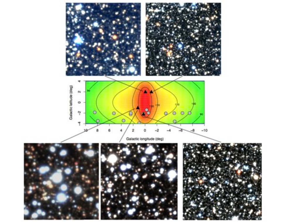
Figure 1: VRI MUSE FOV coloured images of the bulge $1^{\prime}\times 1^{\prime}$ fields analysed here, from top left clockwise: p0p2, m1p2, p0m2, and two pointings at p1m1 highlighting the impact of different image quality. Their Galactic position relative to the velocity dispersion map of Zoccali et al. (2014) is also shown.

1 Introduction

Recent photometric and spectroscopic surveys of the Galactic bulge are providing a wealth of data to explore the spatial distribution, chemical content and kinematics of its stellar population. A special 2016 edition of the Publications of the Astronomical Society of Australia (vol. 33) provides several reviews on the bulgenobservational properties (e.g., Zoccali & Valenti, 2016; Babusiaux, 2016).

Stellar kinematics and spatial distribution, in particular, are thought to be strongly correlated with the bulge formation process. Two main scenarios have been proposed for bulge formation. The first one through evolution of the disk, when the latter had been mostly converted into stars. In this case the bulge is expected to have the shape of a bar, though vertically heated into a boxy/peanut, with corresponding kinematics. The second one is the hierarchical merging of gas rich sub-clumps coming either from the disk or from satellite structures. In this case both the spatial distribution and the kinematics are expected to be more isotropic. Obviously, a combination of these two scenarios could have also led to the formation of the Galactic bulge we observed today.

Early kinematical surveys covering a large bulge area such as BRAVA (Rich et al., 2007; Howard et al., 2009) and ARGOS (Freeman et al., 2013; Ness et al., 2013a, b) derived a rotation curve that looked cylindrical, supporting the conclusion that the bulge had been formed exclusively via disk dynamical instabilities (Shen et al., 2010). These studies, however, were limited – by crowding and interstellar extinction – to latitudes $|b|>4^{\circ}$. By using data from the GIRAFFE Inner Bulge Survey (GIBS), Zoccali et al. (2014) found that the radial velocity dispersion ($\sigma$) exhibits a strong increase resulting in a peak with $\sim$140 km/s, confined within a radius of $\sim$250 pc from the Galactic center. It was later demostrated that this peak is spatially associated to a peak in star counts (Valenti et al., 2016), hence in stellar mass, and it is slightly dominated by metal poor stars (Zoccali et al., 2017).

Indeed, there is now consensus that the inner Galactic bulge hosts two components that are best separated in metallicity ([Fe/H]) , but also show different spatial distribution (Ness et al., 2012; Dékány et al., 2013; Rojas-Arriagada et al., 2014; Pietrukowicz et al., 2015; Gran et al., 2016; Zoccali et al., 2017), kinematics (Babusiaux et al., 2010; Zoccali et al., 2017) and [Mg/Fe] ratio (Hill et al., 2011).

The velocity dispersion peak found from GIBS data was constrained by three fields, at galactic coordinates ($l,b$) = ($-0.26^{\circ}$, $-1.40^{\circ}$) (0.27^∘, $-2.13^{\circ}$) and ($-0.58^{\circ}$, $-1.98^{\circ}$), respectively. The velocity dispersion was derived from samples of 441, 435 and 111 stars, respectively. The need to obtain intermediate resolution optical spectra for many stars, with a signal-to-noise ratio (SNR) high enough to allow us to measure Calcium II Triplet (CaT) metallicity, restricted the position of the GIBS innermost fields to the bulge hemisphere at negative latitudes. In order to constrain the shape and spatial extension of the $\sigma$-peak, we analyse here new data obtained with the MUSE IFU spectrograph at the ESO VLT, in fields closer to the Galactic center at both positive and negative latitudes.

2 Observations and data reduction

Three fields, hereafter named p0m2, p0p2 and m1p2, located in the innermost bulge regions were observed with MUSE during the Science Verification campaign. Another one, consisting of two adjacent pointings, named p1m1-A and p1m1-B, was observed in Service Mode as part of a filler program 99.B-0311A (PI: Valenti) for which only 4 hours were executed of the 76 hours originally approved. Table 1 lists the Galactic coordinates, exposure times, image quality and interstellar extinction (Gonzalez et al., 2012) for all the fields. The two pointings of the p1m1 field were observed under quite different seeing conditions, but they are so close to each other that they have the same velocity dispersion, and are thus treated as a single field hereafter.

MUSE (Bacon et al., 2010) is the integral field spectrograph at the Nasmyth B focus of the Yepun (VLT-UT4) telescope at ESO Paranal Observatory. It provides 1 square arcmin field of view, with a spatial pixel of 0.2”, and a mean spectral resolution of $R\approx 3000$. The observations were carried out in seeing limited mode (WFM-noAO) by using the so-called Nominal setup, which yields a continuous wavelength coverage between 4750$\AA$ and 9350$\AA$.

For all the fields, we used similar observing strategy but different total integration time (see Table 1): a combination of on-target sub-exposures each $\sim$1000 sec long, taken with a small offsets pattern (i.e. $\sim$1.5”) and $90^{\circ}$ rotations in order to optimise the cosmics rejection and obtaining a uniform combined dataset in terms of noise properties.

The processing of the raw data was performed with the MUSE pipeline (v.1.5, Weilbacher et al., 2012). The entire pipeline data reduction cascade consists of two main steps: i) creating all necessary calibrations to remove the instrument signature from each target exposures, such as bias, flats, bad pixels map, instrument geometry, illumination, astrometry correction, line spread function, response curve for flux calibration, and wavelength solution map; and ii) constructing, for each target field, the final datacube by combining the different science exposures processed during the previous step. In addition to the final datacube, the pipeline optionally produces the so-called Field-of-View (FoV) images by convolving the MUSE datacube with the transmission curve of various filters. For this work we produced FoV images in $V$-Johnson, $R$-Cousins and $I$-Cousins. Fig. 1 shows the color image of each target field obtained combining the $V$, $R$ and $I$ FoV images, and the position of the four fields in the velocity dispersion map provided by the GIBS survey. Clearly, the number of stars detected in each field is affected both by the different seeing conditions and by the extinction of the field.

Table 1: Galactic coordinates, reddening, image quality and observations Log of the observed fields.

Field	$l$	$b$	Exp. Time	FWHM	E($J-Ks$)
p0m2	+0.26∘	$-$2.14∘	6 $\times$ 1000 s	0.6”	0.36
m1p2	$-$1.00∘	+2.00∘	2 $\times$ 1000 s	0.5”	0.86
p0p2	0.00∘	+2.00∘	3 $\times$ 1000 s	1.1”	0.90
p1m1-A	+1.20∘	$-$1.00∘	6 $\times$ 1066 s	1.2”	0.87
p1m1-B	+1.20∘	$-$1.00∘	6 $\times$ 1066 s	0.9”	0.86

2.1 Extraction of the spectra

The procedure adopted to extract the spectra for all the stellar sources present in the target fields consists of two main steps: i) the creation of a master star list for each field; and ii) the reconstruction of the spectrum of each star in the list, by using the star flux as measured in the MUSE final data cubes.

We first performed standard aperture photometry, with DAOPHOT (Stetson, 1987), on the FoV images to obtain a master list of all sources with significant counts ($>4\sigma$) above the background. Due to the relatively modest crowding, aperture or PSF-fitting photometry yield virtually identical results, therefore we used aperture photometry hereafter (see below). Fig. 2 shows the derived color-magnitude diagrams (CMDs) for all the fields, either in the ($R$, $V-R$) or in the ($R$, $R-I$) instrumental plane. The latter was used for the p1m1 field because, due to its higher extinction, the $V$ image had the lowest SNR. Here the impact of the different seeing and total exposure time is also very clear, with the p0p2 field being the least populated, due to the combination of relatively poor seeing and short total exposure time. The p1m1 field is the closest one to the Galactic plane, therefore showing a prominent disk main sequence (MS) that is both more prominent and extends to brighter magnitudes in comparison to the other fields. This is due to the fact that at $b=-1^{\circ}$ the optical depth of the thin disk is larger. The presence of bright blue stars is very evident also in the FoV images of Fig. 1

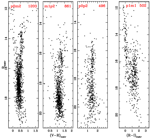
Figure 2: Instrumental CMD of the observed bulge fields as derived by running aperture photometry on the MUSE FoV images. The name of the fields and total number of detected stars are given.

The final MUSE data cubes were then sliced along the wavelength axis into 3681 monochromatic images (i.e. single planes) sampling the target stars from 4750$\AA$ to 9350$\AA$ with a step in wavelength of 1.25 $\AA$. Aperture photometry was performed on each of these images (task PHOT of IRAF) with an aperture radius $\sim$  1.5 $\times\,<FWHM>$, where $<FWHM>$ is the average image quality measured over the wavelength range $\lambda>$ 6000$\AA$. Finally, for each star in the master list, the corresponding spectrum was obtained by assigning to each wavelength the flux measured on the corresponding monochromatic image. For a given field, a single value was used for the aperture radius, since the FWHM variation, as measured across the entire wavelength range, is about half a pixel, independent from the mean FWHM value.

It is worth mentioning that this photometric approach to the extraction of IFU spectra has the advantage of successfully addressing the issue of sky subtraction residuals often present in the final data cubes. Indeed, it is well known that the sky subtraction may be not always optimal, leading to the presence of artefacts (e.g. weak emission line residuals and/or p cygni-like profiles) in the final spectra. By contrast, any such residuals present in the single plane images are fully taken into account by the photometric procedure, which estimates a local sky background for each source present in the master list.

Several attempts at using PSF-fitting photometry on the monochromatic images were performed. They were finally discarded because the majority of the stars were lost in a few of the monochromatic images, corresponding to the bottom of their strongest absorption lines. When the star flux is close to the sky level, aperture photometry still assigns a meaningful flux value, while PSF-fitting photometry just discards the star from the list. This is not a negligible issue, given that the strong absorption lines are very important in the measurement of radial velocities. On the other hand, given the modest crowding of the images, the photometry from aperture and PSF-fitting yielded similar quality result, at least on the FoV images. Therefore we judged not necessary, in this case, to try and overcome the problem of non-convergence of the PSF in the low signal regime. The analysis of more crowded fields such as the inner regions of dense star clusters might require some different approach.

Spectra for 1203, 861, 496 and 502 stars were reconstructed in the p0m2, m1p2, p0p2 and p1m1 fields, respectively. Examples of typical extracted spectra, zoomed in the CaT region, for stars of different magnitudes are given in Fig. 3. We show spectra for the field with the best combination of seeing and exposure time (p0m2) and the one with the worst seeing (p1m1-A). The average SNR, as measured in the CaT wavelength range, of field p0m2, m1p2, p0p2 and p1m1 stars in the faintest 0.5 mag bin is $\sim$ 20, 15, 10, 10 respectively.

Figure 3: Example of typical spectra in the CaT region, for stars in the brightest 0.5 mag bin, for red clump stars, and star at the very faint-end magnitude range. For each spectrum, the instrumental R magnitude of the star is given.

3 Radial velocities and velocity errors

We measured the heliocentric radial velocity (RV) of all stars detected in the observed fields through cross-correlation with a synthetic template by using the IRAF task fxcor. Specifically, we adopted for all stars the same synthetic spectra of a relatively metal rich ([Fe/H]$=-0.4$ dex) K giant and performed the cross-correlation between the model and the observed spectra in the wavelength range bracketing the CaT lines. To assess the effect that the use of a single metallicity template may have on the derived velocities, in the case of p0m2 stars field, we also used 2 additional synthetic templates with metallicities ([Fe/H]$=-1.3$ dex and $+0.2$ dex) that bracket the typical metallicity distribution function observed in the GIBS fields by Zoccali et al. (2017). We found that the RV derived with the metal-poor and metal-rich models always agree within $\leq\,1$ km/s, thus confirming what already noticed by Zoccali et al. (2014) that the metallicity of the adopted synthetic template has a very minor effect on the derived RV.

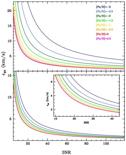
Figure 4: RV error ($\epsilon_{RV}$) profile as a function of the spectra SNR for giants (bottom panel) and dwarf (top panel) of different metallicity. The inset shows the $\epsilon_{RV}$ profile of giants in the medium-low SNR regime.

The error in the derived RV could not be estimated from repeated measurements because, for each target field , we only have one single data-cube. Therefore, the uncertainty ($\epsilon_{RV}$) has been estimated by means of MonteCarlo simulations. The main sources of uncertainties are the SNR, the spectral resolution, and the sampling. In order to evaluate their impact on the derived RVs we generated different sets of artificial MUSE spectra, varying SNR and metallicity, reproducing the observed ones. We started from synthetic spectra calculated with the code SYNTHE (Sbordone et al., 2004), assuming typical parameters of a giant ($T_{eff}$= 4500 K, log g=1.5, $v_{turb}$=2 km/s) and a dwarf star ($T_{eff}$= 6500 K, log g=4.5, $v_{turb}$=1 km/s), and considering a grid of metallicity between [Fe/H]=$-$3.0 and +0.5 dex with a step of 0.5 dex. These synthetic spectra have been convolved with a Gaussian profile to reproduce the spectral resolution of MUSE and then resampled at the same pixel size of the observed extracted spectra (1.25 Å/pixel). Poisson noise was added to the synthetic spectra in order to reproduce different noise conditions, from SNR$\sim$10 to SNR$\sim$100 with steps of 10. At the end, for each metallicity and SNR, a sample of 500 synthetic spectra with randomly added noise was generated and their RVs measured through cross-correlation technique (fxcor) with the original synthetic spectrum as template.

The dispersion of the derived RVs of each sample has been assumed as 1$\sigma$ uncertainty in the RV measurement for a given SNR and metallicity. We derived the following relations that link the radial velocity error to SNR and metallicity for giant stars (1):

$$$$\ln(\epsilon_{RV})=4.209-0.997\ln({\rm SNR})-0.029{\rm[Fe/H]}+0.058{\rm[Fe/H]}^{2}$$$$ (1)

and for dwarf stars (2):

$$$$\ln(\epsilon_{RV})=4.624-1.023\ln({\rm SNR})-0.159{\rm[Fe/H]}+0.120{\rm[Fe/H]}^{2}$$$$ (2)

The behaviour of $\epsilon_{RV}$ as a function of SNR for different values of [Fe/H] is shown in Fig. 4 for giant and dwarf stars. For giant stars $\epsilon_{RV}$ increases rapidly for SNR smaller than 30, reaching uncertainties at SNR= 10 of 6.8 and 12.5 km/s for [Fe/H]=+0.5 and –3.0 dex, respectively, while at high SNR $\epsilon_{RV}$ is almost constant and close $\sim$1 km/s. At a given SNR, $\epsilon_{RV}$ increases as decreasing [Fe/H], due to the weakening of the CaT lines, while for [Fe/H] larger than -1.0 dex the curves are almost indistinguishable. A similar general behaviour is found also for the dwarf stars, but with larger uncertainties because of the weakness of the CaT lines: in particular at SNR= 10, the relation provides $\epsilon_{RV}$= 9.2 km/s for [Fe/H]=+0.5 dex, while at lower metallicities the uncertainties increase dramatically (up to $\sim$45 km/s for [Fe/H]=–3.0 dex). Note that we limited this procedure to the CaT lines spectral region, in a window between 8450 Åand 8700 Å, hence these relations are specific to the case of MUSE in this spectral window.

For each field, Table 2 lists the errors on the RV estimates for stars in the faintest 0.5 mag bin as derived by using the above mentioned relations for two different metallicity values: [Fe/H]=–1 dex and [Fe/H]=+0.5 dex, which represent the metal-poor and metal-rich edge of the typical bulge metallicity distribution function. In particular, due to the differences in the magnitude depth among the different fields, the values quoted in Table 2 have been derived by using equation (2) for the p0m2, m1p2 and p0p2 fields, whereas for p1m1 we have adopted the relation for giants (i.e. equation (1)). As expected, we found that at fixed SNR (i.e. magnitude) metal-rich stars have typically smaller radial velocity error. However, the variation over the entire bulge metallicity range is $\leq\,2$ km/s (see Table2 and Fig.4).

Table 2: Typical radial velocity error of observed stars in the faintest 0.5 mag bin as derived from equation (2) for [Fe/H]=–1 dex (MP) and [Fe/H]=+0.5 dex (MR).

Field	SNR	$\epsilon_{RV}$ (MP)	$\epsilon_{RV}$ (MR)
		km/s	km/s
p0m2	20	6.3	4.5
m1p2	15	8.4	6.1
p0p2	10	12.8	9.2
p1m1a	10	7.4	6.8
(a)For this field the faintest stars are giants,
therefore we have used equation (1).

4 Velocity dispersion

In order to measure the velocity dispersion of bulge stars, it is important to take into account the contamination by foreground disk stars, which are known to have a smaller velocity dispersion (Ness et al., 2016; Robin et al., 2017). An estimate of the actual disk velocity dispersion can be attempted by selecting foreground disk MS stars in the instrumental CMD of each observed field. This is shown in Figs. 5-8. Thanks to the good seeing, longer exposure time and relatively low reddening, the p0m2 field has the best defined CMD, reaching fainter magnitudes (Fig. 5). In this field, bona fide bulge-RGB/disk-MS stars (red/blue symbols, respectively) are selected as having both $R<16$ and $(V-R)$ larger/smaller than $0.35$, respectively. The cuts isolate 75 disk MS stars, shown in blue in the CMD, and 206 bulge RGB stars shown in red. Stars fainter than $R=16$, plotted in green, cannot be safely assigned to either population. The top-right panels of Figs. 5-8 shows the heliocentric radial velocity versus magnitude, for all the stars, with the same color coding as before. It is clear that disk MS stars have a lower velocity dispersion, but, as expected, their radial velocity distribution is contaminated by bulge stars, both blue stragglers and sub giant branch stars. In fact, the radial velocity histogram shown at the bottom of the right panel clearly shows the presence of outliers at $|RV|>150$ km/s. Indeed, if these stars are excluded, by a simple cut at $|RV|<120$ km/s, the radial velocity dispersion drops to a value of $\sigma_{\rm RV}=45$ km/s, consistent in all three fields at $b=\pm 2^{\circ}$.

This exercise allows us to conclude that in the region of the CMDs above the old MS turnoff, where we can safely separate disk foreground from bulge stars by means of a color cut, the velocity dispersion of the disk is significantly lower than that of the bulge. Therefore, in order to include bulge MS stars in our analysis, we need to allow for the presence of two components with different kinematics.

In the field at $b=-1^{\circ}$ the data do not reach the bulge MS, and therefore the foreground disk MS and the bulge RGB can be separated by just a color cut, at $(R-I)_{\rm inst}=0.7$. In Fig. 8, the panels on the right show that disk stars, with the same selection imposed for the other fields ($|RV|<120$ km/s), have a velocity dispersion of 39 km/s. This value is lower than the 45 km/s found at $b=\pm 2^{\circ}$, consistent with the fact that this field, at $b=-1^{\circ}$, samples more thin disk stars, having a smaller velocity dispersion. Bulge RGB stars, on the other hand, have a velocity dispersion $\sigma=119$ km/s. This value will not be further refined, because it already includes all the bulge stars measured in this field, with a negligible contamination from disk stars.

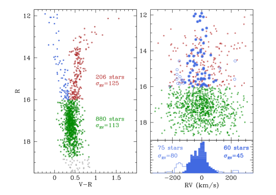
Figure 5: left: CMD of the global targets sampled in p0m2 color-coded according to their evolutionary phase. Red and blue symbols refer to the bona-fide bulge-RGB and disk-MS stars, respectively. For the bona-fide sample, the total number of stars and their radial velocity dispersion are also given. Green circles mark either bulge- or disk-MS and MS-TO stars. Top right: heliocentric RV as a function of the star magnitude of all stars adopting the same color code as in the left panel. Blue solid symbols refer to disk-MS stars with $|RV|<120$ km/s. Bottom right: heliocentric radial velocity distribution of disk-MS stars. The velocity dispersion of the total disk-MS sample and of the sub-sample obtained after applying a cut at $|RV|<120$ km/s are given.

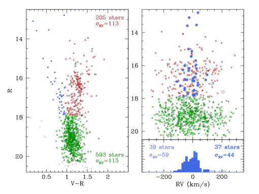
Figure 6: Same as Fig. 5 for m1p2 field.

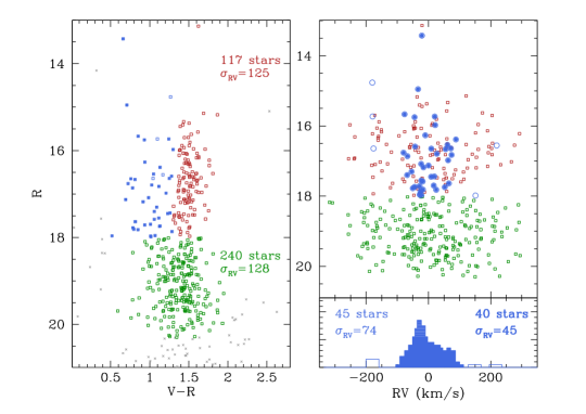
Figure 7: Same as Fig. 5 for p0p2 field.

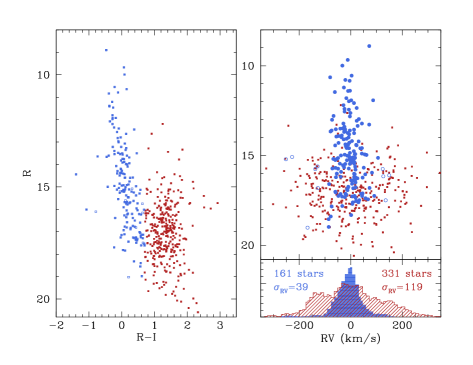
Figure 8: Same as Fig. 5 for p1m1 field. In this case the bulge MS falls below the limit magnitude, and therefore bulge RGB stars can be separated from disk MS stars by means of a simple color cut.

The RV distributions for all the sampled stars, in the 3 fields at $b=\pm 2^{\circ}$, are shown in Fig. 9. As demonstrated above, the best-fit to the observed velocity distribution in all fields is obtained with a combination of two Gaussian components with approximately the same mean ($(RV_{b}-RV_{d})\sim$10 km/s) but very different $\sigma$. The foreground disk stars contaminating the bulge sample have a velocity distribution with smaller dispersion (blue dashed line in Fig. 9). Specifically, we found the velocity dispersion of the disk population along the line of sight towards p0m2, m1p2 and p0p2 fields to be $\sigma$=45, 40, 35 km/s, respectively. These values agree with the APOGEE findings (Ness et al., 2016) for disk stars in the foreground of the bulge, within a distance of 3 kpc, as well as those reported by Robin et al. (2017) for thick disk stars in the solar neighbourhood. In Table 3 we list the mean heliocentric RV and velocity dispersion measured for the bulge stars as obtained from the best-fit to the velocity distribution of the global sample. In addition, following the prescription of Ness et al. (2013b), we provide the mean galactocentric radial velocity ($V_{GC}$) by correcting the mean heliocentric value for the Sun motion with respect to the Galactic center.

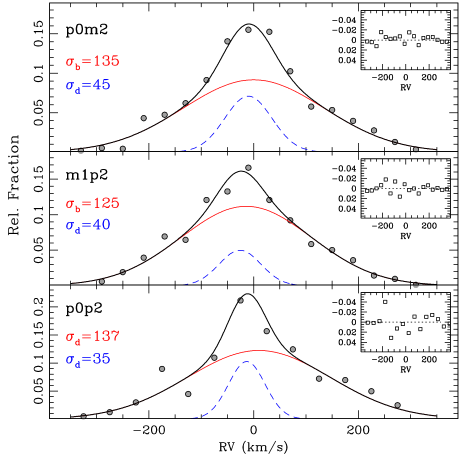
Figure 9: Normalised heliocentric radial velocity distribution function for all sampled stars observed in the p0m2 (top panel), m1p2 (middle panel) and p0p2 (bottom panel) fields. The best-fit to the velocity distribution (solid black line) is obtained by using a combination of two gaussian (red and blue solid lines) functions whose sigma are also reported in each panel. The residuals of the best-fit are shown for each field in the insets.

Table 3: Mean heliocentric and galactocentric radial velocity, and velocity dispersion measured for the bulge stars in the observed fields

Field	$<V_{Helio}>$	$<V_{GC}>$	$\sigma$	Nb/Ntot Ntot
	(km/s)	(km/s)	(km/s)	(%)
p0m2	0 $\pm$ 4.4	+9.8	135 $\pm$ 3.1	79.5	1203
m1p2	$-$14 $\pm$ 4.6	$-$8.8	125 $\pm$ 3.3	87.5	861
p0p2	10 $\pm$ 7.5	19.2	137 $\pm$ 5.3	82.4	496
p1m1	1 $\pm$ 6.6	14.7	119 $\pm$ 4.7	67.3	502

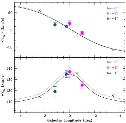
Figure 10: Mean galactocentric radial velocity (top) and velocity dispersion (bottom) as a function of the Galactic longitude, for different latitude as listed in the labels. Big color symbols refer to fields observed with MUSE, whereas small crosses mark the innermost GIBS fields at $b=-2^{\circ}$ (black) and $b=-1^{\circ}$ (grey). The solid lines represent the expected trend of the radial velocity and velocity dispersion according to the maps derived in Zoccali et al. (2014, equations 1 and 2). Error bars are derived from the sampling.

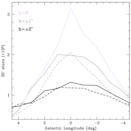
Figure 11: Profile of the stellar projected density, as traced by RC stars, in the inner few degrees of the Galactic bulge, from Valenti et al. (2016). The figure is a zoom of their Fig. 4, with solid/dashed lines referring to negative/positive latitudes, respectively.

5 Discussion and Conclusions

We have measured radial velocities for several hundreds bulge stars in each of four fields located within $l=\pm 1.5^{\circ}$ and $b=\pm 2^{\circ}$, with the IFU spectrograph MUSE@VLT. All the fields are confined within a projected radius of 280 parsecs from the Galactic center, assuming the latter at 8 kpc from the Sun.

The aim of this work is to assess the presence of a large peak in velocity dispersion in this inner region of the Galaxy, previously identified by Zoccali et al. (2014) based on GIBS survey, and to constrain its shape (see Fig. 1 for a zoom of the inner region of the velocity dispersion map derived in that work). Figure 10 (bottom) shows the central velocity dispersion peak as measured in the five innermost GIBS fields (black and gray small points, at $b=-2^{\circ}$ and $b=-1^{\circ}$, respectively) and as predicted in other Galactic positions according to the interpolated surface derived in that paper (black and grey curves). The curve was assumed to be symmetric above and below the Galactic plane, therefore the prediction for negative or positive latitude is identical by definition. The upper panel of Fig. 10 shows the same but for the radial velocity.

The new values derived in the present work are plotted in Fig. 10 with large colored symbols. They confirm both the presence of the central velocity dispersion peak, and its absolute value, reaching $\sigma V_{\rm GC}$ $\sim$ 140 km/s at its center. We also confirm that the peak is symmetric above and below the plane, as the two measurements at ($l,b$)=(0^∘,-2^∘) and (0^∘,+2^∘) are mutually consistent. With the present data we cannot constrain the latitude extension of the peak better than what was done in Zoccali et al. (2014), who found that the peak would disappear at the latitude of Baade’s window ($b=-4^{\circ}$). We can however constrain the longitude extension of the peak, which we show to be at least as narrow as predicted by GIBS in longitude. In fact, the new fields at $l=\pm 1^{\circ}$ have a velocity dispersion that is lower than the prediction of the GIBS maps.

In Valenti et al. (2016) we have derived maps of stellar projected density and stellar mass from star counts in the VVV PSF catalogues, using red clump stars as tracers of the total number of stars (and stellar mass). We found the presence of a peak in stellar density in the inner few degrees of the Galaxy, that is reproduced here in Fig. 11. This demonstrates that the sudden increase in velocity dispersion is likely due to the presence of a large concentration of stars (/mass) in the inner Galaxy. The Galactic position and spatial extension of the peak roughly coincides with the sigma peak characterised here, even if its detailed shape is somehow different. In particular, while the sigma peak is still rather sharp at $b=\pm 2^{\circ}$, the peak in star counts is already very shallow at these latitudes. On the other hand, while the conversion from observed velocity and mass requires dynamical modelling, as it requires hypothesis on the orbit distribution and their possible anisotropy, it is qualitatively expected that the effect of a mass concentration on the stellar velocity is felt down to some distance from the mass source. Hence it is not surprising that the sigma peak is more spatially extended than the stellar density peak.

One thing that deserves further study is the fact that, according to Zoccali et al. (2017), metal-poor stars slightly dominate the stellar density at $b=1^{\circ}$ (their Fig. 7), but the velocity dispersion is higher for metal-rich stars, in the same field (their Fig. 12). This is a clear evidence that the conversion between velocity dispersion and mass involves at least another parameter (the anisotropy of the orbit distribution) and that this parameter is different for metal-poor and metal-rich stars.

The data provided here should be included in the (chemo)-dynamical models of the Galaxy (e.g., Di Matteo et al., 2015; Debattista et al., 2017; Portail et al., 2017; Fragkoudi et al., 2018) in order to properly take into account the mass distribution of the inner few degrees of the Milky Way.