Computing the Helmholtz Capacitance of Charged Insulator-Electrolyte Interfaces from the Supercell Polarization

Abstract

Supercell modelling of an electrical double layer (EDL) at electrified solid-electrolyte interfaces is a challenge. The net polarization of EDLs arising from the fixed chemical composition setup leads to uncompensated EDLs under periodic boundary condition and convolutes the calculation of the Helmholtz capacitance [Zhang and Sprik, Phys. Rev. B, 94, 245309 (2016)]. Here we provide a new formula based on the supercell polarization at zero electric field $\bar{E}=0$ to calculate the Helmholtz capacitance of charged insulator-electrolyte interfaces and validate it using atomistic simulations. Results are shown to be independent of the supercell size. This formula gives a shortcut to compute the Helmholtz capacitance without locating the zero net charge state of EDL and applies directly to any standard molecular dynamics code where the electrostatic interactions are treated by the Ewald summation or its variants.

Charged insulating oxides-electrolyte interfaces are commonly found in electro/geochemistry Westall and Hohl (1980); Ardizzone and Trasatti (1996); Israelachvili (2011). The charge of insulator surface comes from the acid-base chemistry. It is negatively charged because of the deprotonation of the adsorbed water, when pH goes above the point of zero charge (PZC). On the other hand, it can become positively charged by protonation when pH goes below PZC Ardizzone and Trasatti (1996). The charged insulator surface will naturally polarize surrounding water molecules and attract counterions from the electrolyte to form the electric double layer (EDL). The most important quantity to characterize EDL is its capacitance.

For insulating oxides (or semiconducting oxides at the flatband condition) Nozik and Memming (1996); Grätzel (2001), the capacitance can be written as two distinct components connected in series:

$$1/C_{\text{EDL}}=1/C_{\text{H}}+1/C_{\text{GC}}$$ (1)

The first component $C_{\text{H}}$ is the Helmholtz capacitance due to the chemisorption of hydroxide groups or protons and the attraction of counterions. The dimension of $C_{\text{H}}$ is of a molecular size. The second component $C_{\text{GC}}$ called Gouy-Chapman capacitance, stems from the diffusive electrolyte and depends on the ionic strength. Because the diffuse ionic layer has a much higher capacitance and the inverse $C_{\text{GC}}$ term turns to be rather small, this makes the Helmholtz capacitance $C_{\textrm{H}}$ the leading term (similar to the dead-layer effect at water interfaces Zhang (2018)) and the focus of this study.

Computing $C_{\textrm{H}}$ may not be as easy as it seems. Under periodic boundary condition (PBC), two insulator-electrolyte interfaces can be charged up either symmetrically (same amounts and types of surface charges)  Cheng and Sprik (2014); Dewan et al. (2014); Sultan, Hughes, and Walsh (2014); Parez, Předota, and Machesky (2014); Hocine et al. (2016); Khatib et al. (2016) or asymmetrically (same amounts but opposite types of surface charges) Guerrero-García and Olvera de la Cruz (2013); Pfeiffer-Laplaud and Gaigeot (2016). However, only in the asymmetric setup, the chemical composition can be kept fixed at different surface charge densities, which satisfies the actual experimental conditions. In the asymmetric setup (Fig. 1a), supercell contains two parallel EDLs and a net polarization. As a consequence, each EDL is not fully compensated under PBC. This can be easily inferred from the electrostatic potential profile of the model system (Fig. 1b), where there is an electric field in the insulator region (Here we simply used vacuum for the proof-of-concept). According to Gauss’s theorem, a finite field means the enclosed body (an EDL for this case) bears a net charge. This net charge in EDLs is the manifestation of a finite-size error which plagues the computation of the Helmholtz capacitance.

Built on finite field methods developed by Stengel, Spaldin and Vanderbilt (SSV) Stengel, Spaldin, and Vanderbilt (2009); Stengel, Vanderbilt, and Spaldin (2009) for ferroelectric systems and extended later to finite-temperature simulations Zhang and Sprik (2016a); Zhang, Hutter, and Sprik (2016), we have proposed and validated two methods to compute the size-independent Helmholtz capacitance of EDLs of charged insulator-electrolyte interfaces under PBC Zhang and Sprik (2016b). The first one is based on constant electric field $\bar{E}$ simulations. By locating the zero net charge (ZNC) state of EDL, the corresponding external field $\bar{E}$ gives directly the Helmholtz capacitance of EDLs Zhang and Sprik (2016b). Subsequently, this method was extended to study charge compensation between polar surfaces and electrolyte solution Sayer, Zhang, and Sprik (2017). The second one is based on constant electric displacement $\bar{D}$ simulations. The differential of the itinerant polarization with respect to the imposed surface charge density at constant $\bar{D}$ gives an efficient estimation of the overall Helmholtz capacitance of EDLs Zhang and Sprik (2016b).

These two methods were devised from our analysis of a Stern-like model as the continuum counterpart of the atomistic system. In the second method based on constant $\bar{D}$ simulations, one gets the Helmholtz capacitance $C_{\textrm{H}}$ without locating ZNC state of EDL Zhang and Sprik (2016b). This suggests that it should be possible to derive the corresponding formula without relying on the Stern-like continuum model. In this Letter, we rederive the method for calculating the Helmholtz capacitance at constant $\bar{D}$ and show that this leads to a new formula to compute the Helmholtz capacitance using the supercell polarization at $\bar{E}=0$ (i.e. the standard Ewald boundary condition) through thermodynamics relations. This new formula is then verified by molecular dynamics (MD) simulation based on a simple point-charge (SPC)-like model of the charged insulator-electrolyte system. The resulting Helmholtz capacitance is shown to be independent of the supercell size and in excellent agreement with that obtained from constant electric displacement $\bar{D}$ simulations Zhang and Sprik (2016b).

What we start with is the hybrid SSV constant $\bar{D}$ Hamiltonian, which can be derived either from the thermodynamics argument originally Stengel, Spaldin, and Vanderbilt (2009) or from a current dependent Lagrangian as shown recently Sprik (2018):

$$H_{D}\left(v,\bar{D}\right)=H_{\mathrm{PBC}}(v)+\frac{\mathit{\Omega}}{8\pi}\left(\bar{D}-4\pi P(v)\right)^{2}$$ (2)

where $P$ is the itinerant polarization in the direction of $\bar{D}$ (See Secs. IV B and IV C in Ref.  Zhang and Sprik (2016b) for the elaboration), which is formally defined as a time integral of the volume integral of current  King-Smith and Vanderbilt (1993); Resta (1994); Resta and Vanderbilt (2007); Caillol, Levesque, and Weis (1989a, b); Caillol (1994). $\Omega$ is the supercell volume and $v=(\mathbf{r}^{N},\mathbf{p}^{N})$ stands for the collective momenta and position coordinates of the $N$ particles in the system. The bar over $D$ emphasizes that it is a variable instead of an observable. “Hybrid” means the field is only applied in the direction perpendicular to the surface.

The extended Hamiltonian $H_{D}\left(v,\bar{D}\right)$ of Eq. 2 generates a field dependent partition function

$$Z_{D}(\bar{D})=\int d\nu\exp[-\beta H_{D}\left(v,\bar{D}\right)]$$ (3)

$\beta=1/k_{\mathrm{B}}T$ is the inverse temperature. The combinatorial prefactor $1/(h^{3N}N!)$ has been omitted.

The expectation value of an observable $X$ is

$$\langle X\rangle=\int d\nu\frac{X\exp\left[-\beta H_{D}\left(\nu,\bar{D}\right)\right]}{Z_{D}(\bar{D})}$$ (4)

The electric displacement $\bar{D}$ is related to the electric field $E$ according to the definition:

$$\bar{D}=E+4\pi P$$ (5)

This leads to the expectation value of the voltage difference $\Delta V$ crossing the supercell as:

$$\langle\Delta V\rangle=-\langle E\rangle L=-(\bar{D}-4\pi\langle P\rangle)L$$ (6)

where $L$ is the dimension of the supercell in the $z$ direction which is along the surface normal.

Then, the overall capacitance according to the definition is:

$$C_{\textrm{tot}}=\frac{C_{H}}{2} = \left(\frac{\partial\sigma_{0}}{\partial\langle\Delta V\rangle}\right)_{\bar{D}}$$ (7)

$$= \left(\frac{\partial\sigma_{0}}{-\partial(\bar{D}-4\pi\langle P\rangle)L}\right)_{\bar{D}}$$ (8)

$$= \frac{1}{4\pi L}\left(\frac{\partial\sigma_{0}}{\partial\langle P\rangle}\right)_{\bar{D}}$$ (9)

Here we assume again that two EDLs connected in series have the same Helmholtz capacitance $C_{\textrm{H}}$ (Fig. 1a). In other words, $C_{\textrm{H}}$ is the average Helmholtz capacitance at a surface charge density $|\sigma_{0}|$. We notice that Eq. 9 is the same differential formula for the capacitance of the Helmholtz capacitance $C_{\textrm{H}}/2$ at constant $\bar{D}$, as derived from the linear electric equation of state using the Stern-like continuum model in our previous work Zhang and Sprik (2016b).

Because $\bar{D}$ and $\bar{E}$ are thermodynamic conjugate variables, this allows us to find out the corresponding relation of Eq. 9 at $\bar{E}$. The procedure we took is similar to that used to establish the thermodynamic relation between heat capacities at constant volume and at constant pressure.

First, we introduce following two expressions:

$$\left(\frac{\partial\sigma_{0}}{\partial\bar{D}}\right)_{P} = -\left(\frac{\partial\sigma_{0}}{\partial P}\right)_{\bar{D}}\left(\frac{\partial P}{\partial\bar{D}}\right)_{\sigma_{0}}$$ (10)

$$\left(\frac{\partial\sigma_{0}}{\partial\bar{E}}\right)_{P} = -\left(\frac{\partial\sigma_{0}}{\partial P}\right)_{\bar{E}}\left(\frac{\partial P}{\partial\bar{E}}\right)_{\sigma_{0}}$$ (11)

The ratio between them leads to:

$$\left(\frac{\partial\sigma_{0}}{\partial P}\right)_{\bar{D}}\left(\frac{\partial P}{\partial\sigma_{0}}\right)_{\bar{E}} = \left(\frac{\partial\bar{D}}{\partial\bar{E}}\right)_{\sigma_{0}}\left(\frac{\partial\bar{E}}{\partial\bar{D}}\right)_{P}$$ (12)

$$= \epsilon_{\perp}\left(\frac{\partial\bar{E}}{\partial\bar{D}}\right)_{P}$$ (13)

Here $\epsilon_{\perp}$ is the overall dielectric constant of the heterogenous system in the direction perpendicular to the surface and the subscript $\sigma_{0}$ of $\epsilon_{\perp}$ is omitted.

Then, the second term on the right hand side of Eq. 13 can be rewritten as,

$$\left(\frac{\partial\bar{E}}{\partial\bar{D}}\right)_{P} = \left(\frac{\partial\bar{E}}{\partial\sigma_{0}}\right)_{P}\left(\frac{\partial\sigma_{0}}{\partial\bar{D}}\right)_{P}$$ (14)

$$= \left(\frac{\partial\bar{E}}{\partial\sigma_{0}}\right)_{P}\left(\frac{\partial\sigma_{0}}{\partial(\bar{E}+4\pi P)}\right)_{P}$$ (15)

$$= \left(\frac{\partial\bar{E}}{\partial\sigma_{0}}\right)_{P}\left(\frac{\partial\sigma_{0}}{\partial\bar{E}}\right)_{P}$$ (16)

$$= 1$$ (17)

Combining Eq. 13 and Eq. 17, we obtain a key intermediate result:

$$\left(\frac{\partial\sigma_{0}}{\partial P}\right)_{\bar{D}}\left(\frac{\partial P}{\partial\sigma_{0}}\right)_{\bar{E}}=\epsilon_{\perp}$$ (18)

Inserting Eq. 18 into Eq. 9, one ends up with the desired relation:

$$\frac{C_{H}}{2}=\frac{\epsilon_{\perp}}{4\pi L}\left(\frac{\partial\sigma_{0}}{\partial\langle P\rangle}\right)_{\bar{E}}$$ (19)

This is the corresponding differential formula for the overal Helmholtz capacitance at constant $\bar{E}$.

For the system at $\bar{E}=0$ and under PBC, it is known from the linear response theory that Neumann (1983):

$$\epsilon_{\perp}=\left(\frac{\partial\langle P\rangle}{\partial\bar{E}}\right)_{\bar{E}=0}+1=4\pi\beta\mathit{\Omega}\left(\langle P^{2}\rangle_{\bar{E}=0}-\langle P\rangle^{2}_{\bar{E}=0}\right)+1$$ (20)

Since $\langle P\rangle=0$ for $\sigma_{0}=0$, therefore, the equation for computing $C_{\textrm{H}}$ is simply:

$$\frac{C_{\textrm{H}}}{2} = \frac{\epsilon_{\perp}}{4\pi L}\frac{\sigma_{0}}{\langle P\rangle}_{\bar{E}=0}$$ (21)

$$= \frac{\sigma_{0}\left[4\pi\beta\mathit{\Omega}\left(\langle P^{2}\rangle_{\bar{E}=0}-\langle P\rangle^{2}_{\bar{E}=0}\right)+1\right]}{4\pi L\langle P\rangle_{\bar{E}=0}}$$ (22)

Eq. 22 is the main result of this work, where the polarization fluctuation is a necessary piece of information for computing the Helmholtz capacitance at $\bar{E}=0$, i.e. the standard Ewald boundary condition, for the generic system showed in Fig. 1a.

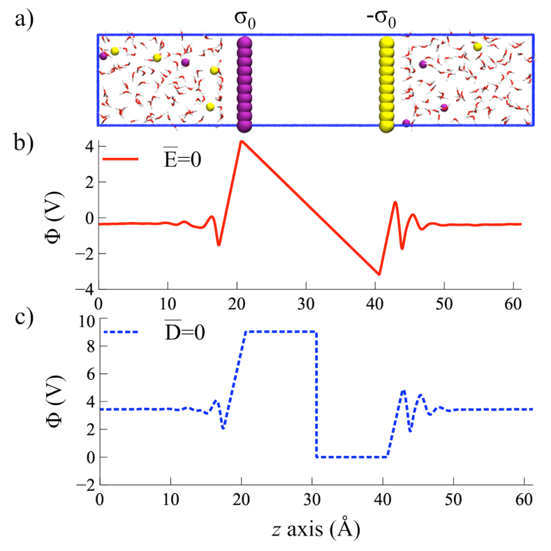
Figure 1: a) Periodic model of two complementary charged insulator-electrolyte interfaces used as the model system in this study. The charged insulator is modelled as a pair of rigid atomic walls with opposite charge separated by a vacuum region (the insulator). The surface charge is uniformly distributed over area $A$ with a charge density $\sigma_{0}$. Positive charges are in purple and negative charges are in yellow. b) The electrostatic potential profile $\Phi(z)$ averaged over the perpendicular $x$ and $y$ directions at $\bar{E}=0$ and $A\sigma_{0}=2e$; c) The electrostatic potential profile $\Phi(z)$ averaged over the perpendicular $x$ and $y$ directions at $\bar{D}=0$ and $A\sigma_{0}=2e$.

To test whether this formula gives a size-independent estimator of the Helmholtz capacitance, we have performed MD simulation of a SPC-like model, which is familiar from many studies of electrode-electrolyte interfaces Spohr (1999); Dimitrov and Raev ; Fedorov and Kornyshev (2008); Zarzycki, Kerisit, and Rosso (2010); Lynden-Bell, Frolov, and Fedorov (2012); Sultan, Hughes, and Walsh (2014); Parez, Předota, and Machesky (2014); Dewan et al. (2014); Hocine et al. (2016). The electrolyte consists of 202 water molecules, 5 Na⁺ and 5 Cl^- ions. The oppositely charged insulator slab was modelled as two rigid uniformly charged atomic walls plus a vacuum slab in between as the insulator. The simulation box is rectangular. The length in $x$ and $y$ direction is 12.75 Å  and the length in $z$ direction varies from 61.24 Å to 121.24 Å depending on the thickness of the insulator (vacuum in this case). Water are described by the SPC/E model potential Berendsen, Grigera, and Straatsma (1987) and alkali metal ions are modelled as point charge plus Lennard-Jones potential using the parameters from Jung and Cheatham Joung and T E Cheatham (2008); Zhang et al. (2010). The van der Waals parameters of the particle in the rigid wall were simply chosen to be the same as those of oxygen atom. The MD integration time step is 2 fs and trajectories were accumulated for 10ns for each combination of the charge density and the electric boundary condition. The electrostatics was computed using Particle Mesh Ewald (PME) scheme Darden, York, and Pedersen (1993). Short-range cutoffs for the Van der Waals and Coulomb interaction in direct space are 6 Å. The temperature was controlled by a Nosé-Hoover chain thermostat set at 298K Martyna, Klein, and Tuckerman (1992). These technical setting are the same as in the previous work Zhang and Sprik (2016b) and all simulations were done with a modified version of GROMACS 4 package Hess et al. (2008). In the case of $\bar{D}=0$ simulation, we used the hybrid constant $\bar{D}$ Hamilton shown in Eq. 2. This implies a static and homogenous $\bar{D}$ field was only applied in the direction perpendicular to the surface (i.e. $z$ direction) over the whole simulation box. Regarding the itinerant polarization $P$, it differs from the conventional cell polarization $P^{\textrm{cell}}(t)=\frac{1}{\Omega}\sum_{i}^{\textrm{cell}}q_{i}\textrm{nint}(L^{-1}z_{i}(t))$ by preserving the continuity of time-integrated current King-Smith and Vanderbilt (1993); Resta (1994); Resta and Vanderbilt (2007); Caillol, Levesque, and Weis (1989a, b); Caillol (1994). This means that the iternative polarization $P$ is continuous throughout the trajectory and particles need to be tracked from t=0 if they leave the MD supercell when computing the polarization. From the iternative polariztion $P$, one can also compute the overal dielectric constant $\epsilon_{\perp}$ following Eq. 20 straightforwardly.

The polarization potential $4\pi L\langle P\rangle$ has the same unit as the voltage and that is what we plotted in Fig. 2a. As shown in the Figure, the polarization potential at $\bar{E}=0$ has a linear relation with respect to the imposed charge density $\sigma_{0}$. The slope which is directly related to the Helmholtz capacitance has a strong size dependence of the supercell. This confirms that the insulator also contributes to the total capacitance because of the existing field in the insulator region under PBC (Fig. 1b). This is the finite-size error that we want to remove.

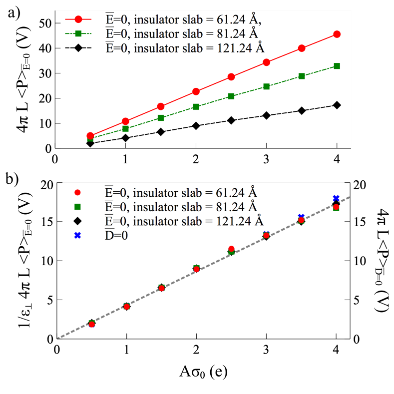
Figure 2: a) The polarization potential $4\pi L\langle P\rangle$ (in volt) as a function of the imposed surface charge $A\sigma_{0}$ of the charged insulator-electrolyte system for three different insulator slab sizes at $\bar{E}$=0. $L$ is the the box length in $z$ direction, perpendicular to the surface; b) The overall dielectric constant $\epsilon_{\perp}$ weighted polarization potential $1/\epsilon_{\perp}4\pi L\langle P\rangle$ (in volt) as a function of the imposed surface charge $A\sigma_{0}$ for the same system at $\bar{E}=0$. This should be compared to the polarization potential $4\pi L\langle P\rangle$ (in volt) as a function of the imposed surface charge density $A\sigma_{0}$ at $\bar{D}=0$. $\epsilon_{\perp}$ was computed according to Eq. 20 for the system of different surface charge density and insulator slab size.

Following Eq. 21, we weighted the polarization potential $4\pi L\langle P\rangle$ at $\bar{E}=0$ by the overall dielectric constant $\epsilon_{\perp}$ and results are shown in Fig. 2b. As seen in the Figure, data points for difference sizes of supercell at the same charge density $\sigma_{0}$ superimpose with each other. By fitting these data to a linear function passing the origin, one can obtain the slope which gives the inverse of the Helmholtz capacitance. To check the consistency, we also computed the polarization potential $4\pi L\langle P\rangle$ at $\bar{D}=0$ as the reference (Fig. 1c). One needs to pay attention that the D value which restores the ZNC state of EDL for the insulator centered supercell is subject to the modulation of the polarization quantum $4\pi e/A$, i.e. $D^{n}_{\text{ZNC}}=n4e\pi/A$  Zhang and Sprik (2016b) where $n$ is an integer. For the supercell shown in Fig. 2a with $A\sigma_{0}=2e$, $D^{n}_{\text{ZNC}}=0$.

As shown in Fig. 2b, the polarization potential $4\pi L\langle P\rangle$ at $\bar{D}=0$ at the same charge density are spot on the weighted polarization potential $1/\epsilon_{\perp}4\pi L\langle P\rangle$ at $\bar{E}=0$. This suggests both Eq. 19 and Eq. 9 give the same result for the Helmholtz capacitance, which is independent of the the system size.

In our previous work Zhang and Sprik (2016b), it was demonstrated that a finite $\bar{E}$ field can be applied to cancel out the existing field in the insulator region and to restore the point of ZNC of EDLs. Subsequently, the Helmholtz capacitance can be obtained from the value of the restoring field at ZNC as Zhang and Sprik (2016b):

$$V_{\textrm{znc}}=-L\bar{E}_{\textrm{znc}}=2\sigma_{0}/C_{\textrm{H}}$$ (23)

Putting Eq. 23 and Eq. 22 together, we obtain a new estimator of the external potential needed to restore ZNC state just using the supercell polarization at zero electric field:

$$V_{\textrm{znc}}=-L\bar{E}_{\textrm{znc}}=\frac{4\pi L\langle P\rangle_{\bar{E}=0}}{4\pi\beta\mathit{\Omega}\left(\langle P^{2}\rangle_{\bar{E}=0}-\langle P\rangle^{2}_{\bar{E}=0}\right)+1}$$ (24)

For the surface charge $A\sigma_{0}=2.0e$, the above formula gives an estimate of $V_{\textrm{znc}}$ as 9.0 V. This value should be compared to 8.9 V as reported previously for the same SPC-like system by monitoring the net charge of EDL $Q_{\textrm{net}}$ as a function of the applied voltage $V_{\textrm{ext}}$ Zhang and Sprik (2016b). Therefore, Eq. 24 is also validated.

Like its constant $\bar{D}$ variant in Eq. 9, Eq. 22 does not require an additional vacuum slab in the first place, which is a relief for plane-wave based electronic structure calculation. Here, the main advantage of using this formula to compute the Helmholtz capacitance is that it works directly with any standard MD code in which the electrostatic interactions are treated by the Ewald summation (or its variants). This was achieved by introducing the overal dielectric constant $\epsilon_{\perp}$ which absorbs the finite-size effect. Thus, it would be interesting in future works to look closer at the role of $\epsilon_{\perp}$ in supercell modeling of heterogenous systems. Nevertheless, it is worth to mention that Eq. 22 only provides a shortcut to compute the Helmholtz capacitance and a finite field (either $\bar{E}$ or $\bar{D}$) is still required to restore the ZNC state of EDL in supercell modeling of charged insulator-electrolyte interfaces.

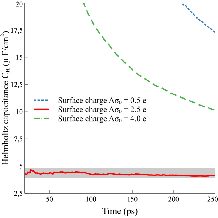
Figure 3: The running average of the Helmholtz capacitance $C_{\text{H}}$ calculated from the supercell polarization using Eq. 22 at difference surface charges with the smallest box length used in this work (i.e. $L=61.24$ Å). All simulations were done using the same initial configuration extracted from an equilibrated system at surface charge $A\sigma_{0}=2.0~{}e$ and with the same chemical composition. The shaded area indicates $\pm 10$% deviations from the supposed $C_{\text{H}}$ value of this SPC-like model.

Before closing this Letter, it is necessary to discuss the convergence of the Helmholtz capacitance computed from the supercell polarization. According to the classical Debye theory, switching the electric boundary condition from constant $\bar{E}$ to constant $\bar{D}$ would lead to a speed-up of the relaxation time of the macroscopic polarization by a factor comparable to the dielectric constant of the medium. This was indeed seen in the simulation of bulk liquid water Zhang and Sprik (2016a). As a consequence, the convergence of $C_{\text{H}}$ of charged solid-liquid interfaces can be achieved within 50 ps by using constant $\bar{D}$ simulations (i.e. Eq. 9) and a SPC-like model (See Fig. 11 in Ref. Zhang and Sprik (2016b)). Instead, Eq. 22 uses the standard Ewald boundary condition ($\bar{E}=0$) and relies on the overal dielectric constant $\epsilon_{\perp}$ which can have the same notoriously slow convergence (few nanoseconds) as what we knew for polar liquids (See Ref. Zhang, Hutter, and Sprik (2016) and reference therein). However, the convergence Eq. 22 of can be achieved within tens of picoseconds in practice if the system was equilibrated at a chosen surface charge nearby the target value (Fig. 3). This leverages the feasibility of applying Eq. 22 in density functional theory based MD simulations.