Randomly weighted CNNs for (music) audio classification

Abstract

The computer vision literature shows that randomly weighted neural networks perform reasonably as feature extractors. Following this idea, we study how non-trained (randomly weighted) convolutional neural networks perform as feature extractors for (music) audio classification tasks. We use features extracted from the embeddings of deep architectures as input to a classifier – with the goal to compare classification accuracies when using different randomly weighted architectures. By following this methodology, we run a comprehensive evaluation of the current deep architectures for audio classification, and provide evidence that the architectures alone are an important piece for resolving (music) audio problems using deep neural networks.

1 MOTIVATION – FROM PREVIOUS WORKS

Some intriguing properties of deep neural networks are periodically showing up in the scientific literature. Examples of those are: (i) perceptually non-relevant signal perturbations that dramatically affect the predictions of an image classifier [12, 49]; (ii) although there is no guarantee of converging to a global minima that might generalize, image classification models perform well with unseen data [25, 14]; or (iii) non-trained deep neural networks are able to perform reasonably well as image feature extractors [43, 51, 41]. In this work, we exploit one of the above listed properties (iii) to evaluate how discriminative deep audio architectures are before training.

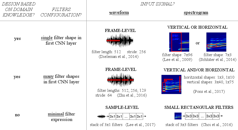
Figure 1: CNN front-ends for audio classification tasks – with examples of possible configurations for every paradigm.

Previous works already explored the idea of empirically studying the qualities of non-trained (randomly weighted) networks, but mainly in the computer vision field:

$\mathbf{\cdot}$ Saxe et al. [43] studied how discriminative are the architectures themselves by evaluating the classification performance of SVMs fed with features extracted from non-trained (random) CNNs.They showed that a surprising fraction of the performance in deep image classifiers can be attributed to the architecture alone. Therefore, the key to good performance lies not only on improving the learning algorithms but also in searching for the most suitable architectures. Further, they showed that the (classification) performance delivered by random CNN features is correlated with the results of their end-to-end trained counterparts – this result means, in practice, that one can bypass the time-consuming process of learning for evaluating a given architecture. We build on top of this result to evaluate current CNN architectures for audio classification.

$\mathbf{\cdot}$ Rosenfeld and Tsotsos [41] fixed most of the model’s weights to be random, and only allowed a small portion of them to be learned. By following this methodology, they showed a small decrease in image classification performance when these models were compared to their fully trained counterparts. Further, the performance of their non fully-trained models can be summarized as follows:

DenseNet[17] $\gg$ ResNet[15] $>$ VGG[48] $\gg$ AlexNet[25]

What matches previous works reporting how these (fully trained) models perform[17, 15, 48], confirming the performance correlation between randomly weighted models and their trained counterparts found by Saxe et al. [43]

$\mathbf{\cdot}$ Adebayo et al. [1] empirically assessed the local explanations of deep image classifiers to find that randomly weighted models produce explanations similar to those produced by models with learned weights. They conclude that the architectures introduce a strong prior which affects the learned (and not learned) representations.

$\mathbf{\cdot}$ Ulyanov et al. [51] also showed that the structure of a network (the non-trained architecture) is sufficient to capture useful features for the tasks of image denoising, super-resolution and inpainting. They think of any designed architecture as a hand-crafted model where prior information is embedded in the structure of the network itself. This way of thinking resonates with the rationale behind the family of audio models designed considering domain knowledge (see section 2) – what denotes that in both audio and image fields it exists the interest of bringing together the end-to-end learning literature and previous research.

Few related works exist in the audio field – and every randomly weighted neural network we found in the audio literature was a mere baseline [7, 24, 2]. Inspired by previous computer vision works, we study which audio architectures work the best via evaluating how non-trained CNNs perform as feature extractors. To this end, we use the CNNs’ embeddings to construct feature vectors for a classifier – with the goal to compare classification performances when different randomly weighted architectures are used to extract features. To the best of our knowledge, this is the first comprehensive evaluation of randomly weighted CNNs for (music) audio classification.

Extreme learning machines (ELMs) [47, 32, 18] and echo state networks (ESNs) [19] are also closely related to our work. In short, ELMs are classification/regression modelsthat are based on a single-layer feed-forward neural network with random weights. They work as follows: first, ELMs randomly project the input into a latent space; and then, learn how to predict the output via a least-square fit. More formally, we aim to predict:

$$\hat{Y}=W_{2}\hskip 2.84526pt\sigma(W_{1}X),$$

where $W_{1}$ is the (randomly weighted) matrix of input-to-hidden-layer weights, $\sigma$ is the non-linearity, $W_{2}$ is the matrix of hidden-to-output-layer weights, and X represents the input. The training algorithm is as follows: 1) set $W_{1}$ with random values; 2) estimate $W_{2}$ via a least-squares fit:

$$W_{2}=\sigma(W_{1}X)^{+}Y$$

where ⁺ denotes the Moore-Penrose inverse. Since no iterative process is required for learning the weights, training is faster than stochastic gradient descent [18]. Provided that we process audio signals with randomly weighted CNNs, ELM-based classifiers are a natural choice for our study – so that all the pipeline (except the last layer) is based on random projections that are only constrained by the structure of the neural network. Although ELMs are not widely used by the audio community, they have been used for speech emotion recognition[13, 21], or for music audio classification[44, 29, 23]. ESNs differ from ELMs in that their random projections use recurrent connections. Given that the audio models we aim to study are not recurrent, we leave for future work using ESNs – see [45, 16] for audio applications of ESNs.

2 ARCHITECTURES

In this work we evaluate the most used deep learning architectures for (music) audio classification. In order to facilitate the discussion around these architectures, we divide the deep learning pipeline into two parts: front-end and back-end, see Figure 2. The front-end is the part that interacts with the input signal in order to map it into a latent-space, and the back-end predicts the output given the representation obtained by the front-end. Note that one can interpret the front-end as a “feature extractor” and the back-end as a “classifier”. Given that we compare how several non-trained (random) CNNs perform as feature extractors, and we will use out-of-the-box classifiers to predict the classes: this literature review focuses in introducing the main deep learning front-ends for audio classification.

Figure 2: The deep learning pipeline.

Front-ends — These are generally conformed by CNNs [9, 6, 53, 38, 39], since these can encode efficient representations by sharing weightsalong the signal. Figure 1 depicts six different CNN front-end paradigms, which can be divided into two groups depending on the used input signal: waveforms [9, 53, 27] or spectrograms [6, 38, 39]. Further, the design of the filters can be either based on domain knowledge or not. For example, one leverages domain knowledge when the frame-level single-shape front-end for waveforms is designed so that the length of the filter is set to be the same as the window length in a STFT [9]. Or for a spectrogram front-end, it is used vertical filters to learn spectral representations [26] or horizontal filters to learn longer temporal cues [46]. Generally, a single filter shape is used in the first CNN layer [9, 6, 26, 46], but some recent work reported performance gains when using several filter shapes in the first layer [53, 38, 39, 34, 36, 5]. Using many filters promotes a more rich feature extraction in the first layer, and facilitates leveraging domain knowledge for designing the filters’ shape. For example: a frame-level many-shapes front-end for waveforms can be motivated from a multi-resolution time-frequency transformperspective – with window sizes varying inversely with frequency [53]; or since it is known that some patterns in spectrograms are occurring at different time-frequency scales, one can intuitively incorporate many vertical and/or horizontal filters to efficiently capture those in a spectrogram front-end [38, 39, 36, 34]. As seen, using domain knowledge when designing the models allows to naturally connect the deep learning literature with previous relevant signal processing work. On the other hand, when domain knowledge is not used, it is common to employ a deep stack of small filters, e.g.: 3$\times$1 in the sample-level front-end used for waveforms [27, 52, 40], or 3$\times$3 in the small-rectangular filters front-end used for spectrograms [6]. These VGG-likemodels make minimal assumptions over the local stationarities of the signal, so that any structure can be learnt via hierarchically combining small-context representations.

3 METHOD

Our goal is to study which CNN front-ends work best via evaluating how non-trained models perform as feature extractors. Our evaluation is based on the traditional pipeline of features extraction + classifier. We use the embeddings of non-trained (random) CNNs as features: for every audio clip, we compute the average of each feature map (in every layer) and concatenate these values to construct a feature vector[7]. The baseline feature vector is constructed from 20 MFCCs, their $\Delta$s and $\Delta\Delta$s. We compute their mean and standard deviation through time, and the resulting feature vector is of size 120. We set the widely used MFCCs + SVM setup as baseline. To allow a fair comparison with the baseline, CNN models have $\approx$ 120 feature maps – so that the resulting feature vectors have a similar size as the MFCCs vector. Further, we evaluate an alternative configuration with more feature maps ($\approx$3500) to show the potential of this approach. Model’s description omit the number of filters per layer for simplicity – full implementation details are accessible online.

3.1 Features: randomly weighted CNNs

Except for the VGG model that uses ELUs as non-linearities [6, 8], the rest use ReLUs [10] – and we do not use batch normalization, see discussion in section 3.4. We use waveforms and spectrograms as input to our CNNs:

Waveform inputs — are of $\approx$ 29sec (350,000 samples at 12kHz) and the following architectures are under study:

$\cdot$ Sample-level: is based on a stack of 7 blocks that are composed by a 1D-CNN layer (filter length: 3, stride: 1) and a max-pool layer (size: 3, stride: 3) – with the exception of the input block which has no max-pooling and its 1D-CNN layer has a stride of 3 [27]. Averages to construct the feature vector are computed after every pooling layer, except for the first layer that are computed after the CNN.

$\cdot$ Frame-level many-shapes: consists of a 1D-CNN layer with five filter lengths: 512, 256, 128, 64, 32 [53]. Every filter’s stride is of 32 and we use same padding – to easily concatenate feature maps of the same size. Note that out of this single 1D-CNN layer, five feature maps (resulting of the different filter length convolutions) are concatenated. For that reason, every feature map needs to have the same (temporal) size. Since this model is single-layered and it might be in clear disadvantage when compared to the sample-level CNN, we increase its depth via adding three more 1D-CNN layers (length: 7, stride: 1) – where the last two layers have residual connections, and the penultimate layer’s feature map is down-sampled by two (MP x2), see Figure 3. Averages to construct the feature vector are calculated for each feature map after every 1D-CNN layer.

$\cdot$ Frame-level: consists of a 1D-CNN layer with a filter of length 512 [9]. Stride is set to be 32 to allow a fair comparison with the frame-level many-shapes architecture. As in frame-level many-shapes, we increase the depth of the model via adding three more 1D-CNN layers – as in Figure 3. Averages to construct the feature vector are calculated for each feature map after every 1D-CNN layer.

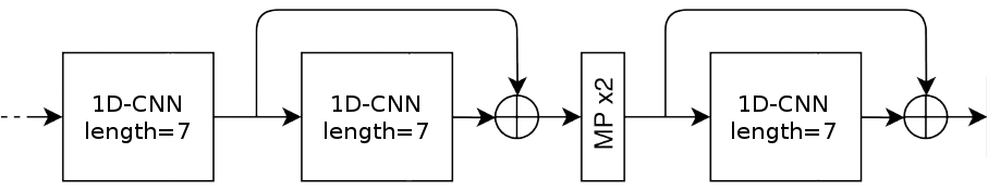
Figure 3: Additional layers for the frame-level & frame-level many-shapes architectures, similar as in [9, 37] – where MP stands for max pooling.

Spectrogram inputs — are set to be log-mel spectrograms(spectrograms size: 1376$\times$96, being $\approx$ 29sec of signal).Differently from waveform models, spectrogram architectures use no additional layers to deepen single-layered CNNs because these already deliver a reasonable classification performance. Unless we state the contrary, every CNN layer used for processing spectrograms is set to have stride 1. As for the frame-level many-shapes model, we use same padding when many filter shapes are used in the same layer. The following spectrogram models are studied:

$\cdot$ 7$\times$96: consists of a single 1D-CNN layer with filters of length 7 that convolve through the time axis [9]. As a result: CNN filters are vertical and of shape 7$\times$96. Therefore, these filters can encode spectral (timbral) representations. Averages to construct the feature vector are calculated for each feature map after the 1D-CNN layer.

$\cdot$ 7$\times$86: consists of a single 2D-CNN layer with vertical filters of shape 7$\times$86 [39, 36]. Since its vertical shape is smaller than the input (86$<$96), filters can also convolve through the frequency axis – what can be seen as “pitch shifting” the filter. Consequently, 7$\times$86 filters can encode pitch-invariant timbral representations [39, 36]. Further, since the resulting activations can carry pitch-related information, we max-pool the frequency axis to get pitch-invariant features (max-pool shape: 1$\times$11). Averages to construct the feature vector are calculated for each feature map after the max-pool layer.

$\cdot$ Timbral: consists of a single 2D-CNN layer with many vertical filters of shapes: 7$\times$86, 3$\times$86, 1$\times$86, 7$\times$38, 3$\times$38, 1$\times$38, see Figure 4 (top)[35, 11, 39]. These filters can also convolve through the frequency axis and therefore, these can encode pitch-invariant representations. Several filter shapes are used to efficiently capture different timbrically relevant time-frequency patterns, e.g.: kick-drums (can be captured with 7$\times$38 filters representing sub-band information for a short period of time), or string ensemble instruments (can be captured with 1$\times$86 filters representing spectral patterns spread in the frequency axis). Further, since the resulting activations can carry pitch-related information, we max-pool the frequency axis to get pitch-invariant features (max-pool shapes: 1$\times$11 or 1$\times$59). Averages to construct the feature vector are calculated for each feature map after the max-pool layer.

$\cdot$ Temporal: several 1D-CNN filters (of lengths: 165, 128, 64, 32) operate over an energy envelope obtained via mean-pooling the frequency-axis of the spectrogram, see Figure 4 (bottom). By computing the energy envelope in that way, we are considering high and low frequencies together while minimizing the computations of the model. Observe that this single-layered 1D-CNN is not operating over a 2D spectrogram, but over a 1D energy envelope – therefore no vertical convolutions are performed, only 1D (temporal) convolutions are computed. As seen, domain knowledge can also provide guidance to (effectively) minimize the computations of the model. Averages to construct the feature vector are calculated for each feature map after the CNN layer.

$\cdot$ Timbral+temporal: combines both timbral and temporal CNNs in a single (but wide) layer, see Figure 4[37]. Averages to construct the feature vector are calculated in the same way as for timbral and temporal architectures.

$\cdot$ VGG: is a computer vision model based on a stack of 5 blocks combining 2D-CNN layers (with small rectangular filters of 3$\times$3) and max-pooling (of shapes: 4$\times$2, 4$\times$3, 5$\times$2, 4$\times$2, 4$\times$4, respectively)[6]. Averages to construct the feature vector are computed after every pooling layer.

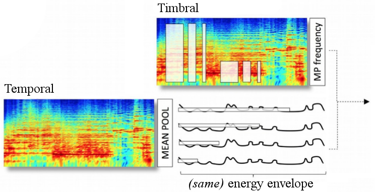
Figure 4: Timbral+temporal architecture. MP: max-pool.

As seen, studied architectures are representative of the audio classification state-of-the-art – introduced in section 2. For further details about the models under study: the code is accessible online, and a graphical conceptualization of the models is available in Figures 1, 3 and 4.

3.2 Classifiers: SVM and ELM

We study how several feature vectors (computed considering different CNNs) perform for a given set of classifiers: SVMs and ELMs. We discarded the use of other classifiers since their performance was not competitive when compared to those. SVMs and ELMs are hyper-parameter sensitive, for that reason we perform a grid search:

$\cdot$ SVM hyper-parameters: we consider both linear and rbf kernels. For the rbf kernel, we set $\gamma$ to: $2^{-3}$, $2^{-5}$, $2^{-7}$, $2^{-9}$, $2^{-11}$, $2^{-13}$, #features^-1; and for every kernel configuration, we try several C’s (penalty parameter): 0.1, 2, 8, 32. We use scikit-learn’s SVM implementation [33].

$\cdot$ ELM’s main hyper-parameter is the number of hidden units: 100, 250, 500, 1200, 1800, 2500. We use ReLUs as non-linearity, and we use a public ELM implementation.

3.3 Datasets: music and acoustic events

$\cdot$ GTZAN fault-filtered version [50, 22]. Training songs: 443, validation songs: 197, and test songs: 290 – divided in 10 classes. We use this dataset to study how randomly weighted CNNs perform for music genre classification.

$\cdot$ Extended Ballroom [30, 4] – 4,180 songs divided in 13 classes; 10 stratified folds are randomly generated for cross-validation. We use this dataset to study how randomly weighted CNNs classify rhythm/tempo classes.

$\cdot$ Urban Sound 8K [42] – 8732 acoustic events divided in 10 classes; 10 folds are already defined by the dataset authors for cross-validation. Since urban sounds are shorter than 4 seconds and our models accepts $\approx$ 29sec inputs, the signal is repeated to create inputs of the same length. We use this dataset to study how randomly weighted CNNs perform to classify natural (non-music) sounds.

3.4 Reproducing former results to discuss our method

Choi et al. [7] used random CNN features as baseline for their work, and found that (in most cases) these random CNN features perform better than MFCCs. Motivated by this result, we pursue this idea for studying how different deep architectures perform when resolving audio problems. To start, we first reproduce one of their experiments using random CNNs – under the same conditions: the GTZAN dataset is split in 10 stratified folds used for cross-validation, a VGG architecture with batch normalization is employed, and the classifier is an SVM. We found that results can vary depending on the batch size if, when computing the feature vectors, layers are normalized with the statistics of current batch (batch normalization). For example: if audio-features of the same genre are batch-normalized by the same factor, one can create an artificial genre cue that might affect the results. One can observe this phenomena in Figure 5, where the best results are achieved when all songs of the same genre fill a full batch (batch size of 100).We also observe that small batch sizes are harming the model’s performance – see in Figure 5 when batch sizes are set to 1 and 10. And finally, when batch normalization is not used, no matter what batch size we use that the results remain the same – ANOVA test with $H_{0}$ being that averages are equal(p-value=0.491). Since it is not desirable that performance depends on the batch size, and that the feature vector of an audio depends on other audios (that are present in the batch): we decided not to use batch normalization.

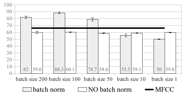
Figure 5: Random CNN features behavior when using (or not) batch normalization. Dataset: GTZAN, 10-fold cross-validation. Performance metric (%): average accuracies (and standard deviations) across 3 runs. Classifier: SVM.

4 Results

Figures show average accuracies across 3 runs for every feature type (listed on the right with the length of the feature vector in parenthesis). We use a t-test to reveal which models are performing the best – $H_{0}$: averages are equal.

4.1 GTZAN: music genre recognition

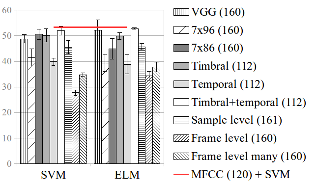
Figure 6: Accuracy (%) results for the GTZAN dataset with random CNN feature vectors of length $\approx$ 120.

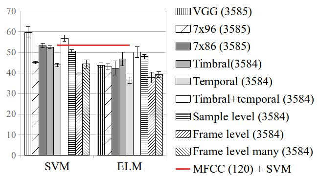
Figure 7: Accuracy (%) results for the GTZAN dataset with random CNN feature vectors of length $\approx$ 3500.

The sample-level waveform model always performs better than frame-level many-shapes (t-test: p-value$\ll$0.05). The two best performing spectrogram-based models are: timbral+temporal and VGG – with a remarkable performance of the timbral model alone. The timbral+temporal CNN performs better than VGG when using the ELM ($\approx$3500) classifier (t-test: p-value=0.017); but in other cases, both models perform equivalently (t-test: p-value$>$0.05). Moreover, the 7x86 model performs better than 7x96 when using SVMs (t-test: p-value$<$0.05), but when using ELMs: 7x96 and 7x86 perform equivalently (t-test: p-value$\gg$0.05). The best VGG and timbral+temporal models achieve the following (average) accuracies: 59.65% and 56.89%, respectively – both with an SVM ($\approx$3500) classifier. Both models outperform the MFCCs baseline: 53.44% (t-test: p-value$<$0.05), but these random CNNs perform worse than a CNN pre-trained with the Million Song Dataset: 82.1% [28]. Finally, note that although timbral and timbral+temporal models are single-layered, these are able to achieve remarkable performances – showing that single-layered spectrogram front-ends (attending to musically relevant contexts) can do a reasonable job without paying the cost of going deep [39, 36]. Thus meaning, e.g., that the saved capacity can now be employed by the back-end to learn (some more) representations.

4.2 Extended Ballroom: rhythm/tempo classification

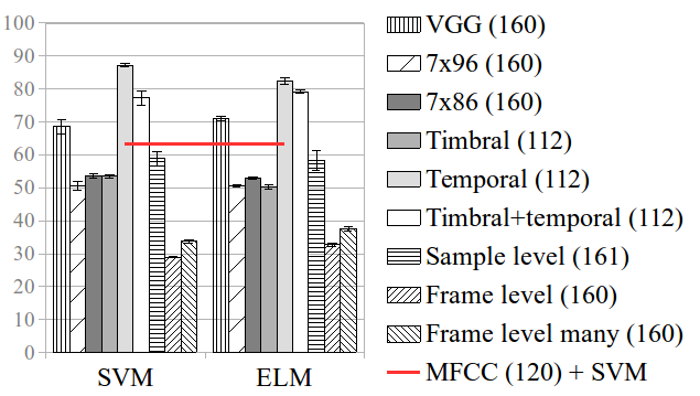
Figure 8: Accuracy (%) results for the Extended Ballroom dataset with random CNN feature vectors of length $\approx$ 120.

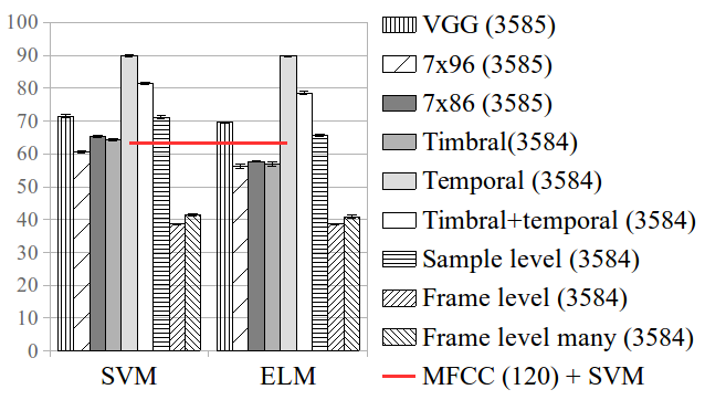
Figure 9: Accuracy (%) results for the Extended Ballroom dataset with random CNN feature vectors of length $\approx$ 3500

The sample-level waveform model always performs better than frame-level many-shapes (t-test: p-value$\ll$0.05). The two best performing spectrogram-based models are: temporal and timbral+temporal, but the temporal model performs better than timbral+temporal in all cases (t-test: p-value$\ll$0.05) – denoting that spectral cues can be a confounding factor for this dataset. Moreover, the 7x86 model performs better than 7x96 in all cases (t-test: p-value$<$0.05). The best (average) accuracy score is obtained using temporal models and SVMs ($\approx$3500): 89.82%. Note that the temporal model clearly outperforms the MFCCs baseline: 63.25%(t-test: p-value$\ll$0.05) and, interestingly, it performs slightly worse than a trained CNN: 93.7% [20]. This result confirms that the architectures (alone) introduce a strong prior which can significantly affect the performance of an audio model. Thus meaning that, besides learning, designing effective architectures might be key for resolving (music) audio tasks with deep learning. In line with that, note that the temporal architecture is designed considering musical domain knowledge – in this case: how tempo & rhythm are expressed in spectrograms. Hence, its good performance also validates the design strategy of using musically motivated architectures as a way to intuitively navigate through the network parameters space [36, 39, 38].

4.3 Urban Sounds 8K: acoustic event detection

For these experiments we do not use the temporal model (with 1D-CNNs of length 165, 128, 64, 32). Instead, we study the temporal+time model – where time follows the same design as temporal but with filters of length: 64, 32, 16, 8. This change is motivated by the fact that temporal cues in (natural) sounds are shorter and less important than temporal cues in music (i.e., rhythm or tempo).

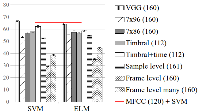
Figure 10: Accuracy (%) results for the Urban Sounds 8k dataset with random CNN feature vectors of length $\approx$ 120.

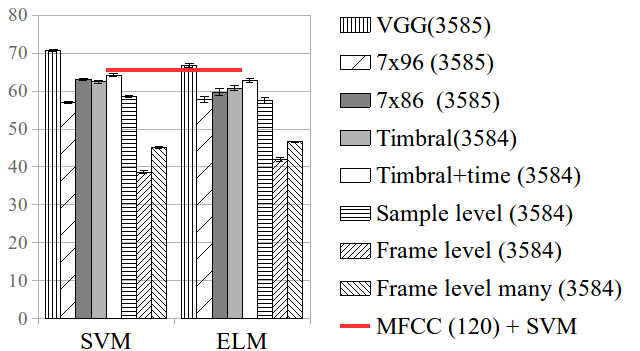
Figure 11: Accuracy (%) results for the Urban Sounds 8k dataset with random CNN feature vectors of length $\approx$ 3500

The sample-level waveform model always performs better than frame-level many-shapes (t-test: p-value$\ll$0.05). The two best performing spectrogram-based models are: VGG and timbral+time – but VGG performs better than timbral+time in all cases (t-test: p-value$\ll$0.05). Also, the 7x86 model performs better than 7x96 in all cases (t-test: p-value$<$0.075). The best (average) accuracy score is obtained using VGG and SVMs ($\approx$3500): 70.74% – outperforming the MFCCs baseline: 65.49%(t-test: p-value$<$0.05), and performing slightly worse than a trained CNN: 73%[28]. Finally, note that VGGs achieved remarkable results when recognizing genres and detecting acoustic events – tasks where timbre is an important cue. As a result: one could argue that VGGs are good at representing spectral features. Hence, these might be of utility for tasks where spectral cues are relevant.

5 CONCLUSIONS

This study builds on top of prior works showing that the (classification) performance delivered by random CNN features is correlated with the results of their end-to-end trained counterparts [43, 41]. We use this property to run a comprehensive evaluation of current deep architectures for (music) audio. Our method is as follows: first, we extract a feature vector from the embeddings of a randomly weighted CNN; and then, we input these features to a classifier – which can be an SVM or an ELM. Our goal is to compare the obtained classification accuracies when using different CNN architectures. The results we obtain are far from random, since: (i) randomly weighted CNNs are (in some cases) close to match the accuracies obtained by trained CNNs; and (ii) these are able to outperform MFCCs. This result denotes that the architectures alone are an important piece of the deep learning solution and therefore, searching for efficient architectures capable to encode the specificities of (music) audio signals might help advancing the state of our field. In line with that, we have shown that (musical) priors embedded in the structure of the model can facilitate capturing useful (temporal) cues for classifying rhythm/tempo classes. Besides, we show that for waveform front-ends: sample-level $\gg$ frame-level many-shapes $>$ frame-level – as noted in the (trained) literature [27, 53, 52]. The differential aspect of the sample-level front-end is that its representational power is constructed via hierarchically combining small-context representations, not by exploiting prior knowledge about waveforms. Further, we show that for spectrogram front-ends:7x96$<$7x86 – as shown in prior (trained) works [36, 31]. By allowing the filters to convolve through the frequency axis, the architecture itself facilitates capturing pitch-invariant timbral representations. Finally: timbral (+temporal/time) and VGG spectrogram front-ends achieve remarkable results for tasks where timbre is important – as previously noted in the (trained) literature [39]. Their respective advantages being that: (i) timbral (+temporal/time) architectures are single-layered front-ends which explicitly capture acoustically relevant receptive fields – which can be known via exploiting prior knowledge about the task; and (ii) VGG front-ends require no prior domain knowledge about the task for its design. Although our main conclusions are backed by additional results in the (trained) literature, we leave for future work consolidating those via doing a similar study considering trained models.

6 ACKNOWLEDGMENTS

This work was partially supported by the Maria de Maeztu Units of Excellence Programme (MDM-2015-0502) – and we are grateful for the GPUs donated by NVidia.

References

- [1] Julius Adebayo, Justin Gilmer, Ian Goodfellow, and Been Kim. Local explanation methods for deep neural networks lack sensitivity to parameter values. In International Conference on Learning Representations Workshop (ICLR), 2018.
- [2] Relja Arandjelovic and Andrew Zisserman. Look, listen and learn. In IEEE International Conference on Computer Vision (ICCV), pages 609–617. IEEE, 2017.
- [3] Judith C Brown. Calculation of a constant q spectral transform. The Journal of the Acoustical Society of America, 89(1):425–434, 1991.
- [4] Pedro Cano, Emilia Gómez, Fabien Gouyon, Perfecto Herrera, Markus Koppenberger, Beesuan Ong, Xavier Serra, Sebastian Streich, and Nicolas Wack. ISMIR 2004 audio description contest. Music Technology Group of the Universitat Pompeu Fabra, Technical Report, 2006.
- [5] Ning Chen and Shijun Wang. High-level music descriptor extraction algorithm based on combination of multi-channel cnns and lstm. In International Society for Music Information Retrieval Conference (ISMIR), 2017.
- [6] Keunwoo Choi, George Fazekas, and Mark Sandler. Automatic tagging using deep convolutional neural networks. International Society for Music Information Retrieval Conference (ISMIR), 2016.
- [7] Keunwoo Choi, György Fazekas, Mark Sandler, and Kyunghyun Cho. Transfer learning for music classification and regression tasks. International Society for Music Information Retrieval Conference (ISMIR), 2017.
- [8] Djork-Arné Clevert, Thomas Unterthiner, and Sepp Hochreiter. Fast and accurate deep network learning by exponential linear units (elus). arXiv preprint arXiv:1511.07289, 2015.
- [9] Sander Dieleman and Benjamin Schrauwen. End-to-end learning for music audio. In IEEE International Conference on Acoustics, Speech and Signal Processing (ICASSP), 2014.
- [10] Xavier Glorot, Antoine Bordes, and Yoshua Bengio. Deep sparse rectifier neural networks. In International Conference on Artificial Intelligence and Statistics, pages 315–323, 2011.
- [11] Rong Gong, Jordi Pons, and Xavier Serra. Audio to score matching by combining phonetic and duration information. International Society for Music Information Retrieval Conference (ISMIR), 2017.
- [12] Ian J Goodfellow, Jonathon Shlens, and Christian Szegedy. Explaining and harnessing adversarial examples. arXiv preprint arXiv:1412.6572, 2014.
- [13] Kun Han, Dong Yu, and Ivan Tashev. Speech emotion recognition using deep neural network and extreme learning machine. In Annual Conference of the International Speech Communication Association, 2014.
- [14] Kaiming He, Xiangyu Zhang, Shaoqing Ren, and Jian Sun. Delving deep into rectifiers: Surpassing human-level performance on imagenet classification. In IEEE International Conference on Computer Vision (ICCV), pages 1026–1034, 2015.
- [15] Kaiming He, Xiangyu Zhang, Shaoqing Ren, and Jian Sun. Deep residual learning for image recognition. In IEEE conference on Computer Vision and Pattern Recognition (CVPR), pages 770–778, 2016.
- [16] Georg Holzmann. Reservoir computing: A powerful black-box framework for nonlinear audio processing. In International Conference on Digital Audio Effect (DAFx), 2009.
- [17] Gao Huang, Zhuang Liu, Kilian Q Weinberger, and Laurens van der Maaten. Densely connected convolutional networks. In IEEE conference on Computer Vision and Pattern Recognition (CVPR), volume 1, page 3, 2017.
- [18] Guang-Bin Huang, Qin-Yu Zhu, and Chee-Kheong Siew. Extreme learning machine: theory and applications. Neurocomputing, 70(1-3):489–501, 2006.
- [19] Herbert Jaeger. The “echo state” approach to analysing and training recurrent neural networks-with an erratum note. German National Research Center for Information Technology, Technical Report, 148(34):13, 2001.
- [20] Yeonwoo Jeong, Keunwoo Choi, and Hosan Jeong. Dlr: Toward a deep learned rhythmic representation for music content analysis. arXiv preprint arXiv:1712.05119, 2017.
- [21] Heysem Kaya and Albert Ali Salah. Combining modality-specific extreme learning machines for emotion recognition in the wild. Journal on Multimodal User Interfaces, 10(2):139–149, 2016.
- [22] Corey Kereliuk, Bob L Sturm, and Jan Larsen. Deep learning and music adversaries. IEEE Transactions on Multimedia, 17(11):2059–2071, 2015.
- [23] Suisin Khoo, Zhihong Man, and Zhenwei Cao. Automatic han chinese folk song classification using extreme learning machines. In Australasian Joint Conference on Artificial Intelligence, pages 49–60. Springer, 2012.
- [24] Jaehun Kim, Julián Urbano, Cynthia Liem, and Alan Hanjalic. One deep music representation to rule them all?: A comparative analysis of different representation learning strategies. arXiv preprint arXiv:1802.04051, 2018.
- [25] Alex Krizhevsky, Ilya Sutskever, and Geoffrey E Hinton. Imagenet classification with deep convolutional neural networks. In Advances in Neural Information Processing Systems (NIPS), pages 1097–1105, 2012.
- [26] Honglak Lee, Peter Pham, Yan Largman, and Andrew Y Ng. Unsupervised feature learning for audio classification using convolutional deep belief networks. In Advances in Neural Information Processing Systems (NIPS), 2009.
- [27] Jongpil Lee, Jiyoung Park, Keunhyoung Luke Kim, and Juhan Nam. Sample-level deep convolutional neural networks for music auto-tagging using raw waveforms. Sound and Music Computing Conference (SMC), 2017.
- [28] Jongpil Lee, Jiyoung Park, Keunhyoung Luke Kim, and Juhan Nam. Samplecnn: End-to-end deep convolutional neural networks using very small filters for music classification. Applied Sciences, 8(1):150, 2018.
- [29] Qi-Jun Benedict Loh and Sabu Emmanuel. Elm for the classification of music genres. In International Conference on Control, Automation, Robotics and Vision, pages 1–6. IEEE, 2006.
- [30] Ugo Marchand and Geoffroy Peeters. Scale and shift invariant time/frequency representation using auditory statistics: Application to rhythm description. In International Workshop on Machine Learning for Signal Processing, pages 1–6. IEEE, 2016.
- [31] Sergio Oramas, Oriol Nieto, Francesco Barbieri, and Xavier Serra. Multi-label music genre classification from audio, text, and images using deep features. International Society for Music Information Retrieval Conference (ISMIR), 2017.
- [32] Yoh-Han Pao, Gwang-Hoon Park, and Dejan J Sobajic. Learning and generalization characteristics of the random vector functional-link net. Neurocomputing, 6(2):163–180, 1994.
- [33] F. Pedregosa, G. Varoquaux, A. Gramfort, V. Michel, B. Thirion, O. Grisel, M. Blondel, P. Prettenhofer, R. Weiss, V. Dubourg, J. Vanderplas, A. Passos, D. Cournapeau, M. Brucher, M. Perrot, and E. Duchesnay. Scikit-learn: Machine learning in Python. Journal of Machine Learning Research, 12:2825–2830, 2011.
- [34] Huy Phan, Lars Hertel, Marco Maass, and Alfred Mertins. Robust audio event recognition with 1-max pooling convolutional neural networks. arXiv preprint arXiv:1604.06338, 2016.
- [35] Jordi Pons, Rong Gong, and Xavier Serra. Score-informed syllable segmentation for a cappella singing voice with convolutional neural networks. International Society for Music Information Retrieval Conference (ISMIR), 2017.
- [36] Jordi Pons, Thomas Lidy, and Xavier Serra. Experimenting with musically motivated convolutional neural networks. In International Workshop on Content-Based Multimedia Indexing (CBMI), pages 1–6. IEEE, 2016.
- [37] Jordi Pons, Oriol Nieto, Matthew Prockup, Erik M Schmidt, Andreas F Ehmann, and Xavier Serra. End-to-end learning for music audio tagging at scale. Workshop on Machine Learning for Audio Signal Processing (ML4Audio) at NIPS, 2017.
- [38] Jordi Pons and Xavier Serra. Designing efficient architectures for modeling temporal features with convolutional neural networks. In IEEE International Conference on Acoustics, Speech and Signal Processing (ICASSP), 2017.
- [39] Jordi Pons, Olga Slizovskaia, Rong Gong, Emilia Gómez, and Xavier Serra. Timbre analysis of music audio signals with convolutional neural networks. European Signal Processing Conference (EUSIPCO), 2017.
- [40] Dario Rethage, Jordi Pons, and Xavier Serra. A Wavenet for speech denoising. IEEE International Conference on Acoustics, Speech and Signal Processing (ICASSP), 2018.
- [41] Amir Rosenfeld and John K Tsotsos. Intriguing properties of randomly weighted networks: Generalizing while learning next to nothing. arXiv preprint arXiv:1802.00844, 2018.
- [42] J. Salamon, C. Jacoby, and J. P. Bello. A dataset and taxonomy for urban sound research. In ACM International Conference on Multimedia, Orlando, FL, USA, Nov. 2014.
- [43] Andrew M Saxe, Pang Wei Koh, Zhenghao Chen, Maneesh Bhand, Bipin Suresh, and Andrew Y Ng. On random weights and unsupervised feature learning. In International Conference on Machine Learning (ICML), pages 1089–1096, 2011.
- [44] Simone Scardapane, Danilo Comminiello, Michele Scarpiniti, and Aurelio Uncini. Music classification using extreme learning machines. In International Symposium on Image and Signal Processing and Analysis (ISPA), pages 377–381. IEEE, 2013.
- [45] Simone Scardapane and Aurelio Uncini. Semi-supervised echo state networks for audio classification. Cognitive Computation, 9(1):125–135, 2017.
- [46] Jan Schluter and Sebastian Bock. Improved musical onset detection with convolutional neural networks. In IEEE International Conference on Acoustics, Speech and Signal Processing (ICASSP), 2014.
- [47] Wouter F Schmidt, Martin A Kraaijveld, and Robert PW Duin. Feedforward neural networks with random weights. In International Conference on Pattern Recognition, pages 1–4. IEEE, 1992.
- [48] Karen Simonyan and Andrew Zisserman. Very deep convolutional networks for large-scale image recognition. arXiv preprint arXiv:1409.1556, 2014.
- [49] Christian Szegedy, Wojciech Zaremba, Ilya Sutskever, Joan Bruna, Dumitru Erhan, Ian Goodfellow, and Rob Fergus. Intriguing properties of neural networks. arXiv preprint arXiv:1312.6199, 2013.
- [50] George Tzanetakis and Perry Cook. Musical genre classification of audio signals. IEEE Transactions on speech and audio processing, 10(5):293–302, 2002.
- [51] Dmitry Ulyanov, Andrea Vedaldi, and Victor Lempitsky. Deep image prior. arXiv preprint arXiv:1711.10925, 2017.
- [52] Aaron Van Den Oord, Sander Dieleman, Heiga Zen, Karen Simonyan, Oriol Vinyals, Alex Graves, Nal Kalchbrenner, Andrew Senior, and Koray Kavukcuoglu. Wavenet: A generative model for raw audio. arXiv preprint arXiv:1609.03499, 2016.
- [53] Zhenyao Zhu, Jesse H Engel, and Awni Hannun. Learning multiscale features directly from waveforms. arXiv preprint arXiv:1603.09509, 2016.