\Type\Title

Robust Log-Optimal Strategy with Reinforcement Learning

\Author

YiFeng Guo  XingYu Fu  YuYan Shi  MingWen Liu

\Author

Sun Yat-sen University

\Abstract

We proposed a new Portfolio Management method termed as Robust Log-Optimal Strategy (RLOS), which ameliorates the General Log-Optimal Strategy (GLOS) by approximating the traditional objective function with quadratic Taylor expansion. It avoids GLOS’s complex CDF estimation process, hence resists the ”Butterfly Effect” caused by estimation error. Besides, RLOS retains GLOS’s profitability and the optimization problem involved in RLOS is computationally far more practical compared to GLOS. Further, we combine RLOS with Reinforcement Learning (RL) and propose the so-called Robust Log-Optimal Strategy with Reinforcement Learning (RLOSRL), where the RL agent receives the analyzed results from RLOS and observes the trading environment to make comprehensive investment decisions. The RLOSRL’s performance is compared to some traditional strategies on several back tests, where we randomly choose a selection of constituent stocks of the CSI300 index as assets under management and the test results validate its profitability and stability.
Keywords:Portfolio Management; Mathematical Finance; Artificial Intelligence; Information theory; Log-Optimal Strategy; Robustness Analysis; Reinforcement Learning; Deep Learning; Convolutional Neural Network.

1 Introduction

Portfolio Management (PM), aiming to balance risk and return optimally, sequentially allocating an amount of wealth to a collection of assets in some consecutive trading periods based on investors’ return-risk profile [9], is a crucial problem in both theoretical and practical aspects of finance. There are mainly four types of PM strategies [11] proposed from both industry and academia, i.e. Follow-the-Winner, which allocates wealth to the best performed asset; Follow-the-Loser, which allocates wealth to the worst performed asset; Pattern-Matching, which predicts the distribution of price fluctuation of the next trading period based on historical data and chooses the optimal portfolio according to the prediction; Meta-Learning, which combines several different PM strategies to form a better-performed Ensembled investment policy; In our work, we focus on the latter two types, where we ensemble two algorithms from Pattern-Matching category, i.e. Log-Optimal based Strategy and Reinforcement Learning based Strategy, to form our final PM policy.

The General Log-Optimal Strategy (GLOS), originated from information theory [1], attempting to maximize the expectation of the logarithmic rate of return by choosing optimal portfolio weight, is a natural and one of the most renowned PM methods, where many exciting results emerge [10,12,13]. In our work, we will prove rigorously that GLOS is endowed with many elegant characteristics, i.e. Information-Benefit, Greed, and Long-Term Superiority, which justifies its importance. While in practice, the complicated estimation of Cumulative Distribution Function (CDF) and high computational complexity of GLOS make it hard to employ in finance industry, and therefore we propose the so-called Robust Log-Optimal Strategy (RLOS) which avoids GLOS’s complex CDF estimation process, hence resists the ”Butterfly Effect” caused by estimation error. Besides, RLOS retains GLOS’s profitability and the optimization problem involved in RLOS is computationally far more practical compared to GLOS.

Reinforcement Learning (RL) has witnessed tremendous success in various agent-environment interaction tasks [2,3,4] and it is believed to a possible avenue to the General Artificial Intelligence, where many large companies (e.g. Google DeepMind; Facebook; Baidu etc.) are leading its pioneer research. It is also natural to apply the RL technique to the PM scenario [14,15], where the agent gets reward if its investment decision increases the logarithmic rate of return and gets punishment if it decreases. In our work, we train a RL agent managing a selection of assets on the highly noisy finance environment [5], who receives the analyzed results from RLOS and observes the trading environment using deep Convolutional Neural Network (CNN) simultaneously. The loss function of the RL algorithm, which is composed of reward and penalty, is designed to guide the virtual portfolio manager to trade in a maximizing-profit way. We term the ensemble of RLOS and RL as Robust Log-Optimal Strategy with Reinforcement Learning (RLOSRL).

Our strategies are back-tested on several random selections(Bootstrapping) of constituent stocks of CSI300 index competing with Naïve-Average, Follow-the-Loser, and Follow-the-Winner. RLOSRL and RLOSRL outperforms all these three strategies in all of the back tests, validating the profitability and stability of our algorithm. Further, we can see from the back tests that the trading behaviors of RLOS and RLOSRL are similar to some extent, while RLOSRL defeats RLOS in all back tests, demonstrating the advances of RL.111The implementation can be viewed at https://github.com/fxy96/Robust-Log-Optimal-Strategy-with-Reinforcement-Learning

2 General Log-Optimal Strategy

PM is one of the most common investment methods by managing a collection of assets to optimize a certain objective function. The objective function is often the trade-off between expected risk and expected return for a long-term investment horizon, while in the context of GLOS, the objective function is the expectation of logarithmic rate of return. In this section, we will first define the GLOS formally and then we will study three important characteristics of the strategy, i.e. Information-Benefit, Greed and Long-Term Superiority.

2.1 Definition of GLOS

Say we have d𝑑d assets under management in a single trading period. Let X=(X1,X2,,Xd)TXsuperscriptsubscript𝑋1subscript𝑋2subscript𝑋𝑑𝑇\textbf{X}=(X_{1},X_{2},...,X_{d})^{T} represent the asset price fluctuation vector in a single trading period and b=(b1,b2,,bd)Tbsuperscriptsubscript𝑏1subscript𝑏2subscript𝑏𝑑𝑇\textbf{b}=(b_{1},b_{2},...,b_{d})^{T} denote the portfolio weight vector that we set at the start of the trading period. For X, each Xisubscript𝑋𝑖X_{i} in X is defined as the ratio of the closing price to the opening price of the ithsubscript𝑖𝑡i_{th} asset over the trading period and X can be deemed as a random vector where we use F to represent its CDF.For b, each bisubscript𝑏𝑖b_{i} in b is defined as proportion of the ithsubscript𝑖𝑡i_{th} asset’s investment to the total investment and choosing the optimal b at the start of the trading period is the mission of portfolio manager.

In the context of GLOS, the portfolio manager tries to maximize the expected logarithmic rate of return, i.e. choosing bXsuperscriptsubscript𝑏𝑋b_{X}^{*} satisfying the following equation:

𝐛𝐗argmaxbBrX(b)superscriptsubscript𝐛𝐗subscriptb𝐵subscript𝑟Xb\mathbf{b_{X}^{*}}\in\mathop{\arg\max}_{\textbf{b}\in B}r_{\textbf{X}}(\textbf{b}) (1)

where rX(b)=Elog(bTX)=log(bTx)𝑑F(x)subscript𝑟Xb𝐸𝑙𝑜𝑔superscriptb𝑇X𝑙𝑜𝑔superscriptb𝑇xdifferential-d𝐹xr_{\textbf{X}}(\textbf{b})=Elog(\textbf{b}^{T}\textbf{X})=\int{log(\textbf{b}^{T}\textbf{x})dF(\textbf{x})} is the expected logarithmic rate of return and B𝐵B is the constrain exerted on b.

The above analysis is set on a single trading period, while in practice, we usually trade on consecutive trading periods, which results in a sequence of {Xi}i=1nsuperscriptsubscriptsubscriptX𝑖𝑖1𝑛\{\textbf{X}_{i}\}_{i=1}^{n}. If {Xi}i=1nsuperscriptsubscriptsubscriptX𝑖𝑖1𝑛\{\textbf{X}_{i}\}_{i=1}^{n} is independent and identically distributed (i.i.d). over different trading periods, then optimal portfolio weight vector which maximizes the expectation of the logarithmic rate of return is the same for every trading period since the objective function is the same and no interdependence of different periods. While in general case, the i.i.d assumption does not hold.

2.2 Characteristics of GLOS

The reason why we study the GLOS is the elegant mathematical foundations behind it, i.e. Information-Benefit, Greed, and Long-Term Superiority.

2.2.1 Information-Benefit

Market Information influences the trading environment directly in a way that can be detected by the GLOS. We call this property as Information-Benefit.

Say we now trade on a sequence of consecutive trading periods. When new market information arrives at each trading period, the i.i.d assumption of the distribution of {Xi}i=1nsuperscriptsubscriptsubscriptX𝑖𝑖1𝑛\{\textbf{X}_{i}\}_{i=1}^{n} will be violated and therefore we can’t just maintain a common portfolio weight vector bXsuperscriptsubscript𝑏𝑋b_{X}^{*} for every trading period. While the information also brings information benefit, i.e. it will increase the expectation of the optimal logarithmic rate of return which will be illustrated below.

Denote the information by Y𝑌Y and the conditional distribution of X given Y=y𝑌𝑦Y=y by F(X|Y=y)𝐹conditionalX𝑌𝑦F(\textbf{X}|Y=y) at each trading period. Let bX|YTsuperscriptsubscriptbconditionalX𝑌𝑇\textbf{b}_{\textbf{X}|Y}^{T*} be the optimal portfolio weight vector such that:

bX|YTsuperscriptsubscriptbconditionalX𝑌𝑇\displaystyle\textbf{b}_{\textbf{X}|Y}^{T*} argmaxbBrX|Y(b)absentsubscriptb𝐵subscript𝑟conditionalX𝑌b\displaystyle\in\mathop{\arg\max}_{\textbf{b}\in B}r_{\textbf{X}|Y}(\textbf{b}) (2)
=argmaxbBlog(bTx)𝑑F(x|Y=y)absentsubscriptb𝐵𝑙𝑜𝑔superscriptb𝑇xdifferential-d𝐹conditionalx𝑌𝑦\displaystyle=\mathop{\arg\max}_{\textbf{b}\in B}\int{log(\textbf{b}^{T}\textbf{x})dF(\textbf{x}|Y=y})

The increment of expected logarithmic rate of return is defined as:

ΔVY=rX|Y(bX|YTx)rX|Y(bXTx)Δsubscript𝑉𝑌subscript𝑟conditionalX𝑌superscriptsubscriptbconditionalX𝑌𝑇xsubscript𝑟conditionalX𝑌superscriptsubscriptbX𝑇x\Delta V_{Y}=r_{\textbf{X}|Y}(\textbf{b}_{\textbf{X}|Y}^{T*}\textbf{x})-r_{\textbf{X}|Y}(\textbf{b}_{\textbf{X}}^{T*}\textbf{x}) (3)

ΔVYΔsubscript𝑉𝑌\Delta V_{Y} satisfies some elegant mathematical properties which give it some reasonable constrains.

Theorem 2.1.

Suppose ΔV=E(ΔVY)Δ𝑉𝐸Δsubscript𝑉𝑌\Delta V=E(\Delta V_{Y}). ΔVYΔsubscript𝑉𝑌\Delta V_{Y} and ΔVΔ𝑉\Delta V satisfies:

  1. 1)

    ΔVY0Δsubscript𝑉𝑌0\Delta V_{Y}\geq 0

  2. 2)

    ΔVYfX|Y=y(x)logfX|Y=y(x)f(x)𝑑xΔsubscript𝑉𝑌subscript𝑓conditionalX𝑌𝑦x𝑙𝑜𝑔subscript𝑓conditionalX𝑌𝑦x𝑓xdifferential-dx\Delta V_{Y}\leq\int{f_{\textbf{X}|Y=y}(\textbf{x})log\frac{f_{\textbf{X}|Y=y}(\textbf{x})}{f(\textbf{x})}d\textbf{x}}

  3. 3)

    ΔVh(x,y)logh(x,y)f(x)g(y)𝑑x𝑑yΔ𝑉double-integralx𝑦𝑙𝑜𝑔x𝑦𝑓x𝑔𝑦differential-dxdifferential-d𝑦\Delta V\leq\iint{h(\textbf{x},y)log\frac{h(\textbf{x},y)}{f(\textbf{x})g(y)}d\textbf{x}dy}

where f,g𝑓𝑔f,g are the marginalized density functions for X and Y𝑌Y respectively and hh is the joint density function of X and Y𝑌Y.
See the proof in the appendix.

Note that ΔVYΔsubscript𝑉𝑌\Delta V_{Y} and ΔVΔ𝑉\Delta V are controlled by some upper bounds, which means the increment of expected logarithmic rate of return brought by information benefit is not in an unreasonable scale.

Further, note that ΔVΔ𝑉\Delta V has an upper bound h(x,y)logh(x,y)f(x)g(y)𝑑x𝑑ydouble-integralx𝑦𝑙𝑜𝑔x𝑦𝑓x𝑔𝑦differential-dxdifferential-d𝑦\iint{h(\textbf{x},y)log\frac{h(\textbf{x},y)}{f(\textbf{x})g(y)}d\textbf{x}dy}, which is the mutual information between X and Y𝑌Y, a concept frequently studied in information theory [1]. When X and Y𝑌Y are independent, we see that ΔV=0Δ𝑉0\Delta V=0 (Independence implies that the joint density function equals to the product of marginalized density functions), which indicates that no information has been detected by the trading strategy. When X is completely determined by Y𝑌Y, this upper bound is exactly the entropy of the information Y𝑌Y, another important concept studied in information theory [1]. Further explanation of the upper bound may be intriguing but is out of the scope of this paper and we leave the exploration of this avenue for future research.

2.2.2 Greed and Long-Term Superiority

Say we trade on some consecutive trading periods. When {Xi}i=1nsuperscriptsubscriptsubscriptX𝑖𝑖1𝑛\{\textbf{X}_{i}\}_{i=1}^{n} is i.i.d, the GLOS maintains a certain fixed portfolio weight vector bXsuperscriptsubscript𝑏𝑋b_{X}^{*} for all trading periods at the start. While, due to the market information which we have discussed in section 2.2.1, the i.i.d. assumption does not hold. Fortunately, the i.i.d. assumption is not necessary. The GLOS can make greedy investment decision for every trading period, i.e. only focusing on maximizing the expected logarithmic rate of return for each single trading period, while the strategy is still superior to other strategies asymptotically in the view of final gross wealth.

Denote the final gross wealth at the end of the nthsubscript𝑛𝑡n_{th} trading period with a sequence of portfolio weight vector {bi}i=1nsuperscriptsubscriptsubscriptb𝑖𝑖1𝑛\{\textbf{b}_{i}\}_{i=1}^{n} by Sn=S0Πi=1nbiTXisubscript𝑆𝑛subscript𝑆0superscriptsubscriptΠ𝑖1𝑛superscriptsubscriptb𝑖𝑇subscriptX𝑖S_{n}=S_{0}\Pi_{i=1}^{n}\textbf{b}_{i}^{T}\textbf{X}_{i} and the final gross wealth using the GLOS Sn=S0Πi=1nbiTXisuperscriptsubscript𝑆𝑛subscript𝑆0superscriptsubscriptΠ𝑖1𝑛superscriptsubscriptb𝑖absent𝑇subscriptX𝑖S_{n}^{*}=S_{0}\Pi_{i=1}^{n}\textbf{b}_{i}^{*T}\textbf{X}_{i}. Next theorem indicates the superiority of the General Log-Optimal Strategy over other PM strategies.

Theorem 2.2.

Snsuperscriptsubscript𝑆𝑛S_{n}^{*} is asymptotically superior to Snsubscript𝑆𝑛S_{n} with probability 1.
Proof: See the proof in the appendix.

3 Robust Log-Optimal Strategy

There are several disadvantages to implement the GLOS in finance industry. In GLOS, we assume the CDF F(x)𝐹xF(\textbf{x}) of price fluctuation vector X is given, while in practice, it’s impossible for portfolio manager to know F(x)𝐹xF(\textbf{x}) in advance. To implement GLOS, they need to estimate F(x)𝐹xF(\textbf{x}) from historical data with certain assumptions, where the estimation error and the improper assumptions may cause the so-called ”Butterfly Effect”. Besides, even if we have known F(x)𝐹xF(\textbf{x}) already, it is computationally expensive to optimize the objective function log(bTx)𝑑F(x)𝑙𝑜𝑔superscriptb𝑇xdifferential-d𝐹x\int{log(\textbf{b}^{T}\textbf{x})dF(\textbf{x})} of GLOS since the high dimensionality of X and b and the logarithmic operation in the expression.

Therefore, we propose RLOS, where we don’t estimate F(x)𝐹xF(\textbf{x}) and maximize log(bTx)𝑑F(x)𝑙𝑜𝑔superscriptb𝑇xdifferential-d𝐹x\int{log(\textbf{b}^{T}\textbf{x})dF(\textbf{x})} directly. In RLOS, we introduce a new objective function called the Allocation Utility, which is a quadratic Taylor approximation to the expectation of the logarithmic rate of return, and it is so simple that only involves the expectation and covariance of X. Indeed, it can be viewed as the trade-off between the logarithmic return and its squared coefficient of variation.

RLOS is computationally effective compared to GLOS, and it is robust in the sense that the upper bound of Allocation Utility deviation can be controlled by the L1subscript𝐿1L_{1}-norm of portfolio weight vector and Lsubscript𝐿L_{\infty}-norm of the bias of covariance matrix estimator.

3.1 Objective function of RLOS (Allocation Utility)

The GLOS has (1). However, the optimization problem relies on the distribution function of X ,which is hard to know in practice.

Supposing X’s expectation is 𝝁𝝁\boldsymbol{\mu} and its covariance matrix is 𝚺𝚺\mathbf{\Sigma} , in RLOS, we adopt quadratic Taylor expansion to approximate Elog(bTX)𝐸𝑙𝑜𝑔superscriptb𝑇XElog(\textbf{b}^{T}\textbf{X}).

Thus, we define the Allocation Utility, which is the objective function of RLOS, as:

M(𝐛,𝝁,𝚺)=log(𝐛T𝝁)12(𝐛T𝝁)2𝐛T𝚺𝐛𝑀𝐛𝝁𝚺𝑙𝑜𝑔superscript𝐛𝑇𝝁12superscriptsuperscript𝐛𝑇𝝁2superscript𝐛𝑇𝚺𝐛M(\mathbf{b},\boldsymbol{\mu},\boldsymbol{\Sigma})=log(\mathbf{b}^{T}\boldsymbol{\mu})-\frac{1}{2(\mathbf{b}^{T}\boldsymbol{\mu})^{2}}\mathbf{b}^{T}\mathbf{\Sigma}\mathbf{b} (4)
Seethedetailsofcomputationintheappendix.𝑆𝑒𝑒𝑡𝑒𝑑𝑒𝑡𝑎𝑖𝑙𝑠𝑜𝑓𝑐𝑜𝑚𝑝𝑢𝑡𝑎𝑡𝑖𝑜𝑛𝑖𝑛𝑡𝑒𝑎𝑝𝑝𝑒𝑛𝑑𝑖𝑥See\ the\ details\ of\ computation\ in\ the\ appendix.

By maximizing M(𝐛,𝝁,𝚺)𝑀𝐛𝝁𝚺M(\mathbf{b},\boldsymbol{\mu},\boldsymbol{\Sigma}), which is the mission of RLOS, we can estimate the solution to GLOS in a robust manner. Note that M(𝐛,𝝁,𝚺)𝑀𝐛𝝁𝚺M(\mathbf{b},\boldsymbol{\mu},\boldsymbol{\Sigma}) doesn’t involve the distribution function of X and the parameters to be estimated are only the expectation and covariance of X, which is far more practical than the objective function in GLOS, where the estimation of F(x)𝐹xF(\textbf{x}) is required.

Besides, M(𝐛,𝝁,𝚺)𝑀𝐛𝝁𝚺M(\mathbf{b},\boldsymbol{\mu},\boldsymbol{\Sigma}) can be deemed as a trade-off between the logarithmic return and its squared coefficient of variation, which somehow coincides with Markowitz’s ”expected returns – variance of returns” rule [9].

3.2 Optimal portfolio weight vector for RLOS

Consider the optimization problem in RLOS:

𝐛𝐨𝐩𝐭argmaxM(𝐛,𝝁,𝚺),s.t.𝐛Bformulae-sequencesuperscript𝐛𝐨𝐩𝐭𝑀𝐛𝝁𝚺𝑠𝑡𝐛𝐵\mathbf{b^{opt}}\in\mathop{\arg\max}M(\mathbf{b},\boldsymbol{\mu},\boldsymbol{\Sigma}),s.t.\mathbf{b}\in B

𝐛𝐨𝐩𝐭superscript𝐛𝐨𝐩𝐭\mathbf{b^{opt}} can be solved analytically for some natural constrain region 𝐵𝐵𝐵 if 𝝁,𝚺𝝁𝚺\boldsymbol{\mu},\boldsymbol{\Sigma} are given. For example, we take B={𝐛|𝐛T𝐞=1,𝐛T𝝁c,where𝐞=(1,1,,1)T}𝐵conditional-set𝐛formulae-sequencesuperscript𝐛𝑇𝐞1formulae-sequencesuperscript𝐛𝑇𝝁𝑐𝑤𝑒𝑟𝑒𝐞superscript111𝑇B=\{\mathbf{b}|\mathbf{b}^{T}\mathbf{e}=1,\mathbf{b}^{T}\boldsymbol{\mu}\geq c,where\ \mathbf{e}=(1,1,...,1)^{T}\}. The first constraint follows from the definition of portfolio weight vector and the second constraint accounts for the minimal expected rate of return. We apply Karush-Kuhn-Tucker condition to solve this optimization problem. We provide the computation in the appendix.

From the optimazition procedure, we can find that 𝐛𝐨𝐩𝐭superscript𝐛𝐨𝐩𝐭\mathbf{b^{opt}} depends on the value of 𝝁𝝁\boldsymbol{\mu} and 𝚺𝚺\boldsymbol{\Sigma} . If the estimation of 𝝁𝝁\boldsymbol{\mu},𝚺𝚺\boldsymbol{\Sigma} deviates from their true values, it may lead to deviation of estimation of optimal portfolio weight, which may result in the so-called ”Butterfly Effect”. Thus, we need to control our estimation process to reduce estimation deviation. In the next section, we will prove that the RLOS is robust which provides tolerance against reasonable estimation error.

3.3 Robustness Analysis of RLOS

Suppose that 𝐛^𝐨𝐩𝐭superscript^𝐛𝐨𝐩𝐭\mathbf{\hat{b}^{opt}} is the optimal portfolio weight vector estimator by replacing 𝝁𝝁\boldsymbol{\mu} and 𝚺𝚺\boldsymbol{\Sigma} with their estimators: 𝝁^^𝝁\hat{\boldsymbol{\mu}} and 𝚺^^𝚺\hat{\boldsymbol{\Sigma}}, in the optimization procedure. The estimation error of 𝝁^^𝝁\hat{\boldsymbol{\mu}} and 𝚺^^𝚺\hat{\boldsymbol{\Sigma}} may cause the so-called ”Butterfly Effect”. Hence, we need to study the robustness of RLOS.

We first give two reasonable assumptions here:

  1. 1)

    Suppose E(𝝁^)=𝝁𝐸^𝝁𝝁E(\hat{\boldsymbol{\mu}})=\boldsymbol{\mu}, i.e. 𝝁^^𝝁\hat{\boldsymbol{\mu}} is 𝝁𝝁\boldsymbol{\mu}’s unbiased estimation.

  2. 2)

    Let the entry in the ithsubscript𝑖𝑡i_{th} row and jthsubscript𝑗𝑡j_{th} column of 𝚺𝚺^𝚺^𝚺\boldsymbol{\Sigma}-\hat{\boldsymbol{\Sigma}} be σijsubscript𝜎𝑖𝑗\sigma_{ij}. We assume that maxiΣj=1n|σij|Msubscript𝑖superscriptsubscriptΣ𝑗1𝑛subscript𝜎𝑖𝑗𝑀\max\limits_{i}\Sigma_{j=1}^{n}|\sigma_{ij}|\leq M, where M𝑀M is a positive constant.

From 1), we know E(𝐛^𝐨𝐩𝐭T𝝁^)=𝐛^𝐨𝐩𝐭T𝝁𝐸superscript^𝐛superscript𝐨𝐩𝐭𝑇bold-^𝝁superscript^𝐛superscript𝐨𝐩𝐭𝑇𝝁E(\mathbf{\hat{b}}^{\mathbf{opt}^{T}}\boldsymbol{\hat{\mu}})=\mathbf{\hat{b}}^{\mathbf{opt}^{T}}\boldsymbol{\mu}. By Law of Large Number, ϵ>0for-allitalic-ϵ0\forall\epsilon>0 when sample size n𝑛n\to\infty, we have P(|𝐛^𝐨𝐩𝐭T𝝁^𝐛^𝐨𝐩𝐭T𝝁|>ϵ)0𝑃superscript^𝐛superscript𝐨𝐩𝐭𝑇bold-^𝝁superscript^𝐛superscript𝐨𝐩𝐭𝑇𝝁italic-ϵ0P(|\mathbf{\hat{b}}^{\mathbf{opt}^{T}}\boldsymbol{\hat{\mu}}-\mathbf{\hat{b}}^{\mathbf{opt}^{T}}\boldsymbol{\mu}|>\epsilon)\to 0. ϵ>0for-allitalic-ϵ0\forall\epsilon>0, n0N+subscript𝑛0subscript𝑁\exists n_{0}\in N_{+} such that 𝐛^^𝐛\mathbf{\hat{b}} satisfies |𝐛^𝐨𝐩𝐭T𝝁^𝐛^𝐨𝐩𝐭T𝝁|ϵsuperscript^𝐛superscript𝐨𝐩𝐭𝑇bold-^𝝁superscript^𝐛superscript𝐨𝐩𝐭𝑇𝝁italic-ϵ|\mathbf{\hat{b}}^{\mathbf{opt}^{T}}\boldsymbol{\hat{\mu}}-\mathbf{\hat{b}}^{\mathbf{opt}^{T}}\boldsymbol{\mu}|\leq\epsilon when sample size is more than n0subscript𝑛0n_{0}. Similar analysis with 2) so we don’t repeat it here.

Based on the above two assumptions, we now study deviation between M(𝐛^𝐨𝐩𝐭,,𝝁^,𝚺^)M(\mathbf{\hat{b}^{opt}},,\boldsymbol{\hat{\mu}},\boldsymbol{\hat{\Sigma}}) and M(𝐛^𝐨𝐩𝐭,𝝁,𝚺)𝑀superscript^𝐛𝐨𝐩𝐭𝝁𝚺M(\mathbf{\hat{b}^{opt}},\boldsymbol{\mu},\boldsymbol{\Sigma}), which reflects the robustness of RLOS.

Theorem 3.1.

Suppose 𝐛T𝛍csuperscript𝐛𝑇𝛍𝑐\mathbf{b}^{T}\boldsymbol{\mu}\geq c and satisfying the assumptions above, the bias of the RLOS following the estimation has an upper bound.

|M(𝐛^𝐨𝐩𝐭,𝝁^,𝚺^)M(𝐛^𝐨𝐩𝐭,𝝁,𝚺)|𝑀superscript^𝐛𝐨𝐩𝐭bold-^𝝁bold-^𝚺𝑀superscript^𝐛𝐨𝐩𝐭𝝁𝚺\displaystyle|M(\mathbf{\hat{b}^{opt}},\boldsymbol{\hat{\mu}},\boldsymbol{\hat{\Sigma}})-M(\mathbf{\hat{b}^{opt}},\boldsymbol{\mu},\boldsymbol{\Sigma})| (5)
\displaystyle\leq 12c2(i=1n|b^i|)2maxiΣj=1n|σij|12superscript𝑐2superscriptsuperscriptsubscript𝑖1𝑛subscript^𝑏𝑖2subscript𝑖superscriptsubscriptΣ𝑗1𝑛subscript𝜎𝑖𝑗\displaystyle\frac{1}{2c^{2}}(\sum_{i=1}^{n}|\hat{b}_{i}|)^{2}\max\limits_{i}\Sigma_{j=1}^{n}|\sigma_{ij}|

Proof: See the proof in the appendix.

Thus, if we choose a suitable constant c0>0subscript𝑐00c_{0}>0 and restrict i=1n|b^i|c0superscriptsubscript𝑖1𝑛subscript^𝑏𝑖subscript𝑐0\sum_{i=1}^{n}|\hat{b}_{i}|\leq c_{0}, we can ensure that the estimation error is controlled. Hence, to achieve a robust optimization result and make |M(𝐛^𝐨𝐩𝐭,𝝁^,𝚺^)M(𝐛^𝐨𝐩𝐭,𝝁,𝚺)|𝑀superscript^𝐛𝐨𝐩𝐭bold-^𝝁bold-^𝚺𝑀superscript^𝐛𝐨𝐩𝐭𝝁𝚺|M(\mathbf{\hat{b}^{opt}},\boldsymbol{\hat{\mu}},\boldsymbol{\hat{\Sigma}})-M(\mathbf{\hat{b}^{opt}},\boldsymbol{\mu},\boldsymbol{\Sigma})| controlled by an upper bound, we add an extra i=1n|b^i|c0superscriptsubscript𝑖1𝑛subscript^𝑏𝑖subscript𝑐0\sum_{i=1}^{n}|\hat{b}_{i}|\leq c_{0} constraint in the optimization procedure. We can explain the parameter c0subscript𝑐0c_{0} financially, which is larger than 1 if we allow short-selling and equals to 1 if short-selling is forbidden.

3.4 Implementation of RLOS

Say we now trade on the kthsubscript𝑘𝑡k_{th} trading period, to implement RLOS, the portfolio manager need to estimate the parameters involved in the objective function:

M(𝐛,𝝁,𝚺)=log(𝐛T𝝁)12(𝐛T𝝁)2𝐛T𝚺𝐛𝑀𝐛𝝁𝚺𝑙𝑜𝑔superscript𝐛𝑇𝝁12superscriptsuperscript𝐛𝑇𝝁2superscript𝐛𝑇𝚺𝐛M(\mathbf{b},\boldsymbol{\mu},\boldsymbol{\Sigma})=log(\mathbf{b}^{T}\boldsymbol{\mu})-\frac{1}{2(\mathbf{b}^{T}\boldsymbol{\mu})^{2}}\mathbf{b}^{T}\mathbf{\Sigma}\mathbf{b} (4)

i.e. we need to estimate the expectation 𝝁𝝁\boldsymbol{\mu} and the covariance matrix 𝚺𝚺\boldsymbol{\Sigma} of 𝐗𝐤subscript𝐗𝐤\mathbf{X_{k}} in the kthsubscript𝑘𝑡k_{th} trading period.

To estimate the parameters, our PM strategy selects a collection of trading periods that are similar to the kthsubscript𝑘𝑡k_{th} trading period and we then calculate 𝝁^^𝝁\hat{\boldsymbol{\mu}} and 𝚺^^𝚺\hat{\boldsymbol{\Sigma}} based on the collection, which is the methodology of Pattern-Matching[11]. The problem remains to be solved is how to define similarity between trading periods, where we define it as the Pearson Correlation between market backgrounds of trading periods. We now go specifically into the implementation.

3.4.1 Definition of Market Backgrounds

Consider trading background of the ithsubscript𝑖𝑡i_{th} trading period, we define it as the price fluctuation matrix reflecting the market situation from (in)thsubscript𝑖𝑛𝑡(i-n)_{th} to (i1)thsubscript𝑖1𝑡(i-1)_{th} trading periods. Formally, we write it as:

Background(ith,n)=[x1,(in)x1,(i1)x(m,1n)x(m,(i1))]𝐵𝑎𝑐𝑘𝑔𝑟𝑜𝑢𝑛𝑑subscript𝑖𝑡𝑛delimited-[]matrixsubscript𝑥1𝑖𝑛subscript𝑥1𝑖1subscript𝑥𝑚1𝑛subscript𝑥𝑚𝑖1Background(i_{th},n)=\left[\begin{matrix}x_{1,(i-n)}&\cdots&x_{1,(i-1)}\\ \vdots&\ddots&\vdots\\ x_{(m,1-n)}&\cdots&x_{(m,(i-1))}\end{matrix}\right]

where x(a,t)subscript𝑥𝑎𝑡x_{(a,t)} is price fluctuation (ratio of closing price to the opening price) of the athsubscript𝑎𝑡a_{th} asset in the tthsubscript𝑡𝑡t_{th} trading period. Note that we have n𝑛n as a hyperparameter of background controlling the length of history under consideration for each trading period. To estimate the statistics of 𝐗𝐢subscript𝐗𝐢\mathbf{X_{i}} more accurately, in practice, we use multiple n𝑛n to define multiple backgrounds for the same trading period.

If Background(ith,n)𝐵𝑎𝑐𝑘𝑔𝑟𝑜𝑢𝑛𝑑subscript𝑖𝑡𝑛Background(i_{th},n) and Background(jth,n)𝐵𝑎𝑐𝑘𝑔𝑟𝑜𝑢𝑛𝑑subscript𝑗𝑡𝑛Background(j_{th},n) are ”similar” in some sense, then 𝐗𝐣subscript𝐗𝐣\mathbf{X_{j}} may containts useful information that can predict the statistics of 𝐗𝐢subscript𝐗𝐢\mathbf{X_{i}}.

3.4.2 Definition of Similarity and Similar Trading Periods Selection

We use Pearson Correlation to define similarity between trading periods. Formally, we write as:

Similar(ith,jth,n)𝑆𝑖𝑚𝑖𝑙𝑎𝑟subscript𝑖𝑡subscript𝑗𝑡𝑛\displaystyle Similar(i_{th},j_{th},n)
=\displaystyle= corr(Background(ith,n),Background(jth,n))𝑐𝑜𝑟superscript𝑟𝐵𝑎𝑐𝑘𝑔𝑟𝑜𝑢𝑛𝑑subscript𝑖𝑡𝑛𝐵𝑎𝑐𝑘𝑔𝑟𝑜𝑢𝑛𝑑subscript𝑗𝑡𝑛\displaystyle corr^{*}(Background(i_{th},n),Background(j_{th},n))

, where corr𝑐𝑜𝑟superscript𝑟corr^{*} is the Pearson Correlation. We also set hyperparameter ρ𝜌\rho as a standard to determine the notion of ”similar”, where if Similar(ith,jth,n)>ρ𝑆𝑖𝑚𝑖𝑙𝑎𝑟subscript𝑖𝑡subscript𝑗𝑡𝑛𝜌Similar(i_{th},j_{th},n)>\rho, we say ithsubscript𝑖𝑡i_{th} and jthsubscript𝑗𝑡j_{th} trading periods are similar and vice versa.

Having defined the notion of ”similar”, we now proceed to select periods with similar backgrounds with the kthsuperscript𝑘𝑡k^{th} trading period, which forms a set:

S(k,n,ρ)={kni<k|Similar(ith,jth,n)>ρ}𝑆𝑘𝑛𝜌𝑘𝑛𝑖inner-product𝑘𝑆𝑖𝑚𝑖𝑙𝑎𝑟subscript𝑖𝑡subscript𝑗𝑡𝑛𝜌S(k,n,\rho)=\{k-n\leq i<k|Similar(i_{th},j_{th},n)>\rho\}

3.4.3 Algorithm for RLOS

So far, we have developed enough notions to implement the algorithm for RLOS. Say we trade on the kthsubscript𝑘𝑡k_{th} period, for different history length n𝑛n, the selection of similar trading periods may vary and therefore we have bunch of estimated parameters, i.e. {𝝁^k(n),𝚺^k(n)}n=1Nsubscriptsuperscriptsuperscriptsubscript^𝝁𝑘𝑛superscriptsubscript^𝚺𝑘𝑛𝑁𝑛1\{{\hat{\boldsymbol{\mu}}}_{k}^{(n)},{\hat{\boldsymbol{\Sigma}}}_{k}^{(n)}\}^{N}_{n=1}. For each {𝝁^k(n),𝚺^k(n)}n=1Nsubscriptsuperscriptsuperscriptsubscript^𝝁𝑘𝑛superscriptsubscript^𝚺𝑘𝑛𝑁𝑛1\{{\hat{\boldsymbol{\mu}}}_{k}^{(n)},{\hat{\boldsymbol{\Sigma}}}_{k}^{(n)}\}^{N}_{n=1}, the optimal portfolio vector 𝐛^k𝐨𝐩𝐭(n)superscriptsubscript^𝐛𝑘superscript𝐨𝐩𝐭𝑛\mathbf{\hat{b}}_{k}^{\mathbf{opt}^{(n)}} can be obtained by maximizing the corresponding objective function and we end up with a collection of portfolio vectors and the mission left now is how to ensemble them into a single portfolio vector for trading. Here we assign each 𝐛^k𝐨𝐩𝐭(n)superscriptsubscript^𝐛𝑘superscript𝐨𝐩𝐭𝑛\mathbf{\hat{b}}_{k}^{\mathbf{opt}^{(n)}} with a weight w(n)superscript𝑤𝑛w^{(n)}\in\mathbb{R} which reflects the profitability of the vector and then ensemble them linearly.

To summarize the above discussion, we write the algorithm here:

Algorithm 1 RLOS
1:N,ρ,k,HistoricalPriceData𝑁𝜌𝑘𝐻𝑖𝑠𝑡𝑜𝑟𝑖𝑐𝑎𝑙𝑃𝑟𝑖𝑐𝑒𝐷𝑎𝑡𝑎N,\rho,k,HistoricalPriceData;
2:optimal 𝐛^k𝐨𝐩𝐭superscriptsubscript^𝐛𝑘𝐨𝐩𝐭\mathbf{\hat{b}}_{k}^{\mathbf{opt}} for the kthtradingperiodsubscript𝑘𝑡𝑡𝑟𝑎𝑑𝑖𝑛𝑔𝑝𝑒𝑟𝑖𝑜𝑑k_{th}\ trading\ period;
3:for n=2:N:𝑛2𝑁n=2:N do
4: Construct S(k,n,ρ)𝑆𝑘𝑛𝜌S(k,n,\rho)
5: if |S(k,n,ρ)|1𝑆𝑘𝑛𝜌1|S(k,n,\rho)|\leq 1
6:  continue
7: else:
8:  𝝁^k(n)=Mean({Xi|iS(k,n,ρ)})superscriptsubscript^𝝁𝑘𝑛𝑀𝑒𝑎𝑛conditional-setsubscript𝑋𝑖𝑖𝑆𝑘𝑛𝜌{\hat{\boldsymbol{\mu}}}_{k}^{(n)}=Mean(\{X_{i}|i\in S(k,n,\rho)\})
9:  𝚺^k(n)=Cov({Xi|iS(k,n,ρ)})superscriptsubscript^𝚺𝑘𝑛𝐶𝑜𝑣conditional-setsubscript𝑋𝑖𝑖𝑆𝑘𝑛𝜌{\hat{\boldsymbol{\Sigma}}}_{k}^{(n)}=Cov(\{X_{i}|i\in S(k,n,\rho)\})
10:  𝐛^k𝐨𝐩𝐭(n)=argmaxM(𝐛,𝝁^k(n),𝚺^k(n))superscriptsubscript^𝐛𝑘superscript𝐨𝐩𝐭𝑛𝑀𝐛superscriptsubscript^𝝁𝑘𝑛superscriptsubscript^𝚺𝑘𝑛\mathbf{\hat{b}}_{k}^{\mathbf{opt}^{(n)}}=\mathop{\arg\max}M(\mathbf{b},{\hat{\boldsymbol{\mu}}}_{k}^{(n)},{\hat{\boldsymbol{\Sigma}}}_{k}^{(n)})
11:  w(n)=log(ΠiS(k,n,ρ)𝐛^k𝐨𝐩𝐭(n)𝐗𝐢)superscript𝑤𝑛𝑙𝑜𝑔subscriptΠ𝑖𝑆𝑘𝑛𝜌superscriptsubscript^𝐛𝑘superscript𝐨𝐩𝐭𝑛subscript𝐗𝐢w^{(n)}=log(\Pi_{i\in S(k,n,\rho)}\mathbf{\hat{b}}_{k}^{\mathbf{opt}^{(n)}}\mathbf{X_{i}})
12:end for
13:return 𝐛^k𝐨𝐩𝐭=(Σw(n)𝐛^k𝐨𝐩𝐭(n))/(Σw(n))superscriptsubscript^𝐛𝑘𝐨𝐩𝐭Σsuperscript𝑤𝑛superscriptsubscript^𝐛𝑘superscript𝐨𝐩𝐭𝑛Σsuperscript𝑤𝑛\mathbf{\hat{b}}_{k}^{\mathbf{opt}}=(\Sigma w^{(n)}\mathbf{\hat{b}}_{k}^{\mathbf{opt}^{(n)}})/(\Sigma w^{(n)})

4 Robust Log-Optimal Strategy with Reinforcement Learning

In this paper, we construct an automatic RL trading agent interacts with the low signal-noise ratio stock market environment E(t)𝐸𝑡E(t). Before the opening of the tthsubscript𝑡𝑡t_{th} trading period of stock market, the agent receives analyzing results 𝐯𝐭subscript𝐯𝐭\mathbf{v_{t}} from RLOS and observes the recent historical data 𝐬𝐭subscript𝐬𝐭\mathbf{s_{t}} . Then the agent predicts the optimal opening portfolio weights 𝐛𝐭𝐩𝐫𝐞superscriptsubscript𝐛𝐭𝐩𝐫𝐞\mathbf{b_{t}^{pre}} and the logarithmic rate of return of the tthsubscript𝑡𝑡t_{th} trading period rtpresuperscriptsubscript𝑟𝑡𝑝𝑟𝑒r_{t}^{pre} based on the information he(she) just receives. If we denote the CNN with parameter 𝜽𝜽\boldsymbol{\theta} as f𝜽subscript𝑓𝜽f_{\boldsymbol{\theta}}, then we can summarize the above decision-making process as follow:

(𝐛𝐭𝐩𝐫𝐞,rtpre)=f𝜽(𝐬𝐭,𝐯𝐭)superscriptsubscript𝐛𝐭𝐩𝐫𝐞superscriptsubscript𝑟𝑡𝑝𝑟𝑒subscript𝑓𝜽subscript𝐬𝐭subscript𝐯𝐭(\mathbf{b_{t}^{pre}},r_{t}^{pre})=f_{\boldsymbol{\theta}}(\mathbf{s_{t}},\mathbf{v_{t}}) (6)

After predicting the optimal opening portfolio weights 𝐛𝐭𝐩𝐫𝐞superscriptsubscript𝐛𝐭𝐩𝐫𝐞\mathbf{b_{t}^{pre}}, we must carry out stock transaction to transform 𝐛𝐭𝟏𝐞𝐧𝐝superscriptsubscript𝐛𝐭1𝐞𝐧𝐝\mathbf{b_{t-1}^{end}} to 𝐛𝐭𝐩𝐫𝐞superscriptsubscript𝐛𝐭𝐩𝐫𝐞\mathbf{b_{t}^{pre}} once the stock market commences. Here we assume that the transaction can be carried out instantly, which implies that we start as 𝐛𝐭𝐩𝐫𝐞superscriptsubscript𝐛𝐭𝐩𝐫𝐞\mathbf{b_{t}^{pre}} at the very beginning of the tthsubscript𝑡𝑡t_{th} trading period. We also assume that the transaction fee is zero in our work which is a reasonable assumption since the trading frequency of our strategy is relatively low (once a day in the back test) comparing to high frequency trading, where the transaction fee is high, and the corresponding fee is also trivial comparing to the total investment and the stock price fluctuation in our case.

It’s common in finance to find non-stationary time series, which means the distribution of financial data may vary as time develops [5]. Therefore, it’s crucial that we train our network constantly to fit into the ever-changing environment E(t). To train our network, we define the loss function as follow:

L(𝜽)=𝐿𝜽absent\displaystyle L(\boldsymbol{\theta})= α(rtprerttrue)2β𝐛𝐭𝐨𝐩𝐭log(𝐛𝐭𝐩𝐫𝐞)𝛼superscriptsuperscriptsubscript𝑟𝑡𝑝𝑟𝑒superscriptsubscript𝑟𝑡𝑡𝑟𝑢𝑒2𝛽superscriptsubscript𝐛𝐭𝐨𝐩𝐭𝑙𝑜𝑔superscriptsubscript𝐛𝐭𝐩𝐫𝐞\displaystyle\alpha(r_{t}^{pre}-r_{t}^{true})^{2}-\beta\mathbf{b_{t}^{opt}}\cdot log(\mathbf{b_{t}^{pre}}) (7)
σrttrue+c𝜽𝜎superscriptsubscript𝑟𝑡𝑡𝑟𝑢𝑒𝑐norm𝜽\displaystyle-\sigma r_{t}^{true}+c||\boldsymbol{\theta}||

where α,β,σ,c>0𝛼𝛽𝜎𝑐0\alpha,\beta,\sigma,c>0 are user specified hyperparameters determining the importance of each terms in loss function and the detail of the above loss function will be discussed in section 6.4. SGD algorithm with history reexperience mechanism [4] is used here to minimize the above loss function.

4.1 Predicting

Before the opening of the tthsubscript𝑡𝑡t_{th} trading period, the RL trader receives two information: 𝐯𝐭subscript𝐯𝐭\mathbf{v_{t}} which is the estimated optimal portfolio weights vector predicted by the RLOS algorithm and 𝐬𝐭subscript𝐬𝐭\mathbf{s_{t}} which is the recent historical data. We have discussed the RLOS algorithm thoroughly in section 5 and therefore we only discuss the formation of 𝐬𝐭subscript𝐬𝐭\mathbf{s_{t}} here.

𝐬𝐭subscript𝐬𝐭\mathbf{s_{t}} is a tensor the reflects the trading circumstances of d𝑑d assets in recent n trading periods.The trading circumstances that 𝐬𝐭subscript𝐬𝐭\mathbf{s_{t}} takes into consideration are the opening, highest, lowest price and the trading volume of each asset in all the n trading periods. Formally, 𝐬𝐭subscript𝐬𝐭\mathbf{s_{t}} is a d×n×4𝑑𝑛4d\times n\times 4 tensor where rows represent different assets, columns represent different periods, and the third dimension represents various aspects of the recent trading environment.

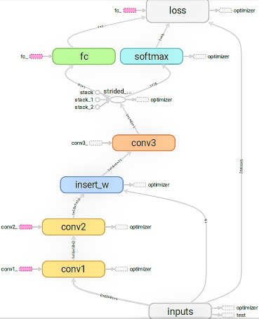
The RL trading agent feeds 𝐬𝐭subscript𝐬𝐭\mathbf{s_{t}} into the Convolutional Neural Network and plugs 𝐯𝐭subscript𝐯𝐭\mathbf{v_{t}} into the feature map tensors before the output layer. The topology of the output layer is a concatenation of a Softmax layer and fully connected layer. It outputs the predicted optimal opening portfolio weights 𝐛𝐭𝐩𝐫𝐞superscriptsubscript𝐛𝐭𝐩𝐫𝐞\mathbf{b_{t}^{pre}} and the predicted logarithmic rate of return of the tthsubscript𝑡𝑡t_{th} trading period rtpresuperscriptsubscript𝑟𝑡𝑝𝑟𝑒r_{t}^{pre} respectively.

The structure of the network is shown as Figure1.
Refer to caption
Figure 1: Topology of the Network

Filters of the network are all one-dimension for the following two reasons:

  1. 1)

    The AI trader can manage different number of stocks without changing the network architecture, and therefore enhance the flexibility of our trading system.

  2. 2)

    Due to the shared-weight architecture of CNN, the filters are trained to capture some common characteristics of the fluctuation of different stocks independently.

4.2 Trading Evaluation

After setting the opening portfolio weights of the tthsubscript𝑡𝑡t_{th} trading period to 𝐛𝐭𝐩𝐫𝐞superscriptsubscript𝐛𝐭𝐩𝐫𝐞\mathbf{b_{t}^{pre}}, the market commences, and our RL agent do not trade till the opening of next trading period (t+1)𝑡1(t+1). At the end of the tthsubscript𝑡𝑡t_{th} trading period, we can evaluate the performance of the initial portfolio weights 𝐛𝐭𝐩𝐫𝐞superscriptsubscript𝐛𝐭𝐩𝐫𝐞\mathbf{b_{t}^{pre}} and train out neural network later by calculating the logarithmic rate of return rttruesuperscriptsubscript𝑟𝑡𝑡𝑟𝑢𝑒r_{t}^{true}.

To recap, we write the formula of again:

rttrue=log(𝐛𝐭𝐩𝐫𝐞𝐗𝐭)superscriptsubscript𝑟𝑡𝑡𝑟𝑢𝑒𝑙𝑜𝑔superscriptsubscript𝐛𝐭𝐩𝐫𝐞subscript𝐗𝐭r_{t}^{true}=log(\mathbf{b_{t}^{pre}}\mathbf{X_{t}}) (8)

where 𝐗𝐭subscript𝐗𝐭\mathbf{X_{t}} is the price fluctuation vector that we introduced in section 3.1.

4.3 Training

To recap, we write the loss function here again:

L(𝜽)=𝐿𝜽absent\displaystyle L(\boldsymbol{\theta})= α(rtprerttrue)2β𝐛𝐭𝐨𝐩𝐭log(𝐛𝐭𝐩𝐫𝐞)𝛼superscriptsuperscriptsubscript𝑟𝑡𝑝𝑟𝑒superscriptsubscript𝑟𝑡𝑡𝑟𝑢𝑒2𝛽superscriptsubscript𝐛𝐭𝐨𝐩𝐭𝑙𝑜𝑔superscriptsubscript𝐛𝐭𝐩𝐫𝐞\displaystyle\alpha(r_{t}^{pre}-r_{t}^{true})^{2}-\beta\mathbf{b_{t}^{opt}}\cdot log(\mathbf{b_{t}^{pre}}) (7)
σrttrue+c𝜽𝜎superscriptsubscript𝑟𝑡𝑡𝑟𝑢𝑒𝑐norm𝜽\displaystyle-\sigma r_{t}^{true}+c||\boldsymbol{\theta}||

where α,β,σ,c>0𝛼𝛽𝜎𝑐0\alpha,\beta,\sigma,c>0 are user specified hyperparameters determining the importance of each terms in loss function. Now we explain each term in detail:

α(rtprerttrue)2𝛼superscriptsuperscriptsubscript𝑟𝑡𝑝𝑟𝑒superscriptsubscript𝑟𝑡𝑡𝑟𝑢𝑒2\alpha(r_{t}^{pre}-r_{t}^{true})^{2}: this term reflects the squared error between the network predicted logarithmic rate of return and the true logarithmic rate of return, which is calculated at the end of the tthsubscript𝑡𝑡t_{th} trading period.

β𝐛𝐭𝐨𝐩𝐭log(𝐛𝐭𝐩𝐫𝐞)𝛽superscriptsubscript𝐛𝐭𝐨𝐩𝐭𝑙𝑜𝑔superscriptsubscript𝐛𝐭𝐩𝐫𝐞-\beta\mathbf{b_{t}^{opt}}\cdot log(\mathbf{b_{t}^{pre}}): this term reflects the cross entropy between the network predicted optimal opening portfolio weights 𝐛𝐭𝐩𝐫𝐞superscriptsubscript𝐛𝐭𝐩𝐫𝐞\mathbf{b_{t}^{pre}} and the ”follow the winner” opening portfolio weights 𝐛𝐭𝐨𝐩𝐭superscriptsubscript𝐛𝐭𝐨𝐩𝐭\mathbf{b_{t}^{opt}} which is calculated by setting b(t,i)opt=1superscriptsubscript𝑏𝑡𝑖𝑜𝑝𝑡1b_{(t,i)}^{opt}=1 and b(t,j)opt=0(ji)superscriptsubscript𝑏𝑡𝑗𝑜𝑝𝑡0for-all𝑗𝑖b_{(t,j)}^{opt}=0(\forall j\not=i) where X(t,i)subscript𝑋𝑡𝑖X_{(t,i)} is largest entry in price fluctuation vector 𝐗𝐭subscript𝐗𝐭\mathbf{X_{t}} .The reason why we name 𝐛𝐭𝐨𝐩𝐭superscriptsubscript𝐛𝐭𝐨𝐩𝐭\mathbf{b_{t}^{opt}} as ”optimal” portfolio is that:

𝐛𝐭𝐨𝐩𝐭argmaxlog(𝐛𝐗𝐭)superscriptsubscript𝐛𝐭𝐨𝐩𝐭𝑙𝑜𝑔𝐛subscript𝐗𝐭\mathbf{b_{t}^{opt}}\in\mathop{\arg\max}log(\mathbf{b}\cdot\mathbf{X_{t}})

Thus, if 𝐛𝐭𝐩𝐫𝐞superscriptsubscript𝐛𝐭𝐩𝐫𝐞\mathbf{b_{t}^{pre}} is more similar to 𝐛𝐭𝐨𝐩𝐭superscriptsubscript𝐛𝐭𝐨𝐩𝐭\mathbf{b_{t}^{opt}}, then we can achieve better logarithmic rate of return rttruesuperscriptsubscript𝑟𝑡𝑡𝑟𝑢𝑒r_{t}^{true}.

σrttrue𝜎superscriptsubscript𝑟𝑡𝑡𝑟𝑢𝑒-\sigma r_{t}^{true}: this term reflects the true logarithmic rate of return in the tthsubscript𝑡𝑡t_{th} trading period as an instant reward of setting opening portfolio weights to 𝐛𝐭𝐩𝐫𝐞superscriptsubscript𝐛𝐭𝐩𝐫𝐞\mathbf{b_{t}^{pre}}. Apparently, the agent tries to maximize rttruesuperscriptsubscript𝑟𝑡𝑡𝑟𝑢𝑒r_{t}^{true}, which is the goal of our trading system, by minimizing the loss function L(𝜽)𝐿𝜽L(\boldsymbol{\theta}).

c𝜽𝑐norm𝜽c||\boldsymbol{\theta}||: This is a classical term which prevents over-fitting by L2subscript𝐿2L_{2}-norm regulation.

After each trading period ends, we need to train our network to update the latest market information. Here we use the history reexperience mechanism[4] by randomly sampling some historical trading records and use SGD algorithm with momentum to minimize the loss function on these records, that is we update the parameter 𝜽𝜽\boldsymbol{\theta} as follow:

θ:=θlL(θ)assign𝜃𝜃𝑙𝐿𝜃\theta:=\theta-l\cdot\nabla L(\theta) (9)

where l>0𝑙0l>0 is the user specified learning rate.Mechanisms like Batch Normalization [6], Optimal Initialization for Relu [8] are used to improve the model’s performance.

The purpose of random sampling is to break the correlations of consecutive samples, which is thoroughly studied in [4]. Instead of treating each sample equally as Mnih, V. et al ’s work where they use uniform distribution sampling technique, we use Poisson distribution to emphasize the recent samples as the data distribution in finance market is often non-stationary [5].

Formally, consider the training at the end of the tthsubscript𝑡𝑡t_{th} trading period. We sample the ξthsubscript𝜉𝑡\xi_{th} trading record to implement SGD algorithm, where 0<ξt0𝜉𝑡0<\xi\leq t. In our case, the random variable (tξ)𝑡𝜉(t-\xi) subjects to the Poisson distribution with parameter λ>0𝜆0\lambda>0 , that is:

(tξ)P(λ)similar-to𝑡𝜉𝑃𝜆(t-\xi)\sim P(\lambda)

5 Back Test

We use Naïve-Average, Follow-the-Winner and Follow-the-Loser as our baseline PM strategies, competing with the proposed RLOS and RLOSRL in several independent back tests. For each experiment, we randomly select 100 constituent stocks of CSI300 index (use bootstrapping sampling method) as the assets under management and the results of back tests suggest the superiority of our strategies.

5.1 Back Tests for RLOS

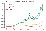
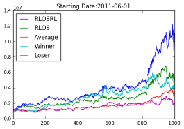
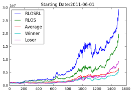
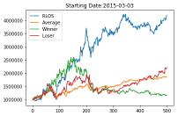
We run several back tests with different trading length on different stocks to evaluate the RLOS’s performance. We set hyperparameters N𝑁N (the maximal length of historical background for each trading period) to 20 and ρ𝜌\rho (the standard for similarity) to 0 in all the experiments. We can see clearly from back tests that RLOS outperforms all the other strategies in both short-term trading and long-term trading. We can see clearly from back tests that RLOS outperforms all the other strategies in both short-term trading and long-term trading. For all the figure below, the horizontal axis represents time and the vertical axis represents total wealth.

Refer to caption
Refer to caption
Figure 2: Trading for 500 days (RLOS)
Refer to caption
Refer to caption
Figure 3: Trading for 1000 days (RLOS)
Refer to caption
Refer to caption
Figure 4: Trading for 1500 days (RLOS)

5.2 Back Tests for RLOSRL

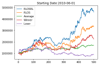
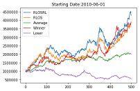
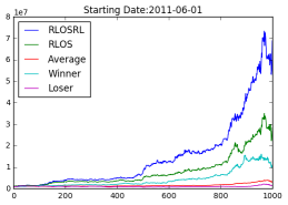
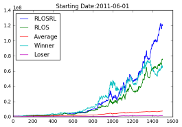
We validate the performance of RLOSRL on several back tests. The RL agent is trained on data before June 1stsuperscript1𝑠𝑡1^{st} 2010 to avoid data leakage. To some extent, the trading behaviors of RLOS and RLOSRL are similar since one of the inputs of RLSORL is the analyzed result from RLOS, while we can still see that RLOSRL is superior to RLOS in all the back tests.

Parameter Value
λ𝜆\lambda: Poisson parameter 50
r𝑟r: Momontum 0.9
α𝛼\alpha 104superscript10410^{-4}
β𝛽\beta 102superscript10210^{-2}
σ𝜎\sigma 102superscript10210^{-2}
c𝑐c 104superscript10410^{-4}
Table 1: Hyperparameter
Hundreds of Steps Learning Rate
0-500 102superscript10210^{-2}
0-1000 103superscript10310^{-3}
0-1500 104superscript10410^{-4}
Table 2: Learning Rate Decay
Refer to caption
Refer to caption
Figure 5: Trading for 500 days (RLOSRL)
Refer to caption
Refer to caption
Figure 6: Trading for 1000 days (RLOSRL)
Refer to caption
Refer to caption
Figure 7: Trading for 1500 days (RLOSRL)

6 Conclusion

In this paper, we first analyze the advantages of GLOS algorithm, which are Information-Benefit, Greed and Long-Term Superiority, and then propose the so-called RLOS algorithm, which is robust, profitable, and computationally effective, by approximating the objective function of GLOS using Taylor expansion. We further combine the RLOS with RL technique to form an ensembled strategy, where the PM agent is trained in a way to maximize the expected logarithmic rate of return of investment. The stability and profitability of our methods are empirically validated on several independent experiments. We leave some possible avenues for future exploration here:

  • \bullet

    Customize our PM strategies on other types of market. say Future, Currency, Bond etc.

  • \bullet

    Customize our PM strategies on high frequency trading.

  • \bullet

    Combine assets selection strategy with our PM strategies.

  • \bullet

    Take transaction fee into consideration.

  • \bullet

    Estimate the parameters involved in our model more precisely.

  • \bullet

    Approximate the objective function of GLOS more precisely.

References

[1] Cover, T.M. and Thomas, J.A., 2012. Elements of information theory. John Wiley & Sons. Vancouver

[2] Silver, D., Huang, A., Maddison, C.J., Guez, A., Sifre, L., Van Den Driessche, G., Schrittwieser, J., Antonoglou, I., Panneershelvam, V., Lanctot, M. and Dieleman, S., 2016. Mastering the game of Go with deep neural networks and tree search. nature, 529(7587), pp.484-489.

[3] Silver, D., Schrittwieser, J., Simonyan, K., Antonoglou, I., Huang, A., Guez, A., Hubert, T., Baker, L., Lai, M., Bolton, A. and Chen, Y., 2017. Mastering the game of go without human knowledge. Nature, 550(7676), p.354.

[4] Mnih, V., Kavukcuoglu, K., Silver, D., Rusu, A.A., Veness, J., Bellemare, M.G., Graves, A., Riedmiller, M., Fidjeland, A.K., Ostrovski, G. and Petersen, S., 2015. Human-level control through deep reinforcement learning. Nature, 518(7540), p.529.

[5] Lopez de Prado, M., 2018. The 10 Reasons Most Machine Learning Funds Fail.

[6] Ioffe, S. and Szegedy, C., 2015, June. Batch normalization: Accelerating deep network training by reducing internal covariate shift. In International conference on machine learning (pp. 448-456).

[7] Nair, V. and Hinton, G.E., 2010. Rectified linear units improve restricted boltzmann machines. In Proceedings of the 27th international conference on machine learning (ICML-10) (pp. 807-814).

[8] He, K., Zhang, X., Ren, S. and Sun, J., 2015. Delving deep into rectifiers: Surpassing human-level performance on imagenet classification. In Proceedings of the IEEE international conference on computer vision (pp. 1026-1034).

[9] Markowitz, H., 1952. Portfolio selection. The journal of finance, 7(1), pp.77-91.

[10] Algoet, P.H. and Cover, T.M., 2011. Asymptotic optimality and asymptotic equipartition properties of log-optimum investment. In THE KELLY CAPITAL GROWTH INVESTMENT CRITERION: THEORY and PRACTICE (pp. 157-179).

[11] Li, B. and Hoi, S.C., 2014. Online portfolio selection: A survey. ACM Computing Surveys (CSUR), 46(3), p.35.

[12] Ormos, M. and Urbán, A., 2013. Performance analysis of log-optimal portfolio strategies with transaction costs. Quantitative Finance, 13(10), pp.1587-1597.

[13] Vajda, I., 2006. Analysis of semi-log-optimal investment strategies. In Prague Stochastics (pp. 719-727).

[14] Jiang, Z. and Liang, J., 2016. Cryptocurrency portfolio management with deep reinforcement learning. arXiv preprint arXiv:1612.01277.

[15] Dempster, M.A. and Leemans, V., 2006. An automated FX trading system using adaptive reinforcement learning. Expert Systems with Applications, 30(3), pp.543-552.

Appendix

Appendix A Proof of Theorem 1

Lemma A.1.

E(log(ϕ(x)))log(E(ϕ(x))),r,v,x0,ϕ(x)>0.formulae-sequence𝐸𝑙𝑜𝑔italic-ϕ𝑥𝑙𝑜𝑔𝐸italic-ϕ𝑥for-all𝑟𝑣formulae-sequence𝑥0italic-ϕ𝑥0E(log(\phi(x)))\leq log(E(\phi(x))),\forall r,v,x\geq 0,\ \phi(x)>0.
Proof: Since the logarithm function satisfies

log(λx1+(1λ)x2)λlog(x1)+(1λ)log(x2),λ[0,1]formulae-sequence𝑙𝑜𝑔𝜆subscript𝑥11𝜆subscript𝑥2𝜆𝑙𝑜𝑔subscript𝑥11𝜆𝑙𝑜𝑔subscript𝑥2𝜆01log(\lambda x_{1}+(1-\lambda)x_{2})\geq\lambda log(x_{1})+(1-\lambda)log(x_{2}),\lambda\in[0,1]

which shows it is a concave function.

Let λ=x2xx2x1𝜆subscript𝑥2𝑥subscript𝑥2subscript𝑥1\lambda=\frac{x_{2}-x}{x_{2}-x_{1}}, when x[x1,x2]𝑥subscript𝑥1subscript𝑥2x\in[x_{1},x_{2}]. Then we have log(x)x2xx2x1log(x1)+xx1x2x1log(x2)𝑙𝑜𝑔𝑥subscript𝑥2𝑥subscript𝑥2subscript𝑥1𝑙𝑜𝑔subscript𝑥1𝑥subscript𝑥1subscript𝑥2subscript𝑥1𝑙𝑜𝑔subscript𝑥2log(x)\geq\frac{x_{2}-x}{x_{2}-x_{1}}log(x_{1})+\frac{x-x_{1}}{x_{2}-x_{1}}log(x_{2}).

The inequality is equivalent to

1xx1[log(x)log(x1)]1x2x1[log(x2)log(x1)]1𝑥subscript𝑥1delimited-[]𝑙𝑜𝑔𝑥𝑙𝑜𝑔subscript𝑥11subscript𝑥2subscript𝑥1delimited-[]𝑙𝑜𝑔subscript𝑥2𝑙𝑜𝑔subscript𝑥1\frac{1}{x-x_{1}}[log(x)-log(x_{1})]\geq\frac{1}{x_{2}-x_{1}}[log(x_{2})-log(x_{1})]

Let xx1𝑥subscript𝑥1x\to x_{1}, we have

(x2x1)log(x1)log(x2)log(x1)subscript𝑥2subscript𝑥1𝑙𝑜superscript𝑔subscript𝑥1𝑙𝑜𝑔subscript𝑥2𝑙𝑜𝑔subscript𝑥1(x_{2}-x_{1})log^{\prime}(x_{1})\geq log(x_{2})-log(x_{1})

Let x0=i=1mλixisubscript𝑥0subscriptsuperscript𝑚𝑖1subscript𝜆𝑖subscript𝑥𝑖x_{0}=\sum^{m}_{i=1}{\lambda}_{i}x_{i}. When i=1mλi=1,λi>0formulae-sequencesubscriptsuperscript𝑚𝑖1subscript𝜆𝑖1subscript𝜆𝑖0\sum^{m}_{i=1}{\lambda}_{i}=1,{\lambda}_{i}>0.

For each i𝑖i, we have

λi(xix0)log(x0)λi[log(xi)log(x0)]subscript𝜆𝑖subscript𝑥𝑖subscript𝑥0𝑙𝑜superscript𝑔subscript𝑥0subscript𝜆𝑖delimited-[]𝑙𝑜𝑔subscript𝑥𝑖𝑙𝑜𝑔subscript𝑥0{\lambda}_{i}(x_{i}-x_{0})log^{\prime}(x_{0})\geq{\lambda}_{i}[log(x_{i})-log(x_{0})]

Thus

i=1mλi(xix0)log(x0)i=1mλi[log(xi)log(x0)]superscriptsubscript𝑖1𝑚subscript𝜆𝑖subscript𝑥𝑖subscript𝑥0𝑙𝑜superscript𝑔subscript𝑥0superscriptsubscript𝑖1𝑚subscript𝜆𝑖delimited-[]𝑙𝑜𝑔subscript𝑥𝑖𝑙𝑜𝑔subscript𝑥0\sum_{i=1}^{m}{\lambda}_{i}(x_{i}-x_{0})log^{\prime}(x_{0})\geq\sum_{i=1}^{m}{\lambda}_{i}[log(x_{i})-log(x_{0})]

Since

E(log(ϕ(x)))𝐸𝑙𝑜𝑔italic-ϕ𝑥\displaystyle E(log(\phi(x))) =log(ϕ(x))𝑑F(x)absent𝑙𝑜𝑔italic-ϕ𝑥differential-d𝐹𝑥\displaystyle=\int log(\phi(x))dF(x)
=limtk=1log(ϕ(xk))(F(kn)F(k1n))absentsubscript𝑡superscriptsubscript𝑘1𝑙𝑜𝑔italic-ϕsubscript𝑥𝑘𝐹𝑘𝑛𝐹𝑘1𝑛\displaystyle=\lim\limits_{t\to\infty}\sum_{k=1}^{\infty}log(\phi(x_{k}))(F(\frac{k}{n})-F(\frac{k-1}{n}))
log(E(ϕ(x))\displaystyle log(E(\phi(x)) =log(ϕ(x)𝑑F(x))absent𝑙𝑜𝑔italic-ϕ𝑥differential-d𝐹𝑥\displaystyle=log(\int\phi(x)dF(x))
=log(limtk=1ϕ(xk)(F(kn)F(k1n))\displaystyle=log(\lim\limits_{t\to\infty}\sum_{k=1}^{\infty}\phi(x_{k})(F(\frac{k}{n})-F(\frac{k-1}{n}))

and the logarithm function is continuous, let λk=F(kn)F(k1n),mformulae-sequencesubscript𝜆𝑘𝐹𝑘𝑛𝐹𝑘1𝑛𝑚{\lambda}_{k}=F(\frac{k}{n})-F(\frac{k-1}{n}),m\to\infty, then we have

log(ϕ(x))𝑑F(x)log(ϕ(x)𝑑F(x))𝑙𝑜𝑔italic-ϕ𝑥differential-d𝐹𝑥𝑙𝑜𝑔italic-ϕ𝑥differential-d𝐹𝑥\int log(\phi(x))dF(x)\leq log(\int\phi(x)dF(x))

So E(log(ϕ(x)))log(E(ϕ(x)))𝐸𝑙𝑜𝑔italic-ϕ𝑥𝑙𝑜𝑔𝐸italic-ϕ𝑥E(log(\phi(x)))\leq log(E(\phi(x))) as desired.

Lemma A.2.

If bsuperscript𝑏b^{*} is the optimal portfolio and EbTXbTX𝐸superscript𝑏𝑇𝑋superscript𝑏superscript𝑇𝑋E\frac{b^{T}X}{b^{*^{T}}X} exists, we have EbTXbTX1𝐸superscript𝑏𝑇𝑋superscript𝑏superscript𝑇𝑋1E\frac{b^{T}X}{b^{*^{T}}X}\leq 1, for any other portfolio b𝑏b.
Proof: Let W(bλ,F)=log(bλTx)𝑑F(x),bλ=λb+(1λ)bformulae-sequence𝑊subscript𝑏𝜆𝐹𝑙𝑜𝑔superscriptsubscript𝑏𝜆𝑇𝑥differential-d𝐹𝑥subscript𝑏𝜆𝜆𝑏1𝜆superscript𝑏W(b_{\lambda},F)=\int log(b_{\lambda}^{T}x)dF(x),b_{\lambda}=\lambda b+(1-\lambda)b^{*}, where b𝑏b is another portfolio. When λ=0𝜆0\lambda=0, we have b0=bsubscript𝑏0superscript𝑏b_{0}=b^{*}.

According to the definition we have the greatest value

W(b0,F)=W(b,F)=maxbAlog(bTx)𝑑F(x)𝑊subscript𝑏0𝐹𝑊superscript𝑏𝐹subscript𝑏𝐴𝑙𝑜𝑔superscript𝑏𝑇𝑥differential-d𝐹𝑥W(b_{0},F)=W(b^{*},F)=\mathop{\max}_{b\in A}\int log(b^{T}x)dF(x)

We say W(b0,F)W(bk,F),k[0,1]formulae-sequence𝑊subscript𝑏0𝐹𝑊subscript𝑏𝑘𝐹for-all𝑘01W(b_{0},F)\geq W(b_{k},F),\forall k\in[0,1] and dW(bλ,F)dλ0𝑑𝑊subscript𝑏𝜆𝐹𝑑𝜆0\frac{dW(b_{\lambda},F)}{d\lambda}\leq 0 when λ0𝜆0\lambda\to 0 by the definition of derivative.

That is to say,

limλ0+dW(bλ,F)dλsubscript𝜆subscript0𝑑𝑊subscript𝑏𝜆𝐹𝑑𝜆\displaystyle\lim\limits_{\lambda\to 0_{+}}\frac{dW(b_{\lambda},F)}{d\lambda} =limλ0+1λ[W(bλ,F)W(b0,F)]absentsubscript𝜆subscript01𝜆delimited-[]𝑊subscript𝑏𝜆𝐹𝑊subscript𝑏0𝐹\displaystyle=\lim\limits_{\lambda\to 0_{+}}\frac{1}{\lambda}[W(b_{\lambda},F)-W(b_{0},F)]
=limλ0+1λ[E(log(λbTX)+(1λ)bTX))E(log(bTX))]\displaystyle=\lim\limits_{\lambda\to 0_{+}}\frac{1}{\lambda}[E(log(\lambda b^{T}X)+(1-\lambda)b^{*^{T}}X))-E(log(b^{*^{T}}X))]
=E(limλ0+1λlog(λbTXbTX+1λ))()absent𝐸subscript𝜆subscript01𝜆𝑙𝑜𝑔𝜆superscript𝑏𝑇𝑋superscript𝑏superscript𝑇𝑋1𝜆\displaystyle=E(\lim\limits_{\lambda\to 0_{+}}\frac{1}{\lambda}log(\lambda\frac{b^{T}X}{b^{*^{T}}X}+1-\lambda))\qquad(*)
=E(limλ0+1λlog(1+λ(bTXbTX1)))absent𝐸subscript𝜆subscript01𝜆𝑙𝑜𝑔1𝜆superscript𝑏𝑇𝑋superscript𝑏superscript𝑇𝑋1\displaystyle=E(\lim\limits_{\lambda\to 0_{+}}\frac{1}{\lambda}log(1+\lambda(\frac{b^{T}X}{b^{*^{T}}X}-1)))
=E(bTXbTX1)()\displaystyle=E(\frac{b^{T}X}{b^{*^{T}}X}-1)\qquad(**)
0absent0\displaystyle\leq 0

The equality (*) can be referred to [5] and the equality (**) is due to the L’Hospital’s rule.

Then we will give the proof of Theorem 1.

The Proof of Theorem 1:

ΔVYΔsubscript𝑉𝑌\displaystyle\Delta V_{Y} =r𝐗|Y(𝐛𝐗|YT𝐱)r𝐗|Y(𝐛𝐗T𝐱)absentsubscript𝑟conditional𝐗𝑌superscriptsubscript𝐛conditional𝐗𝑌superscript𝑇𝐱subscript𝑟conditional𝐗𝑌superscriptsubscript𝐛𝐗superscript𝑇𝐱\displaystyle=r_{\mathbf{X}|Y}(\mathbf{b}_{\mathbf{X}|Y}^{*^{T}}\mathbf{x})-r_{\mathbf{X}|Y}(\mathbf{b}_{\mathbf{X}}^{*^{T}}\mathbf{x})
=log(𝐛𝐗|YT𝐱)𝑑F(𝐱|Y=y)log(𝐛𝐗T𝐱)𝑑F(𝐱|Y=y)absent𝑙𝑜𝑔superscriptsubscript𝐛conditional𝐗𝑌superscript𝑇𝐱differential-d𝐹conditional𝐱𝑌𝑦𝑙𝑜𝑔superscriptsubscript𝐛𝐗superscript𝑇𝐱differential-d𝐹conditional𝐱𝑌𝑦\displaystyle=\int log(\mathbf{b}_{\mathbf{X}|Y}^{*^{T}}\mathbf{x})dF(\mathbf{x}|Y=y)-\int log(\mathbf{b}_{\mathbf{X}}^{*^{T}}\mathbf{x})dF(\mathbf{x}|Y=y)
=log𝐛𝐗|YT𝐱𝐛𝐗T𝐱𝑑F(𝐱|Y=y)absent𝑙𝑜𝑔superscriptsubscript𝐛conditional𝐗𝑌superscript𝑇𝐱superscriptsubscript𝐛𝐗superscript𝑇𝐱differential-d𝐹conditional𝐱𝑌𝑦\displaystyle=\int log\frac{\mathbf{b}_{\mathbf{X}|Y}^{*^{T}}\mathbf{x}}{\mathbf{b}_{\mathbf{X}}^{*^{T}}\mathbf{x}}dF(\mathbf{x}|Y=y)
=log(𝐛𝐗|YT𝐱𝐛𝐗T𝐱f(𝐱)f𝐱|Y=y(𝐱))𝑑F(𝐱|Y=y)+logf(𝐱)f𝐱|Y=y(𝐱)𝑑F(𝐱|Y=y)absent𝑙𝑜𝑔superscriptsubscript𝐛conditional𝐗𝑌superscript𝑇𝐱superscriptsubscript𝐛𝐗superscript𝑇𝐱𝑓𝐱subscript𝑓conditional𝐱𝑌𝑦𝐱differential-d𝐹conditional𝐱𝑌𝑦𝑙𝑜𝑔𝑓𝐱subscript𝑓conditional𝐱𝑌𝑦𝐱differential-d𝐹conditional𝐱𝑌𝑦\displaystyle=\int log(\frac{\mathbf{b}_{\mathbf{X}|Y}^{*^{T}}\mathbf{x}}{\mathbf{b}_{\mathbf{X}}^{*^{T}}\mathbf{x}}\cdot\frac{f(\mathbf{x})}{f_{\mathbf{x}|Y=y}(\mathbf{x})})dF(\mathbf{x}|Y=y)+\int log\frac{f(\mathbf{x})}{f_{\mathbf{x}|Y=y}(\mathbf{x})}dF(\mathbf{x}|Y=y)
=log(𝐛𝐗|YT𝐱𝐛𝐗T𝐱f(𝐱)f𝐱|Y=y(𝐱))𝑑F(𝐱|Y=y)+f𝐱|Y=y(𝐱)logf(𝐱)f𝐱|Y=y(𝐱)𝑑𝐱absent𝑙𝑜𝑔superscriptsubscript𝐛conditional𝐗𝑌superscript𝑇𝐱superscriptsubscript𝐛𝐗superscript𝑇𝐱𝑓𝐱subscript𝑓conditional𝐱𝑌𝑦𝐱differential-d𝐹conditional𝐱𝑌𝑦subscript𝑓conditional𝐱𝑌𝑦𝐱𝑙𝑜𝑔𝑓𝐱subscript𝑓conditional𝐱𝑌𝑦𝐱differential-d𝐱\displaystyle=\int log(\frac{\mathbf{b}_{\mathbf{X}|Y}^{*^{T}}\mathbf{x}}{\mathbf{b}_{\mathbf{X}}^{*^{T}}\mathbf{x}}\cdot\frac{f(\mathbf{x})}{f_{\mathbf{x}|Y=y}(\mathbf{x})})dF(\mathbf{x}|Y=y)+\int f_{\mathbf{x}|Y=y}(\mathbf{x})log\frac{f(\mathbf{x})}{f_{\mathbf{x}|Y=y}(\mathbf{x})}d\mathbf{x}
log𝐛𝐗|YT𝐱𝐛𝐗T𝐱f(𝐱)f𝐱|Y=y(𝐱)𝑑F(𝐱|Y=y)+f𝐱|Y=y(𝐱)logf(𝐱)f𝐱|Y=y(𝐱)𝑑𝐱(lemma1)absent𝑙𝑜𝑔superscriptsubscript𝐛conditional𝐗𝑌superscript𝑇𝐱superscriptsubscript𝐛𝐗superscript𝑇𝐱𝑓𝐱subscript𝑓conditional𝐱𝑌𝑦𝐱differential-d𝐹conditional𝐱𝑌𝑦subscript𝑓conditional𝐱𝑌𝑦𝐱𝑙𝑜𝑔𝑓𝐱subscript𝑓conditional𝐱𝑌𝑦𝐱differential-d𝐱𝑙𝑒𝑚𝑚𝑎1\displaystyle\leq log\int\frac{\mathbf{b}_{\mathbf{X}|Y}^{*^{T}}\mathbf{x}}{\mathbf{b}_{\mathbf{X}}^{*^{T}}\mathbf{x}}\cdot\frac{f(\mathbf{x})}{f_{\mathbf{x}|Y=y}(\mathbf{x})}dF(\mathbf{x}|Y=y)+\int f_{\mathbf{x}|Y=y}(\mathbf{x})log\frac{f(\mathbf{x})}{f_{\mathbf{x}|Y=y}(\mathbf{x})}d\mathbf{x}\qquad(lemma1)
=log𝐛𝐗|YT𝐱𝐛𝐗T𝐱𝑑F(𝐱)+f𝐱|Y=y(𝐱)logf(𝐱)f𝐱|Y=y(𝐱)𝑑𝐱absent𝑙𝑜𝑔superscriptsubscript𝐛conditional𝐗𝑌superscript𝑇𝐱superscriptsubscript𝐛𝐗superscript𝑇𝐱differential-d𝐹𝐱subscript𝑓conditional𝐱𝑌𝑦𝐱𝑙𝑜𝑔𝑓𝐱subscript𝑓conditional𝐱𝑌𝑦𝐱differential-d𝐱\displaystyle=log\int\frac{\mathbf{b}_{\mathbf{X}|Y}^{*^{T}}\mathbf{x}}{\mathbf{b}_{\mathbf{X}}^{*^{T}}\mathbf{x}}dF(\mathbf{x})+\int f_{\mathbf{x}|Y=y}(\mathbf{x})log\frac{f(\mathbf{x})}{f_{\mathbf{x}|Y=y}(\mathbf{x})}d\mathbf{x}
log1+f𝐱|Y=y(𝐱)logf(𝐱)f𝐱|Y=y(𝐱)𝑑𝐱(lemma2)absent𝑙𝑜𝑔1subscript𝑓conditional𝐱𝑌𝑦𝐱𝑙𝑜𝑔𝑓𝐱subscript𝑓conditional𝐱𝑌𝑦𝐱differential-d𝐱𝑙𝑒𝑚𝑚𝑎2\displaystyle\leq log1+\int f_{\mathbf{x}|Y=y}(\mathbf{x})log\frac{f(\mathbf{x})}{f_{\mathbf{x}|Y=y}(\mathbf{x})}d\mathbf{x}\qquad(lemma2)
=f𝐱|Y=y(𝐱)logf(𝐱)f𝐱|Y=y(𝐱)𝑑𝐱absentsubscript𝑓conditional𝐱𝑌𝑦𝐱𝑙𝑜𝑔𝑓𝐱subscript𝑓conditional𝐱𝑌𝑦𝐱differential-d𝐱\displaystyle=\int f_{\mathbf{x}|Y=y}(\mathbf{x})log\frac{f(\mathbf{x})}{f_{\mathbf{x}|Y=y}(\mathbf{x})}d\mathbf{x}

Furthermore, we define ΔV=E(ΔVY)Δ𝑉𝐸Δsubscript𝑉𝑌\Delta V=E(\Delta V_{Y}), the expectation of the increment ΔVYΔsubscript𝑉𝑌\Delta V_{Y} with respect to Y𝑌Y. Then we will prove ΔVΔ𝑉\Delta V also has an upper bound. Denote by G(H)𝐺𝐻G(H) the cumulative distribution function of Y((X,Y))𝑌𝑋𝑌Y((X,Y)), and g(h)𝑔g(h) the density function of Y((X,Y))𝑌𝑋𝑌Y((X,Y)), we verify that

ΔVΔ𝑉\displaystyle\Delta V =ΔVY=y𝑑G(y)absentΔsubscript𝑉𝑌𝑦differential-d𝐺𝑦\displaystyle=\int\Delta V_{Y=y}dG(y)
f𝐱|Y=ylogf𝐱|Y=yf(𝐱)𝑑𝐱𝑑G(y)absentdouble-integralsubscript𝑓conditional𝐱𝑌𝑦𝑙𝑜𝑔subscript𝑓conditional𝐱𝑌𝑦𝑓𝐱differential-d𝐱differential-d𝐺𝑦\displaystyle\leq\iint f_{\mathbf{x}|Y=y}log\frac{f_{\mathbf{x}|Y=y}}{f(\mathbf{x})}d\mathbf{x}dG(y)
=f𝐱|Y=yg(y)logf𝐱|Y=yg(y)f(𝐱)g(y)𝑑𝐱𝑑yabsentdouble-integralsubscript𝑓conditional𝐱𝑌𝑦𝑔𝑦𝑙𝑜𝑔subscript𝑓conditional𝐱𝑌𝑦𝑔𝑦𝑓𝐱𝑔𝑦differential-d𝐱differential-d𝑦\displaystyle=\iint f_{\mathbf{x}|Y=y}\cdot g(y)log\frac{f_{\mathbf{x}|Y=y}g(y)}{f(\mathbf{x})g(y)}d\mathbf{x}dy
=h(𝐱,y)logh(𝐱,y)f(𝐱)g(y)𝑑𝐱𝑑yabsentdouble-integral𝐱𝑦𝑙𝑜𝑔𝐱𝑦𝑓𝐱𝑔𝑦differential-d𝐱differential-d𝑦\displaystyle=\iint h(\mathbf{x},y)log\frac{h(\mathbf{x},y)}{f(\mathbf{x})g(y)}d\mathbf{x}dy

Appendix B Proof of Theorem 2

Proof:

According to lemma 2, we have ESnSn1𝐸subscript𝑆𝑛superscriptsubscript𝑆𝑛1E\frac{S_{n}}{S_{n}^{*}}\leq 1 and

Pr(Sn>n2Sn)𝑃𝑟subscript𝑆𝑛superscript𝑛2superscriptsubscript𝑆𝑛\displaystyle Pr(S_{n}>n^{2}S_{n}^{*}) =Pr(SnSn>n2)absent𝑃𝑟subscript𝑆𝑛superscriptsubscript𝑆𝑛superscript𝑛2\displaystyle=Pr(\frac{S_{n}}{S_{n}^{*}}>n^{2})
=n2+𝑑F(SnSn)absentsuperscriptsubscriptsuperscript𝑛2differential-d𝐹subscript𝑆𝑛superscriptsubscript𝑆𝑛\displaystyle=\int_{n^{2}}^{+\infty}dF(\frac{S_{n}}{S_{n}^{*}})
1n2n2+SnSn𝑑F(SnSn)absent1superscript𝑛2superscriptsubscriptsuperscript𝑛2subscript𝑆𝑛superscriptsubscript𝑆𝑛differential-d𝐹subscript𝑆𝑛superscriptsubscript𝑆𝑛\displaystyle\leq\frac{1}{n^{2}}\int_{n^{2}}^{+\infty}\frac{S_{n}}{S_{n}^{*}}dF(\frac{S_{n}}{S_{n}^{*}})
1n20+SnSn𝑑F(SnSn)absent1superscript𝑛2superscriptsubscript0subscript𝑆𝑛superscriptsubscript𝑆𝑛differential-d𝐹subscript𝑆𝑛superscriptsubscript𝑆𝑛\displaystyle\leq\frac{1}{n^{2}}\int_{0}^{+\infty}\frac{S_{n}}{S_{n}^{*}}dF(\frac{S_{n}}{S_{n}^{*}})
1n2ESnSnabsent1superscript𝑛2𝐸subscript𝑆𝑛superscriptsubscript𝑆𝑛\displaystyle\leq\frac{1}{n^{2}}E\frac{S_{n}}{S_{n}^{*}}
1n2absent1superscript𝑛2\displaystyle\leq\frac{1}{n^{2}}

That is to say,

Pr(1nlogSnSn>1nlogn2)1n2𝑃𝑟1𝑛𝑙𝑜𝑔subscript𝑆𝑛superscriptsubscript𝑆𝑛1𝑛𝑙𝑜𝑔superscript𝑛21superscript𝑛2Pr(\frac{1}{n}log\frac{S_{n}}{S_{n}^{*}}>\frac{1}{n}logn^{2})\leq\frac{1}{n^{2}}
n=1Pr(1nlogSnSn>2lognn)n=11n2<superscriptsubscript𝑛1𝑃𝑟1𝑛𝑙𝑜𝑔subscript𝑆𝑛superscriptsubscript𝑆𝑛2𝑙𝑜𝑔𝑛𝑛subscript𝑛11superscript𝑛2\sum_{n=1}^{\infty}Pr(\frac{1}{n}log\frac{S_{n}}{S_{n}^{*}}>\frac{2logn}{n})\leq\sum_{n=1}{\infty}\frac{1}{n^{2}}<\infty

and

Pr(limn¯{1nlogSnSn>2lognn)})\displaystyle Pr(\overline{\lim\limits_{n\to\infty}}\{\frac{1}{n}log\frac{S_{n}}{S_{n}^{*}}>\frac{2logn}{n})\}) =limkPr(n=k{1nlogSnSn})absentsubscript𝑘𝑃𝑟superscriptsubscript𝑛𝑘1𝑛𝑙𝑜𝑔subscript𝑆𝑛superscriptsubscript𝑆𝑛\displaystyle=\lim\limits_{k\to\infty}Pr(\bigcup_{n=k}^{\infty}\{\frac{1}{n}log\frac{S_{n}}{S_{n}^{*}}\})
limkn=kPr({1nlogSnSn})absentsubscript𝑘subscript𝑛𝑘𝑃𝑟1𝑛𝑙𝑜𝑔subscript𝑆𝑛superscriptsubscript𝑆𝑛\displaystyle\leq\lim\limits_{k\to\infty}\sum_{n=k}Pr(\{\frac{1}{n}log\frac{S_{n}}{S_{n}^{*}}\})
=0absent0\displaystyle=0

This implies, N>0,n>Nformulae-sequence𝑁0for-all𝑛𝑁\exists N>0,\forall n>N, we have

1nlogSnSn2lognn1𝑛𝑙𝑜𝑔subscript𝑆𝑛superscriptsubscript𝑆𝑛2𝑙𝑜𝑔𝑛𝑛\frac{1}{n}log\frac{S_{n}}{S_{n}^{*}}\leq\frac{2logn}{n}

Thus, we have limn¯1nlogSnSn0,withprobability 1¯subscript𝑛1𝑛𝑙𝑜𝑔subscript𝑆𝑛superscriptsubscript𝑆𝑛0𝑤𝑖𝑡𝑝𝑟𝑜𝑏𝑎𝑏𝑖𝑙𝑖𝑡𝑦1\overline{\lim\limits_{n\to\infty}}\frac{1}{n}log\frac{S_{n}}{S_{n}^{*}}\leq 0,with\ probability\ 1 as desired and conclude that Snsuperscriptsubscript𝑆𝑛S_{n}^{*} is asymptotically superior to Snsubscript𝑆𝑛S_{n}.

Appendix C Computation of Taylor Expansion

Elog(𝐛T𝐗)𝐸𝑙𝑜𝑔superscript𝐛𝑇𝐗\displaystyle Elog(\mathbf{b}^{T}\mathbf{X}) (4)
\displaystyle\approx E(logE(𝐛T𝐗)+𝐛T𝐗E(𝐛T𝐗)E(𝐛T𝐗)(𝐛T𝐗E(𝐛T𝐗))22(E(𝐛T𝐗))2)𝐸𝑙𝑜𝑔𝐸superscript𝐛𝑇𝐗superscript𝐛𝑇𝐗𝐸superscript𝐛𝑇𝐗𝐸superscript𝐛𝑇𝐗superscriptsuperscript𝐛𝑇𝐗𝐸superscript𝐛𝑇𝐗22superscript𝐸superscript𝐛𝑇𝐗2\displaystyle E(logE(\mathbf{b}^{T}\mathbf{X})+\frac{\mathbf{b}^{T}\mathbf{X}-E(\mathbf{b}^{T}\mathbf{X})}{E(\mathbf{b}^{T}\mathbf{X})}-\frac{(\mathbf{b}^{T}\mathbf{X}-E(\mathbf{b}^{T}\mathbf{X}))^{2}}{2(E(\mathbf{b}^{T}\mathbf{X}))^{2}})
=\displaystyle= log(𝐛T𝝁)12(𝐛T𝝁)2𝐛T𝚺𝐛𝑙𝑜𝑔superscript𝐛𝑇𝝁12superscriptsuperscript𝐛𝑇𝝁2superscript𝐛𝑇𝚺𝐛\displaystyle log(\mathbf{b}^{T}\boldsymbol{\mu})-\frac{1}{2(\mathbf{b}^{T}\boldsymbol{\mu})^{2}}\mathbf{b}^{T}\mathbf{\Sigma}\mathbf{b}

Appendix D Proof of Theorem 3

Lemma D.1.

p,q,q1,q2for-all𝑝𝑞subscript𝑞1subscript𝑞2\forall p,q,q_{1},q_{2}\in\mathbb{R}, satisfying q1qq2subscript𝑞1𝑞subscript𝑞2q_{1}\leq q\leq q_{2}, we have

|pq|maxpq,q2p𝑝𝑞𝑝𝑞subscript𝑞2𝑝|p-q|\leq\max{p-q,q_{2}-p}

Proof: If pq,pq1pq0formulae-sequencepqpsubscriptq1pq0p\geq q,p-q_{1}\geq p-q\geq 0, which refers to pq1>|pq|psubscriptq1pqp-q_{1}>|p-q|.

If p<q,q2pqp>0formulae-sequence𝑝𝑞subscript𝑞2𝑝𝑞𝑝0p<q,q_{2}-p\geq q-p>0, which refers to q2p>|pq|subscript𝑞2𝑝𝑝𝑞q_{2}-p>|p-q|.

we then prove that |pq|maxpq,q2p𝑝𝑞𝑝𝑞subscript𝑞2𝑝|p-q|\leq\max{p-q,q_{2}-p}.

Next, we will study the deviation between M(𝐛^𝐨𝐩𝐭,𝝁^,𝚺^)𝑀superscript^𝐛𝐨𝐩𝐭bold-^𝝁bold-^𝚺M(\mathbf{\hat{b}^{opt}},\boldsymbol{\hat{\mu}},\boldsymbol{\hat{\Sigma}}) and M(𝐛^𝐨𝐩𝐭,𝝁,𝚺)𝑀superscript^𝐛𝐨𝐩𝐭𝝁𝚺M(\mathbf{\hat{b}^{opt}},\boldsymbol{\mu},\boldsymbol{\Sigma}).

|M(𝐛^𝐨𝐩𝐭,𝝁^,𝚺^)M(𝐛^𝐨𝐩𝐭,𝝁,𝚺)|𝑀superscript^𝐛𝐨𝐩𝐭bold-^𝝁bold-^𝚺𝑀superscript^𝐛𝐨𝐩𝐭𝝁𝚺\displaystyle|M(\mathbf{\hat{b}^{opt}},\boldsymbol{\hat{\mu}},\boldsymbol{\hat{\Sigma}})-M(\mathbf{\hat{b}^{opt}},\boldsymbol{\mu},\boldsymbol{\Sigma})|
=\displaystyle= |log(𝐛^𝐨𝐩𝐭𝐓𝝁^)12(𝐛^𝐨𝐩𝐭𝐓𝝁^)2𝐛^𝐨𝐩𝐭𝐓𝚺^𝐛^𝐨𝐩𝐭log(𝐛^𝐨𝐩𝐭𝐓𝝁)+12(𝐛^𝐨𝐩𝐭𝐓𝝁)2𝐛^𝐨𝐩𝐭𝐓𝚺𝐛^𝐨𝐩𝐭|𝑙𝑜𝑔superscript^𝐛superscript𝐨𝐩𝐭𝐓bold-^𝝁12superscriptsuperscript^𝐛superscript𝐨𝐩𝐭𝐓bold-^𝝁2superscript^𝐛superscript𝐨𝐩𝐭𝐓bold-^𝚺superscript^𝐛𝐨𝐩𝐭𝑙𝑜𝑔superscript^𝐛superscript𝐨𝐩𝐭𝐓𝝁12superscriptsuperscript^𝐛superscript𝐨𝐩𝐭𝐓𝝁2superscript^𝐛superscript𝐨𝐩𝐭𝐓𝚺superscript^𝐛𝐨𝐩𝐭\displaystyle|log(\mathbf{\hat{b}^{{opt}^{T}}}\boldsymbol{\hat{\mu}})-\frac{1}{2(\mathbf{\hat{b}^{{opt}^{T}}}\boldsymbol{\hat{\mu}})^{2}}\mathbf{\hat{b}^{{opt}^{T}}}\boldsymbol{\hat{\Sigma}}\mathbf{\hat{b}^{opt}}-log(\mathbf{\hat{b}^{{opt}^{T}}}\boldsymbol{\mu})+\frac{1}{2(\mathbf{\hat{b}^{{opt}^{T}}}\boldsymbol{\mu})^{2}}\mathbf{\hat{b}^{{opt}^{T}}}\boldsymbol{\Sigma}\mathbf{\hat{b}^{opt}}|
=\displaystyle= |(log(𝐛^𝐨𝐩𝐭𝐓𝝁^)log(𝐛^𝐨𝐩𝐭𝐓𝝁))+(12(𝐛^𝐨𝐩𝐭𝐓𝝁)2𝐛^𝐨𝐩𝐭𝐓𝚺𝐛^𝐨𝐩𝐭12(𝐛^𝐨𝐩𝐭𝐓𝝁^)2𝐛^𝐨𝐩𝐭𝐓𝚺^𝐛^𝐨𝐩𝐭)|𝑙𝑜𝑔superscript^𝐛superscript𝐨𝐩𝐭𝐓bold-^𝝁𝑙𝑜𝑔superscript^𝐛superscript𝐨𝐩𝐭𝐓𝝁12superscriptsuperscript^𝐛superscript𝐨𝐩𝐭𝐓𝝁2superscript^𝐛superscript𝐨𝐩𝐭𝐓𝚺superscript^𝐛𝐨𝐩𝐭12superscriptsuperscript^𝐛superscript𝐨𝐩𝐭𝐓bold-^𝝁2superscript^𝐛superscript𝐨𝐩𝐭𝐓bold-^𝚺superscript^𝐛𝐨𝐩𝐭\displaystyle|(log(\mathbf{\hat{b}^{{opt}^{T}}}\boldsymbol{\hat{\mu}})-log(\mathbf{\hat{b}^{{opt}^{T}}}\boldsymbol{\mu}))+(\frac{1}{2(\mathbf{\hat{b}^{{opt}^{T}}}\boldsymbol{\mu})^{2}}\mathbf{\hat{b}^{{opt}^{T}}}\boldsymbol{\Sigma}\mathbf{\hat{b}^{opt}}-\frac{1}{2(\mathbf{\hat{b}^{{opt}^{T}}}\boldsymbol{\hat{\mu}})^{2}}\mathbf{\hat{b}^{{opt}^{T}}}\boldsymbol{\hat{\Sigma}}\mathbf{\hat{b}^{opt}})|
\displaystyle\leq |log(𝐛^𝐨𝐩𝐭𝐓𝝁^)log(𝐛^𝐨𝐩𝐭𝐓𝝁)|+|12(𝐛^𝐨𝐩𝐭𝐓𝝁)2𝐛^𝐨𝐩𝐭𝐓𝚺𝐛^𝐨𝐩𝐭12(𝐛^𝐨𝐩𝐭𝐓𝝁^)2𝐛^𝐨𝐩𝐭𝐓𝚺^𝐛^𝐨𝐩𝐭|𝑙𝑜𝑔superscript^𝐛superscript𝐨𝐩𝐭𝐓bold-^𝝁𝑙𝑜𝑔superscript^𝐛superscript𝐨𝐩𝐭𝐓𝝁12superscriptsuperscript^𝐛superscript𝐨𝐩𝐭𝐓𝝁2superscript^𝐛superscript𝐨𝐩𝐭𝐓𝚺superscript^𝐛𝐨𝐩𝐭12superscriptsuperscript^𝐛superscript𝐨𝐩𝐭𝐓bold-^𝝁2superscript^𝐛superscript𝐨𝐩𝐭𝐓bold-^𝚺superscript^𝐛𝐨𝐩𝐭\displaystyle|log(\mathbf{\hat{b}^{{opt}^{T}}}\boldsymbol{\hat{\mu}})-log(\mathbf{\hat{b}^{{opt}^{T}}}\boldsymbol{\mu})|+|\frac{1}{2(\mathbf{\hat{b}^{{opt}^{T}}}\boldsymbol{\mu})^{2}}\mathbf{\hat{b}^{{opt}^{T}}}\boldsymbol{\Sigma}\mathbf{\hat{b}^{opt}}-\frac{1}{2(\mathbf{\hat{b}^{{opt}^{T}}}\boldsymbol{\hat{\mu}})^{2}}\mathbf{\hat{b}^{{opt}^{T}}}\boldsymbol{\hat{\Sigma}}\mathbf{\hat{b}^{opt}}|
=\displaystyle= |log(𝐛^𝐨𝐩𝐭𝐓𝝁^𝐛^𝐨𝐩𝐭𝐓𝝁)|+12|1(𝐛^𝐨𝐩𝐭𝐓𝝁)2𝐛^𝐨𝐩𝐭𝐓𝚺𝐛^𝐨𝐩𝐭1(𝐛^𝐨𝐩𝐭𝐓𝝁^)2𝐛^𝐨𝐩𝐭𝐓𝚺^𝐛^𝐨𝐩𝐭|𝑙𝑜𝑔superscript^𝐛superscript𝐨𝐩𝐭𝐓bold-^𝝁superscript^𝐛superscript𝐨𝐩𝐭𝐓𝝁121superscriptsuperscript^𝐛superscript𝐨𝐩𝐭𝐓𝝁2superscript^𝐛superscript𝐨𝐩𝐭𝐓𝚺superscript^𝐛𝐨𝐩𝐭1superscriptsuperscript^𝐛superscript𝐨𝐩𝐭𝐓bold-^𝝁2superscript^𝐛superscript𝐨𝐩𝐭𝐓bold-^𝚺superscript^𝐛𝐨𝐩𝐭\displaystyle|log(\frac{\mathbf{\hat{b}^{{opt}^{T}}}\boldsymbol{\hat{\mu}}}{\mathbf{\hat{b}^{{opt}^{T}}}\boldsymbol{\mu}})|+\frac{1}{2}|\frac{1}{(\mathbf{\hat{b}^{{opt}^{T}}}\boldsymbol{\mu})^{2}}\mathbf{\hat{b}^{{opt}^{T}}}\boldsymbol{\Sigma}\mathbf{\hat{b}^{opt}}-\frac{1}{(\mathbf{\hat{b}^{{opt}^{T}}}\boldsymbol{\hat{\mu}})^{2}}\mathbf{\hat{b}^{{opt}^{T}}}\boldsymbol{\hat{\Sigma}}\mathbf{\hat{b}^{opt}}|
\displaystyle\leq |log(𝐛^𝐨𝐩𝐭𝐓𝝁^𝐛^𝐨𝐩𝐭𝐓𝝁)|+12|1(𝐛^𝐨𝐩𝐭𝐓𝝁)2𝐛^𝐨𝐩𝐭𝐓𝚺𝐛^𝐨𝐩𝐭1(𝐛^𝐨𝐩𝐭𝐓𝝁^)2𝐛^𝐨𝐩𝐭𝐓𝚺^𝐛^𝐨𝐩𝐭|𝑙𝑜𝑔superscript^𝐛superscript𝐨𝐩𝐭𝐓bold-^𝝁superscript^𝐛superscript𝐨𝐩𝐭𝐓𝝁121superscriptsuperscript^𝐛superscript𝐨𝐩𝐭𝐓𝝁2superscript^𝐛superscript𝐨𝐩𝐭𝐓𝚺superscript^𝐛𝐨𝐩𝐭1superscriptsuperscript^𝐛superscript𝐨𝐩𝐭𝐓bold-^𝝁2superscript^𝐛superscript𝐨𝐩𝐭𝐓bold-^𝚺superscript^𝐛𝐨𝐩𝐭\displaystyle|log(\frac{\mathbf{\hat{b}^{{opt}^{T}}}\boldsymbol{\hat{\mu}}}{\mathbf{\hat{b}^{{opt}^{T}}}\boldsymbol{\mu}})|+\frac{1}{2}|\frac{1}{(\mathbf{\hat{b}^{{opt}^{T}}}\boldsymbol{\mu})^{2}}\mathbf{\hat{b}^{{opt}^{T}}}\boldsymbol{\Sigma}\mathbf{\hat{b}^{opt}}-\frac{1}{(\mathbf{\hat{b}^{{opt}^{T}}}\boldsymbol{\hat{\mu}})^{2}}\mathbf{\hat{b}^{{opt}^{T}}}\boldsymbol{\hat{\Sigma}}\mathbf{\hat{b}^{opt}}|
=\displaystyle= |log(𝐛^𝐨𝐩𝐭𝐓𝝁^+ϵ𝐛^𝐨𝐩𝐭𝐓𝝁^)|+12|1(𝐛^𝐨𝐩𝐭𝐓𝝁)2𝐛^𝐨𝐩𝐭𝐓𝚺𝐛^𝐨𝐩𝐭1(𝐛^𝐨𝐩𝐭𝐓𝝁^)2𝐛^𝐨𝐩𝐭𝐓𝚺^𝐛^𝐨𝐩𝐭|𝑙𝑜𝑔superscript^𝐛superscript𝐨𝐩𝐭𝐓bold-^𝝁italic-ϵsuperscript^𝐛superscript𝐨𝐩𝐭𝐓bold-^𝝁121superscriptsuperscript^𝐛superscript𝐨𝐩𝐭𝐓𝝁2superscript^𝐛superscript𝐨𝐩𝐭𝐓𝚺superscript^𝐛𝐨𝐩𝐭1superscriptsuperscript^𝐛superscript𝐨𝐩𝐭𝐓bold-^𝝁2superscript^𝐛superscript𝐨𝐩𝐭𝐓bold-^𝚺superscript^𝐛𝐨𝐩𝐭\displaystyle|log(\frac{\mathbf{\hat{b}^{{opt}^{T}}}\boldsymbol{\hat{\mu}}+\epsilon}{\mathbf{\hat{b}^{{opt}^{T}}}\boldsymbol{\hat{\mu}}})|+\frac{1}{2}|\frac{1}{(\mathbf{\hat{b}^{{opt}^{T}}}\boldsymbol{\mu})^{2}}\mathbf{\hat{b}^{{opt}^{T}}}\boldsymbol{\Sigma}\mathbf{\hat{b}^{opt}}-\frac{1}{(\mathbf{\hat{b}^{{opt}^{T}}}\boldsymbol{\hat{\mu}})^{2}}\mathbf{\hat{b}^{{opt}^{T}}}\boldsymbol{\hat{\Sigma}}\mathbf{\hat{b}^{opt}}|
=\displaystyle= |log(1+ϵ𝐛^𝐨𝐩𝐭𝐓𝝁^)|+12|1(𝐛^𝐨𝐩𝐭𝐓𝝁)2𝐛^𝐨𝐩𝐭𝐓𝚺𝐛^𝐨𝐩𝐭1(𝐛^𝐨𝐩𝐭𝐓𝝁^)2𝐛^𝐨𝐩𝐭𝐓𝚺^𝐛^𝐨𝐩𝐭|𝑙𝑜𝑔1italic-ϵsuperscript^𝐛superscript𝐨𝐩𝐭𝐓bold-^𝝁121superscriptsuperscript^𝐛superscript𝐨𝐩𝐭𝐓𝝁2superscript^𝐛superscript𝐨𝐩𝐭𝐓𝚺superscript^𝐛𝐨𝐩𝐭1superscriptsuperscript^𝐛superscript𝐨𝐩𝐭𝐓bold-^𝝁2superscript^𝐛superscript𝐨𝐩𝐭𝐓bold-^𝚺superscript^𝐛𝐨𝐩𝐭\displaystyle|log(1+\frac{\epsilon}{\mathbf{\hat{b}^{{opt}^{T}}}\boldsymbol{\hat{\mu}}})|+\frac{1}{2}|\frac{1}{(\mathbf{\hat{b}^{{opt}^{T}}}\boldsymbol{\mu})^{2}}\mathbf{\hat{b}^{{opt}^{T}}}\boldsymbol{\Sigma}\mathbf{\hat{b}^{opt}}-\frac{1}{(\mathbf{\hat{b}^{{opt}^{T}}}\boldsymbol{\hat{\mu}})^{2}}\mathbf{\hat{b}^{{opt}^{T}}}\boldsymbol{\hat{\Sigma}}\mathbf{\hat{b}^{opt}}|

Since 𝐛^𝐨𝐩𝐭𝐓𝝁^csuperscript^𝐛superscript𝐨𝐩𝐭𝐓bold-^𝝁𝑐\mathbf{\hat{b}^{{opt}^{T}}}\boldsymbol{\hat{\mu}}\leq c, we have |log(1+ϵ𝐛^𝐨𝐩𝐭𝐓𝝁^)|log(1+ϵc)𝑙𝑜𝑔1italic-ϵsuperscript^𝐛superscript𝐨𝐩𝐭𝐓bold-^𝝁𝑙𝑜𝑔1italic-ϵ𝑐|log(1+\frac{\epsilon}{\mathbf{\hat{b}^{{opt}^{T}}}\boldsymbol{\hat{\mu}}})|\leq log(1+\frac{\epsilon}{c}) for the first element of RHS.

For the second element of RHS, according to lemma 3, we have:

|1(𝐛^𝐨𝐩𝐭𝐓𝝁^)2𝐛^𝐨𝐩𝐭𝐓𝚺^𝐛^𝐨𝐩𝐭1(𝐛^𝐨𝐩𝐭𝐓𝝁^)2𝐛^𝐨𝐩𝐭𝐓𝚺𝐛^𝐨𝐩𝐭|1superscriptsuperscript^𝐛superscript𝐨𝐩𝐭𝐓bold-^𝝁2superscript^𝐛superscript𝐨𝐩𝐭𝐓bold-^𝚺superscript^𝐛𝐨𝐩𝐭1superscriptsuperscript^𝐛superscript𝐨𝐩𝐭𝐓bold-^𝝁2superscript^𝐛superscript𝐨𝐩𝐭𝐓𝚺superscript^𝐛𝐨𝐩𝐭\displaystyle|\frac{1}{(\mathbf{\hat{b}^{{opt}^{T}}}\boldsymbol{\hat{\mu}})^{2}}\mathbf{\hat{b}^{{opt}^{T}}}\boldsymbol{\hat{\Sigma}}\mathbf{\hat{b}^{opt}}-\frac{1}{(\mathbf{\hat{b}^{{opt}^{T}}}\boldsymbol{\hat{\mu}})^{2}}\mathbf{\hat{b}^{{opt}^{T}}}\boldsymbol{\Sigma}\mathbf{\hat{b}^{opt}}|
\displaystyle\leq max{1(𝐛^𝐨𝐩𝐭𝐓𝝁^)2𝐛^𝐨𝐩𝐭𝐓𝚺^𝐛^𝐨𝐩𝐭1(𝐛^𝐨𝐩𝐭𝐓𝝁^+ϵ)2𝐛^𝐨𝐩𝐭𝐓𝚺𝐛^𝐨𝐩𝐭,1(𝐛^𝐨𝐩𝐭𝐓𝝁^)2𝐛^𝐨𝐩𝐭𝐓𝚺^𝐛^𝐨𝐩𝐭1(𝐛^𝐨𝐩𝐭𝐓𝝁^ϵ)2𝐛^𝐨𝐩𝐭𝐓𝚺𝐛^𝐨𝐩𝐭}1superscriptsuperscript^𝐛superscript𝐨𝐩𝐭𝐓bold-^𝝁2superscript^𝐛superscript𝐨𝐩𝐭𝐓bold-^𝚺superscript^𝐛𝐨𝐩𝐭1superscriptsuperscript^𝐛superscript𝐨𝐩𝐭𝐓bold-^𝝁italic-ϵ2superscript^𝐛superscript𝐨𝐩𝐭𝐓𝚺superscript^𝐛𝐨𝐩𝐭1superscriptsuperscript^𝐛superscript𝐨𝐩𝐭𝐓bold-^𝝁2superscript^𝐛superscript𝐨𝐩𝐭𝐓bold-^𝚺superscript^𝐛𝐨𝐩𝐭1superscriptsuperscript^𝐛superscript𝐨𝐩𝐭𝐓bold-^𝝁italic-ϵ2superscript^𝐛superscript𝐨𝐩𝐭𝐓𝚺superscript^𝐛𝐨𝐩𝐭\displaystyle\max\{\frac{1}{(\mathbf{\hat{b}^{{opt}^{T}}}\boldsymbol{\hat{\mu}})^{2}}\mathbf{\hat{b}^{{opt}^{T}}}\boldsymbol{\hat{\Sigma}}\mathbf{\hat{b}^{opt}}-\frac{1}{(\mathbf{\hat{b}^{{opt}^{T}}}\boldsymbol{\hat{\mu}}+\epsilon)^{2}}\mathbf{\hat{b}^{{opt}^{T}}}\boldsymbol{\Sigma}\mathbf{\hat{b}^{opt}},\frac{1}{(\mathbf{\hat{b}^{{opt}^{T}}}\boldsymbol{\hat{\mu}})^{2}}\mathbf{\hat{b}^{{opt}^{T}}}\boldsymbol{\hat{\Sigma}}\mathbf{\hat{b}^{opt}}-\frac{1}{(\mathbf{\hat{b}^{{opt}^{T}}}\boldsymbol{\hat{\mu}}-\epsilon)^{2}}\mathbf{\hat{b}^{{opt}^{T}}}\boldsymbol{\Sigma}\mathbf{\hat{b}^{opt}}\}

Since ϵ𝐛^𝐨𝐩𝐭𝐓𝝁^𝐛^𝐨𝐩𝐭𝐓𝝁ϵitalic-ϵsuperscript^𝐛superscript𝐨𝐩𝐭𝐓bold-^𝝁superscript^𝐛superscript𝐨𝐩𝐭𝐓𝝁italic-ϵ-\epsilon\leq\mathbf{\hat{b}^{{opt}^{T}}}\boldsymbol{\hat{\mu}}-\mathbf{\hat{b}^{{opt}^{T}}}\boldsymbol{\mu}\leq\epsilon,

1(𝐛^𝐨𝐩𝐭𝐓𝝁^)2𝐛^𝐨𝐩𝐭𝐓𝚺^𝐛^𝐨𝐩𝐭1(𝐛^𝐨𝐩𝐭𝐓𝝁^+ϵ)2𝐛^𝐨𝐩𝐭𝐓𝚺𝐛^𝐨𝐩𝐭1superscriptsuperscript^𝐛superscript𝐨𝐩𝐭𝐓bold-^𝝁2superscript^𝐛superscript𝐨𝐩𝐭𝐓bold-^𝚺superscript^𝐛𝐨𝐩𝐭1superscriptsuperscript^𝐛superscript𝐨𝐩𝐭𝐓bold-^𝝁italic-ϵ2superscript^𝐛superscript𝐨𝐩𝐭𝐓𝚺superscript^𝐛𝐨𝐩𝐭\displaystyle\frac{1}{(\mathbf{\hat{b}^{{opt}^{T}}}\boldsymbol{\hat{\mu}})^{2}}\mathbf{\hat{b}^{{opt}^{T}}}\boldsymbol{\hat{\Sigma}}\mathbf{\hat{b}^{opt}}-\frac{1}{(\mathbf{\hat{b}^{{opt}^{T}}}\boldsymbol{\hat{\mu}}+\epsilon)^{2}}\mathbf{\hat{b}^{{opt}^{T}}}\boldsymbol{\Sigma}\mathbf{\hat{b}^{opt}}
=\displaystyle= 1(𝐛^𝐨𝐩𝐭𝐓𝝁^)2𝐛^𝐨𝐩𝐭𝐓[𝚺^𝐛^𝐨𝐩𝐭𝐓𝝁^𝐛^𝐨𝐩𝐭𝐓𝝁^+ϵ𝚺]𝐛^𝐨𝐩𝐭1superscriptsuperscript^𝐛superscript𝐨𝐩𝐭𝐓bold-^𝝁2superscript^𝐛superscript𝐨𝐩𝐭𝐓delimited-[]bold-^𝚺superscript^𝐛superscript𝐨𝐩𝐭𝐓bold-^𝝁superscript^𝐛superscript𝐨𝐩𝐭𝐓bold-^𝝁italic-ϵ𝚺superscript^𝐛𝐨𝐩𝐭\displaystyle\frac{1}{(\mathbf{\hat{b}^{{opt}^{T}}}\boldsymbol{\hat{\mu}})^{2}}\mathbf{\hat{b}^{{opt}^{T}}}[\boldsymbol{\hat{\Sigma}}-\frac{\mathbf{\hat{b}^{{opt}^{T}}}\boldsymbol{\hat{\mu}}}{\mathbf{\hat{b}^{{opt}^{T}}}\boldsymbol{\hat{\mu}}+\epsilon}\boldsymbol{\Sigma}]\mathbf{\hat{b}^{opt}}
\displaystyle\leq 1c2𝐛^𝐨𝐩𝐭𝐓[𝚺^𝐛^𝐨𝐩𝐭𝐓𝝁^𝐛^𝐨𝐩𝐭𝐓𝝁^+ϵ𝚺]𝐛^𝐨𝐩𝐭1superscript𝑐2superscript^𝐛superscript𝐨𝐩𝐭𝐓delimited-[]bold-^𝚺superscript^𝐛superscript𝐨𝐩𝐭𝐓bold-^𝝁superscript^𝐛superscript𝐨𝐩𝐭𝐓bold-^𝝁italic-ϵ𝚺superscript^𝐛𝐨𝐩𝐭\displaystyle\frac{1}{c^{2}}\mathbf{\hat{b}^{{opt}^{T}}}[\boldsymbol{\hat{\Sigma}}-\frac{\mathbf{\hat{b}^{{opt}^{T}}}\boldsymbol{\hat{\mu}}}{\mathbf{\hat{b}^{{opt}^{T}}}\boldsymbol{\hat{\mu}}+\epsilon}\boldsymbol{\Sigma}]\mathbf{\hat{b}^{opt}}
1(𝐛^𝐨𝐩𝐭𝐓𝝁^)2𝐛^𝐨𝐩𝐭𝐓𝚺^𝐛^𝐨𝐩𝐭1(𝐛^𝐨𝐩𝐭𝐓𝝁^ϵ)2𝐛^𝐨𝐩𝐭𝐓𝚺𝐛^𝐨𝐩𝐭1superscriptsuperscript^𝐛superscript𝐨𝐩𝐭𝐓bold-^𝝁2superscript^𝐛superscript𝐨𝐩𝐭𝐓bold-^𝚺superscript^𝐛𝐨𝐩𝐭1superscriptsuperscript^𝐛superscript𝐨𝐩𝐭𝐓bold-^𝝁italic-ϵ2superscript^𝐛superscript𝐨𝐩𝐭𝐓𝚺superscript^𝐛𝐨𝐩𝐭\displaystyle\frac{1}{(\mathbf{\hat{b}^{{opt}^{T}}}\boldsymbol{\hat{\mu}})^{2}}\mathbf{\hat{b}^{{opt}^{T}}}\boldsymbol{\hat{\Sigma}}\mathbf{\hat{b}^{opt}}-\frac{1}{(\mathbf{\hat{b}^{{opt}^{T}}}\boldsymbol{\hat{\mu}}-\epsilon)^{2}}\mathbf{\hat{b}^{{opt}^{T}}}\boldsymbol{\Sigma}\mathbf{\hat{b}^{opt}}
=\displaystyle= 1(𝐛^𝐨𝐩𝐭𝐓𝝁^)2𝐛^𝐨𝐩𝐭𝐓[𝚺^𝐛^𝐨𝐩𝐭𝐓𝝁^𝐛^𝐨𝐩𝐭𝐓𝝁^ϵ𝚺]𝐛^𝐨𝐩𝐭1superscriptsuperscript^𝐛superscript𝐨𝐩𝐭𝐓bold-^𝝁2superscript^𝐛superscript𝐨𝐩𝐭𝐓delimited-[]bold-^𝚺superscript^𝐛superscript𝐨𝐩𝐭𝐓bold-^𝝁superscript^𝐛superscript𝐨𝐩𝐭𝐓bold-^𝝁italic-ϵ𝚺superscript^𝐛𝐨𝐩𝐭\displaystyle\frac{1}{(\mathbf{\hat{b}^{{opt}^{T}}}\boldsymbol{\hat{\mu}})^{2}}\mathbf{\hat{b}^{{opt}^{T}}}[\boldsymbol{\hat{\Sigma}}-\frac{\mathbf{\hat{b}^{{opt}^{T}}}\boldsymbol{\hat{\mu}}}{\mathbf{\hat{b}^{{opt}^{T}}}\boldsymbol{\hat{\mu}}-\epsilon}\boldsymbol{\Sigma}]\mathbf{\hat{b}^{opt}}
\displaystyle\leq 1c2𝐛^𝐨𝐩𝐭𝐓[𝚺^𝐛^𝐨𝐩𝐭𝐓𝝁^𝐛^𝐨𝐩𝐭𝐓𝝁^ϵ𝚺]𝐛^𝐨𝐩𝐭1superscript𝑐2superscript^𝐛superscript𝐨𝐩𝐭𝐓delimited-[]bold-^𝚺superscript^𝐛superscript𝐨𝐩𝐭𝐓bold-^𝝁superscript^𝐛superscript𝐨𝐩𝐭𝐓bold-^𝝁italic-ϵ𝚺superscript^𝐛𝐨𝐩𝐭\displaystyle\frac{1}{c^{2}}\mathbf{\hat{b}^{{opt}^{T}}}[\boldsymbol{\hat{\Sigma}}-\frac{\mathbf{\hat{b}^{{opt}^{T}}}\boldsymbol{\hat{\mu}}}{\mathbf{\hat{b}^{{opt}^{T}}}\boldsymbol{\hat{\mu}}-\epsilon}\boldsymbol{\Sigma}]\mathbf{\hat{b}^{opt}}

The above inequalties immediately imply that

|1(𝐛^𝐨𝐩𝐭𝐓𝝁^)2𝐛^𝐨𝐩𝐭𝐓𝚺^𝐛^𝐨𝐩𝐭1(𝐛^𝐨𝐩𝐭𝐓𝝁^)2𝐛^𝐨𝐩𝐭𝐓𝚺𝐛^𝐨𝐩𝐭|1c2|𝐛^𝐨𝐩𝐭𝐓(𝚺^𝚺)𝐛^𝐨𝐩𝐭|1superscriptsuperscript^𝐛superscript𝐨𝐩𝐭𝐓bold-^𝝁2superscript^𝐛superscript𝐨𝐩𝐭𝐓bold-^𝚺superscript^𝐛𝐨𝐩𝐭1superscriptsuperscript^𝐛superscript𝐨𝐩𝐭𝐓bold-^𝝁2superscript^𝐛superscript𝐨𝐩𝐭𝐓𝚺superscript^𝐛𝐨𝐩𝐭1superscript𝑐2superscript^𝐛superscript𝐨𝐩𝐭𝐓bold-^𝚺𝚺superscript^𝐛𝐨𝐩𝐭|\frac{1}{(\mathbf{\hat{b}^{{opt}^{T}}}\boldsymbol{\hat{\mu}})^{2}}\mathbf{\hat{b}^{{opt}^{T}}}\boldsymbol{\hat{\Sigma}}\mathbf{\hat{b}^{opt}}-\frac{1}{(\mathbf{\hat{b}^{{opt}^{T}}}\boldsymbol{\hat{\mu}})^{2}}\mathbf{\hat{b}^{{opt}^{T}}}\boldsymbol{\Sigma}\mathbf{\hat{b}^{opt}}|\approx\frac{1}{c^{2}}|\mathbf{\hat{b}^{{opt}^{T}}}(\boldsymbol{\hat{\Sigma}}-\boldsymbol{\Sigma})\mathbf{\hat{b}^{opt}}|

Let 𝐛^𝐨𝐩𝐭𝐓=(b1^,,bn^)Tsuperscript^𝐛superscript𝐨𝐩𝐭𝐓superscript^subscript𝑏1^subscript𝑏𝑛𝑇\mathbf{\hat{b}^{{opt}^{T}}}=(\hat{b_{1}},\dots\dots,\hat{b_{n}})^{T}, the ithsuperscript𝑖𝑡i^{th} row and jthsuperscript𝑗𝑡j^{t}h column element is σijsubscript𝜎𝑖𝑗\sigma_{ij} of ΣΣ^Σ^Σ\Sigma-\hat{\Sigma}.

We have

|𝐛^𝐨𝐩𝐭𝐓(𝚺^𝚺)𝐛^𝐨𝐩𝐭|superscript^𝐛superscript𝐨𝐩𝐭𝐓bold-^𝚺𝚺superscript^𝐛𝐨𝐩𝐭\displaystyle|\mathbf{\hat{b}^{{opt}^{T}}}(\boldsymbol{\hat{\Sigma}}-\boldsymbol{\Sigma})\mathbf{\hat{b}^{opt}}| =|i=1nbi^(j=1nbj^σij)|absentsuperscriptsubscript𝑖1𝑛^subscript𝑏𝑖superscriptsubscript𝑗1𝑛^subscript𝑏𝑗subscript𝜎𝑖𝑗\displaystyle=|\sum_{i=1}^{n}\hat{b_{i}}(\sum_{j=1}^{n}\hat{b_{j}}\sigma_{ij})|
i=1n|bi^||j=1nbj^σij|absentsuperscriptsubscript𝑖1𝑛^subscript𝑏𝑖superscriptsubscript𝑗1𝑛^subscript𝑏𝑗subscript𝜎𝑖𝑗\displaystyle\leq\sum_{i=1}^{n}|\hat{b_{i}}||\sum_{j=1}^{n}\hat{b_{j}}\sigma_{ij}|
i=1n|bi^|j=1n|bj^||σij|absentsuperscriptsubscript𝑖1𝑛^subscript𝑏𝑖superscriptsubscript𝑗1𝑛^subscript𝑏𝑗subscript𝜎𝑖𝑗\displaystyle\leq\sum_{i=1}^{n}|\hat{b_{i}}|\sum_{j=1}^{n}|\hat{b_{j}}||\sigma_{ij}|
i=1n|bi^|(j=1n|bj^|i=1n|σij|)absentsuperscriptsubscript𝑖1𝑛^subscript𝑏𝑖superscriptsubscript𝑗1𝑛^subscript𝑏𝑗superscriptsubscript𝑖1𝑛subscript𝜎𝑖𝑗\displaystyle\leq\sum_{i=1}^{n}|\hat{b_{i}}|(\sum_{j=1}^{n}|\hat{b_{j}}|\sum_{i=1}^{n}|\sigma_{ij}|)
i=1n|bi^|maxi(j=1n|bj^|i=1n|σij|)absentsuperscriptsubscript𝑖1𝑛^subscript𝑏𝑖subscript𝑖superscriptsubscript𝑗1𝑛^subscript𝑏𝑗superscriptsubscript𝑖1𝑛subscript𝜎𝑖𝑗\displaystyle\leq\sum_{i=1}^{n}|\hat{b_{i}}|\max_{i}(\sum_{j=1}^{n}|\hat{b_{j}}|\sum_{i=1}^{n}|\sigma_{ij}|)
=(i=1n|bi^|)2maxii=1n|σij|absentsuperscriptsuperscriptsubscript𝑖1𝑛^subscript𝑏𝑖2subscript𝑖superscriptsubscript𝑖1𝑛subscript𝜎𝑖𝑗\displaystyle=(\sum_{i=1}^{n}|\hat{b_{i}}|)^{2}\max_{i}\sum_{i=1}^{n}|\sigma_{ij}|

Combining all the computation above, we obtain

|M(𝐛^𝐨𝐩𝐭,𝝁^,𝚺^)M(𝐛^𝐨𝐩𝐭,𝝁,𝚺)|𝑀superscript^𝐛𝐨𝐩𝐭bold-^𝝁bold-^𝚺𝑀superscript^𝐛𝐨𝐩𝐭𝝁𝚺\displaystyle|M(\mathbf{\hat{b}^{opt}},\boldsymbol{\hat{\mu}},\boldsymbol{\hat{\Sigma}})-M(\mathbf{\hat{b}^{opt}},\boldsymbol{\mu},\boldsymbol{\Sigma})|
\displaystyle\leq |log(1+ϵ𝐛^𝐨𝐩𝐭𝐓𝝁^)|+12|1(𝐛^𝐨𝐩𝐭𝐓𝝁)2𝐛^𝐨𝐩𝐭𝐓𝚺𝐛^𝐨𝐩𝐭1(𝐛^𝐨𝐩𝐭𝐓𝝁^)2𝐛^𝐨𝐩𝐭𝐓𝚺^𝐛^𝐨𝐩𝐭|𝑙𝑜𝑔1italic-ϵsuperscript^𝐛superscript𝐨𝐩𝐭𝐓bold-^𝝁121superscriptsuperscript^𝐛superscript𝐨𝐩𝐭𝐓𝝁2superscript^𝐛superscript𝐨𝐩𝐭𝐓𝚺superscript^𝐛𝐨𝐩𝐭1superscriptsuperscript^𝐛superscript𝐨𝐩𝐭𝐓bold-^𝝁2superscript^𝐛superscript𝐨𝐩𝐭𝐓bold-^𝚺superscript^𝐛𝐨𝐩𝐭\displaystyle|log(1+\frac{\epsilon}{\mathbf{\hat{b}^{{opt}^{T}}}\boldsymbol{\hat{\mu}}})|+\frac{1}{2}|\frac{1}{(\mathbf{\hat{b}^{{opt}^{T}}}\boldsymbol{\mu})^{2}}\mathbf{\hat{b}^{{opt}^{T}}}\boldsymbol{\Sigma}\mathbf{\hat{b}^{opt}}-\frac{1}{(\mathbf{\hat{b}^{{opt}^{T}}}\boldsymbol{\hat{\mu}})^{2}}\mathbf{\hat{b}^{{opt}^{T}}}\boldsymbol{\hat{\Sigma}}\mathbf{\hat{b}^{opt}}|
\displaystyle\leq log(1+ϵc)+12c2(i=1n|bi^|)2maxii=1n|σij|𝑙𝑜𝑔1italic-ϵ𝑐12superscript𝑐2superscriptsuperscriptsubscript𝑖1𝑛^subscript𝑏𝑖2subscript𝑖superscriptsubscript𝑖1𝑛subscript𝜎𝑖𝑗\displaystyle log(1+\frac{\epsilon}{c})+\frac{1}{2c^{2}}(\sum_{i=1}^{n}|\hat{b_{i}}|)^{2}\max_{i}\sum_{i=1}^{n}|\sigma_{ij}|
=\displaystyle= 12c2(i=1n|bi^|)2maxii=1n|σij|12superscript𝑐2superscriptsuperscriptsubscript𝑖1𝑛^subscript𝑏𝑖2subscript𝑖superscriptsubscript𝑖1𝑛subscript𝜎𝑖𝑗\displaystyle\frac{1}{2c^{2}}(\sum_{i=1}^{n}|\hat{b_{i}}|)^{2}\max_{i}\sum_{i=1}^{n}|\sigma_{ij}|

Appendix E Computation of Optimal Portfolio

Let F(𝐛,α,β)=log(𝐛T𝝁)12(𝐛T𝝁)2𝐛T𝚺𝐛+α(𝐛𝐓𝐞1)+β(c𝐛𝐓μ)𝐹𝐛𝛼𝛽𝑙𝑜𝑔superscript𝐛𝑇𝝁12superscriptsuperscript𝐛𝑇𝝁2superscript𝐛𝑇𝚺𝐛𝛼superscript𝐛𝐓𝐞1𝛽𝑐superscript𝐛𝐓𝜇F(\mathbf{b},\alpha,\beta)=log(\mathbf{b}^{T}\boldsymbol{\mu})-\frac{1}{2(\mathbf{b}^{T}\boldsymbol{\mu})^{2}}\mathbf{b}^{T}\mathbf{\Sigma}\mathbf{b}+\alpha(\mathbf{b^{T}e}-1)+\beta(c-\mathbf{b^{T}\mu}), where β0𝛽0\beta\geq 0.

Take F(𝐛,α,β)𝐛=0𝐹𝐛𝛼𝛽𝐛0\frac{\partial F(\mathbf{b},\alpha,\beta)}{\partial\mathbf{b}}=0 and consider β(c𝐛𝐓μ)=0,β0,𝐛𝐓𝐞1=0formulae-sequence𝛽𝑐superscript𝐛𝐓𝜇0formulae-sequence𝛽0superscript𝐛𝐓𝐞10\beta(c-\mathbf{b^{T}\mu})=0,\beta\geq 0,\mathbf{b^{T}e}-1=0 simultaneously.

{𝝁𝐛T𝝁𝐛𝐓𝐛𝝁𝚺(𝐛T𝝁)3+𝚺𝐛(𝐛T𝝁)2+α𝐞β𝝁=0β(c𝐛𝐓𝝁)=0β0𝐛𝐓𝐞1=0cases𝝁superscript𝐛𝑇𝝁superscript𝐛𝐓𝐛𝝁𝚺superscriptsuperscript𝐛𝑇𝝁3𝚺𝐛superscriptsuperscript𝐛𝑇𝝁2𝛼𝐞𝛽𝝁0otherwise𝛽𝑐superscript𝐛𝐓𝝁0otherwise𝛽0otherwisesuperscript𝐛𝐓𝐞10otherwise\begin{cases}-\frac{\boldsymbol{\mu}}{\mathbf{b}^{T}\boldsymbol{\mu}}-\frac{\mathbf{b^{T}b}\boldsymbol{\mu\Sigma}}{(\mathbf{b}^{T}\boldsymbol{\mu})^{3}}+\frac{\boldsymbol{\Sigma}\mathbf{b}}{(\mathbf{b}^{T}\boldsymbol{\mu})^{2}}+\alpha\mathbf{e}-\beta\boldsymbol{\mu}=0&\\ \beta(c-\mathbf{b^{T}}\boldsymbol{\mu})=0&\\ \beta\geq 0&\\ \mathbf{b^{T}e}-1=0\end{cases}

Multiply 𝐛Tsuperscript𝐛𝑇\mathbf{b}^{T} in both sides of first equality, then we have

00\displaystyle 0 =𝐛T[𝝁𝐛T𝝁𝐛𝐓𝐛𝝁𝚺(𝐛T𝝁)3+𝚺𝐛(𝐛T𝝁)2+α𝐞β𝝁]absentsuperscript𝐛𝑇delimited-[]𝝁superscript𝐛𝑇𝝁superscript𝐛𝐓𝐛𝝁𝚺superscriptsuperscript𝐛𝑇𝝁3𝚺𝐛superscriptsuperscript𝐛𝑇𝝁2𝛼𝐞𝛽𝝁\displaystyle=\mathbf{b}^{T}[-\frac{\boldsymbol{\mu}}{\mathbf{b}^{T}\boldsymbol{\mu}}-\frac{\mathbf{b^{T}b}\boldsymbol{\mu\Sigma}}{(\mathbf{b}^{T}\boldsymbol{\mu})^{3}}+\frac{\boldsymbol{\Sigma}\mathbf{b}}{(\mathbf{b}^{T}\boldsymbol{\mu})^{2}}+\alpha\mathbf{e}-\beta\boldsymbol{\mu}] (10)
=1+αβ𝐛T𝝁absent1𝛼𝛽superscript𝐛𝑇𝝁\displaystyle=-1+\alpha-\beta\mathbf{b}^{T}\boldsymbol{\mu}

(Case 1) If β=0𝛽0\beta=0, it implies α=1𝛼1\alpha=1. Therefore, we substitute α=1,β=0formulae-sequence𝛼1𝛽0\alpha=1,\beta=0 into equality and get the value of optimal portfolio 𝐛𝐨𝐩𝐭superscript𝐛𝐨𝐩𝐭\mathbf{b^{opt}} immediately.

(Case 2) If β>0𝛽0\beta>0, we can see𝐛𝐓𝝁=csuperscript𝐛𝐓𝝁𝑐\mathbf{b^{T}}\boldsymbol{\mu}=c by the second equality. According to (10), we have α=1+βc𝛼1𝛽𝑐\alpha=1+\beta c.

{𝝁𝐛T𝝁𝐛𝐓𝐛𝝁𝚺(𝐛T𝝁)3+𝚺𝐛(𝐛T𝝁)2+α𝐞β𝝁=0𝐛𝐓𝝁=cα=1+βcases𝝁superscript𝐛𝑇𝝁superscript𝐛𝐓𝐛𝝁𝚺superscriptsuperscript𝐛𝑇𝝁3𝚺𝐛superscriptsuperscript𝐛𝑇𝝁2𝛼𝐞𝛽𝝁0otherwisesuperscript𝐛𝐓𝝁𝑐otherwise𝛼1𝛽otherwise\begin{cases}-\frac{\boldsymbol{\mu}}{\mathbf{b}^{T}\boldsymbol{\mu}}-\frac{\mathbf{b^{T}b}\boldsymbol{\mu\Sigma}}{(\mathbf{b}^{T}\boldsymbol{\mu})^{3}}+\frac{\boldsymbol{\Sigma}\mathbf{b}}{(\mathbf{b}^{T}\boldsymbol{\mu})^{2}}+\alpha\mathbf{e}-\beta\boldsymbol{\mu}=0&\\ \mathbf{b^{T}}\boldsymbol{\mu}=c&\\ \alpha=1+\beta&\end{cases}

After solving equation system above, we can get the value of optimal portfolio 𝐛𝐨𝐩𝐭superscript𝐛𝐨𝐩𝐭\mathbf{b^{opt}}.