Tie-decay networks in continuous time and eigenvector-based centralities

Abstract

Network theory is a useful framework for studying interconnected systems of interacting entities. Many networked systems evolve continuously in time, but most existing methods for the analysis of time-dependent networks rely on discrete or discretized time. In this paper, we propose an approach for studying networks that evolve in continuous time by distinguishing between interactions, which we model as discrete contacts, and ties, which encode the strengths of relationships as functions of time. To illustrate our tie-decay network formalism, we adapt the well-known PageRank centrality score to our tie-decay framework in a mathematically tractable and computationally efficient way. We apply this framework to a synthetic example and then use it to study a network of retweets during the 2012 National Health Service controversy in the United Kingdom. Our work also provides guidance for similar generalizations of other tools from network theory to continuous-time networks with tie decay, including for applications to streaming data.

I Introduction

Networks provide a versatile framework to model and analyze complex systems of interacting entities [59]. In many complex systems, interaction patterns change in time and the entities can also leave or enter the system at different times. To accurately model and understand such systems, it is essential to incorporate temporal information about their interactions into network representations [38, 17, 81, 73, 13, 5, 9]. See Refs. [33, 32, 52, 34] for overviews of the study of time-dependent networks, which are often also called temporal networks or dynamic networks.

A major challenge in the analysis of temporal networks is that one often has to discretize time by aggregating connections into time windows. Given a discrete or discretized set of interactions, one can then analyze communities, important nodes, and other facets of such networks by examining a multilayer-network representation of these interactions [32, 40, 75, 1]. An important challenge that arises with aggregation is that there may not be any obvious or even any ‘correct’ size of a time window (even when such aggregation employs non-uniform time windows [74, 12, 69, 68]). A window that is too small risks missing important network structures (e.g., by construing a signal as noise), but using an overly large window may obscure important temporal features. (See [18] for one discussion.) Moreover, in many social systems, interactions are bursty [4, 33, 41], which is a crucial consideration when aggregating interactions [31] and is potentially a major cause of concern when using homogeneous time windows [69]. Bursty interactions not only present a challenge when choosing the width of the time windows, but they also challenge where to place the boundaries such windows. Shifting time windows forward or backward may significantly alter the statistics of a data set, even when one does not change the width of the windows [41].

From a modeling perspective, aggregating interactions often may not be an appropriate approach for systems with asynchronous activity or which evolve continuously in time. See [79] for an investigation of biological contagions, [84] for a study of influential users in social networks, [85, 86] for a generalization of the formalism of ‘activity-driven networks’ to continuous time, [57] for a study of rankings in competitive sports, and [19] for a general continuous-time framework for temporal networks. In many cases, contacts in a temporal network can have a noninstantaneous duration, and it can be important to take such information into account [61, 71]. For example, the phone-call data that were studied in [28] require contacts to exist for the duration of a phone call. In other cases, interactions can be instantaneous (e.g., a mention in a tweet, a text message, and so on), and their importance decreases over time [11, 46]. For many types of temporal networks (e.g., feeds on social media), there is also a decay in attention span for reacting to posts [30, 50, 49].

In the present paper, we introduce a framework for modeling temporal networks in which the strength of a connection (i.e., a tie) can evolve continuously in time. For example, perhaps the strength of a tie decays exponentially after the most recent interaction. (One can also use point-process models like Hawkes processes [46] to examine similar ideas from a node-centric perspective.) Our mathematical formalism of such ‘tie-decay networks’ allows us to examine them using analytical calculations and to implement them efficiently in real-world applications with streaming data. We showcase our tie-decay formalism by computing continuous-time PageRank centrality scores for both a synthetic temporal network and a temporal network that we construct from a large collection of Twitter interactions over the course of a year.

Our paper proceeds as follows. In Section II, we formalize our discussion of ties, interactions, and temporal networks. We also introduce the notion of tie-decay networks, which is the focus of our study. In Section III, we formulate how to study eigenvector-based centralities in tie-decay networks. In Section IV, we construct a synthetic network with known properties to illustrate some of the pitfalls of binning interactions and how tie-decay networks can avoid them. In Section V, we discuss and compute tie-decay PageRank centralities to examine important agents in a National Health Service (NHS) retweet network. In Section VI, we conclude and discuss the implications of our work. We give proofs of our main theoretical results in Appendix A.

II Ties, Interactions, and Temporal Networks

We seek to construct a continuous-time temporal network that can capture the evolution of relationships between entities in a network. To do this, we make an important distinction between ‘interactions’ and ‘ties’. An interaction between two entities is an event that takes place at a specific time interval or point in time (e.g., a face-to-face meeting, a text message, or a phone call). By contrast, a tie between two entities is a relationship between them. A tie between two entities can have a weight to represent its strength (such as the strength of a friendship or collaboration). Ties between entities strengthen with repeated interactions, but they can also deteriorate in their absence [11, 58, 55]. There are many empirically plausible, domain-specific deterioration (i.e.,“decay”) functions that one can use; examples include linear decay, power-law decay, and exponential decay [11, 58, 55, 83]. In the present paper, we use exponential decay, which is a common choice for the intensity decay function in Hawkes processes [46]. We restrict ourselves to modeling instantaneous interactions, but it is possible to generalize our tie-decay formalism to incorporate interactions with different durations.

Consider a set of $n$ interacting entities (i.e., nodes), and let $B(t)$ be the $n\times n$ time-dependent, real, non-negative matrix whose entries $b_{ij}(t)$ represent the connection strengths between entities $i$ and $j$ at time $t$. To construct a continuous-time temporal network of these ties, we make two modeling assumptions about how ties evolve and how interactions strengthen them:

1. In the absence of interactions, we assume that ties decay exponentially, as proposed by Jin et al. [37]. In mathematical terms, $b_{ij}^{\prime}=-\alpha b_{ij}$ (where the prime represents differentiation with respect to time), so $b_{ij}(t)=b_{ij}(0)e^{-\alpha t}$ for some $\alpha\geq 0$ and an initial condition $b_{ij}(0)$.

2. If two entities interact at time $t=\tau$, the strength of the tie between them grows instantaneously by $1$, and it then decays as normal. This choice differs from [37], who reset the strength to $1$ after each interaction.

Taken together, these assumptions imply that the temporal evolution of a tie satisfies the ordinary differential equation (ODE)

$$b_{ij}^{\prime}=-\alpha b_{ij}+\delta(t-\tau)e^{-\alpha(t-\tau)}\,.$$ (1)

In equation (1), we represent an instantaneous interaction at $t=\tau$ as a pulse with the Dirac $\delta$-function. If the tie has the resting initial condition $b_{ij}(0)=0$, the solution to equation (1) is $b_{ij}(t)=H(t-\tau)e^{-\alpha(t-\tau)}$, where $H(t)$ is the Heaviside step function. This formulation is related to the one in Flores and Romance [19], who integrated over functions that represent the temporal evolution of interactions. A related notion of tie decay appears in the work of Sharan and Neville [72], although they applied decay to a sequence of graphs in discrete time, instead of individual edges in continuous time. When there are multiple interactions between entities, we represent them as streams of pulses in the $n\times n$ matrix $\widetilde{A}(t)$. If entity $i$ interacts with entity $j$ at times $\tau_{ij}^{\left(1\right)},\,\tau_{ij}^{\left(2\right)},\,\ldots$, then $\tilde{a}_{ij}(t)=\sum_{k}\delta(t-\tau_{ij}^{\left(k\right)})e^{-\alpha(t-\tau_{ij}^{\left(k\right)})}$. We rewrite equation (1) as

$$b_{ij}^{\prime}=-\alpha b_{ij}+\tilde{a}_{ij}\,,$$ (2)

which has the solution $b_{ij}(t)=\sum_{k}H(t-\tau_{ij}^{\left(k\right)})e^{-\alpha(t-\tau_{ij}^{\left(k\right)})}$ from a resting initial condition.

In practice — and, specifically, in data-driven applications — one can readily construct $B(t)$ by discretizing time so that there is at most one interaction during each time step of length $\Delta t$ (e.g., in a Poisson process). Such time discretization is common in the simulation of stochastic dynamical systems, such as Gillespie algorithms [16, 67, 80]. In our case, we let ${A}(t)$ be the $n\times n$ matrix in which an entry $a_{ij}(t)=1$ if entity $i$ interacts with entity $j$ at time $t$ and $a_{ij}(t)=0$ otherwise. At each time step, $A(t)$ has at most one nonzero entry for a directed network (and at most two of them for an undirected network). Therefore,

$${B}(t+\Delta t)=e^{-\alpha\Delta t}B(t)+A(t+\Delta t)\,.$$ (3)

Equivalently, if interactions between pairs of entities occur at times $\tau^{\left(\ell\right)}$ (it can be a different pair at different times) such that $0\leq\tau^{\left(0\right)}<\tau^{\left(1\right)}<\ldots<\tau^{\left(T\right)}$, then at $t\geq\tau^{\left(T\right)}$, we have

$$B(t)=\sum_{k=0}^{T}e^{-\alpha(t-\tau^{\left(k\right)})}A(\tau^{\left(k\right)})\,.$$ (4)

If there are no interactions at time $t$, then every entry of the matrix $A(t)$ is $0$.

Our continuous-time approach avoids having to impose a hard partition of the interactions into bins (i.e., windows). However, one still needs to choose a value for the decay parameter $\alpha$. Another benefit of our approach is that it eliminates the placement of the time windows as a potential source of bias [41]. When choosing a value for $\alpha$, it is perhaps intuitive to think about the half-life $\eta_{1/2}$ of a tie, as it gives the amount of time for a tie to lose half of its strength in the absence of new interactions. Given $\alpha>0$, the half-life of a tie is $\eta_{1/2}=\alpha^{-1}\ln{2}$. Our choice of using $\alpha$ to downweight old activity is consistent with [27, 28], which used a similar exponential decay factor to filter out older interactions in the context of dynamic communicability.

Figure 1: A: Evolution of strength of a tie with exponential decay [see equation (2)]. B: The decay rate $\alpha$ determines how fast the tie decays.

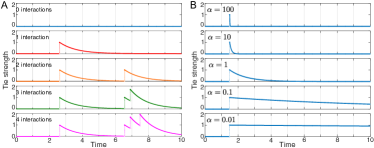
In Fig. 1A, we illustrate the evolution of the strength of a tie in our tie-decay formalism. If entities $i$ and $j$ have never interacted before time $t_{0}$, then $b_{ij}(t_{0})=0$. Suppose that they first interact at time $\tau^{\left(1\right)}>t_{0}$ (such that $a_{ij}(\tau^{\left(1\right)})=1$). Their tie strength then increases by $1$, so $b_{ij}(\tau^{\left(1\right)})=1$. It subsequently decays exponentially until they interact again, so $b_{ij}(t>\tau^{\left(1\right)})=e^{-\alpha(t-\tau^{\left(1\right)})}$ before their next interaction. If entities $i$ and $j$ next interact at time $\tau^{\left(2\right)}>\tau^{\left(1\right)}$, such that $a_{ij}(\tau^{\left(2\right)})=1$, their tie strength becomes $b_{ij}(\tau^{\left(2\right)})=e^{-\alpha(\tau^{\left(2\right)}-\tau^{\left(1\right)})}+1$, and so on.

III Eigenvector-Based Centrality Scores in Tie-Decay Networks

One common question that arises frequently when analyzing a network in scientific and industrial applications is the following: What are the most important nodes? [29] To examine this question, researchers have developed numerous centrality scores to quantify the importance of nodes according to different criteria [59].

An important family of centrality scores arise from spectral properties of the adjacency matrix (or other matrices) of a network [53, 8, 66, 75]. One attractive feature of computing centrality scores using a spectral method is that one can exploit the full structure of a network. By contrast, degree centrality is a simple centrality score that relies only on a network’s local structure. Eigenvector-based centrality scores have been insightful in numerous applications, and one can use efficient numerical algorithms to compute eigenvectors and singular vectors of matrices [25, 77]. Some of the most widely-used spectral centrality scores for directed networks include PageRank [63, 23] (which exploits the properties of a random walk on a network) and hub and authority scores [42] (which exploit both random-walk properties and the asymmetry of connections in directed networks).

In temporal networks, centrality scores must incorporate not only which nodes and edges are present in a network, but also when they are present [39, 64]. This makes it challenging to develop and analyze centrality measures in temporal networks. Some approaches have exploited numerical methods for dynamical systems to compute specific scores, such as a Katz centrality for temporal networks [28, 6], and others have employed aggregated or multilayer representations of temporal networks to calculate spectral centrality scores [3, 75]. However, these approaches have either been limited to a specific kind of centrality, or they have relied on the judicious aggregation of interactions into time bins. For example, an early paper [9] on centralities in temporal networks used a time bin of one day. Choosing an appropriate size for such a time bin is far from straightforward and requires deep knowledge of the system under study: overly coarse bins obfuscate temporal features, whereas bins that are too small may obscure network structures, yielding scores that may result more from noise than from signals.

Our tie-decay network formalism in equation (2) allows us to employ efficient numerical techniques to compute a variety of spectral centrality scores in our temporal networks. One can tune the decay parameter $\alpha$ (which one can also generalize to be node-specific, tie-specific, or time-dependent) to consider different time scales. A key benefit of our approach is that we can easily incorporate both new interactions and new nodes as a network evolves. In the present paper, we showcase an application using PageRank centrality, but it is also worthwhile to study other spectral centrality scores using our tie-decay formalism.

III-A Tie-Decay PageRank Centrality

PageRank centrality is a widely used (and historically important) eigenvector-based centrality score for time-independent networks [63, 59]. The PageRank score of a node in a network corresponds to its stationary distribution in a random walk with teleportation [23, 53]. In this type of random walk, a walker continues its walk from a node by following an outgoing edge with probability $\lambda\in(0,1)$ (where, in most versions, one chooses the edge with a probability that is proportional to its weight), and it ‘teleports’ to some other node in the network with probability $1-\lambda$. It is common to choose the destination node uniformly at random, but many other choices are possible [44, 23]. In the present paper, we employ uniform teleportation with $\lambda=0.85$ (which is a common choice). Let $B$ be the adjacency matrix of a weighted network with $n$ nodes, so $b_{ij}$ encodes the weight of a directed tie from node $i$ to node $j$. The $n\times 1$ vector $\bm{\pi}$ of PageRank scores, with $\bm{\pi}>0$ and $\left\|\bm{\pi}\right\|_{1}=1$, is the leading-eigenvector solution of the eigenvalue problem

$$G^{T}\bm{\pi}=\bm{\pi}\,,$$ (5)

where $G$ is the $n\times n$ rate matrix of a teleporting random walk:

$$G =\lambda\left(D^{\dagger}B+\mathbf{c}\mathbf{v}^{T}\right)+(1-\lambda)\mathbb{1}\mathbf{v}^{T}$$ (6)

$$=\lambda P+(1-\lambda)\mathbb{1}\mathbf{v}^{T}\,,$$

where $P=D^{\dagger}B+\mathbf{c}\mathbf{v}^{T}$; the matrix $D$ is the diagonal matrix of weighted out-degrees, so $d_{ii}=\sum_{k}b_{ik}$ and $d_{ij}=0$ when $i\neq j$; and $D^{\dagger}$ is its Moore–Penrose pseudo-inverse. The $n\times 1$ vector $\mathbf{c}$ is an indicator of ‘dangling nodes’ (i.e., nodes with $0$ out-degree): $c_{i}=1-d^{\dagger}_{ii}\sum_{k}b_{ik}$, so $c_{i}=1$ if the out-degree of $i$ is $0$ and $c_{i}=0$ otherwise. Additionally, $\mathbb{1}$ is the $n\times 1$ vector of $1$s, and the $n\times 1$ distribution vector $\mathbf{v}$ encodes the probabilities of each node to receive a teleported walker. In the present paper, we use $v_{i}={1}/{n}$ for all $i$.

The perturbations to $D^{\dagger}B$ from $\mathbf{v}$ and $\mathbf{c}$ ensure the ergodicity of the teleporting random walk, so the Perron–Frobenius theorem guarantees that $G^{T}$ has a unique right leading eigenvector $\bm{\pi}$ whose entries are all strictly positive. To calculate $\bm{\pi}$, one can perform a power iteration on $G^{T}$ [77], but in practice we do not need to explicitly construct $G^{T}$. The iteration

$$\bm{\pi}^{\left(k+1\right)}=\lambda P^{T}\bm{\pi}^{\left(k\right)}+(1-\lambda)\mathbf{v}\,,$$ (7)

with $\bm{\pi}^{\left(0\right)}=\mathbf{\left(0\right)}$ or $\bm{\pi}^{\left(0\right)}=\mathbf{v}$, converges to $\bm{\pi}$ and preserves the sparsity of $P$. This choice, which ensures that computations are efficient, is equivalent to a power iteration [23].

To compute time-dependent PageRank scores from the tie-strength matrix $B(t)$, we define the temporal transition matrix

$$P(t)=D^{\dagger}(t)B(t)+\mathbf{c}(t)\mathbf{v}^{T}\,,$$ (8)

where $D(t)$ is the diagonal matrix of weighted out-degrees (i.e., the row sums of $B(t)$) at time $t$. The rank-$1$ correction $\mathbf{c}(t)\mathbf{v}^{T}$ depends on time, because the set of dangling nodes can change in time (though $\mathbf{v}$ remains fixed). The iteration to obtain the time-dependent vector of PageRank scores $\bm{\pi}(t)$ is now given by

$$\bm{\pi}^{\left(k+1\right)}(t)=\lambda P^{T}(t)\bm{\pi}^{\left(k\right)}(t)+(1-\lambda)\mathbf{v}\,.$$ (9)

To understand the temporal evolution of $\bm{\pi}(t)$, we begin by establishing some properties of the temporal transition matrix $P(t)$ in the following lemma.

Lemma 1.

When there are no new interactions between times $t$ and $t+\Delta t$, the entries of $A(t+\Delta t)$ are all $0$ and $P(t+\Delta t)=P(t).$ If there is a single new interaction from node $i$ to node $j$, such that $a_{ij}(t+\Delta t)=1$, then $P(t+\Delta t)=P(t)+\Delta P$, where

$$\Delta P =\frac{1}{1+e^{-\alpha\Delta t}d_{ii}(t)}\mathbf{e}_{i}\mathbf{e}_{j}^{T}$$

$$\quad-\frac{1}{d_{ii}(t)\left(1+e^{-\alpha\Delta t}d_{ii}(t)\right)}\mathbf{e}_{i}\mathbf{e}_{i}^{T}B(t)-c_{i}(t)v_{i}\mathbf{e}_{i}\mathbb{1}^{T}$$ (10)

and $\mathbf{e}_{i}$ and $\mathbf{e}_{i}$, respectively, are the $i$-th and $j$-th canonical vectors.

The first term in the right-hand side of equation (10) is a matrix whose only nonzero entry is the $(i,j)$-th term, the second term is a rescaling of the $i$-th row of $B(t)$, and the third term is the perturbation due to teleportation. An important implication of Lemma 1 is that the PageRank scores do not change when there are no new interactions, so $\bm{\pi}(t+\Delta t)=\bm{\pi}(t)$. If each node or tie has different decay rates (so that now we index $\alpha$ as $\alpha_{i}$ or $\alpha_{ij}$), then this no longer has to be the case.

When there are new interactions, the following result sets an upper bound on how much the PageRank scores can change.

Theorem 1.

Suppose that there is a single interaction between times $t$ and $t+\Delta t$ from node $i$ to node $j$, such that the change $\Delta P$ in the transition matrix satisfies equation (10). It follows that

$$\left\|\bm{\pi}(t+\Delta t)-\bm{\pi}(t)\right\|_{1}$$

$$\quad\leq\frac{2\lambda}{1-\lambda}\min\left\{\pi_{i}(t),\,\frac{1}{1+e^{-\alpha\Delta t}d_{ii}(t)}-\frac{c_{i}(t)}{2}\right\}\,.$$ (11)

We present two corollaries of Theorem 1.

Corollary 1.

If $i$ is a dangling node at time $t$, then

$$\left\|\bm{\pi}(t+\Delta t)-\bm{\pi}(t)\right\|_{1}\leq\frac{2\lambda}{1-\lambda}\min\left\{\pi_{i}(t),\frac{1}{2}\right\}\,.$$ (12)

Corollary 2.

If node $i$ has one or more outgoing edges at time $t$, then

$$\left\|\bm{\pi}(t+\Delta t)-\bm{\pi}(t)\right\|_{1}$$

$$\quad\leq\frac{2\lambda}{1-\lambda}\min\left\{\pi_{i}(t),\,\frac{1}{1+e^{-\alpha\Delta t}d_{ii}(t)}\right\}\,.$$ (13)

We give proofs of Lemma 1, Theorem 1, and Corollaries 12 and 2 in Appendix A.

III-A1 Temporal Iteration

To calculate the PageRank scores at time $t+\Delta t$, we use the iteration in equation (9) to update the PageRank vector using $\bm{\pi}(t)$ as the initial value. That is,

$$\bm{\pi}^{\left(0\right)}(t+\Delta t)=\bm{\pi}(t)\,.$$ (14)

The relative error of the computed PageRank vector at iteration $k$ is

$$\left\|e_{\mathrm{rel}}^{\left(k\right)}\right\|_{1}=\left\|\bm{\pi}(t+\Delta t)-\bm{\pi}^{\left(k\right)}(t+\Delta t)\right\|_{1}\,.$$ (15)

A result from [7] (see their Theorem 6.1) implies that $\left\|e_{\mathrm{rel}}^{\left(k\right)}\right\|_{1}\leq\lambda^{k}\left\|e_{\mathrm{rel}}^{\left(0\right)}\right\|_{1}\,$. The relation $\bm{\pi}^{\left(0\right)}(t+\Delta t)=\bm{\pi}(t)$ and Theorem 1, then imply that

$$\left\|e_{\mathrm{rel}}^{\left(k\right)}\right\|_{1}\, \leq\lambda^{k}\left\|\bm{\pi}(t+\Delta t)-\bm{\pi}(t)\right\|_{1}$$

$$\leq\frac{2\lambda^{k+1}}{1-\lambda}\min\left\{\pi_{i}(t),\,\frac{1}{1+e^{-\alpha\Delta t}d_{ii}(t)}-\frac{c_{i}(t)}{2}\right\}\,.$$ (16)

Therefore, we can select an error tolerance $\epsilon$ such that $\left\|e_{\mathrm{rel}}^{\left(k^{*}\right)}\right\|_{1}\leq\epsilon$ for some number $k^{*}$ of iterations. The value $k^{*}$ represents the maximum number of iterations that we need to have a relative error of at most $\epsilon$. We compute $k^{*}$ by calculating

$$k^{*}=\frac{\ln(\epsilon)-\ln(2)+\ln(1-\lambda)-\ln\left(\min\left\{\pi_{i}(t)\,,\,\frac{1}{1+e^{-\alpha\Delta t}d_{ii}(t)}-\frac{c_{i}(t)}{2}\right\}\right)}{\ln(\lambda)}-1\,.$$ (17)

In practice, we can instead track the residual after $k$ iterations [23]:

$$\mathbf{r}^{\left(k\right)}(t+\Delta t) =\bm{\pi}^{\left(k+1\right)}(t+\Delta t)-\bm{\pi}^{\left(k\right)}(t+\Delta t)$$

$$=(1-\lambda)\mathbf{v}-\left(I_{n}-\lambda P^{T}(t+\Delta t)\right)\bm{\pi}^{\left(k\right)}(t+\Delta t)\,.$$ (18)

We use this residual to bound the relative error,

$$\left\|\bm{\pi}(t+\Delta t)-\bm{\pi}^{\left(k\right)}(t+\Delta t)\right\|_{1} =\left\|\left(I_{n}-\lambda P^{T}(t+\Delta t)\right)^{-1}\mathbf{r}^{\left(k\right)}(t+\Delta t)\right\|_{1}$$

$$\leq\frac{1}{1-\lambda}\left\|\mathbf{r}^{\left(k\right)}(t+\Delta t)\right\|_{1}\,,$$ (19)

and we thereby monitor the convergence of the iteration. In our experiments, we always obtain $\|\bm{\pi}^{\left(k+1\right)}(t+\Delta t)-\bm{\pi}^{\left(k\right)}(t+\Delta t)\|_{l_{1}}<10^{-6}$ in two iterations or fewer (see Section V-C). See [14] for an alternative approach for approximating PageRank after adding a single edge.

IV A Synthetic Example

To illustrate some of the features of our tie-decay formalism, we construct an example that illustrates the challenges of binning interactions and how our approach can help overcome them.

Figure 2: (Color online) Schematic illustration of the interactions in our synthetic network. (See the description in the main text.) We show target nodes as pink diamonds and source nodes as blue disks. In this example, there is one target at a time, and the different nodes take turns being the target. After all source nodes interact with the current target, a new node becomes the target, and all source nodes then interact with it. This cycle keeps repeating in this temporal network, which is periodic with a period of $20$ time steps.

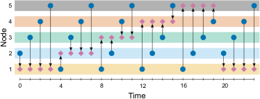
Consider a network with node set $V=\{{1,2,3,4,5}\}$. These nodes interact with each other cyclically in discrete time, with only a single edge present during each time step. At the initial time $t_{0}$, we select a ‘target node’ and a ‘source node’ and create a directed edge from the source to the target. At the next time (i.e., $t=t_{1}$), there is an edge from a different source node to the same target. This occurs with a third source node and the same target at time $t_{2}$ and with the final remaining source nodes and this target at time $t_{3}$. We have now exhausted all possible source nodes for this target, so at time $t_{4}$, we select a new target node and repeat the above process. Specifically, there is exactly one directed edge at each discrete time, and we select each of the four possible source nodes exactly once between times $t_{4}$ and $t_{7}$. We repeat this cycle thrice more, and we finish with the final source–target pair at time $t_{19}$. The process begins again at time $t_{20}$ with the first target node, and it continues periodically. In Fig. 2, we show the interactions in this synthetic temporal network for the first $25$ time steps. When we examine temporal centralities in this network, we expect its cyclical behavior to be reflected in the centrality scores of its nodes.

Figure 3: (Color online) PageRank scores over time for each node in our five-node synthetic network. (See the description in the main text.) A: Calculations of time-independent PageRank scores using sliding windows $(t_{k}-w,t_{k}]$ of different duration to aggregate interactions. B: Calculations of tie-decay PageRank scores for different values of the tie half-life.

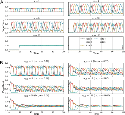
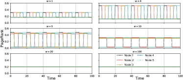
One way to examine temporal centralities of the nodes in our synthetic network is by aggregating the interactions into discrete sliding windows of duration $w$ [65, 70]. To do this, we construct time-independent networks with interactions in the time window $(t_{k}-w,t_{k}]$, and we then compute the PageRank scores of the nodes for each of these networks. In Fig. 3A, we show the PageRank scores for these networks using windows of different length. To use this approach, we require at least $w$ time steps before we can construct the first window; this is a potential issue for some investigations. Additionally, the PageRank scores are sensitive to the value of $w$. This is another potential difficulty, especially because one does not know appropriate window lengths in advance in many situations. An alternative to aggregating interactions into discrete sliding windows is to use adjacent windows of length $w$ [10] With this choice, we aggregate interactions exactly once every $w$ time steps. We show the resulting time series of PageRank scores in Fig. 10 in Appendix A-C.

When a window includes individual interactions only ($w=1$) or matches one cycle duration ($w=4$), the PageRank centrality scores capture the sequence of interactions between the nodes. We show these two cases in the top row of Fig. 3A. However, even those choices of $w$ are not without issues. Using $w=1$ neglects important temporal features, and selecting $w=4$ (the cycle length) and placing it correctly requires prior knowledge of the temporal network, which we possess only because we invented the rules to create this network. The extreme sensitivity of PageRank scores to the value of $w$ also causes other problems. For example, when $w$ is a multiple of the number of nodes and the period (e.g., $w=20$), this approach fails to give any useful information at all, because all differences in the interaction patterns are masked entirely by the window.

Figure 4: (Color online) A: Pearson correlation matrix of the PageRank time series of node $1$ in our synthetic network using sliding windows $(t_{k}-w,t_{k}]$ for $w\in\{1,\ldots,100\}$. B: Pearson correlation matrix of the tie-decay PageRank time series of node $1$ for integer half-lives $\eta_{1/2}\in\{1,\ldots,100\}$.

We now use our tie-decay formalism to obtain PageRank time series for different tie half-lives (see Fig. 3B). The cyclical dynamics of the interactions manifest in all values of the half-life $\eta_{1/2}$. Different values of $\eta_{1/2}$ entail different oscillation magnitudes, but the time series includes oscillations for all choices of $\eta_{1/2}$. Every four time steps, we observe an increase in the PageRank score of the newly-selected target node. Using our tie-decay framework also does not have the problem of ‘masking’ of the dynamics that we illustrated above.

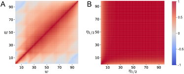
We also examine the sensitivity with respect to the choice of window length and half-life by computing the Pearson correlation of the PageRank time series for different values of $w$ and $\tau$ (for ordinary PageRank) and $\eta_{1/2}$ (for tie-decay PageRank). In Fig. 4A, we show the Pearson correlation between the time series of the (ordinary) PageRank centrality of node $1$ for each $w\in\{1,2,\ldots,100\}$. As the figure shows, binning interactions over time produces a time series that is very sensitive to the choice of $w$. The mean correlation between time series is $0.414$, and the standard deviation is $0.301$. Some time series are even correlated negatively with each other. The correlations also depend on the periodicity of our temporal network. For example, choices of $w$ for the two time series that differ by exactly $20$ have larger positive correlations with each other than with other window lengths. By comparison, the Pearson correlations between the PageRank time series in the tie-decay networks for a variety of values of the half-life $\eta_{1/2}$ (see Fig. 4B) paint a very different picture. We observe large positive correlations for many pairs of values of $\tau$. The mean correlation between the time series in $0.945$, which is much larger than what we observed for our calculation with sliding windows, and the standard deviation of $0.109$ is much smaller.

Our synthetic example of a temporal network highlights some of the advantages of our continuous-time tie-decay network formalism for temporal networks. Results from frameworks that require binning interactions can be extremely sensitive both to the choice of window length and to the placement of windows. By contrast, our tie-decay framework is more robust to parameter choices. Varying $\eta_{1/2}$ (or, equivalently, $\alpha$) adjusts the longevity of ties while maintaining similar PageRank centrality trajectories, lending confidence to investigations even when (as is usually the case) one does not possess precise knowledge of the time scales of the interactions in a system.

V The National Health Service (NHS) Retweet Network

We now compute tie-decay PageRank scores to track the evolution of node importances over time in a large data set of time-annotated interactions on Twitter.

Twitter is a social-media platform that has become a prominent channel for organizations, individuals, ‘bots’, ‘sockpuppets’, and other types of accounts to broadcast events, share ideas, report events, and socialize by posting messages (i.e., ‘tweets’) of at most 140 characters in length [43]. (Twitter subsequently expanded the maximum tweet length to 280 characters, but the maximum was 140 characters at the time that our data set was collected.) Data from Twitter has allowed researchers to study patterns and trends in a plethora of large-scale political and social events and processes, such as protests and civil unrest, public health, and information propagation [2, 3, 15, 21, 26, 56, 62, 76].

Twitter accounts (which can represent an individual, an organization, a bot, and so on) can interact in several ways, and there are various ways to encode such interactions in the form of a network. For example, accounts can subscribe to receive other accounts’ tweets (a ‘follow’ connection), can mention each other in a tweet (a ‘mention’ connection), can spread a tweet that was posted originally by someone else (a ‘retweet’ connection) to their followers, and so on. These interactions represent an explicit declaration of interest from a source account about a target, and one can thus encode them using directed networks [2]. Because these interactions are time-resolved, it is sensible to analyze Twitter networks as time-dependent networks [3].

Figure 5: Number of daily retweets among the 10,000 most-active Twitter accounts in the NHS data set.

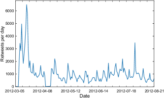
We study a retweet network, which we construct from a data set of tweets about the United Kingdom’s National Health Service (NHS) that were posted after the controversial Health and Social Care Act of 2012 [48]. Our data set covers over five months of time and includes tweets in English that include the term ‘NHS’. Specifically, we consider retweets by the 10,000 most-active Twitter accounts (according to the number of tweets in our data set) from 5 March 2012 through 21 August 2012 (see Fig. 5). All data were collected by Sinnia, a data-analytics company, using Twitter Gnip PowerTrack API. From these data, we construct a tie-decay temporal network in which the interactions are retweets. Our code for constructing tie-decay networks is available at https://bitbucket.org/walid0925/tiedecay/.

V-A Tie-Decay PageRank Centrality in the NHS Retweet Network

The temporal network of retweets from the NHS data has the tie-strength matrix $\mathbf{B}(t)$ (see equation (3)) and starts from the initial condition $\mathbf{B}(0)=0$. We construct three tie-decay networks: ones whose values of $\alpha$ correspond to tie half-lives of $1$ hour, $1$ day, and $1$ week. We compute tie-decay PageRank scores of all Twitter accounts for each of these networks.

Figure 6: (Color online) The top Twitter accounts, according to tie-decay PageRank, in the temporal NHS retweet network with three values of tie half-life. Each color is associated with a unique Twitter account, and the alternating gray and white background color indicates intervals in which the same account has the top tie-decay PageRank score. Transitions in color (from white to gray, and vice versa) indicate when there is a change in which account has the top score. The first dashed red vertical line indicates the time that @DrEoinClarke posted the tweet in the associated box; the second such line corresponds to a tweet by @marcuschown.

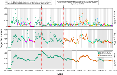
In Fig. 6, we show an example of the effect of the value of $\alpha$ on PageRank scores. We compute tie-decay PageRank scores for networks in which the tie half-life is $1$ hour, $1$ day, and $1$ week. In each panel of Fig. 6, we plot the Twitter account with the largest PageRank score at every time point; the transitions between white and gray shading indicate when there is a change in which account has the top score. When the half-life is short (i.e., $\alpha$ is large), interactions produce feeble ties that die off quickly unless there are frequent and sustained interactions between the accounts. Consequently, the tie-decay PageRank scores of the Twitter accounts change wildly in time, and (as illustrated in the top panel in Fig. 6) such a short half-life implies that the Twitter account with the top tie-decay PageRank score changes frequently. When the half-life is longer (e.g., $1$ day), ties are better able to build momentum and strengthen from interactions that otherwise would be too far apart in time. The ability to build and maintain ties results in fewer transitions between which Twitter account has the top spot in the ranking. The middle panel in Fig. 6 illustrates that we indeed observe less-frequent transitions when the half-life is $1$ day. Finally, when the half-life of a tie is $1$ week, two specific accounts (@DrEoinClarke and @marcuschown) dominate the ranking; they alternate between the top and second spots.

In this case study, we reveal two accounts as dominant ones as we tune the half-life of ties to larger values. The first of these, Eoin Clarke (@DrEoinClarke), is a Labour-party activist and was an outspoken critic of the UK coalition government’s stance in 2012 on the NHS. Marcus Chown (@marcuschown) is a science writer, journalist, and broadcaster who was also an outspoken critic of the UK government’s NHS policy in 2012. Their dominance becomes apparent as we increase the half-life of the ties. On 29 April, @DrEoinClarke posted a tweet that gathered significant attention. This tweet yields a short-lived boost in his PageRank score when $\eta_{1/2}$ is $1$ hour and $1$ day, and it yields a more sustained increase when $\eta_{1/2}$ is $1$ week. On 4 June, @marcuschown posted a tweet that boosts his PageRank score. When $\eta_{1/2}$ is $1$ day, the number of retweets of this tweet are enough to carry him to the top spot. However, when $\eta_{1/2}$ is $1$ week, the retweets are not enough to overtake @DrEoinClarke, whose ties remain strong.

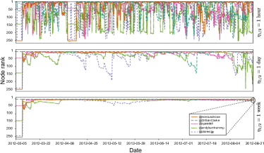
In Fig. 7, we show a complementary illustration of the effect of half-life value on the time-resolved PageRank rankings of Twitter accounts. We construct a time-independent network in which we aggregate all of the interactions in our data set — specifically, we consider $B(t)$ for $\alpha=0$ with the time $t$ set to be 21 August 2012 — and we determine the top-5 accounts by calculating the standard time-independent version of PageRank (with $\lambda=0.85$) on this network. We then track the time-dependent PageRank ranks (where rank $1$ is the Twitter account with the largest tie-decay PageRank score, and so on) of these five accounts for different values of $\alpha$ (or, equivalently, of $\eta_{1/2}$). When $\eta_{1/2}$ is $1$ hour, these accounts often overtake each other in the rankings, and the changes in rankings can be rather drastic, as some Twitter accounts drop or rise by almost $250$ spots. As we consider progressively longer half-lives, we observe less volatility in the rankings.

The experiments in Figs. 6 and 7 demonstrate how one can use $\alpha$ as a tuning parameter to reflect the longevity of relationship values in a temporal network. They also demonstrate the value of our tie-decay formalism for illustrating fluctuations in network structures. When analyzing networks in discrete time, there is a risk that aggregating interactions may conceal intermediate dynamics and nuances of network structure [18]. By contrast, our continuous-time network formalism avoids arbitrary cutoff choices (and potential ensuing biases [41]) when choosing the borders of time windows. It also allows a smoother exploration of network structure at a level of temporal granularity that is encoded in the value of $\alpha$.

Figure 7: (Color online) Time series of time-resolved ranks of five prominent Twitter accounts for aggregations of tie-decay networks with three different values of the half-life. More-important accounts are higher on the vertical axis.

V-B Aggregating Interactions versus Examining Tie-Decay Networks

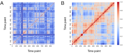
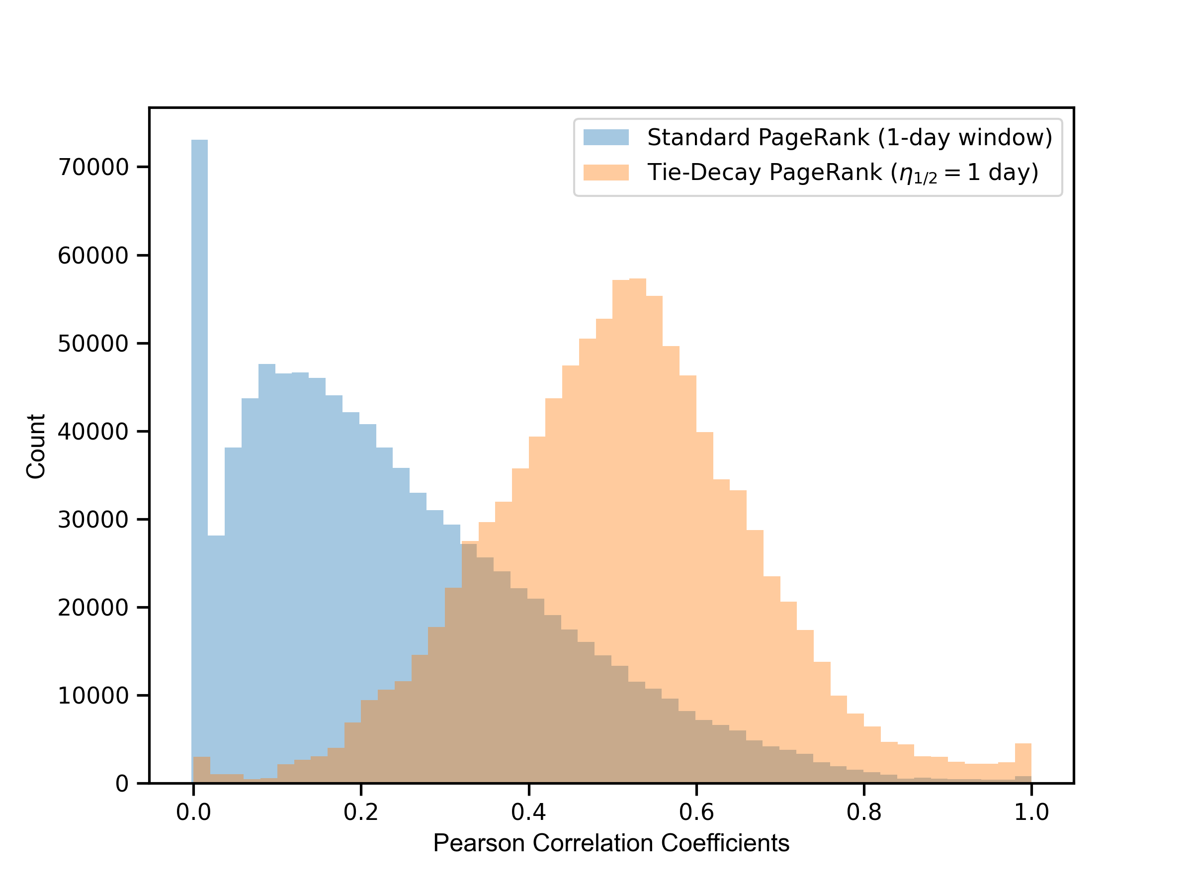
Using tie-decay networks instead of aggregating interactions via sliding windows can have a large impact on the qualitative results of an investigation. To illustrate this using the NHS data, we compare the Pearson correlation between the PageRank vectors from tie-decay networks to the Pearson correlation on networks that we construct using sliding windows. We sample $K$ equally-spaced time points between the first and last interactions in the data. At each time point $t_{k}$, we construct a time-independent network with interactions in the time window $(t_{k}-w,t_{k}]$ for a given window length $w$, and we compute the PageRank vector for this network. In Figure 8A, we show the Pearson correlation matrices between PageRank vectors using $K=1,000$ and $w=1$ day. The sampled time points are approximately four hours apart, so consecutive time points have overlapping windows. However, the Pearson correlations between the PageRank vectors from the different time-independent networks are relatively small. This is usually the case even for the PageRank vectors from time points that are near each other. Such small temporal correlations are not surprising; previous research [9] has reported that the connections in networks that one constructs by aggregating interactions on different days can vary drastically. When this occurs, the most central nodes in networks from different days can also differ drastically.

We also calculate the tie-decay PageRank vectors using the same time points. In this case, we observe a pronounced “block structure” in the correlation matrix (see Fig. 8B). That is, PageRank vectors from time points that are close to each other have large correlations with each other because tie strengths of past interactions persist in time. We can adjust the extent of such persistence by varying the half-life. In Figure 12 in Appendix A-E, we show the distributions of pairwise correlation values using both approaches.

Figure 8: (Color online) A: Pearson correlations between PageRank vectors in networks that we construct using sliding windows of $w=1~{}\text{day}$. B: Pearson correlations in tie-decay networks with $\eta_{1/2}=1~{}\text{ day}$.

V-C Computational Efficiency

In applications (e.g., for streaming data), it is often desirable to update the values of time-dependent centrality measures, such as tie-decay PageRank scores, each time that there is a new interaction. We know from Theorem 1 that there is a bound on the magnitude of the difference between the PageRank vectors at times $t$ and $t+\Delta t$ when there is a new interaction. Consequently, we expect to obtain faster convergence of the iteration for $t+\Delta t$ when we use the PageRank vector from $t$ as our initial vector than if we start the computation from scratch. To demonstrate this, we select a period of time with high activity in our NHS data — 08:00 am to 12:00 pm on 18 March 2012 (see Fig. 5) — and calculate the tie-decay PageRank vector at time $t+\Delta t$ with two different starting vectors: the uniform vector $\bm{\pi}^{\left(0\right)}(t+\Delta t)=\frac{1}{n}\mathbb{1}$ and the previous PageRank vector $\bm{\pi}^{\left(0\right)}(t+\Delta t)=\bm{\pi}(t)$. In time-independent networks, it has been observed that the uniform vector has better convergence properties than any other starting vector, in the absence of prior knowledge about the final PageRank vector [23]. In our tie-decay network formalism, given the bound between the magnitudes of the PageRank vectors at times $t$ and $t+\Delta t$, it is intuitive that using the vector from the previous time has computational advantages over other choices. We demonstrate this fact in Fig. 9.

Figure 9: (Color online) A: Cumulative number of iterations to convergence (where we define ‘convergence’ as $\|\bm{\pi}^{\left(k+1\right)}(t+\Delta t)-\bm{\pi}^{\left(k\right)}(t+\Delta t)\|_{l_{1}}<10^{-6}$) for calculating tie-decay PageRank on the NHS tweet network when the starting vector is the uniform vector (solid blue curve) and the previous PageRank vector (dashed green curve). For context, we also include the aggregate number of interactions in the network (dash–dotted orange curve) and label it on the right vertical axis. B: When analyzing the NHS network, we observe that tie-decay PageRank requires at most $2$ iterations to converge when we start from the previous time step’s PageRank vector, whereas using the uniform vector requires $7$ or more iterations. In this example, the half-life of a tie is $1$ day.

VI Conclusions and Discussion

We have introduced a continuous-time framework that incorporates tie decays for studying temporal networks, and we used our formalism — which we call ‘tie-decay networks’ — to generalize PageRank centrality to continuous time.

In our proposed tie-decay formalism, a tie between two nodes strengthens through repeated interactions and it decays in their absence. Such tie-decay networks allow one to tractably analyze time-dependent interactions without having to aggregate interactions into time windows (i.e., bins), as is typically done in existing frameworks for studying temporal networks [32, 34]. We purposely avoided aggregating interactions using time bins, whose sizes and placement are difficult to determine, by modeling the weakening of ties in time as exponentially decaying with a rate of $\alpha$ (or, equivalently, with a half-life of $\eta_{1/2}$). In addition to representing the decay of human relationships [11], as we have done in this paper, it is also possible to use our formalism more generally to model the decreasing value of old information, decay in other types of interactions, and so on.

We showcased our tie-decay formalism on both a synthetic temporal network and a network of retweets on Twitter. Our computations illustrated that adjusting the value of the half-life $\eta_{1/2}$ allows one to examine the temporal dynamics of rankings at different time scales of interest. Our examination of a synthetic network illustrated that using tie-decay networks can help mitigate serious issues that can arise form binning interactions, such as sensitivity to time scales and the masking of interaction patterns. To provide a case study for the study of tie-decay PageRank centralities in an empirical temporal network, we investigated the temporal evolution of the ranks of important accounts in a large collection of retweets about the UK’s National Health Service. We also developed a numerical scheme and bounds on the change of tie-decay PageRank scores upon the arrival of each new interaction. Such bounds are important for studying data streams, in which new data arrives at a potentially alarming rate. By tuning the decay rate of interactions, we illustrated that PageRank scores can change much more drastically when the half-life is short than when the half-life is long.

Our tie-decay formalism for continuous-time changes in network architecture provides an important step for the study of streaming network data and the development of tools to analyze temporal networks in real time. Streaming data is ubiquitous — it arises in social-media data, sensor streams, communication networks, and more [20, 45] — and analyzing tie-decay networks offers a promising approach for studying it. In the present paper, we illustrated how to perform an update of tie-decay PageRank from one time step to another, and it will be important to develop such ideas further for other types of computations (such as community detection and other types of clustering). In the short term, it will be useful to implement efficient schemes for numerical computations of tie-decay generalizations of other centralities scores (such as hubs and authorities) that are defined from eigenvectors. For instance, our framework permits a tie-decay generalization of personalized PageRank [23, 36] (by making a different choice of $\mathbf{v}$ in equation (9)), which one can use in turn to develop new, principled methods for studying local community structure in networks that evolve in continuous time. Our tie-decay formalism is also very well-suited to incorporating time-dependent strategies for teleportation in PageRank [24]. An extension of our tie-decay formalism to noninstantaneous interactions (i.e., taking durations into account) is possible by replacing the term with the Dirac $\delta$ function in equation (1) with a function that is nonzero only when a tie exists. For example, if an interaction lasts from $\tau_{\mathrm{begin}}$ until $\tau_{\mathrm{end}}$, then $H(t-\tau_{\mathrm{begin}})-H(t-\tau_{\mathrm{end}})$, where $H$ is the Heaviside step function. One can also formulate interactions with time durations using window functions [82] or test functions [35].

A wealth of other avenues are also worth pursuing. For example, it is desirable to systematically investigate heterogeneous decay rates (e.g., individual rates for nodes or ties), fit the decay parameter to data, use decay functions other than exponential ones [22, 84],, develop clustering methods for tie-decay networks, analyze localization phenomena (and their impact on centralities and clustering) [51, 75], develop and study random-network null models for tie-decay networks, incorporate noninstantaneous interactions, investigate change-point detection, and examine continuous-time networks with multiplex interactions. It is also desirable to study a variety of dynamical processes — such as contagion spread and opinion dynamics — on tie-decay networks.

Many empirical networks and data sets from which one can construct networks are time-dependent, and it is important to be able to model such systems in continuous time. Tie-decay networks offer a promising approach for further development of continuous-time temporal networks.

Appendix A Proofs

A-A Proof of Lemma 1

Proof.

When there is a new interaction from node $i$ to node $j$, the rows of $P(t+\Delta t)$ that correspond to nodes $k\neq i$ (i.e., nodes from which the new connection does not originate) are unchanged: $p_{kh}(t+\Delta t)=p_{kh}(t)$ for all $h\in\{1,\ldots,n\}$.

To determine the change in the $i$-th row of $P(t+\Delta t)$, we first examine the $i$-th row of $B(t+\Delta t)$ by calculating

$$b_{ih}(t+\Delta t)=\begin{cases}e^{-\alpha\Delta t}b_{ih}(t)\,,\qquad&h\neq j\\ e^{-\alpha\Delta t}b_{ij}(t)+1\,,\qquad&h=j\,.\end{cases}$$ (20)

We then consider the change to the rank-$1$ correction $\mathbf{c}(t)\mathbf{v}^{T}$. If $i$ is not a dangling node at time $t$, then $\mathbf{c}(t+\Delta t)=\mathbf{c}(t)$. However, if $i$ is a dangling node at time $t$, then $c_{i}(t)=1$ and $c_{i}(t+\Delta t)=0$. Therefore,

$$c_{i}(t+\Delta t)-c_{i}(t)=\begin{cases}0\,,\quad&c_{i}(t)=0\\ -1\,,\qquad&c_{i}(t)=1\,.\end{cases}$$ (21)

Observe that $c_{i}(t+\Delta t)$ necessarily equals $0$ and that $c_{i}(t)\in\{0,1\}$. Therefore,

$$c_{i}(t+\Delta t)-c_{i}(t)=-c_{i}(t)\,,$$ (22)

so the change to the correction term is

$$c_{i}(t+\Delta t)v_{i}-c_{i}(t)v_{i}=-c_{i}(t)v_{i}\,.$$ (23)

The $i$-th row of $P(t+\Delta t)$ is

$$p_{ih}(t+\Delta t)=\begin{cases}\dfrac{e^{-\alpha\Delta t}b_{ih}(t)}{1+e^{-\alpha\Delta t}\sum_{k}b_{ik}(t)}-c_{i}(t)v_{i}\,,\qquad&h\neq j\\ \\ \dfrac{e^{-\alpha\Delta t}b_{ij}(t)+1}{1+e^{-\alpha\Delta t}\sum_{k}b_{ik}(t)}-c_{i}(t)v_{i}\,,\qquad&h=j\,.\end{cases}$$ (24)

For $h\neq j$, the difference between $p_{ih}(t+\Delta t)$ and $p_{ih}(t)$ is

$$p_{ih}(t+\Delta t)-p_{ih}(t) =\frac{e^{-\alpha\Delta t}b_{ih}(t)}{1+e^{-\alpha\Delta t}\sum_{k}b_{ik}(t)}-\frac{b_{ih}(t)}{\sum_{k}b_{ik}(t)}-c_{i}(t)v_{i}$$

$$=\frac{-b_{ih}(t)}{\sum_{k}b_{ik}(t)\left[1+e^{-\alpha\Delta t}\sum_{k}b_{ik}(t)\right]}-c_{i}(t)v_{i}$$

$$=\frac{-b_{ih}(t)}{d_{ii}(t)\left[1+e^{-\alpha\Delta t}d_{ii}(t)\right]}-c_{i}(t)v_{i}\,.$$ (25)

When $h=j$, we have

$$p_{ij}(t+\Delta t)-p_{ij}(t) =\frac{1+e^{-\alpha\Delta t}b_{ij}(t)}{1+e^{-\alpha\Delta t}\sum_{k}b_{ik}(t)}-\frac{b_{ij}(t)}{\sum_{k}b_{ik}(t)}-c_{i}(t)v_{i}$$

$$=\frac{\sum_{k}b_{ik}(t)-b_{ij}(t)}{\sum_{k}b_{ik}(t)\left[1+e^{-\alpha\Delta t}\sum_{k}b_{ik}(t)\right]}-c_{i}(t)v_{i}$$

$$=\frac{d_{ii}(t)-b_{ij}(t)}{d_{ii}(t)\left[1+e^{-\alpha\Delta t}d_{ii}(t)\right]}-c_{i}(t)v_{i}$$

$$=\frac{1}{1+e^{-\alpha\Delta t}d_{ii}(t)}-\frac{b_{ij}(t)}{d_{ii}(t)\left[1+e^{-\alpha\Delta t}d_{ii}(t)\right]}-c_{i}(t)v_{i}\,.$$ (26)

In matrix terms, the change from $P(t)$ to $P(t+\Delta t)$ is thus

$$\Delta P =\frac{1}{1+e^{-\alpha\Delta t}d_{ii}(t)}\mathbf{e}_{i}\mathbf{e}_{j}^{T}$$

$$\quad-\frac{1}{d_{ii}(t)\left(1+e^{-\alpha\Delta t}d_{ii}(t)\right)}\mathbf{e}_{i}\mathbf{e}_{i}^{T}B(t)-c_{i}(t)v_{i}\mathbf{e}_{i}\mathbb{1}^{T}\,,$$ (27)

which concludes the proof. ∎

A-B Proof of Theorem 1

Proof.

The change in PageRank scores with one new interaction is

$$\bm{\pi}(t+\Delta t)-\bm{\pi}(t) =\left[\lambda(P(t)^{T}+\Delta P^{T})+(1-\lambda)\mathbf{v}\mathbb{1}^{T}\right]\bm{\pi}(t+\Delta t)$$

$$\quad-\left[\lambda P(t)^{T}+(1-\lambda)\mathbf{v}\mathbb{1}^{T}\right]\bm{\pi}(t)$$ (28)

$$=\lambda P(t)^{T}(\bm{\pi}(t+\Delta t)-\bm{\pi}(t))+\lambda\Delta P^{T}\bm{\pi}(t+\Delta t)\,.$$

Rearranging terms gives

$$\left(I_{n}-\lambda P(t)^{T}\right)\left(\bm{\pi}(t+\Delta t)-\bm{\pi}(t)\right)=\lambda\Delta{P}^{T}\bm{\pi}(t+\Delta t)\,,$$ (29)

which implies that

$$\bm{\pi}(t+\Delta t)-\bm{\pi}(t)=\lambda\left(I_{n}-\lambda P(t)^{T}\right)^{-1}\Delta P^{T}\bm{\pi}(t+\Delta t)\,,$$ (30)

where $I_{n}$ is the $n\times n$ identity matrix. From a Neumann-series expansion [78], we see that $\left\|(I_{n}-\lambda P(t)^{T})^{-1}\right\|_{1}$ is bounded above by $1/(1-\lambda)$.

Taking norms on both sides of (30) yields

$$\left\|\bm{\pi}(t+\Delta t)-\bm{\pi}(t)\right\|_{1}\leq\frac{\lambda}{1-\lambda}\left\|\Delta P^{T}\right\|_{1}\,.$$ (31)

Noting that $\left\|\Delta P^{T}\right\|_{1}=\left\|\Delta P\right\|_{\infty}$, we use the definition of $\Delta P$ from equation (10) to obtain

$$\begin{split}\left\|\bm{\pi}(t+\Delta t)-\bm{\pi}(t)\right\|_{1}\leq&\frac{\lambda}{(1-\lambda)(1+e^{-\alpha\Delta t}d_{ii}(t))}\left\|\mathbf{e}_{i}\mathbf{e}_{j}^{T}-\frac{1}{d_{ii}(t)}\mathbf{e}_{i}\mathbf{e}_{i}^{T}B(t)\right\|_{\infty}\\ &-\frac{\lambda c_{i}(t)v_{i}}{1-\lambda}\left\|\mathbf{e}_{i}\mathbb{1}^{T}\right\|_{\infty}\,.\end{split}$$ (32)

Recall that $B(t)$ is the tie-strength matrix and that $\mathbf{e}_{i}$ and $\mathbf{e}_{j}$, respectively, are the $i$-th and $j$-th canonical vectors. Let $Q=\mathbf{e}_{i}\mathbf{e}_{j}^{T}-\frac{1}{d_{ii}(t)}\mathbf{e}_{i}\mathbf{e}_{i}^{T}B(t)$ be the matrix with elements

$$q_{hk}=\begin{cases}1-b_{hk}(t)/d_{ii}(t)\,,&\qquad h=i\,,k=j\\ -b_{hk}(t)/d_{ii}(t)\,,&\qquad h=i\,,k\neq j\\ 0\,,&\qquad\text{otherwise}\,,\end{cases}$$ (33)

so $Q$ has nonzero elements only in row $i$. Noting that $d_{ii}(t)=\sum_{k}b_{ik}(t)$ and using

$$\left\|Q\right\|_{\infty}=\max_{1\leq h\leq n}\sum_{k=1}^{n}|q_{hk}|=\sum_{k=1}^{n}|q_{ik}|\,,$$ (34)

we see that

$$\left\|Q\right\|_{\infty}\leq 2\,.$$ (35)

We also observe that $\mathbf{e}_{i}\mathbb{1}^{T}$ is the $n\times n$ matrix whose elements are equal to $1$ in row $i$ and are equal to $0$ elsewhere. Therefore,

$$\left\|\mathbf{e}_{i}\mathbb{1}^{T}\right\|_{\infty}=n\,.$$ (36)

With $nv_{i}=1$ (i.e., uniform teleportation), it follows from equations (32), (35), and (36) that

$$\left\|\bm{\pi}(t+\Delta t)-\bm{\pi}(t)\right\|_{1}\leq\frac{2\lambda}{(1-\lambda)(1+e^{-\alpha\Delta t}d_{ii}(t))}-\frac{\lambda c_{i}(t)}{1-\lambda}\,.$$ (37)

The change in the PageRank vector is also subject to the bound [47, 60]

$$\left\|\bm{\pi}(t+\Delta t)-\bm{\pi}(t)\right\|_{1}\leq\frac{2\lambda}{1-\lambda}\sum_{s\in\mathcal{S}(t+\Delta t)}\pi_{s}(t)=\frac{2\lambda}{1-\lambda}\pi_{i}(t)\,,$$ (38)

where $\mathcal{S}(t+\Delta t)$ is the set of nodes (in this case, just node $i$) that experience a change in transition probabilities (i.e., a change in out-edges). Combining the bounds in (37) and (38) yields

$$\left\|\bm{\pi}(t+\Delta t)-\bm{\pi}(t)\right\|_{1}\leq\frac{2\lambda}{1-\lambda}\min\left\{\pi_{i}(t),\,\frac{1}{1+e^{-\alpha\Delta t}d_{ii}(t)}-\frac{c_{i}(t)}{2}\right\}\,,$$ (39)

which completes our proof. ∎

Note that $d_{ii}(t)>0\iff c_{i}(t)=0$ and $d_{ii}(t)=0\iff c_{i}(t)=1$, which guarantees that the quantity on the right-hand side of (39) is always positive. This gives the results in Corollaries 12 and 2.

A-C Synthetic Network: Using Adjacent Time Windows

In our synthetic network from Section IV, suppose that we aggregate the interactions into adjacent (i.e., non-overlapping) windows of length $w$. We then calculate PageRank time series for the resulting sequence of time-independent networks and show our results in Fig. 10.

Figure 10: (Color online) PageRank scores over time for each node in our synthetic example using adjacent time windows.

A-D NHS Retweet Network: Network Statistics

—

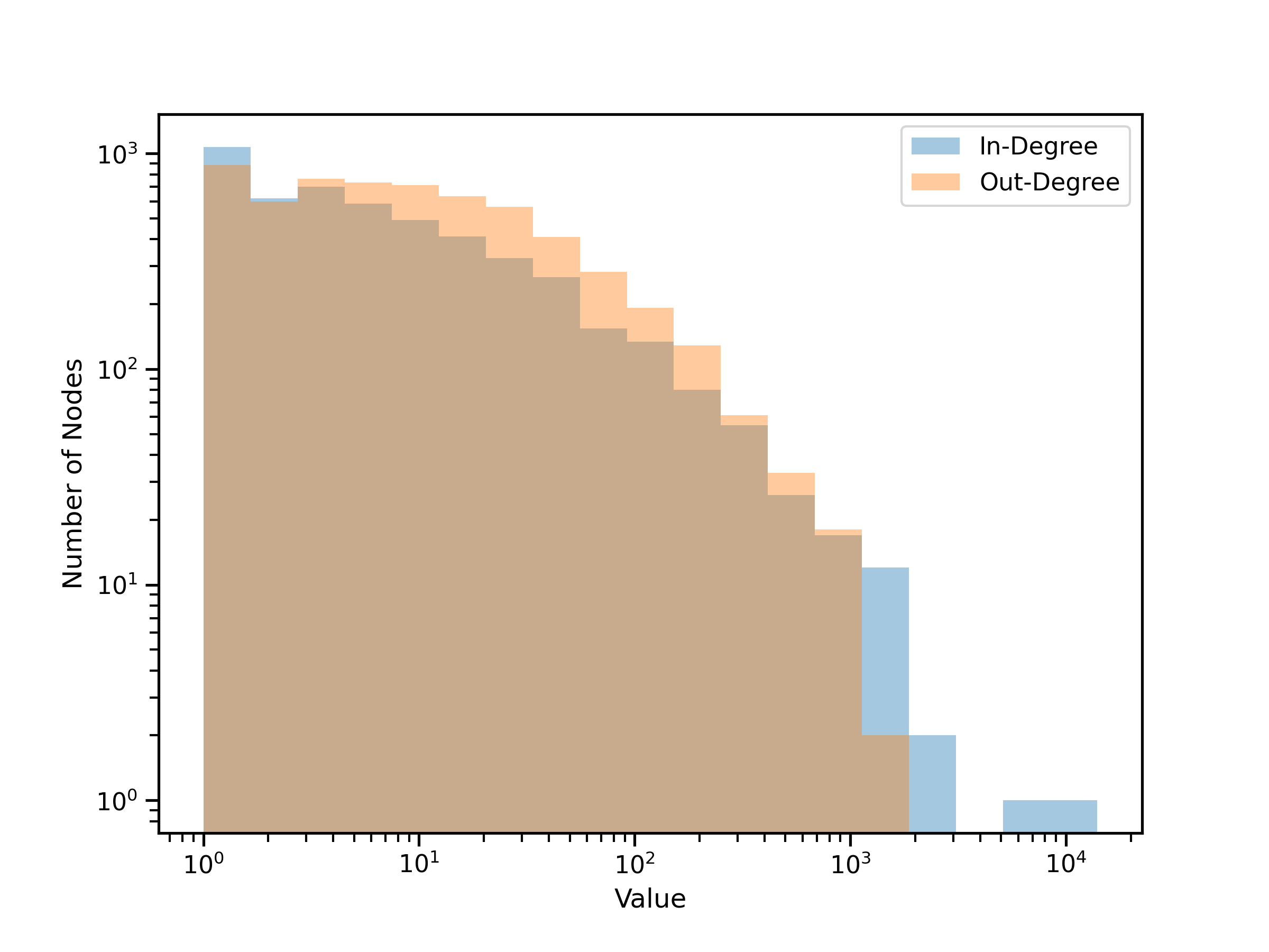
The NHS network includes retweets between the 10,000 most-active accounts, where we measure their activity as their number of tweets in the data set. There are 181,123 retweets between the 10,000 most active accounts between 5 March 2012 and 21 August 2012. We interpret each of these retweets as one interaction. In total, 6,866 of the 10,000 accounts interact with each other via retweets at least once during this time period. There are 6,013 users who retweet others, and 4,957 users who have their tweets retweeted. In Fig. 11, we show the the distribution of retweets among these users.

Figure 11: (Color online) Distributions of retweets received (i.e., in-degree) and sent (i.e., out-degree) in the NHS retweet network between 5 March 2012 and 21 August 2012.

A-E NHS Retweet Network: Aggregating Interactions Versus Using Tie-Decay Networks

Figure 12: (Color online) Distributions of Pearson correlation coefficients for the correlation matrices in Fig 8. We show the distribution for the standard PageRank score with time windows of 1 day in blue and the distribution for tie-decay PageRank with a half-life of $\eta_{1/2}=1$ day in orange.

Author Biographies

Walid Ahmad received his B.Sc. in Applied Mathematics from Columbia University and his M.Sc. in Mathematical Modelling and Scientific Computing from the University of Oxford. He is currently a machine-learning research engineer at Reverie Labs, where he works on machine-learning methods for computational drug discovery.

Mason A. Porter is a professor in the Department of Mathematics at University of California, Los Angeles. His research interests are in networks, complex systems, and nonlinear systems. He is a Fellow of the American Mathematical Society, the American Physical Society, and the Society for Industrial and Applied Mathematics.

Mariano Beguerisse-Díaz is a senior research scientist at Spotify and a visiting fellow at the University of Oxford. He has held research fellowships at the University of Oxford and Imperial College London. His research interests include network science, data science, mathematical biology, recommendation systems, computational social science, and mathematical modeling.

References

- [1] M. Bazzi, M. A. Porter, S. Williams, M. McDonald, D. J. Fenn, and S. D. Howison, Community detection in temporal multilayer networks, with an application to correlation networks, Multiscale Modeling & Simulation: A SIAM Interdisciplinary Journal, 14 (2016), pp. 1–41.
- [2] M. Beguerisse-Díaz, G. Garduño Hernández, B. Vangelov, S. N. Yaliraki, and M. Barahona, Interest communities and flow roles in directed networks: The Twitter network of the UK riots., Journal of the Royal Society: Interface, 11 (2014).
- [3] M. Beguerisse-Díaz, A. K. McLennan, G. G. no Hernández, M. Barahona, and S. J. Ulijaszek, The ‘who’ and ‘what’ of #diabetes on Twitter, Digital Health, 3 (2017), p. 2055207616688841.
- [4] M. Beguerisse-Díaz, M. A. Porter, and J.-P. Onnela, Competition for popularity in bipartite networks, Chaos, 20 (2010), p. 043101.
- [5] I. V. Belykh, V. N. Belykh, and M. Hasler, Blinking model and synchronization in small-world networks with a time-varying coupling, Physica D, 195 (2004), pp. 188–206.
- [6] F. Béres, R. Pálovics, A. Oláh, and A. A. Benczúr, Temporal walk based centrality metric for graph streams, Applied Network Science, 3 (2018), p. 32.
- [7] M. Bianchini, M. Gori, and F. Scarselli, Inside PageRank, ACM Transactions on Internet Technology (TOIT), 5 (2005), pp. 92–128.
- [8] P. Bonacich and P. Lloyd, Eigenvector-like measures of centrality for asymmetric relations, Social Networks, 23 (2001), pp. 191–201.
- [9] D. Braha and Y. Bar-Yam, From centrality to temporary fame: Dynamic centrality in complex networks, Complexity, 12 (2006), pp. 59–63.
- [10] D. Braha and Y. Bar-Yam, Time-dependent complex networks: Dynamic centrality, dynamic motifs, and cycles of social interactions, in Adaptive Networks, Springer, 2009, pp. 39–50.
- [11] R. S. Burt, Decay functions, Social Networks, 22 (2000), pp. 1–28.
- [12] R. S. Caceres, T. Berger-Wolf, and R. Grossman, Temporal scale of processes in dynamic networks, in 11th International Conference on Data Mining Workshops (ICDMW), IEEE, 2011, pp. 925–932.
- [13] K. Carley, Dynamic network analysis. Dynamic social network modelling and analysis, in Workshop summary and papers, The National Academies Press, Washington, 2003.
- [14] S. Chien, C. Dwork, R. Kumar, D. R. Simon, and D. Sivakumar, Link evolution: Analysis and algorithms, Internet Mathematics, 1 (2004), pp. 277–304.
- [15] P. Cihon and T. Yasseri, A biased review of biases in Twitter studies on political collective action, Frontiers in Physics, 4 (2016), p. 34.
- [16] R. Erban, S. J. Chapman, and P. K. Maini, A practical guide to stochastic simulations of reaction–diffusion processes, arXiv:0704.1908, (2007).
- [17] J. D. Farmer, S. A. Kauffman, N. H. Packard, and A. S. Perelson, Adaptive dynamic networks as models for the immune system and autocatalytic sets, Annals of the New York Academy of Sciences, 504 (1987), pp. 118–131.
- [18] D. J. Fenn, M. A. Porter, P. Mucha, M. McDonald, S. Williams, N. F. Johnson, and N. S. Jones, Dynamical clustering of exchange rates, Quantitative Finance, 12 (2012), pp. 1493–1520.
- [19] J. Flores and M. Romance, On eigenvector-like centralities for temporal networks: Discrete vs. continuous time scales, Journal of Computational and Applied Mathematics, 330 (2018), pp. 1041–1051.
- [20] M. M. Gaber, A. Zaslavsky, and S. Krishnaswamy, Mining Data Streams: A Review, SIGMOD Rec., 34 (2005), pp. 18–26.
- [21] J. Giles, Making the links, Nature, 488 (2012), p. 448.
- [22] J. P. Gleeson, D. Cellai, J.-P. Onnela, M. A. Porter, and F. Reed-Tsochas, A simple generative model of collective online behavior, Proceedings of the National Academy of Sciences of the United States of America, 111 (2014), pp. 10411–10415.
- [23] D. F. Gleich, PageRank beyond the Web, SIAM Review, 57 (2015), pp. 321–363.
- [24] D. F. Gleich and R. A. Rossi, A dynamical system for PageRank with time-dependent teleportation, Internet Mathematics, 10 (2014), pp. 188–217.
- [25] G. H. Golub and C. F. Van Loan, Matrix Computations, Johns Hopkins Studies in the Mathematical Sciences, Johns Hopkins University Press, Baltimore, MD, 4th ed., 2012.
- [26] S. González-Bailón and N. Wang, Networked discontent: The anatomy of protest campaigns in social media, Social Networks, 44 (2016), pp. 95–104.
- [27] P. Grindrod and D. J. Higham, A Matrix Iteration for Dynamic Network Summaries, SIAM Review, 55 (2013), pp. 118–128.
- [28] P. Grindrod and D. J. Higham, A dynamical systems view of network centrality, Proceedings of the Royal Society A: Mathematical, Physical and Engineering Sciences, 470 (2014), p. 20130835.
- [29] P. Grindrod, D. J. Higham, and P. Laflin, The Graph Whisperers, Springer International Publishing, Cham, Switzerland, 2016, pp. 271–279.
- [30] N. O. Hodas and K. Lerman, How visibility and divided attention constrain social contagion, in 2012 International Conference on Privacy, Security, Risk and Trust and 2012 International Confernece on Social Computing, Sept 2012, pp. 249–257.
- [31] T. Hoffmann, M. A. Porter, and R. Lambiotte, Generalized master equations for non-Poisson dynamics on networks, Physical Review E, 86 (2012), p. 046102.
- [32] P. Holme, Modern temporal network theory: A colloquium, The European Physical Journal B, 88 (2015), p. 234.
- [33] P. Holme and J. Saramäki, Temporal networks, Physics Reports, 519 (2012), pp. 97–125.
- [34] P. Holme and J. Saramäki, eds., Temporal Network Theory, Springer International Publishing, Cham, Switzerland, 2019.
- [35] S. Howison, Practical Applied Mathematics: Modelling, Analysis, Approximation, Cambridge Series in Applied Mathematics, Cambridge University Press, 2003.
- [36] L. G. S. Jeub, P. Balachandran, M. A. Porter, P. J. Mucha, and M. W. Mahoney, Think locally, act locally: The detection of small, medium-sized, and large communities in large networks, Physical Review E, 91 (2015), p. 012821.
- [37] E. M. Jin, M. Girvan, and M. E. J. Newman, Structure of growing social networks, Physical Review E, 64 (2001), p. 046132.
- [38] L. Katz and C. H. Proctor, The concept of configuration of interpersonal relations in a group as a time-dependent stochastic process, Psychometrika, 24 (1959), pp. 317–327.
- [39] H. Kim and R. Anderson, Temporal node centrality in complex networks, Physical Review E, 85 (2012), p. 026107.
- [40] M. Kivelä, A. Arenas, M. Barthelemy, J. P. Gleeson, Y. Moreno, and M. A. Porter, Multilayer networks, Journal of Complex Networks, 2 (2014), pp. 203–271.
- [41] M. Kivelä and M. A. Porter, Estimating interevent time distributions from finite observation periods in communication networks, Physical Review E, 92 (2015), p. 052813.
- [42] J. M. Kleinberg, Authoritative sources in a hyperlinked environment, Journal of the ACM (JACM), 46 (1999), pp. 604–632.
- [43] H. Kwak, C. Lee, H. Park, and S. Moon, What is Twitter, a Social Network or a News Media?, in Proceedings of the 19th International Conference on World Wide Web, WWW ’10, New York, NY, USA, 2010, ACM, pp. 591–600.
- [44] R. Lambiotte and M. Rosvall, Ranking and clustering of nodes in networks with smart teleportation, Physical Review E, 85 (2012), p. 056107.
- [45] M. Latapy, T. Viard, and C. Magnien, Stream graphs and link streams for the modeling of interactions over time, Social Network Analysis and Mining, 8 (2018), p. 61.
- [46] P. J. Laub, T. Taimre, and P. K. Pollett, Hawkes processes, arXiv preprint arXiv:1507.02822, (2015).
- [47] H. C. Lee and A. Borodin, Perturbation of the hyper-linked environment, in International Computing and Combinatorics Conference, Springer, 2003, pp. 272–283.
- [48] legislation.gov.uk, Health and Social Care Act 2012. Available at http://www.legislation.gov.uk/ukpga/2012/7/contents/enacted/data.htm. Accessed: 2016-08-19.
- [49] K. Lerman, Information is not a virus, and other consequences of human cognitive limits, Future Internet, 8 (2016), p. 21.
- [50] K. Lerman, R. Ghosh, and T. Surachawala, Social contagion: An empirical study of information spread on Digg and Twitter follower graphs, (2012). arXiv:1202.3162.
- [51] T. Martin, X. Zhang, and M. E. J. Newman, Localization and centrality in networks, Physical Review E, 90 (2014), p. 052808.
- [52] N. Masuda and R. Lambiotte, A Guide to Temporal Networks, vol. 4 of Series on Complexity Science, World Scientific, Singapore, 2016.
- [53] N. Masuda, M. A. Porter, and R. Lambiotte, Random walks and diffusion on networks, Physics Reports, 716–717 (2017), pp. 1–58.
- [54] N. Masuda and L. Rocha, A Gillespie algorithm for non-Markovian stochastic processes, SIAM Review, 60 (2018), pp. 95–115.
- [55] R. Michalski, B. K. Szymański, P. Kazienko, C. Lebiere, O. Lizardo, and M. Kulisiewicz, Social networks through the prism of cognition, arXiv:1806.04658, (2018).
- [56] A. J. Morales, J. C. Losada, and R. M. Benito, Users structure and behavior on an online social network during a political protest, Physica A, 391 (2012), pp. 5244–5253.
- [57] S. Motegi and N. Masuda, A network-based dynamical ranking system for competitive sports, Scientific Reports, 2 (2012), p. 904.
- [58] H. Navarro, G. Miritello, A. Canales, and E. Moro, Temporal patterns behind the strength of persistent ties, European Physical Journal — Data Science, 6 (2017), p. 31.
- [59] M. E. J. Newman, Networks, Oxford University Press, Oxford, UK, second ed., 2018.
- [60] A. Y. Ng, A. X. Zheng, and M. I. Jordan, Link analysis, eigenvectors and stability, in International Joint Conference on Artificial Intelligence, vol. 17, Lawrence Erlbaum Associates LTD, 2001, pp. 903–910.
- [61] J.-P. Onnela, J. Saramäki, J. Hyvönen, G. Szabó, M. A. de Menezes, K. Kaski, A.-L. Barabási, and J. Kertész, Analysis of a large-scale weighted network of one-to-one human communication, New Journal of Physics, 9 (2007), p. 179.
- [62] D. J. P. O’Sullivan, G. Garduño-Hernández, J. P. Gleeson, and M. Beguerisse-Díaz, Integrating sentiment and social structure to determine preference alignments: The Irish Marriage Referendum, Royal Society Open Science, 4 (2017), p. 170154.
- [63] Page, L. and Brin, S. and Motwani, R. and Winograd, T., The PageRank citation ranking: Bringing order to the Web, in Proceedings of the 7th International World Wide Web Conference, 1998, pp. 161–172.
- [64] R. K. Pan and J. Saramäki, Path lengths, correlations, and centrality in temporal networks, Physical Review E, 84 (2011), p. 016105.
- [65] L. Peel and A. Clauset, Detecting change points in the large-scale structure of evolving networks, in Proceedings of the Twenty-Ninth AAAI Conference on Artificial Intelligence, AAAI ’15, AAAI Press, 2015, pp. 2914–2920.
- [66] N. Perra and S. Fortunato, Spectral centrality measures in complex networks, Physical Review E, 78 (2008), p. 036107.
- [67] M. A. Porter and J. P. Gleeson, Dynamical Systems on Networks: A Tutorial, vol. 4 of Frontiers in Applied Dynamical Systems: Reviews and Tutorials, Springer International Publishing, Cham, Switzerland, 2016.
- [68] I. Psorakis, Probabilistic Inference in Ecological Networks: Graph Discovery, Community Detection and Modelling Dynamic Sociality, PhD thesis, D.Phil. Thesis, University of Oxford, 2013.
- [69] I. Psorakis, S. J. Roberts, I. Rezek, and B. C. Sheldon, Inferring social network structure in ecological systems from spatio-temporal data streams, Journal of the Royal Society Interface, 9 (2012), pp. 3055–3066.
- [70] S. D. Ridder, B. Vandermarliere, and J. Ryckebusch, Detection and localization of change points in temporal networks with the aid of stochastic block models, Journal of Statistical Mechanics: Theory and Experiment, 2016 (2016), p. 113302.
- [71] J. Saramäki and E. Moro, From seconds to months: An overview of multi-scale dynamics of mobile telephone calls, The European Physical Journal B, 88 (2015), p. 164.
- [72] U. Sharan and J. Neville, Exploiting time-varying relationships in statistical relational models, in Proceedings of the 9th WebKDD and 1st SNA-KDD 2007 Workshop on Web Mining and Social Network Analysis, WebKDD/SNA-KDD ’07, New York, NY, USA, 2007, Association for Computing Machinery, pp. 9–15.
- [73] T. A. B. Snijders, The statistical evaluation of social network dynamics, Sociological Methodology, 31 (2001), pp. 361–395.
- [74] R. Sulo, T. Berger-Wolf, and R. Grossman, Meaningful selection of temporal resolution for dynamic networks, in Proceedings of the Eighth Workshop on Mining and Learning with Graphs, MLG ’10, New York, NY, USA, 2010, ACM, pp. 127–136.
- [75] D. Taylor, S. A. Myers, A. Clauset, M. A. Porter, and P. J. Mucha, Eigenvector-based centrality measures for temporal networks, Multiscale Modeling and Simulation: A SIAM Interdisciplinary Journal, 15 (2017), pp. 537–574.
- [76] E. Tonkin, H. D. Pfeiffer, and G. Tourte, Twitter, information sharing and the London riots?, Bulletin of the American Society for Information Science and Technology, 38 (2012), pp. 49–57.
- [77] L. N. Trefethen and D. Bau, Numerical Linear Algebra, Society for Industrial and Applied Mathematics, Philadelphia, PA, USA, 1997.
- [78] E. E. Tyrtyshnikov, A Brief Introduction to Numerical Analysis, Birkhäuser, Basel, Switzerland, 1997.
- [79] E. Valdano, M. R. Fiorentin, C. Poletto, and V. Colizza, Epidemic threshold in continuous-time evolving networks, Physical Review Letters, 120 (2018), p. 068302.
- [80] C. L. Vestergaard and M. Génois, Temporal Gillespie algorithm: Fast simulation of contagion processes on time-varying networks, PLoS Computational Biology, 11 (2015), p. e1004579.
- [81] S. Wasserman and D. Iacobucci, Sequential social network data, Psychometrika, 53 (1988), pp. 261–282.
- [82] E. W. Weisstein, CRC Concise Encyclopedia of Mathematics, Second Edition, CRC Press, Boca Raton, FL, USA, 2002.
- [83] J. T. Wixted and E. B. Ebbesen, On the form of forgetting, Psychological science, 2 (1991), pp. 409–415.
- [84] X. Yang and J. Fan, Influential user subscription on time-decaying social streams, arXiv:1802.05305, (2018).
- [85] L. Zino, A. Rizzo, and M. Porfiri, Continuous-time discrete-distribution theory for activity-driven networks, Physical Review Letters, 117 (2016), p. 228302.
- [86] L. Zino, A. Rizzo, and M. Porfiri, An analytical framework for the study of epidemic models on activity driven networks, Journal of Complex Networks, 5 (2017), pp. 924–952.