Tiling iterated function systems and Anderson-Putnam theory

Abstract.

The theory of fractal tilings of fractal blow-ups is extended to graph-directed iterated function systems, resulting in generalizations and extensions of some of the theory of Anderson and Putnam and of Bellisard et al. regarding self-similar tilings.

1. Introduction

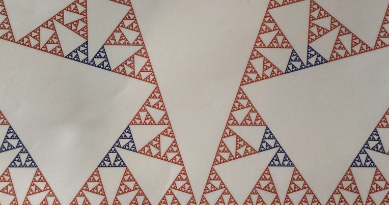
Figure 1. Illustration of part of a tiling of a fractal blow-up. There are two tiles, both topologically conjugate to Sierpinski triangles, a small blue one and a larger red one.

Given a natural number $M$, this paper is concerned with certain tilings of strict subsets of Euclidean space $\mathbb{R}^{M}$ and of $\mathbb{R}^{M}$ itself. An example of part of such a tiling is illustrated in Figure 1. We substantially generalize the theory of tilings of fractal blow-ups introduced in [10, 12] and connect the result to the standard theory of self-similar tiling [1]. The central main result in this paper is presented in Sections 7 and 8, with consequences in Section 9. In Section 7 we extend the earlier work by establishing the exact conditions under which for example translations of a tiling agree with another tiling; in Section 9 we generalize this result to tilings of blow-ups of graph directed IFS. Our other main contributions are (i) development of an algebraic and symbolic fractal tiling theory along the lines initiated by Bandt [3]; (ii) demonstration that the Smale system at the heart of Anderson-Putnam theory is conjugate to a type of symbolic dynamical system that is familiar to researchers in deterministic fractal geometry; and (iii) to show that the theory applies to tilings of fractal blow-ups, where the tiles may have no interior and the group of translations on the tilings space is replaced by a groupoid of isometries. At the foundational level, this work has notions in common with the work of Bellisard et al. [15] but we believe that our approach casts new light and simplicity upon the subject.

We construct tilings using what we call tiling iterated function systems (TIFS) defined in Section 3.3. A tiling IFS is a graph (directed) IFS [7, 13, 20] where the maps are similitudes and there is a certain algebraic constraint on the scaling ratios. When the tilings are recognizable (see [1] and references therein) or more generally the TIFS is locally rigid, defined in Section 8, the tiling space admits an invertible inflation map. Our construction of a self-similar tiling using a TIFS is illustrated in Figure 2; it is similar to the one in [10, 12], the key difference being generalization to graph IFS. In the standard theory [1] self-similar tilings of $\mathbb{R}^{M}$ are constructed by starting from a finite set of CW-complexes which, after being scaled up by a fixed factor, can be tiled by translations of members of the original set. (It is easy to see this arrangement may be described in terms of a graph IFS, that is a finite set of contractive similitudes that map the set of CW-complexes into itself, together with a directed graph that describes which maps take which complex into which.) By careful iteration of this inflation (and subdivision) process, successively larger patches and, in the limit, tilings may be obtained. We follow a similar procedure here, but our setting is more general and results in a rich symbolic understanding of (generalized) tiling spaces.

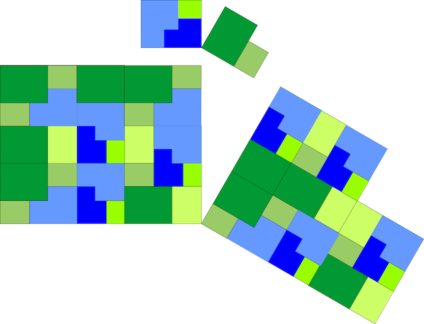
Figure 2. This figure hints at how a family of tilings may be generated using a graph directed IFS.

In [1] it is shown that inflation map acting on a space of self-similar tilings, as defined there, is conjugate to a shift acting on an inverse limit space constructed using pointed tilings, and semi-conjugate to a shift acting on a symbolic space. This raises these questions. When are two fractal tilings isometric? How can one tell symbolically if two tilings are isometric? How can one tell if two tiling dynamical systems are topologically conjugate? What is the topological structure of the tiling space and how does the tiling dynamical system act on it? For example, can one see purely symbolically the solenoid structure of the tiling space in the case of the Penrose tilings, and what happens in the case of purely fractal tilings? When the tiles are CW-compexes, an approach is via study of invariants such as zeta functions and cohomology when these can be calculated, as in [1]. Here we approach the answers by constructing symbolic representation of the (generalized) Anderson-Putnam complex and associated tiling dynamics.

In Section 2 we provide necessary notation and background regarding graph IFS and their attractors. We focus on the associated symbolic spaces, namely the code or address spaces of IFS theory, as these play a central role. Key to our main results is the relationship between the attractor $A$ of a graph IFS $\left(\mathcal{F},\mathcal{G}\right)$ and its address space $\Sigma,$ all defined in Section 2: this relationship is captured in a well-known continuous coding map $\pi:\Sigma\rightarrow A$. Sets of addresses in $\Sigma$ are mapped to points in $A$ by $\pi$. This structure is reflected in a second mapping $\Pi:\Sigma^{{\dagger}}\rightarrow\mathbb{T}$ introduced in Section 3, where $\mathbb{T}$ is the tiling space that we associate with $\left(\mathcal{F},\mathcal{G}\right)$. The important results of Section 2 are the notation introduced there, the information summarized in Theorem 1, which concerns the existence and structure of attractors, and Theorem 2 which concerns the coding map $\pi:\Sigma\rightarrow A$.

Section 3 introduces TIFS (tiling iterated function systems) and associated tiling space $\mathbb{T}$, shows the existence of a family of tilings $\{\Pi(\theta):\theta\in\Sigma^{{\dagger}}\}\subset\mathbb{T}$, and explores their relationship to what we call a canonical family of tilings $\{T_{n}^{(v)}\}$ and their symbolic counterparts, symbolic tilings, $\{\Omega_{n}^{(v)}\}$, certain subsets of $\Sigma^{{\dagger}}$. We explore the action of an invertible symbolic inflation operator that acts on the symbolic tilings and $\{\Omega_{n}^{(v)}\}$ and its inverse. When $\Pi:\Sigma^{{\dagger}}\rightarrow\mathbb{T}$ is one-to-one, which occurs when the TIFS is what we call locally rigid, there is a commutative relationship between symbolic inflation/deflation on $\{\Omega_{n}^{(v)}\}$ and inflation/deflation on the range of $\Pi$. **More to go here, then simplify.

In Sections 7 we define relative and absolute addresses of tiles in tilings: these addressing schemes for tiles in tilings ***. In Section 8 we arrive at our main result, Theorem **: we characterize members of $\mathbb{T}$ which are isometric in terms of their addresses. This in turn allows us to describe the full tiling space, obtained by letting the group of Euclidean isometries act on the range of $\Pi$. **More to go here.

**Discussion of ”forces the borders” (Anderson and Putnam), ”unique composition property” (Solomyak 1997), ”recognizability” and relation to rigid.

2. Attractors of graph directed IFS: notation and foundational results

2.1. Some notation

$\mathbb{N}$ is the strictly positive integers and $\mathbb{N}_{0}=\mathbb{N\cup\{}0\}$. If $\mathcal{S}$ is a finite set, then $\left|\mathcal{S}\right|$ is the number of elements of $\mathcal{S}$ and $\left[\mathcal{S}\right]=\left\{1,2,...,\left|\mathcal{S}\right|\right\}$. For $N\in\mathbb{N}$, $\left[N\right]=\{1,2,...,N\},$ $\left[N\right]^{\ast}=\cup_{k\in\mathbb{N}_{0}}[N]^{k},$ where $[N]^{0}=\left\{\varnothing\right\}$. Also $d_{N}$ is the metric defined in [12] such that $\left(\left[N\right]^{\ast}\cup[N]^{\mathbb{N}},d_{N}\right)$ is a compact metric space.

2.2. Graph directed iterated function systems

See [18] for formal background on iterated function systems (IFS). Here we are concerned with a generalization of IFS, often called graph IFS. Earlier work related to graph IFS includes [2, 6, 13, 16, 20, 28]. In some of these works graph IFS are referred to as recurrent IFS.

Let $\mathcal{F}$ be a finite set of invertible contraction mappings $f:\mathbb{R}^{M}\rightarrow\mathbb{R}^{M}$ with contraction factor $0<\lambda<1$, that is $\left\|f(x)-f(y)\right\|\leq\lambda\left\|x-y\right\|$ for all $x,y\in\mathbb{R}^{M}$. We write

$$\mathcal{F=}\left\{f_{1},f_{2},...,f_{N}\right\}\text{ with }N=\left|\mathcal{F}\right|\text{.}$$

Let $\mathcal{G}=\left(\mathcal{E},\mathcal{V}\right)$ be a finite strongly connected directed graph with edges

$$\mathcal{E=}\left\{e_{1},e_{2},...,e_{E}\right\}\text{ with }E=\left|\mathcal{E}\right|=\left|\mathcal{F}\right|$$

and vertices $\mathcal{V=}\left\{\upsilon_{1},\upsilon_{2},...,\upsilon_{V}\right\}$ with $V=\left|\mathcal{V}\right|\leq\left|\mathcal{F}\right|$.

By ”strongly connected” we mean that there is a path, a sequence of consecutive directed edges, from any vertex to any vertex. There may be none, one, or more than one directed edges from a vertex to a vertex, including from a vertex to itself. The set of edges directed from $w\in\mathcal{V}$ to $\upsilon\in\mathcal{V}$ in $\mathcal{G}$ is $\mathcal{E}_{\upsilon,w}$.

We call $\left(\mathcal{F},\mathcal{G}\right)$ an graph IFS or more fully a graph directed IFS. The graph $\mathcal{G}$ provides the order in which functions of $\mathcal{F}$, which are associated with the edges, may be composed from left to right. The sequence directed edges, $(e_{\sigma_{1}},e_{\sigma_{2}},...e_{\sigma_{k}})$, is associated with the composite function $f_{\sigma_{1}}\circ f_{\sigma_{2}}\circ...\circ f_{\sigma_{k}}$. We may denote the edges by their indices $\left\{1,2,...,E\right\}$ and the vertices by $\left\{1,2,...,V\right\}$.

Figure 3. See text.

Reference to Figure 3.

2.3. Addresses of directed paths

Let $\Sigma_{k}$ be the set of directed paths in $\mathcal{G}$ of length $k\in\mathbb{N}$, let $\Sigma_{0}$ be the empty string $\varnothing$, and $\Sigma_{\infty}$ be the set of directed paths, each of which starts at a vertex and is of infinite length. Define

$$\Sigma=\Sigma_{\ast}\cup\Sigma_{\infty}\text{ where }\Sigma_{\ast}:=\cup_{k\in\mathbb{N}_{0}}\Sigma_{k}\text{. }$$

A point or path $\sigma\in\Sigma_{k}$ is represented by $\sigma=\sigma_{1}\sigma_{2}...\sigma_{k}\in\left[N\right]^{k}$ corresponding to the sequence of edges $(e_{\sigma_{1}},e_{\sigma_{2}},...e_{\sigma_{k}})$ successively encountered on a directed path of length $k$ in $\mathcal{G}$. Paths in $\Sigma$ correspond to allowed compositions of functions of the IFS.

Let $\mathcal{G}^{{\dagger}}=(\mathcal{E}^{{\dagger}},\mathcal{V})$ be the graph $\mathcal{G}$ modified so that the directions of all edges are reversed. Let $\Sigma_{k}^{{\dagger}}$ be the set of directed paths in $\mathcal{G}^{{\dagger}}$ of length $k$. Let ${\Sigma}_{\infty}^{{\dagger}}$ be the set of directed paths of $\mathcal{G}^{{\dagger}}$, each of which start at a vertex and is of infinite length. Let

$${\Sigma}^{{\dagger}}={\Sigma}_{\ast}^{{\dagger}}\cup{\Sigma}_{\infty}^{{\dagger}}\text{ where }{\Sigma}_{\ast}^{{\dagger}}:=\cup_{k\in\mathbb{N}_{0}}{\Sigma}_{k}^{{\dagger}}\text{. }$$

We define

$$\mathcal{E}_{v,\ast}=\left\{u\in\mathcal{E}_{\upsilon,w}:w\in\mathcal{V}\right\}.$$

and, in the obvious way, also define $\mathcal{E}_{\ast,v}=$ $\mathcal{E}_{v,\ast}^{{\dagger}}$, $\mathcal{E}_{w,v}=$ $\mathcal{E}_{v,w}^{{\dagger}}$.

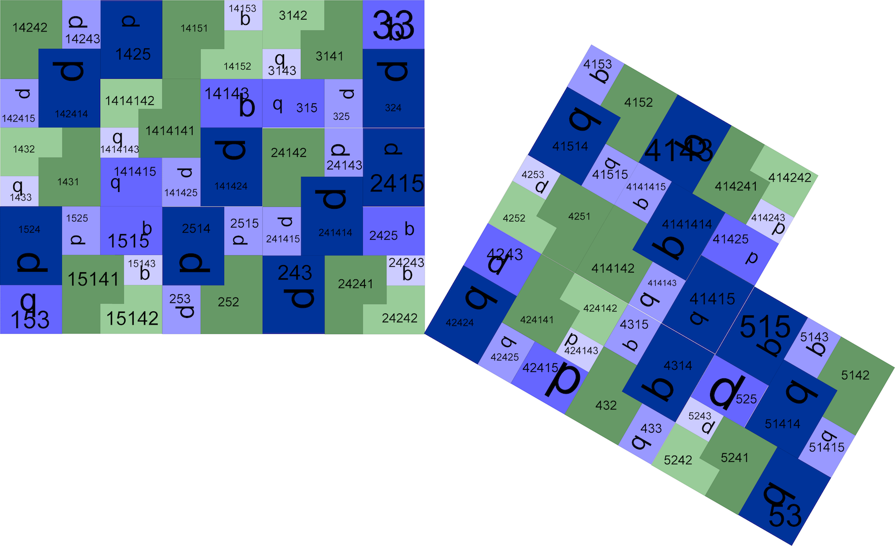
Figure 4. See text.

2.4. Notation for compositions of functions

For $\theta=\theta_{1}\theta_{2}\cdots\theta_{k}\in[N]^{\ast}$, the following notation will be used:

$$f_{\theta} =f_{\theta_{1}}f_{\theta_{2}}\cdots f_{\theta_{k}}$$

$$f_{-\theta} =f_{\theta_{1}}^{-1}f_{\theta_{2}}^{-1}\cdots f_{\theta_{k}}^{-1}=(f_{\theta_{k}\theta_{k-1}\cdots\theta_{1}})^{-1},$$

with the convention that $f_{\theta}$ and $f_{-\theta}$ are the identity function $Id_{\mathbb{R}^{M}}$ if $\theta=\varnothing$. Likewise, for all $\theta\in[N]^{\mathbb{N}}$ and $k\in\mathbb{N}_{0},$ define $\theta|k=\theta_{1}\theta_{2}\cdots\theta_{k}$ and

$$f_{-\theta|k}=f_{\theta_{1}}^{-1}f_{\theta_{2}}^{-1}\cdots f_{\theta_{k}}^{-1}=(f_{\theta_{k}\theta_{k-1}\cdots\theta_{1}})^{-1},$$

with the convention that $f_{-\theta|0}=id$.

For $\theta\in[N]^{\ast}\cup[N]^{\mathbb{N}}$ we define

$$\left|\theta\right|=\left\{\begin{array}[]{cc}k&\text{if }\theta\in[N]^{k},\\ \infty&\text{if }\theta\in[N]^{\mathbb{N}}.\end{array}\right.$$

2.5. Existence and approximation of attractors

Let $\mathbb{H}$ be the nonempty compact subsets of $\mathbb{R}^{M}$. We equip $\mathbb{H}$ with the Hausdorff metric so that it is a complete metric space. Define $\mathbf{F:}\mathbb{H}^{V}\rightarrow\mathbb{H}^{V}$ by

$$\left(\mathbf{F}X\right)_{v}=\left\{x\in f_{e}X_{w}:e\in\mathcal{E}_{v,w},w\in\mathcal{V}\right\}\text{,}$$

for all $X\in\mathbb{H}^{V}$, where $X_{w}$ is the $w^{th}$ component of $X$.

Definition 1.

Define $\theta\in\Sigma_{\infty}$ to be disjunctive if, given any $k\in\mathbb{N}$ and $\omega\in\Sigma_{k}$ there is $p\in\mathbb{N}_{0}$ so that $\omega=\theta_{p+1}\theta_{p+1}...\theta_{p+k}$.

Theorem 1 summarizes some known or readily inferred information regarding the existence, uniqueness, and construction of attractors of $(\mathcal{F},\mathcal{G)}$.

Theorem 1.

Let $\left(\mathcal{F},\mathcal{G}\right)$ be a graph directed IFS.

1. (Contraction on $\mathbb{H}^{V}$) The map $\mathbf{F}:\mathbb{H}^{V}\rightarrow\mathbb{H}^{V}$ is a contraction with contractivity factor $\lambda$. There exists unique $\mathbf{A}=(A^{1},A^{2},...,A^{V})\in\mathbb{H}^{V}$ such that

   $$\mathbf{A=FA}$$

   and

   $$\mathbf{A=}\lim_{k\rightarrow\infty}\mathbf{F}^{k}\mathbf{B}$$

   for all $\mathbf{B}\in\mathbb{H}^{V}$.

2. (Chaos Game on $\mathbb{H}$) There is a unique $A\in\mathbb{H}$ such that

   $$A=\bigcap\limits_{k\in\mathbb{N}}\overline{({\displaystyle\bigcup\limits_{n=k}^{\infty}}x_{n})},$$

   for all $x_{0}\in\mathbb{R}^{m},$ and all disjunctive $\theta=\theta_{1}\theta_{2}...\in\Sigma_{\infty}^{{\dagger}}$. Here

   $$x_{n}=f_{\theta_{n}}(x_{n-1})$$

   for all $n\in\mathbb{N}$ and the bar denotes closure. The set $A$ is related to $\mathbf{A}$ by $A=\cup_{v\in\mathcal{V}}A^{v}.$

3. (Deterministic Algorithm on $\mathbb{H}$) If $B\in\mathbb{H}$ then

   $$A=\lim_{k\rightarrow\infty}\left\{x\in f_{\sigma}(B):\sigma=\sigma_{1}\sigma_{2}...\sigma_{k}\in\Sigma_{k}\right\}.$$

   Also

   $$A^{w}=\lim_{k\rightarrow\infty}\left\{x\in f_{\sigma}(B):\sigma=\sigma_{1}\sigma_{2}...\sigma_{k}\in\Sigma_{k},\sigma_{1}\in\mathcal{E}_{\ast,w}\right\}$$

   for all $w\in\mathcal{V}$.

Proof.

(1) The proof of this is well-known and straightfoward. See for example [6, Chapter 10].

(2) This is a simple generalization of the main result in [8] which applies when $\left|\mathcal{V}\right|=1$.

(3) This follows from (1). ∎

Definition 2.

Using the notation of Theorem 1, $A:=\cup_{v\in\mathcal{V}}A^{v}$ is the attractor of the IFS $\mathcal{(F},\mathcal{G)}$ and $\left\{A^{v}:v\in\mathcal{V}\right\}$ are its components.

We adopt this definition because it is unified with the case $\left|\mathcal{V}\right|=1$, allowing us to work using only of one copy of $\mathbb{R}^{M}$ and to provide a tiling theory that is naturally unified to all cases. See also [3]. Algorithms based on the chaos game that plot and render pictures of attractors in $\mathbb{R}^{M}$ when $\left|\mathcal{V}\right|=1$ can be generalized by restricting the symbolic orbits so that they are consistent with the graph.

In this paper we assume $A^{i}\cap A^{j}=\varnothing$ for $i\neq j$. When this is not the case, components of the attractor can be moved around to ensure that they have empty intersections by means of a simple change of coordinates: the replacements $f_{i}$ $\rightarrow$ $T_{v}f_{i}T_{v}^{-1}$ for all $i\in\mathcal{E}_{v,v}$, $f_{i}$ $\rightarrow$ $T_{v}f_{i}$ for all $i\in\mathcal{E}_{v,\ast}^{{\dagger}}\backslash\mathcal{E}_{v,v}$, $f_{i}$ $\rightarrow$ $f_{i}T_{\upsilon}^{-1}$ for all $i\in\mathcal{E}_{\ast,v}^{{\dagger}}\backslash\mathcal{E}_{v,v}$, where $T_{\upsilon}:\mathbb{R}^{M}\rightarrow\mathbb{R}^{M}$ is for example a translation, moves $A^{v}$ to $T_{\upsilon}A^{v}$ without altering the other components of the attractor.

2.6. The coding map $\pi:\Sigma\rightarrow\mathbb{H(}A)$

For $e\in\mathcal{E}$, let $\overleftarrow{\upsilon}(e),\overrightarrow{\upsilon}(e)\in\mathcal{V}$ be the unique vertices such that $e$ is directed from $\overleftarrow{\upsilon}(e)$ to $\overrightarrow{\upsilon}(e)$.

Definition 3.

Define ${\pi}:\Sigma\rightarrow\mathbb{H(}A)$ by

$$\mathcal{\pi}(\varnothing) =A,$$

$$\mathcal{\pi}(\omega) =f_{\omega}(A^{\overrightarrow{\upsilon}(\omega_{k})})\text{ for all }\omega=\omega_{1}\omega_{2}...\omega_{k}\in\Sigma_{\ast},k\in\mathbb{N}$$

$$\mathcal{\pi}(\sigma) =\lim_{k\rightarrow\infty}\pi(\omega|k)\text{,}\ \text{for all }\sigma\in\Sigma_{\infty},$$

where the limit is with respect to the Hausdorff metric on $\mathbb{H(}A),$ the collection of nonempty compact subsets of $A$.

We call $\Sigma$ the address space or code space and $\pi$ the coding map for the attractor of the graph IFS $\mathcal{(F},\mathcal{G)}$.

Theorem 2.

The map $\pi:\Sigma\rightarrow\mathbb{H(}A)$ is well-defined and continuous. Restricted to $\Sigma_{\infty}$, $\pi$ is a continuous map from $\Sigma_{\infty}$ into $\mathbb{R}^{M}$ and $\pi(\Sigma_{\infty})=\{\pi(\sigma):\sigma\in\Sigma_{\infty}\}=A$.

Proof.

This follows the same lines as for the case $\left|\mathcal{V}\right|=1$ and is well known since the work of Hutchinson [18]. ∎

2.7. Shift maps

Shift maps acting on the symbolic spaces $\Sigma$ and ${\Sigma}^{{\dagger}}$, defined here, will be seen to interact in an important way with coding maps, attractors, and tilings.

The shift $S:[N]^{\ast}\cup[N]^{\infty}\rightarrow[N]^{\ast}\cup[N]^{\infty}$ is defined by $S(\theta_{1}\theta_{2}\cdots\theta_{k})=\theta_{2}\theta_{3}\cdots\theta_{k}$ and $S(\theta_{1}\theta_{2}\cdots)=\theta_{2}\theta_{3}\cdots,$ with the convention that $S\theta_{1}=\varnothing$. A point $\theta\in[N]^{\infty}$ is eventually periodic if there exists $m\in\mathbb{N}_{0}$ and $n\in\mathbb{N}$ such that $S^{m}\theta=S^{m+n}\theta$. In this case we write $\theta=\theta_{1}\theta_{2}\cdots\theta_{m}\overline{\theta_{m+1}\theta_{m+2}\cdots\theta_{m+n}}$.

We have $S(\Sigma)=\Sigma$ and $S({\Sigma}^{{\dagger}})={\Sigma}^{{\dagger}}.$ We write $S:\Sigma\rightarrow\Sigma$ for the restricted map $S|_{\Sigma}$ and likewise write $S:{\Sigma}^{{\dagger}}\rightarrow{\Sigma}^{{\dagger}}$. Note that $S$ is continuous. The metric spaces $\left(\Sigma,d_{\left|\mathcal{F}\right|}\right)$ and $\left({\Sigma}^{{\dagger}},d_{\left|\mathcal{F}\right|}\right)$ are compact shift invariant subspaces of $\left[N\right]^{\ast}\cup\left[N\right]^{\infty}$.

The coding map $\pi:\Sigma\rightarrow\mathbb{H(}A)$ interacts with shift $S:\Sigma\rightarrow\Sigma$ according to

$$f_{\sigma|k}\circ\pi\circ S^{k}\left(\sigma\right)=\pi\left(\sigma\right)$$

for all $\sigma\in\Sigma$, for all $k\in\mathbb{N}$ with $k\leq\left|\sigma\right|$.

3. Tilings

3.1. Tilings in this paper

We use the same definitions of tile, tiling, similitude, scaling ratio, isometry and prototile set as in [12]. For completeness we quote the definitions in this section. A tile is a perfect (i.e. no isolated points) compact nonempty subset of $\mathbb{R}^{M}$. Fix a Hausdorff dimension $0<D_{H}\leq M$. A tiling in $\mathbb{R}^{M}$ is a set of tiles, each of Hausdorff dimension $D_{H}$, such that every distinct pair of tiles is non-overlapping. Two tiles are non-overlapping if their intersection is of Hausdorff dimension strictly less than $D_{H}$. The support of a tiling is the union of its tiles. We say that a tiling tiles its support.

A similitude is an affine transformation $f:{\mathbb{R}}^{M}\rightarrow{\mathbb{R}}^{M}$ of the form $f(x)=\lambda\,O(x)+q$, where $O$ is an orthogonal transformation and $q\in\mathbb{R}^{M}$ is the translational part of $f(x)$. The real number $\lambda>0$, a measure of the expansion or contraction of the similitude, is called its scaling ratio. An isometry is a similitude of unit scaling ratio and we say that two sets are isometric if they are related by an isometry. We write $\mathcal{U}$ to denote the group of isometries on $\mathbb{R}^{M}$ and write $\mathcal{T}$ to denote a specific group contained in $\mathcal{U}$, see above Lemma 2.

The prototile set $\mathcal{P}$ of a tiling $T$ is a set of tiles such that every tile $t\in T$ can be written in the form $\tau(p)$ for some $\tau\in\mathcal{T}$ and $p\in\mathcal{P}$. The tilings constructed in this paper have finite prototile sets.

3.2. A convenient compact tiling space

Let $\mathbb{T}^{{}^{\prime}}$ be the set of all tilings on $\mathbb{R}^{M}$ using a fixed prototile set (and fixed group $\mathcal{T}$). Let $t_{\emptyset}$ be the empty tile of $\mathbb{R}^{M}$. We assume throughout that if $T\in\mathbb{T}^{{}^{\prime}}$ then $t_{\emptyset}\in T$. We may think of $t_{\emptyset}$ as ”the tile at infinity”.

Let $\rho:\mathbb{R}^{M}\rightarrow\mathbb{S}^{M}$ be the usual $M$-dimensional stereographic projection to the $M$-sphere, obtained by positioning $\mathbb{S}^{M}$ tangent to $\mathbb{R}^{M}$ at the origin. Define $\widehat{\rho}:\mathbb{T}^{{}^{\prime}}\rightarrow\mathbb{S}^{M}$ so that $\widehat{\rho}\left(t_{\emptyset}\right)=\mathbb{S}^{M}\backslash\rho(\mathbb{R}^{M})$ is the point on $\mathbb{S}^{M}$ diametric to the origin and

$$\widehat{\rho}\left(T\right)=\left\{\rho\left(t\right):t\in T,t\neq t_{0}\right\}\cup\widehat{\rho}\left(t_{\emptyset}\right)\text{.}$$

Let $\mathbb{H(S}^{M})$ be the non-empty closed (w.r.t. the usual topology on $\mathbb{S}^{M}$) subsets of $\mathbb{S}^{M}.$ Let $d_{\mathbb{H(S}^{M})}$ be the Hausdorff distance with respect to the round metric on $\mathbb{S}^{M}$, so that $(\mathbb{H(S}^{M}),d_{\mathbb{H(S}^{M})})$ is a compact metric space. Let $\mathbb{H(H(S}^{M}))$ be the nonempty compact subsets of $(\mathbb{H(S}^{M}),d_{\mathbb{H(S}^{M})})$, and let $d_{\mathbb{H(H(S}^{M}))}$ be the associated Hausdorff metric. Then $(\mathbb{H(H(S}^{M})),d_{\mathbb{H(H(S}^{M}))})$ is a compact metric space. Finally, define a metric $d_{\mathbb{T}^{\prime}}$ on $\mathbb{T}^{\prime}$ by

$$d_{\mathbb{T}^{\prime}}(T_{1},T_{2})=d_{\mathbb{H(H(S}^{M}))}(\widehat{\rho}\left(T_{1}\right),\widehat{\rho}\left(T_{2}\right))$$

for all $T_{1},T_{2}\in\mathbb{T}^{\prime}$.

Theorem 3.

$\mathbb{(T}^{\prime},d_{\mathbb{T}^{\prime}})$ is a compact metric space.

Proof.

Note that a sequence of tilings in $\mathbb{T}^{\prime}$ may converge to $t_{\emptyset}$, but this cannot happen if all the tilings in a sequence have a nonempty tile in common. ∎

See also [1, 14, 24, 25, 27] where other, mainly equivalent, metrics and topologies on various tiling spaces are defined and discussed.

3.3. Tiling iterated function systems

Definition 4.

Let $\mathcal{F}=\{{\mathbb{R}}^{M};f_{1},f_{2},\cdots,f_{N}\}$, with $N\geq 2$, be an IFS of contractive similitudes where the scaling factor of $f_{n}$ is $\lambda_{n}=s^{a_{n}}$ where $a_{n}\in\mathbb{N}$ and $\gcd\{a_{1},a_{2},\cdots,a_{N}\}=1$ and we define

$$a_{\max}=\max\{a_{i}:i=1,2,\dots,N\}.$$

For $x\in{\mathbb{R}}^{M}$, the function $f_{n}:\mathbb{R}^{M}\rightarrow\mathbb{R}^{M}$ is defined by

$$f_{n}(x)=s^{a_{n}}O_{n}(x)+q_{n}$$

where $O_{n}$ is an orthogonal linear transformation and $q_{n}\in{\mathbb{R}}^{M}$. Let $D_{H}(X)$ be the Hausdorff dimension of $X\subset\mathbb{R}^{M}$. We require that the graph $\mathcal{G}$ be such that

(3.1) $$D_{H}(f_{e}(A^{\overrightarrow{v}(e)})\cap f_{l}(A^{\overrightarrow{v}(l)}))<D_{H}(A)$$

for all $e,l\in\mathcal{E}$ with $e\neq l$. We also require

(3.2) $$A^{i}\cap A^{j}=\varnothing$$

for all $i\neq j$. If these conditions and the requirement on $\mathcal{F}$ above hold, then we say that $\left(\mathcal{F},\mathcal{G}\right)$ is a tiling iterated function system or TIFS.

It might be better to require that $(\mathcal{F}$,$\mathcal{G)}$ obeys the open set condition (OSC) namely, there exists a nonempty bounded open set $U$ so that $f_{i}(U)\subset U$ and $f_{i}(U)\cap f_{j}(U)=\varnothing$ for all $i\neq j$, $i,j\in[N]$.

Note that when $(\mathcal{F}$,$\mathcal{G)}$ obeys the OSC $D_{H}$ can be described elegantly using a spectral radius, see [20], as follows. For given $e,l\in\mathcal{E}$, define

$$\mathcal{V}_{e,l}=\left\{\begin{array}[]{cc}1\text{ }&\text{if }e\text{ follows }l\text{, }\\ 0\text{ }&\text{otherwise.}\end{array}\right.$$

If $(\mathcal{F}$,$\mathcal{G)}$ obeys the OSC then $D_{H}\in(0,M]$ is the unique value such that the spectral radius of the $N\times N$ matrix $\mathcal{V}_{i,j}s^{D_{H}a_{j}}$ equals one. In this case we expect, based on what happens in the case of standard IFS theory, discussed a bit in [12], that Equation 3.1 holds, and our theory applies. In the case $\left|\mathcal{V}\right|=1$ the OSC implies that the Hausdorff dimension of $A$ is strictly greater than the Hausdorff dimension of the set of overlap $\mathcal{O=\cup}_{i\neq j}f_{i}(A)\cap f_{j}(A)$. Similitudes applied to subsets of the set of overlap comprise the sets of points at which tiles may meet. In [4, p.481] we discuss measures of attractors compared to measures of the set of overlap.

3.4. The function $\xi:\Sigma_{\ast}\rightarrow\mathbb{N}_{0}$ and the addresses $\Omega_{k}$

For $\sigma=\sigma_{1}\sigma_{2}\cdots\sigma_{k}\in\Sigma_{\ast}$ define

$$\xi(\sigma)=a_{\sigma_{1}}+a_{\sigma_{2}}+\cdots+a_{\sigma_{k}}\qquad\text{and}\qquad\xi^{-}(\sigma)=a_{\sigma_{1}}+a_{\sigma_{2}}+\cdots+a_{\sigma_{k-1}},$$

and $\xi(\varnothing)=\xi^{-}(\varnothing)=0$. We also write $\sigma^{-}=\sigma_{1}\sigma_{2}\cdots\sigma_{k-1}$ so that

$$\xi^{-}(\sigma)=\xi(\sigma^{-}).$$

Define

$$\Omega_{k} =\{\sigma\in\Sigma_{\ast}:\xi^{-}(\sigma)\leq k<\xi(\sigma)\},$$

$$\Omega_{0} =\left[N\right],$$

for all $k\in\mathbb{N}$ and $\upsilon\in\mathcal{V}$.

3.5. Our tilings $\left\{\Pi\left(\theta\right):\theta\in\Sigma^{{\dagger}}\right\}$

Definition 5.

A mapping $\Pi$ from ${\Sigma}^{{\dagger}}$ to collections of subsets of $\mathbb{H(R}^{M})$ is defined as follows. For $\theta\in\Sigma_{\ast}^{{\dagger}},\theta\neq\left\{\emptyset\right\},$

$$\Pi(\theta_{1}\theta_{2}...\theta_{k}):=\{f_{{}_{-\theta_{1}\theta_{2}...\theta_{k}}}\pi\left(\sigma\right):\sigma\in\Omega_{\xi(\theta_{1}\theta_{2}...\theta_{k})},\sigma_{1}\in\mathcal{E}_{\overrightarrow{\upsilon}(\theta_{k}),\ast}\},$$

and for $\theta\in\Sigma_{\infty}^{{\dagger}}$

$$\Pi(\theta):=\bigcup\limits_{k\in\mathbb{N}}\Pi(\theta|k).$$

Also

$$\mathbb{T}:=\Pi\left(\Sigma^{{\dagger}}\right),\mathbb{T}_{\infty}:=\Pi\left(\Sigma_{\infty}^{{\dagger}}\right),\mathbb{T}_{\ast}:=\Pi\left(\Sigma_{\ast}^{{\dagger}}\right)$$

Definition 6.

We say that $(\mathcal{F},\mathcal{G)}$ is purely self-referential if $\mathcal{E}_{v,v}\neq\varnothing$ for all $v\in\mathcal{V}$.

**If $(\mathcal{F},\mathcal{G)}$ is such that $\mathcal{E}_{v,v}\neq\varnothing$ for at least one $v\in\mathcal{V}$, then by composing functions along paths through vertices for which $\mathcal{E}_{v,v}=\varnothing$, assigning indices to these composed functions, and relabelling the functions and redefining the tiles, we can obtain a self-referential TIFS which presents the essential action of the system.

Theorem 4.

Let $(\mathcal{F},\mathcal{G)}$ be a TIFS.

1. Each set $\Pi(\theta)$ in $\mathbb{T}$ is a tiling of a subset of $\mathbb{R}^{M}$, the subset being bounded when $\theta\in{\Sigma}_{\ast}^{{\dagger}}$ and unbounded when $\theta\in{\Sigma}_{\infty}^{{\dagger}}$.

2. For all $\theta\in{\Sigma}_{\infty}^{{\dagger}}$ the sequence of tilings $\left\{\Pi(\theta|k)\right\}_{k=1}^{\infty}$ is nested according to

   (3.3) $$\Pi(\theta|1)\subset\Pi(\theta|2)\subset\Pi(\theta|3)\subset\cdots\text{ .}$$

3. If $(\mathcal{F},\mathcal{G)}$ is purely self-referential, then for all $\theta\in{\Sigma}^{{\dagger}}$, with $\left|\theta\right|$ sufficiently large, the prototile set for $\Pi(\theta)$ is

   $$\mathcal{P}:=\{s^{i}A^{v}:i\in\left\{1,2,\cdots,a_{\max}\right\},v\in\mathcal{V}\}.$$

4. Let $\mathbb{T}^{\prime}$ to be the set of all tilings with prototile set $\mathcal{P}$. The map

   $$\Pi:{\Sigma}^{{\dagger}}\rightarrow\mathbb{T\subset T}^{\prime}$$

   is continuous from the compact metric space $\left({\Sigma}^{{\dagger}},d_{\left|\mathcal{F}\right|}\right)$ into the compact metric space $(\mathbb{T}^{\prime},d_{\mathbb{T}^{\prime}})$.

5. For all $\theta\in{\Sigma}_{\infty}^{{\dagger}}$

   (3.4) $$\Pi(\theta)=\lim_{k\rightarrow\infty}f_{{}_{-\theta|k}}(\{\pi\left(\sigma\right):\sigma\in\Omega_{\xi(\theta|k)}\}).$$

Proof.

Concerning (5) : Since the components of the attractor are ”just touching” or have empty intersection, we have Equation (3.4). The $k^{th}$ term here is the function $f_{{}_{-\theta|k}}$ applied to the whole attractor (the union of all of the $A^{v}$) ”refined or subdivided” to depth $k$. To say this another way: the set inside the curly parentheses is the whole attractor, the union of its components, partitioned systematically recursively $k$ times. ∎

4. Symbolic structure: canonical symbolic tilings and symbolic inflation and deflation

In this section we develop notation and key results concerning what we might call symbolic tiling theory. In Section 7, we show that these symbolic structures and relationships are conjugate to counterparts in self-similar tiling theory. These concepts are also interesting because of their combinatorial structure.

Define

$$\Sigma_{\ast}^{v}=\{\sigma\in\Sigma_{\ast}:\sigma_{1}\in\mathcal{E}_{\ast,v}\},\Sigma_{\infty}^{v}=\{\sigma\in\Sigma_{\infty}:\sigma_{1}\in\mathcal{E}_{\ast,v}\},\Sigma^{v}=\{\sigma\in\Sigma:\sigma_{1}\in\mathcal{E}_{\ast,v}\}$$

for all $v\in\mathcal{V}$, and analogously define $\Sigma_{\ast}^{{\dagger}v},\Sigma_{\infty}^{{\dagger}v},\Sigma^{{\dagger}v}.$ Define what we might call canonical symbolic tilings

$$\Omega_{k}^{v}=\{\sigma\in\Sigma_{\ast}^{v}:\xi^{-}(\sigma)\leq k<\xi(\sigma)\},$$

for all $k\in\mathbb{N}$ and $\upsilon\in\mathcal{V}$. Note that

$$\Omega_{k}=\cup_{v\in\mathcal{V}}\Omega_{k}^{v}\text{ and }\Omega_{0}^{v}=\{j\in[N]:\sigma_{1}\in\mathcal{E}_{\ast,v}\}$$

We write $\Omega_{k}^{(v)}$ to mean any one of the sets $\Omega_{k}$ and $\Omega_{k}^{v}$ for $v\in\mathcal{V}$. The following lemma tells us that $\Omega_{k+1}^{(v)}$ can be obtained from $\Omega_{k}^{(v)}$ by adding symbols to the right-hand end of some strings in $\Omega_{k}^{(v)}$ and leaving the other strings unaltered.

Lemma 1.

(Symbolic Splitting) For all $k\in\mathbb{N}$ and $v\in\mathcal{V}$ the following relations hold:

$$\Omega_{k+1}^{(v)}=\left\{\sigma\in\Omega_{k}^{(v)}:k+1\leq\xi\left(\sigma\right)\right\}\cup\left\{\sigma j\in\Sigma_{\ast}^{\left(v\right)}:\sigma\in\Omega_{k}^{(v)},k=\xi\left(\sigma\right)\right\}\text{.}$$

Proof.

Follows at once from definition of $\Omega_{k}^{(v)}$. ∎

This defines symbolic inflation or ”splitting and expansion” of $\Omega_{k}^{(v)}$, some words in $\Omega_{k+1}^{(v)}$ being the same as in $\Omega_{k}^{(v)}$ while all the others are ”split”. The inverse operation is symbolic deflation or ”amalgamation and shrinking”, described by a function

$$\alpha_{s}:\Omega_{k+1}^{(v)}\rightarrow\Omega_{k}^{(v)}\text{, }\alpha_{s}(\Omega_{k+1}^{(v)})=\Omega_{k}^{(v)}$$

The operation $\alpha_{s}^{-1}$, whereby $\Omega_{k+1}^{(v)}$ is obtained from $\Omega_{k}^{(v)}$ by adding symbols to the right-hand end of some words in $\Omega_{k}^{(v)}$ and leaving other words unaltered, is symbolic splitting and expansion. In particular, we can define a map $\alpha_{s}:\Omega_{k+1}^{(v)}\rightarrow\Omega_{k}^{(v)}$ for all $k\mathbb{\in N}_{0}$ according to $\alpha_{s}(\theta)$ is the unique $\omega\in\Omega_{k}^{(v)}$ such that $\theta=\omega\beta$ for some $\beta\in\Sigma_{\ast}$. Note that $\beta$ may be the empty string. That is, symbolic amalgamation and shrinking $\alpha_{s}$ is well-defined on $\Sigma_{\ast}$.

This tells us that we can use $\Omega_{k}^{(v)}$ to define a partition of $\Omega_{m}^{(v)}$ for $m\geq k$. The partition of $\Omega_{k+j}^{(v)}$ is $\Omega_{k+j}^{(v)}/\sim$ where $x\sim y$ if $\alpha_{s}^{j}(x)=\alpha_{s}^{j}(y)$. To say this another way:

Corollary 1.

(Symbolic Partitions) For all $m\geq k\geq 0,$ the set $\Omega_{k}^{(v)}$ defines a partition $P_{m,k}^{(v)}$ of $\Omega_{m}^{(v)}$ according to $p\in P_{m,k}^{(v)}$ if and only if there is $\omega\in\Sigma_{\ast}$ such that

$$p=\{\omega\beta\in\Omega_{m}^{(v)}:\beta\in\Omega_{k}^{(v)}\}.$$

Proof.

This follows from Lemma 1: for any $\theta\in\Omega_{m}^{(v)}$ there is a unique $\omega\in\Omega_{k}^{(v)}$ such that $\theta=\omega\beta$ for some $\beta\in\Sigma_{\ast}$. Each word in $\Omega_{m}^{(v)}$ is associated with a unique word in $\Omega_{k}^{(v)}$. Each word in $\Omega_{k}^{(v)}$ is associated with a set of words in $\Omega_{m}^{(v)}$. ∎

According to Lemma 1, $\Omega_{k+1}^{(v)}$ may be calculated by tacking words (some of which may be empty) onto the right-hand end of the words in $\Omega_{k}^{(v)}$. Now we reverse the description, expressing $\Omega_{k}^{(v)}$ as a union of predecessors ($\Omega_{j}^{(v)}$s with $j<k$) of $\Omega_{k}^{(v)}$ with words tacked onto their left-hand ends. The following structural result will reappear (**make explicit) in what follows.

Corollary 2.

(Symbolic Predecessors) For all $k\geq a_{\max}+l$, for all $v\in\mathcal{V}$, for all $l\in\mathbb{N}_{0},$

$$\Omega_{k}^{\left(v\right)}=\bigsqcup\limits_{\omega\in\Omega_{l}^{\left(v\right)}}\omega\Omega_{k-\xi\left(\omega\right)}^{\left(\overrightarrow{v}\left(\omega\right)\right)}$$

Proof.

It is easy to check that the r.h.s. is contained in the l.h.s.

Conversely, if $\theta\in\Omega_{k}^{\left(v\right)}$ then there is unique $\omega\in\Omega_{l}^{\left(v\right)}$ such that $\theta=\omega\beta$ for some $\beta\in\Sigma_{\ast}$ by Corollary 1. Because $\omega\beta\in\Sigma_{\ast}$ it follows that $\beta_{1}$ is an edge that that starts where the last edge in $\omega$ is directed to, namely the vertex $\overrightarrow{v}\left(\omega\right)$. Finally, since $\xi\left(\omega\beta\right)=\xi\left(\omega)+\xi(\beta\right)$ it follows that $\beta\in\Omega_{k-\xi\left(\omega\right)}^{\overrightarrow{v}\left(\omega\right)}$. ∎

5. Canonical tilings and their relationship to $\Pi(\theta)$

Definition 7.

We define sequences of tilings by

$$T_{k}=s^{-k}\pi(\Omega_{k}),\text{ }T_{k}^{v}:=s^{-k}\pi(\Omega_{k}^{v})$$

$k\in\mathbb{N},v\in\mathcal{V}$, to be called the canonical tilings of the TIFS $(\mathcal{F},\mathcal{G)}.$

A canonical tiling may be written as a disjoint union of copies of other canonical tilings. By a copy of a tiling $T$ we mean $ET$ for some $E\in\mathcal{T}$, where $\mathcal{T}$ is the set of all isometries of $\mathbb{R}^{M}$ generated by the functions of $\mathcal{F}$ together with multiplication by $s.$

Lemma 2.

For all $k\geq a_{\max}+l$, for all $l\in\mathbb{N}_{0},$ for all $v\in[N]$

$$T_{k}^{v}=\bigsqcup\limits_{\omega\in\Omega_{l}^{v}}E_{k,\omega}T_{k-\xi\left(\omega\right)}^{\overrightarrow{v}\left(\omega\right)}\text{ and }T_{k}=\bigsqcup\limits_{\omega\in\Omega_{l}}E_{k,\omega}T_{k-\xi\left(\omega\right)}^{\overrightarrow{v}\left(\omega\right)}$$

where $E_{k,\omega}=s^{-k}f_{\omega}s^{k-e(\omega)}\in\mathcal{T}$ is an isometry.

Proof.

Direct calculation. ∎

Theorem 5.

For all $\theta\in\Sigma_{\ast}^{{\dagger}},$

$$\Pi(\theta)=E_{\theta}T_{\xi(\theta)}^{\overrightarrow{v}(\theta_{\left|\theta\right|})},$$

where $E_{\theta}=f_{-\theta}s^{\xi(\theta)}$. Also if $l\in\mathbb{N}_{0},$ and $\xi(\theta)\geq a_{\max}+l$, then

$$\Pi(\theta)=\bigsqcup\limits_{\omega\in\Omega_{l}^{\overrightarrow{v}(\theta_{\left|\theta\right|})}}E_{\theta,\omega}T_{\xi(\theta)-\xi\left(\omega\right)}^{\overleftarrow{v}\left(\omega\right)}$$

where $E_{\theta,\omega}=f_{{}_{-\theta}}f_{\omega}s^{\xi(\theta)-e(\omega)}$ is an isometry.

Proof.

Writing $\theta=\theta_{1}\theta_{2}...\theta_{k}$ so that $\left|\theta\right|=k,$ we have from the definitions

$$\Pi(\theta_{1}\theta_{2}...\theta_{k}) =f_{{}_{-\theta_{1}\theta_{2}...\theta_{k}}}\{\pi\left(\sigma\right):\sigma\in\Omega_{\xi(\theta_{1}\theta_{2}...\theta_{k})}^{\overrightarrow{\upsilon}(\theta_{k})}\}$$

$$=f_{{}_{-\theta_{1}\theta_{2}...\theta_{k}}}s^{\xi(\theta_{1}\theta_{2}...\theta_{k})}s^{-\xi(\theta_{1}\theta_{2}...\theta_{k})}\{\pi(\sigma):\sigma\in\Omega_{\xi(\theta_{1}\theta_{2}...\theta_{k})}^{\overrightarrow{\upsilon}(\theta_{k})}\}$$

$$=E_{\theta_{1}\theta_{2}...\theta_{k}}T_{\xi(\theta_{1}\theta_{2}...\theta_{k})}^{\overrightarrow{\upsilon}(\theta_{k})}$$

which demonstrates that $\Pi(\theta)=E_{\theta}T_{\xi(\theta)}^{\overrightarrow{\upsilon}(\theta_{\left|\theta\right|})}$where $E_{\theta}=f_{-\theta}s^{\xi(\theta)}$.

The last statement of the theorem follows similarly from Lemma 2. ∎

6. All tilings in $\mathbb{T}^{\infty}$ are quasiperiodic

We recall from [12] the following definitions. A subset $P$ of a tiling $T$ is called a patch of $T$ if it is contained in a ball of finite radius. A tiling $T$ is quasiperiodic (also called repetitive) if, for any patch $P$, there is a number $R>0$ such that any disk centered at a point in the support of $T$ and is of radius $R$ contains an isometric copy of $P$. Two tilings are locally isomorphic if any patch in either tiling also appears in the other tiling. A tiling $T$ is self-similar if there is a similitude $\psi$ such that $\psi(t)$ is a union of tiles in $T$ for all $t\in T$. Such a map $\psi$ is called a self-similarity.

Theorem 6.

Let $(\mathcal{F},\mathcal{G)}$ be a tiling IFS.

1. Each tiling in $\mathbb{T}_{\infty}$ is quasiperiodic and each pair of tilings in $\mathbb{T}_{\infty}$ are locally isomorphic.

2. If $\theta\in{\Sigma}_{\infty}^{{\dagger}}$ is eventually periodic, then $\Pi(\theta)$ is self-similar. In fact, if $\theta=\alpha\overline{\beta}$ for some $\alpha,\beta\in{\Sigma}_{\infty}^{{\dagger}}$ then $f_{-\alpha}f_{-\beta}\left(f_{-\alpha}\right)^{-1}\Pi(\theta)$ is a self-similarity.

Proof.

This uses Theorem 5, and follows similar lines to [12, proof of Theorem 2]. ∎

7. Addresses

Addresses, both relative and absolute, are described in [12] for the case $\left|\mathcal{V}\right|=1$. See also [3]. Here we add information, and generalize. The relationship between these two types of addresses is subtle and central to our proof of Theorem 9.

7.1. Relative addresses

Definition 8.

The relative address of $t\in T_{k}^{(v)}$ is defined to be $\varnothing.\pi^{-1}s^{k}(t)\in\varnothing.\Omega_{k}^{(v)}$. The relative address of a tile $t\in T_{k}$ depends on its context, its location relative to $T_{k}$, and depends in particular on $k\in\mathbb{N}_{0}$. Relative addresses also apply to the tiles of $\Pi(\theta)$ for each $\theta\in\Sigma_{\ast}^{{\dagger}}$ because $\Pi(\theta)=E_{\theta}T_{\xi(\theta)}^{\overleftarrow{\upsilon}(\theta_{\left|\theta\right|})}$ where $E_{\theta}=f_{-\theta}s^{\xi(\theta)}$ (by Theorem 5) is a known isometry applied to $T_{\xi(\theta)}$. Thus, the relative address of $t\in\Pi(\theta)$ (relative to $\Pi(\theta)$) is $\varnothing.\pi^{-1}f_{-\theta}^{-1}(t)$, for $\theta\in\Sigma_{\ast}^{{\dagger}}$.

Lemma 3.

The tiles of $T_{k}$ are in bijective correspondence with the set of relative addresses $\varnothing.\Omega_{k}$. Also the tiles of $T_{k}^{v}$ are in bijective correspondence with the set of relative addresses $\varnothing.\Omega_{k}^{v}$.

Proof.

We have $T_{k}=s^{-k}\pi(\Omega_{k})$ so $s^{-k}\pi$ maps $\Omega_{k}$ onto $T_{k}$. Also the map $s^{-k}\pi:\Omega_{k}\rightarrow T_{k}$ is one-to-one: if $\beta\neq\gamma,$ for $\beta,\gamma\in\Sigma_{\ast}$ then $f_{\beta}(A)\neq f_{\gamma}(A)$ because $t=$ $s^{-k}\pi(\beta)=s^{-k}\pi(\gamma)$with $\beta,\gamma\in T_{k}$ implies $\beta=\gamma$. ∎

For precision we should write ”the relative address of $t$ relative to $T_{k}$” or equivalent: however, when the context $t\in T_{k}$ is clear, we may simply refer to ”the relative address of $t$”.

Example 1.

(Standard 1D binary tiling) For the IFS $\mathcal{F}_{0}=\{\mathbb{R};f_{1},f_{2}\}$ with $f_{1}(x)=0.5x,f_{2}(x)=$ $0.5x+0.5$ we have $\Pi(\theta)$ for $\theta\in\Sigma_{\ast}^{{\dagger}}$ is a tiling by copies of the tile $t=[0,0.5]$ whose union is an interval of length $2^{\left|\theta\right|}$ and is isometric to $T_{\left|\theta\right|}$ and represented by $tttt....t$ with relative addresses in order from left to right

$$\varnothing.111...11,\varnothing.111...12,\varnothing.111...21,....,\varnothing.222...22,$$

the length of each string (address) being $\left|\theta\right|+1.$ Notice that here $T_{k}$ contains $2^{\left|\theta\right|}-1$ copies of $T_{0}$ (namely tt) where a copy is $ET_{0}$ where $E\in\mathcal{T}_{\mathcal{F}_{0}}$, the group of isometries generated by the functions of $\mathcal{F}_{0}$.

Example 2.

(Fibonacci 1D tilings) $\mathcal{F}_{1}\mathcal{=\{}ax,a^{2}x+1-a^{2},a+a^{2}=1,$ $a>0\},$ $\mathcal{T=T}_{\mathcal{F}_{1}}$ is the largest group of isometries generated by $\mathcal{F}_{1}$. The tiles of $\Pi(\theta)$ for $\theta\in\Sigma_{\ast}^{{\dagger}}$ are isometries that belong to $\mathcal{T}_{\mathcal{F}_{1}}$ applied to the tiling of [0,1] provided by the IFS, writing the tiling $\Pi(\varnothing)=T_{0}$ as $ls$ where $l$ is a copy of $[0,a]$ and (here) $s$ is a copy of $[0,a^{2}]$ we have:

$T_{0}=ls$ has relative addresses $\varnothing.1,\varnothing.2$ (i.e. the address of $l$ is $1$ and of $s$ is $2$)

$T_{1}=lsl$ has relative addresses $\varnothing.11,\varnothing.12,\varnothing.2$

$T_{2}=lslls$ has relative addresses $\varnothing.111,\varnothing.112,\varnothing.12,\varnothing.21,\varnothing.22$

$T_{3}=lsllslsl$ has relative addresses $\varnothing.1111,\varnothing.1112,\varnothing.112,\varnothing.121,\varnothing.122,\varnothing.211,\varnothing.212,22$

We remark that $T_{k}$ comprises $F_{k+1}$ distinct tiles and contains exactly $F_{k}$ copies (under maps of $\mathcal{T}_{\mathcal{F}_{1}}$) of $T_{0}$, where $\{F_{k}:k\in\mathbb{N}_{0}\}$ is a sequence of Fibonacci numbers $\{1,2,3,5,8,13,21,...\}$.

Note that $T_{4}=lsllslsllslls$ contains two ”overlapping” copies of $lslls$.

7.2. Absolute addresses

The set of absolute addresses associated with $(\mathcal{F},\mathcal{G)}$ is

$$\mathbb{A}:=\{\theta.\omega:\theta\in\Sigma_{\ast}^{{\dagger}},\,\omega\in\Omega_{\xi(\theta)}^{\overleftarrow{\upsilon}(\theta_{\left|\theta\right|})},\,\theta_{\left|\theta\right|}\neq\omega_{1}\}.$$

Define $\widehat{\pi}:\mathbb{A\rightarrow\{}t\in T:T\in\mathbb{T\}}$ by

$$\widehat{\pi}(\theta.\omega)=f_{-\theta}.f_{\omega}(A).$$

The condition $\theta_{\left|\theta\right|}\neq\omega_{1}$ is imposed. We say that $\theta.\omega$ is an absolute address of the tile $f_{-\theta}.f_{\omega}(A)$. It follows from Definition 4 that the map $\widehat{\pi}$ is surjective: every tile of $\mathbb{\{}t\in T:T\in\mathbb{T\}}$ possesses at least one absolute address.

In general a tile may have many different absolute addresses. The tile $[1,1.5]$ of Example 1 has the two absolute addresses $1.21$ and $21.211$.

7.3. Relationship between relative and absolute addresses

Theorem 7.

If $t\in\Pi(\theta)\backslash\Pi(\varnothing)$ with $\theta\in\Sigma_{\ast}^{{\dagger}}$ has relative address $\omega$ relative to $\Pi(\theta),$ then an absolute address of $t$ is $\theta_{1}\theta_{2}...\theta_{l}.S^{\left|\theta\right|-l}\omega$ where $l\in\mathbb{N}$ is the unique index such that

(7.1) $$t\in\Pi(\theta_{1}\theta_{2}...\theta_{l})\text{ and }t\notin\Pi(\theta_{1}\theta_{2}...\theta_{l-1})$$

(If $t\in\Pi(\varnothing)$, then the unique absolute address of $t$ is $\emptyset.n$ for some $n\in N$.)

Proof.

Recalling that

$$\Pi(\varnothing)\subset\Pi(\theta_{1})\subset\Pi(\theta_{1}\theta_{2})\subset...\subset\Pi(\theta_{1}\theta_{2}...\theta_{\left|\theta\right|-1})\subset\Pi(\theta),$$

we have disjoint union

$$\Pi(\theta)=\Pi(\varnothing)\cup\left(\Pi(\theta_{1})\backslash\Pi(\varnothing)\right)\cup\left(\Pi(\theta_{1}\theta_{2})\backslash\Pi(\theta_{1})\right)\cup...\cup\left(\Pi(\theta)\backslash\Pi(\theta_{1}\theta_{2}...\theta_{\left|\theta\right|-1})\right).$$

So there is a unique $l$ such that Equation (7.1) is true. Since $t\in\Pi(\theta)$ has relative address $\omega$ relative to $\Pi(\theta)$ we have

$$\omega=\varnothing.\pi^{-1}f_{-\theta}^{-1}(t)$$

and so an absolute adddress of $t$ is

$$\theta.\omega|_{cancel}=\theta.\pi^{-1}f_{-\theta}^{-1}(t)|_{cancel}$$

where $|_{cancel}$ means equal symbols on either side of $"."$ are removed until there is a different symbol on either side. Since $t\in\Pi(\theta_{1}\theta_{2}...\theta_{l})$ the terms $\theta_{l+1}\theta_{l+2}...\theta_{\left|\theta\right|}$ must cancel yielding the absolute address

$$\theta.\omega|_{cancel}=\theta_{1}\theta_{2}...\theta_{l}.\omega_{|\theta|-l+1}...\omega_{|\omega|}$$

∎

8. Local rigidity and its consequences

8.1. Definition of locally rigid

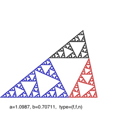
Figure 5. Attractor of a rigid TIFS.

Let $\mathcal{T}$ be the group of isometries generated by the set of maps of $\mathcal{F}$, and let $\mathcal{U}$ be the group of all isometries on $\mathbb{R}^{M}$. Let $\mathcal{T}^{\prime}\subset\mathcal{T}$ be the groupoid of isometries of the form $f_{-\theta}f_{\sigma}$ where $\sigma\in\Sigma_{\ast},\theta\in\Sigma_{\ast}^{{\dagger}}$ and $\overleftarrow{v}(\sigma_{1})\in\overleftarrow{v}(\theta_{\left|\theta\right|}).$

Definition 9.

The family of tilings $\mathbb{T}:=\left\{\Pi(\theta):\theta\in\Sigma^{{\dagger}}\right\},$ and the TIFS $(\mathcal{F},\mathcal{G)}$, are said to be locally rigid when the following two statements are true: (i) if $E\in\mathcal{T}$ is such that $T_{0}^{v}\cap E_{2}T_{0}^{w}$ tiles $A^{v}\cap EA^{w}$ then $E=id$ and $v=w$; (ii) there is only one symmetry of each $A^{v}$ contained in $\mathcal{T}^{\prime}$.

The TIFS $(\mathcal{F},\mathcal{G)}$ is said to be rigid if statements (i) and (ii) are true when $\mathcal{T}^{\prime}$ is replaced by $\mathcal{U}$.

Figure 5 illustrates the attractor of a locally rigid system. The TIFS in Example 2 is not rigid but it is locally rigid. The notion of a rigid tiling was introduced for the case $\left|\mathcal{V}\right|=1$ in [12].

8.2. Main Theorem

We define $\mathbb{Q}:=\{ET:E\in\mathcal{T}$, $T\in\mathbb{T\}}$ and $\mathbb{Q}^{\prime}:=\{ET:E\in\mathcal{T}$, $T\in\mathbb{T},\mathbb{\ }T\neq T_{0}^{v},v\in\mathcal{V}\mathbb{\}}$.

Definition 10.

Let $\mathcal{F}$ be a locally rigid IFS. Any tile in $\mathbb{Q}$ that is isometric to $s^{a_{\max}}A^{v}$ is called a small tile, and any tile that is isometric to $sA^{v}$ is called a large tile. We say that a tiling $P\in\mathbb{Q}$ comprises a set of partners if $P=ET_{0}^{v}$ for some $E\in\mathcal{T}$, $v\in\mathcal{V}$. Given $Q\in\mathbb{Q}$ we define $partners(Q)$ to be the set of all sets of partners in $Q$.

The terminology of large and small tiles is useful in discussing some examples. If a tiling $T\in\mathbb{Q}$ is locally rigid, then each set of partners in $T$ has no partners in common with any other set of partners in $T$.

Define for convenience:

$$\Lambda_{k}^{v} =\{\sigma\in\Sigma_{\ast}:\xi(\sigma)=k,\overleftarrow{v}(\sigma_{1})=v\}\subset\Omega_{k-1}^{v}$$

$$\Lambda_{k} =\cup_{v}\Lambda_{k}^{v}\subset\Omega_{k-1}$$

Theorem 8.

Let $\mathcal{F}$ be locally rigid and let $T_{k}$ be given.

(i) There is a bijective correspondence between $\Lambda_{k}^{v}$ and the set of copies $ET_{0}^{v}\subset T_{k}$ with $E\in\mathcal{T}$.

(ii) If $ET_{0}^{v}\subset T_{k}$ for some $E\in\mathcal{T}$, then there is unique $\sigma\in\Lambda_{k}^{v}$ such that

$$E=E_{\sigma_{\left|\sigma\right|}\sigma_{\left|\sigma\right|-1}...\sigma_{1}}^{-1}=(f_{-\sigma_{\left|\sigma\right|}\sigma_{\left|\sigma\right|-1}...\sigma_{1}}s^{k})^{-1}=s^{-k}f_{\sigma}$$

Proof.

(i) If $(\mathcal{F},\mathcal{G})$ is locally rigid, then given the tiling $ET_{k}$ with $E\in\mathcal{T}$ we can identify $E$ uniquely. The relative addresses of tiles in $ET_{k}$ may then be calculated in tandem by repeated application of $\alpha^{-1}$. Each tile in $ET_{0}$ is associated with a unique relative addresses in $\Omega_{0}=[N]$. Now assume that, for all $l=0,1,...,k,$ we have identified the tiles of $ET_{l}$ with their relative addresses (relative to $T_{l}$). These lie in $\Omega_{l}$. Then the relative addresses of the tiles of $ET_{k+1}$ (relative to $T_{k+1})$ may be calculated from those of $ET_{k}$ by constructing the set of sets $s^{-1}ET_{k}$, and then splitting the images of large tiles, namely those that are of the form $s^{-1}FA^{v}$ for some $v\in\mathcal{V}$ and $F\in\mathcal{T}$ , to form nonintersecting sets of partners of the form $\{Ff_{i}(A^{\overleftarrow{v}(i)}):i\in\mathcal{E}_{v,\ast}\}$, assigning to these ”children of the split” the relative addresses of their parents (relative to $T_{k}$) together with an additional symbol $i\in\left[N\right]$ added on the right-hand end according to its relative address relative to the copy of $T_{0}$ to which it belongs. By local rigidity, this can be done uniquely. The relative addresses (relative to $T_{k+1}$) of the tiles in $s^{-1}ET_{k}$ that are not split and so are simply $s^{-1}$ times as large as their predecessors, are the same as the relative addresses of their predecessors relative to $T_{k}.$

(ii) It follows in particular that if $\mathcal{F}$ is locally rigid and $E^{\prime}T_{0}\subset T_{k}$, then the relative addresses of the tiles of $E^{\prime}T_{0}$ must be $\{\varnothing.\sigma_{1}...\sigma_{\left|\sigma\right|}i:i\in[N]\}$ for some $\sigma_{1}...\sigma_{\left|\sigma\right|}\in\Sigma_{\ast}$ with $\xi(\sigma_{1}...\sigma_{\left|\sigma\right|})=k$. In this case we say that the relative address of $E^{\prime}T_{0}$ (relative to $T_{k}$) is $\varnothing.\sigma_{1}...\sigma_{\left|\sigma\right|}$. ∎

Theorem 9.

Let $(\mathcal{F},\mathcal{G)}$ be locally rigid. Then $\Pi(\theta)=E\Pi(\psi)$ for some $E\in\mathcal{T}$, $\theta,\psi\in\Sigma^{{\dagger}}$if and only if there are $p,q\in\mathbb{N}_{0}$ such that $\xi(\theta|p)=\xi(\psi|q),$ $E=E_{\theta|p}E_{\psi|q}^{-1}$ and $S^{p}\theta=S^{q}\psi$.

Proof.

If there are $p,q\in\mathbb{N}_{0}$ such that $\xi(\theta|p)=\xi(\psi|q),$ $E=E_{\theta|p}E_{\psi|q}^{-1}$ and $S^{p}\theta=S^{q}\psi\theta\psi$

$$\Pi(\theta) =\bigsqcup\limits_{m\in\mathbb{N}_{0}}f_{-\theta|\left(p+m\right)}s^{\xi\left(\theta|\left(p+m\right)\right)}T_{\xi\left(\theta|\left(p+m\right)\right)}$$

$$=f_{-\theta|p}\bigsqcup\limits_{m\in\mathbb{N}_{0}}f_{-\psi_{q+1}\psi_{q+2}...\psi_{q+m}}s^{\xi\left(\psi_{q+1}\psi_{q+2}...\psi_{q+m}\right)}s^{\xi(\psi|q)}T_{\xi(\psi|q+m)}$$

$$=f_{-\theta|p}f_{-\psi|q}^{-1}\bigsqcup\limits_{m\in\mathbb{N}_{0}}f_{-\psi|\left(q+m\right)}s^{\xi\left(\psi|\left(q+m\right)\right)}T_{\xi\left(\psi|\left(q+m\right)\right)}$$

$$=E_{\theta|p}E_{\psi|q}^{-1}\Pi(\psi)$$

This completes the proof in one direction.

To prove the converse we suppose that $\mathcal{F}$ is locally rigid and that $\Pi(\theta)=E\Pi(\psi)$ for some $E\in\mathcal{T}$, where $\theta,\psi\in\Sigma^{{\dagger}}$. Let $m$ be any integer such that $E\Pi(\varnothing)\subset\Pi(\theta|m).$ It follows that

$$E_{\theta|m}^{-1}E\Pi(\varnothing)\subset T_{\xi(\theta|m)}$$

Then by Theorem 8 (ii) the set of relative addresses (relative to $T_{\xi(\theta|m)}$) of copies of $T_{0}$ in $\Pi(\theta|m)$ is

$$\left\{\sigma i:i\in[N],\sigma\in\Sigma_{\ast},\xi(\sigma)=\xi(\theta|m)\right\}.$$

It follows that $E_{\theta|m}^{-1}E\Pi(\varnothing)=E_{\sigma_{|\sigma|}\sigma_{|\sigma|-1}...\sigma_{1}}^{-1}\Pi(\varnothing)$ for some unique $\sigma=\sigma_{1}\sigma_{2}...\sigma_{|\sigma|-1}\sigma_{|\sigma|}$ such that $\xi(\sigma)=\xi(\theta|m).$ It follows that

$$E=E_{\theta|m}E_{\sigma_{|\sigma|}\sigma_{|\sigma|-1}...\sigma_{1}}^{-1},$$

where we have used local rigidity. We know the absolute addresses of the tiles of $\Pi(\varnothing)\subset\Pi(\theta|m)$ are

$$\left\{\theta_{1}\theta_{2}...\theta_{m}.\theta_{m}...\theta_{2}\theta_{1}i|_{cancel}\text{ for }i\in[N]\right\}.$$

Given $E=E_{\theta|m}E_{\sigma_{|\sigma|}\sigma_{|\sigma|-1}...\sigma_{1}}^{-1},$ the absolute addresses of $E\Pi(\varnothing)\subset\Pi(\theta|m)$ are then $\left\{\theta_{1}\theta_{2}...\theta_{m}.\sigma i|_{cancel}\text{ for }i\in[N]\right\}.$ Since $\Pi(\theta)=E\Pi(\psi),$

$$\psi_{1}\psi_{2}...\psi_{\left|\sigma\right|}=\sigma_{\left|\sigma\right|}\sigma_{\left|\sigma\right|-1}...\sigma_{1}$$

and thus

$$E=E_{\theta|m}E_{\psi_{1}\psi_{2}...\psi_{\left|\sigma\right|}}^{-1}$$

where $\xi\left(\psi_{1}\psi_{2}...\psi_{\left|\sigma\right|}\right)=\xi\left(\sigma\right)=\xi(\theta|m)$.

Now let $k\in\mathbb{N}$ and consider the two sets $\Pi(\varnothing)$ and $E\Pi(\varnothing)$ both of which belong to $\Pi(\theta|m)=E_{\theta|m}T_{\xi(\theta|m)}$ which in turn is contained in $\Pi(\theta|m+k)=E_{\theta|\left(m+k\right)}T_{\xi(\theta|\left(m+k\right))}$. We are going to calculate the relative addresses of both $\Pi(\varnothing)$ and $E\Pi(\varnothing)$ relative to $T_{\xi(\theta|\left(m+k\right))}$ in terms of their relative addresses relative to $T_{\xi(\theta|m)}$. Using Definition 8 we find: the relative address of $t\in\Pi(\theta|m)\subset\Pi(\theta|m+k)$ relative to $T_{\xi(\theta|m)}$ is $\omega=\pi^{-1}(s^{\xi(\theta|m)}E_{\theta|m}^{-1}t)$ and relative to $T_{\xi(\theta|\left(m+k\right))}$ it is $\widetilde{\omega}=\pi^{-1}(s^{\xi(\theta|\left(m+k\right))}E_{\theta|\left(m+k\right)}^{-1}t)$. It follows that $\widetilde{\omega}=\theta_{m+k}\theta_{m+k-1}...\theta_{m+1}\omega.$ Hence the relative addresses of $\Pi(\varnothing)$ and $E\Pi(\varnothing)$ relative to $T_{\xi(\theta|\left(m+k\right))}$ are $\varnothing.\theta_{m+k}\theta_{m+k-1}...\theta_{m+1}\theta_{m}...\theta_{1}$ and $\varnothing.\theta_{m+k}\theta_{m+k-1}...\theta_{m+1}\psi_{\left|\sigma\right|}\psi_{\left|\sigma\right|-1}...\psi_{1}$. It follows that $S^{\left|\sigma\right|}\psi=S^{m}\theta$. ∎

Corollary 3.

If $\mathcal{(F},\mathcal{V)}$ is locally rigid, then $\Pi(\theta)=E\Pi(\theta)$ if and only if $E=id$.

Corollary 4.

If $\mathcal{(F},\mathcal{V)}$ is locally rigid, then $\Pi:\Sigma^{{\dagger}}\rightarrow\mathbb{T}$ is a homeomorphism.

9. Inflation and deflation

If $(\mathcal{F},\mathcal{G)}$ is locally rigid, then the operations of inflation or ”expansion and splitting” of tilings in $\mathbb{Q}$, and deflation or ”amalgamation and shrinking” of tilings in $\mathbb{Q}^{\prime}$ are well-defined. We handle these concepts with the operators $\alpha^{-1}$ and its inverse $\alpha,$ respectively, also used in [12].

Theorem 10.

Let $\mathcal{F}$ be a locally rigid IFS. The amalgamation and shrinking (deflation) operation $\alpha:\mathbb{Q}^{\prime}\mathbb{\rightarrow Q}$ is well-defined by

$$\alpha Q^{\prime}=\{st:t\in Q\backslash partners(Q^{\prime})\}\cup\bigsqcup\{sEA^{v}:E\in\mathcal{T},ET_{0}^{v}\subset partners(Q^{\prime}),v\in\mathcal{V}\}$$

for all $Q^{\prime}\in\mathbb{Q}^{\prime}$. The expansion and splitting (inflation) operator $\alpha:\mathbb{Q\rightarrow Q}$ is well-defined by

$$\alpha Q=\{s^{-1}t:t\text{ is not congruent to }sA\}\cup\bigsqcup\{sET_{0}:E\in\mathcal{T},sEA\in Q\}$$

fro all $Q\in\mathbb{Q}$. In particular, $\alpha T_{k}=T_{k-1}$ and $\alpha^{-1}T_{k-1}=T_{k}$ for all $k\in\mathbb{N}$.

Proof.

We explained essentially this in the proof of Theorem 8(i). See also [12, Lemmas 6 and 7] with ”rigid” replaced by ”locally rigid”. ∎

Theorem 11.

Let $\mathcal{F}$ be locally rigid and let $T_{k}$ be given.

(i) The following hierarchy of $\sigma\in\Sigma_{\ast}$ obtains:

(9.1) $$ET_{0}^{v}\subset F_{1}T_{\xi(S^{|\sigma|-1}\sigma)}\subset F_{2}T_{\xi(S^{|\sigma|-2}\sigma)}\subset...\subset F_{\left|\sigma\right|-1}T_{\xi(S\sigma)}\subset T_{k=\xi(\sigma)}$$

where $F_{j}=s^{-\xi(S^{|\sigma|-j}\sigma)}E_{\sigma_{\left|\sigma\right|-j}...\sigma_{1}}^{-1}s^{\xi(S^{|\sigma|-j}\sigma)}$ and $E_{\theta}$ is the isometry $f_{-\theta}s^{\xi(\theta|\left|\theta\right|)}.$ Application of $\alpha^{\xi(\sigma_{\left|\sigma\right|})}$ to the hierarchy of $\sigma_{1}...\sigma_{\left|\sigma\right|}$ minus the leftmost inclusion yields the heirarchy of $\sigma_{1}...\sigma_{\left|\sigma\right|-1}.$

(ii) For all $\theta\in\Sigma_{\infty}^{{\dagger}}$, $n\in\left[N\right],$ $k\in\mathbb{N}_{0},$

$$\alpha^{\xi(\theta|k)}E_{\theta|k}^{-1}\Pi(\theta)=\Pi(S^{k}\theta)\text{ and }\alpha^{-a_{n}}\Pi(\theta)=s^{-a_{n}}f_{n}\Pi(n\theta)$$

where $E_{\theta|k}=f_{-\theta|k}s^{\xi(\theta|k)}$.

Proof.

(i) Equation 9.1 is the result of applying $E_{\sigma_{\left|\sigma\right|}\sigma_{\left|\sigma\right|-1}...\sigma_{1}}^{-1}$ to the chain of inclusions

$$T_{0}=\Pi(\varnothing)\subset\Pi(\sigma_{\left|\sigma\right|})\subset\Pi(\sigma_{\left|\sigma\right|}\sigma_{\left|\sigma\right|-1})\subset...\subset\Pi(\sigma_{\left|\sigma\right|}\sigma_{\left|\sigma\right|-1}...\sigma_{2})\subset\Pi(\sigma_{\left|\sigma\right|}\sigma_{\left|\sigma\right|-1}...\sigma_{1})$$

where we recall that $\Pi(\theta)=E_{\theta}T_{\xi(\theta)}^{\overrightarrow{\upsilon}(\theta_{\left|\theta\right|})}$ (Theorem 5) for all $\theta\in\Sigma_{\ast}^{{\dagger}},$ where $E_{\theta}:=f_{-\theta}s^{\xi(\theta)}$.

(ii) This follows from $\Pi(\theta)=E_{\theta}T_{\xi(\theta)}^{\overrightarrow{\upsilon}(\theta_{\left|\theta\right|})}$ and $\alpha T=sTs^{-1}\alpha$ for any $T:\mathbb{R}^{M}\rightarrow\mathbb{R}^{M}$. ∎

Taking $k=1$ in (ii) we have

$$\alpha^{a_{\theta_{1}}}\Pi(\theta)=s^{a_{\theta_{1}}}f_{\theta_{1}}^{-1}\Pi(S\theta)\text{ and }\alpha^{-a_{n}}\Pi(\theta)=s^{-a_{n}}f_{n}\Pi(n\theta)\text{.}$$

Because $\Pi$ is one-to-one when $(\mathcal{F},\mathcal{G)}$ is locally rigid, this implies: Given the tiling $\Pi(\theta)$ it is possible to: (I) Determine $\theta_{1}$ and therefore $\theta$ by means of a sequence of geometrical tests and to calculate $\Pi(S^{a_{\theta_{1}}}\theta),$ essentially by applying $\alpha$ the right number of times and then applying the appropriate isometry; (II) Transform $\Pi(\theta)$ to $\Pi(n\theta)$ for any $n\in[N]$, by applying $\alpha^{-a_{n}}$ (inflation $a_{n}$ times) and then applying the isometry $s^{-a_{n}}f_{n}$.

10. Dynamics on tiling spaces

Here we focus on the situation in [12] where $\left|\mathcal{V}\right|=1$. It appears that the ideas go through in the general case. Recall that

$$\mathbb{T}=\{\Pi(\mathbb{\theta)}:\theta\in\Sigma^{{\dagger}}\}\text{ and }\mathbb{T}_{\infty}=\{\Pi(\mathbb{\theta)}:\theta\in\Sigma_{\infty}^{{\dagger}}\}$$

We consider the structure and the action of the inflation/deflation dynamical system on each of the following two spaces. We restrict attention to $\left(\mathcal{F},\mathcal{G}\right)$ being locally rigid.

(1) The tiling space is

$$\widetilde{\mathbb{T}}:=\mathbb{T}_{\infty}/\sim$$

where $\Pi(\theta)\sim\Pi(\psi)$ iff $E_{1}\Pi(\theta)=E_{2}\Pi(\psi)$ for some $E_{1},$ $E_{2}\in\mathcal{T}$. Here we assume that $\mathcal{T}$ is the group generated by the set of isometries that map from the prototile set to the tilings $\mathbb{T}_{\infty}$. $\mathcal{T}$ may be replaced by any larger group. Each member of $\widetilde{\mathbb{T}}$ has a representative in $\mathbb{T}_{\infty}$. We denote the equivalence class of $\Pi(\theta)$ by $\left[\Pi(\theta)\right]$. In the absence of anything cleverer, the topology of $\widetilde{\mathbb{T}}$ is the discrete topology.

EXAMPLES: (i) (Fibonacci 1D tilings) $\mathcal{F}_{1}\mathcal{=\{}ax,a^{2}x+1-a^{2},a+a^{2}=1,$ $a>0\},$ $\mathcal{T}$ is the set of 1D-translations, or a subgroup of this set of translations, such that any tiling in $\Pi_{{}_{1}}(\theta)$ is a union of tiles of the form $gt$ for some $g\in\mathcal{T}$ and $t\in\mathcal{P}_{1}=\{[0,a],[a,1]\}$.

(ii) $\mathcal{F}_{2}$ is the golden b IFS described elsewhere. It comprises two maps and two prototiles. In this case $\mathcal{T=T}_{2}$ is any group of isometries on $\mathbb{R}^{2}$ that contains pair of isometries

$$\begin{pmatrix}0&-1\\ 1&0\end{pmatrix}\begin{pmatrix}x\\ y\end{pmatrix}+\begin{pmatrix}1\\ 0\end{pmatrix},\begin{pmatrix}1&0\\ 0&-1\end{pmatrix}\begin{pmatrix}x\\ y\end{pmatrix}+\begin{pmatrix}0\\ 1\end{pmatrix}$$

(iii) $\mathcal{F}_{3}$ is a different golden $b$ IFS comprising I think 13 maps, in anycase more than two maps. Each map is obtained by composing maps of $\mathcal{F}_{2}$. The prototile set $\mathcal{P}_{3}$ comprises eight prototiles and $\mathcal{T}=\mathcal{T}_{3}$ is for example the group of translations on $\mathbb{R}^{2}$. The set of tilings of in this case are essentially the same as in the case (ii) but the addressing structure is different.

(2) The tiling space is

$$\widehat{\mathbb{T}}=(\mathbb{T}_{\infty}\mathbb{\times}\mathcal{T)}/\sim$$

where $\mathbb{T}_{\infty}\mathbb{\times}\mathcal{T}$ is equipped with the metric $d_{\mathbb{T}_{\infty}}+d_{\mathcal{T}}$ and $\Pi(\theta)\times E_{1}\sim\Pi(\psi)\times E_{2}$ iff $E_{1}\Pi(\theta)=E_{2}\Pi(\psi)$ with the induced metric. This is the tiling space considered, for example by Anderson and Putnam and many others. It is relevant to spectral analysis of tilings and, in cases where $A$ is a polygon, to interval exchange dynamical systems.

10.1. Case (1) Representations of $\widetilde{\mathbb{T}}\mathbb{=T}_{\infty}/\sim$ and inflation/deflation dynamics

Define

$$\widetilde{\Sigma_{\infty}^{{\dagger}}}=\Sigma_{\infty}^{{\dagger}}/\sim$$

where $\theta\sim\psi$ when there are $p,q\in\mathbb{N}$ such that $\xi(\theta|p)=\xi(\psi|p)$ and $S^{p}\theta=S^{q}\psi$. Denote the equivalence class to which $\theta$ belongs by $\left[\theta\right]$. **We also use square brackets in another way elsewhere in the paper. We endow $\widetilde{\Sigma_{\infty}^{{\dagger}}}$ with the discrete topology for now.

Lemma 4.

A homeomorphism $\widetilde{\Pi}:\widetilde{\Sigma_{\infty}^{{\dagger}}}\rightarrow\widetilde{\mathbb{T}}$ is well defined by $\widetilde{\Pi}(\left[\theta\right])=$ $\left[\Pi(\theta)\right]$.

Proof.

This follows from Theorem 9/10. ∎

Since the elements $\{s^{a_{1}},s^{a_{2}},...,s^{a_{n}}\}$ are relatively prime, there is an $M$ such that, for any $m\geq M$, there is an $l$ and indices $i_{1},i_{2},...,i_{l}$ such that $m=a_{i_{1}}+a_{i_{2}}+...+a_{i_{l}}$. Therefore, for given $\theta\in\Sigma_{\infty}^{{\dagger}}$ there is a $j$ such that $\xi(\theta|j)>M$, and there exists $l$ and indices $i_{1},i_{2},...,i_{l}$ such that $\xi(i_{1}i_{2}...i_{l})=\xi(\theta|j)-1$. We define a shift map $\widetilde{S}:\widetilde{\Sigma_{\infty}^{{\dagger}}}\rightarrow\widetilde{\Sigma_{\infty}^{{\dagger}}}$ according to

$$\widetilde{S}(\left[\theta\right])=\left[i_{1}i_{2}...i_{l}\theta_{j}\theta_{j+1}...\right]$$

Likewise, we choose indices $i_{1}^{\prime},i_{2}^{\prime},...,i_{l^{\prime}}^{\prime}$ such that $\xi(i_{1}^{\prime}i_{2}^{\prime}...i_{l}^{\prime})=\xi(\theta|j)+1$ and define the inverse shift map $\widetilde{S}^{-1}:\widetilde{\Sigma_{\infty}^{{\dagger}}}\rightarrow\widetilde{\Sigma_{\infty}^{{\dagger}}}$ according to

$$\widetilde{S}^{-1}(\left[\theta\right])=\left[i_{1}^{\prime}i_{2}^{\prime}...i_{l^{\prime}}^{\prime}\theta_{j}\theta_{j+1}...\right]$$

As an example, for the case where $a_{1}=1$ we can choose

$$\widetilde{S}(\widetilde{\theta}) =\left[11...1\theta_{2}\theta_{3}...\right]\text{ where there are initially }\theta_{1}-1\text{ ones,}$$

$$\widetilde{S}^{-1}(\widetilde{\theta}) =\left[11...1\theta_{2}\theta_{3}...\right]\text{ where there are initially }\theta_{1}+1\text{ ones}$$

Theorem 12.

If $(\mathcal{F},\mathcal{G)}$ is locally rigid, then the symbolic (shift) dynamical system $\widetilde{S}:\widetilde{\Sigma^{{\dagger}}}\rightarrow\widetilde{\Sigma^{{\dagger}}}$ is well defined and conjugate to the deflation/inflation dynamical system $\widetilde{\alpha}:\widetilde{\mathbb{T}}\rightarrow\widetilde{\mathbb{T}}$ that is well defined by

$$\widetilde{\alpha}\left[\Pi(\theta)\right] =\left[\Pi(\widetilde{S}(\left[\theta\right]))\right]$$

$$\widetilde{\alpha}^{-1}\left[\Pi(\theta)\right] =\left[\Pi(\widetilde{S}^{-1}(\left[\theta\right]))\right]$$

The following diagrams commute:

$$\begin{array}[]{ccc}\widetilde{\Sigma^{{\dagger}}}&\overset{\widetilde{S}}{\rightarrow}&\widetilde{\Sigma^{{\dagger}}}\\ \widetilde{\Pi}\downarrow&&\downarrow\widetilde{\Pi}\\ \widetilde{\mathbb{T}}&\underset{\widetilde{\alpha}}{\rightarrow}&\widetilde{\mathbb{T}}\end{array}\text{ and }\begin{array}[]{ccc}\widetilde{\Sigma^{{\dagger}}}&\overset{\widetilde{S}^{-1}}{\longleftarrow}&\widetilde{\Sigma^{{\dagger}}}\\ \widetilde{\Pi}^{-1}\uparrow&&\uparrow\widetilde{\Pi}^{-1}\\ \widetilde{\mathbb{T}}&\underset{\widetilde{\alpha}^{-1}}{\longleftarrow}&\widetilde{\mathbb{T}}\end{array}\text{.}$$

Proof.

Follows from Theorem 10 and calculations which prove that the equivalence classes are respected. ∎

Theorem 12 provides conjugacies between different tilings and their inflation dynamics. For example, the tiling space associated with the one dimensional Fibonacci TIFS $\{\mathbb{R}^{2};f_{1}(x)=ax,f_{2}=a^{2}x+1-a^{2}\}$ where $\mathcal{T}$ is two-dimensional translations, is homeomorphic to the Golden-b tiling space where $\mathcal{T}$ is the two-dimensional euclidean group with reflections. The shift $S\$acts conjugately on both systems and results such as both having the same topological entropy, partition function etc, with respect to the discrete topology. Another nice family of examples can be constructed using chair tilings (which are locally rigid with respect to the appropriate IFS and group $\mathcal{T}$).

To conclude this section we examine the relationship between $\widetilde{\alpha}$ and $\alpha$ (see Section 5). We make the following observations, which are based specific results earlier in this paper. The following observations connect the action of $\alpha^{\xi(\theta|k)}$ on $\Pi(\theta),$ the usual shift $S:\Sigma_{\infty}^{{\dagger}}\rightarrow\Sigma_{\infty}^{{\dagger}}$, and the action of $\widetilde{\alpha}^{\xi(\theta|k)}$ on $\left[\Pi(\theta)\right]$.

Proposition 1.

If $(\mathcal{F},\mathcal{G)}$ is locally rigid, then for all $\theta\in\Sigma_{\infty}^{{\dagger}}$, $n\in\left[N\right],$ $k\in\mathbb{N}_{0},$ $\widetilde{\alpha}^{\xi(\theta|k)}\left[\Pi(\theta)\right]=\left[\alpha^{\xi(\theta|k)}\Pi(\theta)\right]=\left[\Pi(S^{k}\theta)\right]$ and $\widetilde{\alpha}^{-a_{n}}\left[\Pi(\theta)\right]=\Pi(n\theta)$

Proof.

Follows from Theorem 11 (ii). ∎

10.2. Case (2) Representations of $\widehat{\mathbb{T}}=(\mathbb{T}_{\infty}\mathbb{\times}\mathcal{T)}/\sim$ and inflation/deflation dynamics

In this case the tiling space is

$$\widehat{\mathbb{T}}=(\mathbb{T}_{\infty}\mathbb{\times}\mathcal{T)}/\sim$$

where $\mathbb{T}_{\infty}\mathbb{\times}\mathcal{T}$ is equipped with the metric $d_{\mathbb{T}_{\infty}}+d_{\mathcal{T}}$ and $\Pi(\theta)\times E\sim\Pi(\psi)\times E^{\prime}$ iff $E\Pi(\theta)=E^{\prime}\Pi(\psi)$ with the induced metric. The induced metric on $\widehat{\mathbb{T}}$ is denoted $d_{\widehat{\mathbb{T}}}$. Here we let $\mathcal{T}$ be any group of isometries on $\mathbb{R}^{M}$ that contains the group generated by the set of isometries that map the set of prototiles into the tilings. We assume that $(\mathcal{F},\mathcal{G)}$ is locally rigid so that Theorem LABEL:mainG applies. To simplify notation, let the equivalence class in $\widehat{\mathbb{T}}$ that contains $\Pi(\theta)\times E$ be

$$\widehat{\Psi}(\Pi(\theta),E)=\left\{\left(\Pi(\psi),E^{\prime}\right)\in\Sigma_{\infty}^{{\dagger}}\times\mathcal{T}:p,q\in\mathbb{N}_{0},EE^{{}^{\prime}-1}=f_{-\psi|q}f_{-\theta|p}^{-1},\xi(\theta|p)=\xi(\psi|q),S^{p}\theta=S^{q}\psi\right\}$$

Similarly we define, for each $\theta\times E\in\Sigma_{\infty}^{{\dagger}}\times\mathcal{T}$,

$$\Psi(\theta,E)=\left\{\left(\psi,E^{\prime}\right)\in\Sigma_{\infty}^{{\dagger}}\times\mathcal{T}:p,q\in\mathbb{N}_{0},EE^{{}^{\prime}-1}=f_{-\psi|q}f_{-\theta|p}^{-1},\xi(\theta|p)=\xi(\psi|q),S^{p}\theta=S^{q}\psi\right\}.$$

That is, $\Psi(\theta,E)$ is a member of $\Sigma_{\infty}^{{\dagger}}\times\mathcal{T}/\sim$ where $(\theta,E)\sim\left(\psi,E^{\prime}\right)$ iff $\Psi(\theta,E)=\Psi\left(\psi,E^{\prime}\right).$

Lemma 5.

$\widehat{\Psi}(\Pi(\theta),E)=\widehat{\Psi}(\Pi(\psi),E^{\prime})$ if and only if $\Psi(\theta,E)=\Psi(\psi,E^{\prime})$.

Define a metric space $(\mathcal{X},d_{\mathcal{X}}),$ in the obvious way, by $\mathcal{X=\{}\Psi(\theta,E):(\theta,E)\in\Sigma_{\infty}^{{\dagger}}\times\mathcal{T\}}$ where

$$d_{\mathcal{X}}(\Psi(\theta,E),\Psi(\psi,H))=\inf\{d(\theta^{\prime},\psi^{\prime})+d_{\mathcal{T}}(E^{\prime},H^{\prime}):(\theta^{\prime},E^{\prime})\in\Psi(\theta,E),(\psi^{\prime},H^{\prime})\in\Psi(\psi,H)\}$$

is the induced metric.

Lemma 6.

A homeomorphism $\widehat{\Pi}:\mathcal{X\rightarrow}\widehat{\mathbb{T}}$ is well defined by

$$\widehat{\Pi}(\Psi(\theta,E))=\widehat{\Psi}(\Pi\left(\theta\right),E)$$

Now look at the action of the dynamical systems

$$\widehat{S}:\mathcal{X\rightarrow X}\text{ and }\widehat{\alpha}:\widehat{\mathbb{T}}\rightarrow\widehat{\mathbb{T}}$$

defined by

$$\widehat{S}\Psi(\theta,E) =\widehat{S}\Psi(\theta^{1},Ef_{1}^{-1})=\Psi(S\theta^{1},Esf_{1}^{-1})$$

$$\widehat{\alpha}\widehat{\Psi}(\Pi(\theta),E) =\widehat{\alpha}\widehat{\Psi}(\Pi(\theta^{1}),Ef_{1}^{-1})=\widehat{\Psi}(\Pi(S\theta^{1}),Esf_{1}^{-1}).$$

Theorem 13.

Let $(\mathcal{F},\mathcal{G)}$ be locally rigid. Then all of the referenced transformations in the following diagram are well defined homeomorphisms and the diagram commutes

$$\begin{array}[]{ccc}\mathcal{X}&\overset{\widehat{S}}{\rightarrow}&\mathcal{X}\\ \widehat{\Pi}\downarrow&&\downarrow\widehat{\Pi}\\ \widehat{\mathbb{T}}&\underset{\widehat{\alpha}}{\rightarrow}&\widehat{\mathbb{T}}\end{array}\text{ .}$$

**Discuss relationship to [1].

**This desciption implies that $\widehat{\mathbb{T}}$ is an indecomposable continuum in some standard cases.

Acknowledgement 1.

We thank Alexandra Grant for careful readings and corrections of various versions of this work , and for many interesting and helpful discussions and observations.

References

- [1] J. E. Anderson and I. F. Putnam, Topological invariants for substitution tilings and their associated C∗-algebras, Ergod. Th. & Dynam. Sys. 18 (1998) 509-537.
- [2] C. Bandt, P. Gummelt, Fractal Penrose tilings I: Construction and matching rules, Aequ. math. 53 (1997) 295-307.
- [3] C. Bandt, Self-similar tilings and patterns described by mappings, Mathematics of Aperiodic Order (ed. R. Moody) Proc. NATO Advanced Study Institute C489, Kluwer, (1997) 45-83.
- [4] C. Bandt, M. F. Barnsley, M. Hegland, A. Vince, Old wine in fractal bottles I: Orthogonal expansions on self-referential spaces via fractal transformations, Chaos, Solitons and Fractals, 91 (2016) 478-489.
- [5] M. F. Barnsley, J. H. Elton, D. P. Hardin, Recurrent iterated function systems, Constructive Approximation, 5 (1989) 3-31.
- [6] M. F. Barnsley, Fractals Everywhere, 2nd edition
- [7] M. F. Barnsley, A. Jacquin, Application of recurrent iterated function systems to images, Visual Communications and Image Processing ’88: Third in a Series, 122-131
- [8] M. F. Barnsley, A. Vince, The chaos game on a general iterated function system, Ergod. Th. & Dynam. Sys. 31 (2011), 1073-1079.
- [9] M. F. Barnsley, A. Vince, Fast basins and branched fractal manifolds of attractors of iterated function systems, SIGMA 11 (2015), 084, 21 pages.
- [10] M. F. Barnsley, A. Vince, Fractal tilings from iterated function systems, Discrete and Computational Geometry, 51 (2014) 729-752.
- [11] M. F. Barnsley, A. Vince, Self-similar polygonal tilings, Amer. Math. Monthly, to appear (2017).
- [12] M. F. Barnsley, A. Vince, Self-similar tilings of fractal blow-ups, to appear in Contemp. Math. Horizons of Fractal Geometry and Complex Dimensions, Ed. R. G. Niemeyer, E. P. J. Pearse, J. A. Rock and T. Samuel.
- [13] T. Bedford, Dimension and dynamics for fractal recurrent sets, J. London Math. Soc. (2) 33 (1986) 89-100
- [14] T. Bedford, A. M. Fisher, Ratio geometry, rigidity and the scenery process for hyperbolic Cantor sets, Ergod. Th. & Dynam. Sys. 17 (1997) 531-564.
- [15] J. Bellissard, A. Julien, J. Savinien, Tiling groupoids and Bratteli diagrams, Ann. Henri Poincaré 11 (2010), 69-99
- [16] F. M. Dekking, Recurrent sets, Advances in Mathematics, 44 (1982) 78-104.
- [17] B. Grünbaum and G. S. Shephard, Tilings and Patterns, Freeman, New York (1987).
- [18] J. Hutchinson, Fractals and self-similarity, Indiana Univ. Math. J. 30 (1981) 713-747.
- [19] R. Kenyon, The construction of self-similar tilings, Geom. Funct. Anal. 6 (1996) 471-488.
- [20] R.D. Mauldin, R.F. Williams, Hausdorff dimension in graph directed constructions, Trans. Am. Math. Soc. 309 (1988) 811-829
- [21] R. Penrose, Pentaplexity, Math Intelligencer 12 (1965) 247-248.
- [22] K. Scherer, A Puzzling Journey To The Reptiles And Related Animals, privately published, Auckland, New Zealand, 1987.
- [23] J. H. Schmerl, Dividing a polygon into two similar polygons, Discrete Math., 311 (2011) 220-231.
- [24] L. Sadun, Tiling spaces are inverse limits, J. Math. Phys., 44 (2003) 5410-5414.
- [25] Boris Solomyak, Dynamics of self-similar tilings, Ergodic Theory & Dyn. Syst., 17 (1997) 695-738.
- [26] R. S. Strichartz, Fractals in the large, Canad. J. Math., 50 (1998) 638-657.
- [27] Keith R. Wicks, Fractals and Hyperspaces, Springer-Verlag (Berlin, Heidelberg) (1991)
- [28] I. Werner, Contractive Markov systems, J. Lond Math Soc., 71 (2005), 236-258.