Natural Higgs Inflation, Gauge Coupling Unification, and Neutrino masses

Abstract

We present a class of non-supersymmetric models in which so-called critical Higgs inflation ($\xi<100$) naturally can be realized without using specific values for Higgs and top quark masses. In these scenarios, the Standard Model (SM) vacuum stability problem, gauge coupling unification, neutrino mass generation and Higgs inflation mechanism are linked to each other. We adopt in our models Type I seesaw mechanism for neutrino masses. An appropriate choice of the Type I Seesaw scale allows us to have an arbitrarily small but positive value of SM Higgs quartic coupling around the inflation scale. We present a few benchmark points where we show that the scalar spectral indices are around 0.9626 and 0.9685 for the number of e-folding $N=50$ and $N=60$ respectively. The tensor-to-scalar ratios are order of $10^{-3}$. The running of the scalar spectral index is negative and is order of $10^{-4}$.

I Introduction

Discovery of the Higgs boson as predicted by the Standard Model (SM) by the ATLAS and the CMS experiments became the moment of triumph for particle physics ATLAS ; CMS ; moriond2013 . Such a historic discovery together with decades of electroweak precision data have well established the validity of SM up to accessible energies. However, there is no verified explanation of the origin of the small neutrino masses or inflation. No viable candidate for the dark matter in the SM. More theoretical question: Why in the SM Higgs vacua is meta-stable for the central values Higgs and top quark masses Buttazzo:2013uya or why gauge couplings does not unify precisely at high scale when we have very strong trend for it. Due to these unwavering issues, various extensions of SM have been proposed.

Although there are many observational evidences in favor of inflation Staro , the nature of the inflation is still unclear. An interesting proposal directly connects cosmology and particle physics is the idea the SM Higgs boson could play the role of the inflaton Bezrukov:2007ep above a scale $\Lambda$. Above $\Lambda$, the potential of the Higgs field becomes flat and the slow-roll inflation is realized. In this scenario the SM Higgs boson has non-minimal coupling $\xi$ to Ricci scalar. In general non-minima $\xi$ coupling is order of $10^{4}$ and the unitarity is violated at the scale $M_{Pl}/\sqrt{\xi}$. It was pointed out in ref. Bezrukov:2010jz this result does not necessarily spoil the self-consistency of the Higgs inflationary scenario. On the other hand it was shown that a simple extension Giudice:2010ka of the SM can preserve unitarity of theory up to Planck scale.

The aim of this paper is to construct the model where so-called critical Bezrukov:2014bra Higgs inflation ($\xi<100$) naturally can be realized without using specific values for Higgs and top quark masses. When all non-minimal couplings are not particularly large, $\xi<10^{2}$, the renormalizable low-energy effective field theory is reliable up to $3\times 10^{17}\;$GeV or so, which is close by to the typical string scale. We also consider the case when unitarity is valid up to Planck scale without going much in detail.

The idea of grand unification theory (GUT) or string theory is one of the most attractive idea in particle physics. In most cases, both theory naturally predict gauge coupling unification at high scale. In this paper we adopt this gauge coupling unification without asking what is underline theory. There are class of models where gauge couplings can be unified at the Planck scale or so Haba:2014oxa . In this paper we present two models. They differ by low scale vector-like fermion content. In order to have string or Planck scale unification we also introduce at intermediate scale additional sfermion. The presence of these fermions significantly modifies the evolution of SM Higgs quartic coupling and solves the SM vacuum stability problem Degrassi:2012ry .

The secret of neutrino masses may lie in some form of seesaw mechanism. For instance, SM singlet right-handed neutrinos with large Majorana masses cause the light neutrino masses (Type-I seesaw) Seesaw . Embedding Type I seesaw mechanism for neutrino mass in our scenario allows us to have the control of SM Higgs quartic coupling at inflation scale. As we will show in this scenario there is no problem to have any small values for the SM Higgs quartic coupling at inflation scale. As a result we can have the minimal values for $\xi(<100)$ coupling when central values for the top quark and SM Higgs mass are taken.

The remainder of this paper is organized as follows. In Section 2 we briefly outline the models. In Section 3 we present results of renormalization group equations (RGE) evolution. Section 4 is dedicated to the Higgs inflation. Numerical study of Higgs inflation in our models are given in section 5. The tables in section 5 present some benchmark points which summarize our results. Our conclusions are presented in Section 6. In Appendix A, we briefly discuss the RGEs related to our models.

II The Models

We present two models where gauge coupling unification can be achieved around the reduced Planck scale $2.43\times 10^{18}$ GeV or $3\times 10^{17}$ GeV which we can relate to the string scale. It is known that there are class of models where gauge couplings can be unified at the Planck scale or so Haba:2014oxa . The presence of these fermions significantly modifies the evolution of SM Higgs quartic coupling and solves the SM vacuum stability problem. In our scenarios we embed Type I seesaw mechanism for neutrino mass, which allow us to have the SM Higgs quartic coupling positive but arbitrary small at unification scale. This observation can be useful for lowering the values of non-minimal coupling $\xi$ between Higgs field and Ricci scalar, which is a crucial player in the SM Higgs inflation models.

II.1 Model I

Model I is an extension of the SM with additional vector-like fermions $Q_{x}(3,2,1/6)+Q_{x}^{c}(\bar{3},2,-1/6)$ around the TeV scale, as well as the $SU(3)_{C}$ and $SU(2)_{L}$ adjoint fermions $G_{x}(3,1,0)$ and $W_{x}(1,8,0)$ at the intermediate scales. Here the brackets contain the $SU(3)_{c}\times SU(2)_{L}\times U(1)_{Y}$ quantum numbers of the new particles. Particular interest to us is the TeV-scale vector-like fermions which are kinetically accessible to the current and foreseeable future collider energies. We also introduce 3 right handed neutrinos in order to realize Type I seesaw mechanism for neutrino masses.

II.2 Model II

In model II, we have the vector-like fermions $(Q_{x}+Q_{x}^{c})$ and $(D_{x}+D_{x}^{c})$ around the TeV scale, as well as $G_{x}$ and $W_{x}$ at the intermediate scales. Unification at $M_{GUT}\sim 2\times 10^{16}$ GeV of the three SM gauge couplings can be achieved by postulating the existence of $(Q_{x}+Q_{x}^{c})$ and $(D_{x}+D_{x}^{c})$ of vector-like fermions at TeV scale or so Ref. GCU ; Chen:2017rpn . Model II also has three SM singlet right handed neutrinos for neutrino mass generation.

New particles transform under $SU(3)_{C}\times SU(2)_{L}\times U(1)_{Y}$ symmetry as follows

$$Q_{x}\left(3,2,\frac{1}{6}\right)+Q_{x}^{c}\left(\overline{3},2,-\frac{1}{6}\right),~{}~{}~{}D_{x}\left(3,1,-\frac{1}{3}\right)+D_{x}^{c}\left(\overline{3},1,\frac{1}{3}\right),~{}~{}$$

$$G_{x}\left(8,1,0\right)+W_{x}(1,3,0).~{}\,$$

The TeV-scale vector-like fermions alter the RGE evolution and as a result we have a positive value for Higgs quartic coupling all the way up to the reduced Planck scale. We introduce $G_{x}$ and $W_{x}$ to achieve the unification scale higher than the traditional GUT scale Haba:2014oxa .

II.3 Type-I seesaw

This is the simplest extension of the SM for understanding the small neutrino masses. It just requires 3 addition of SM-singlet Majorana fermions, known as right handed neutrinos $N_{\alpha}$, to the SM particle content. The relevant piece of the Lagrangian is given by

$$-{\cal L}\ =\ (Y_{\nu})_{\alpha\beta}\bar{L}_{\alpha}\widetilde{H}N_{\beta}+\frac{1}{2}(M_{N})_{\beta\gamma}\bar{N}_{\beta}^{c}N_{\gamma}+{\rm H.c.}\,,$$

with $\widetilde{H}=i\sigma_{2}H^{*}$ and Greek letters stand for family indices. After electroweak symmetry breaking, a Dirac neutrino mass term $M_{D}=Y_{\nu}v$ which, together with the Majorana mass $M_{N}$, induces the tree-level active neutrino masses by the seesaw formula

$$M_{\nu}\ \simeq\ -M_{D}M_{N}^{-1}M_{D}^{\sf T}\,.$$ (1)

Here $v$ stands for the Higgs vacuum expectation value (VEV) and $v=246$ GeV. It is well known that in order to satisfy current experimental data for neutrino masses Dirac Yukawa coupling $Y_{\nu}$ needs to be $O(1)$ when right handed neutrino mass scale is $10^{14}$ GeV or so. As we will show big Dirac Yukawa coupling will give a significant contribution to the SM Higgs quartic coupling evolution. These contributions allow us to have the SM Higgs quartic coupling positive and as small as possible in order to have the successful Higgs inflation.

III Solution to the RGEs

To analyze the evolution of the SM parameters, one needs to solve the set of RGEs which in turn requires one to define the relevant couplings at some energy scale. In this case, all the SM gauge couplings, Yukawa couplings and SM Higgs quartic coupling were evaluated at two-loop level up to the energy scale corresponding to the new particle mass scale. At energies above the new particle mass the couplings were evolved continuously but with the updated RGEs, see the appendix A.

With $m_{t}=173.34{\rm~{}GeV}$ and $m_{h}=125.06{\rm~{}GeV}$, we present the gauge coupling unification at the reduced Planck scale in Fig. 1(a) and Fig. 2(a) for Models I and II, respectively. In Figure 1(a), we present the evolution of the SM gauge (dash line) and top Yukawa (solid line) couplings in the Model I. The vector-like fermion $(Q_{x}+Q_{x}^{c})$ mass is set equal to 1 TeV. We choose 1 TeV scale for the new vector-like fermion because it is close to the current experimental bound and we hope the models can be tested at LHC. On the other hand it is well known that changing 1 TeV scale to a few TeV does not affect significantly the RGE evolution. While masses for the adjoint fermions $G_{x}(8,1,0)$ ($m_{8}=10^{6}$ GeV) and $W_{x}(1,3,0)$ ($M_{3}=1.13\times 10^{12}$) GeV are obtained from requiring that the gauge couplings should be unified at $2.43\times 10^{18}$ GeV. The scale for neutrino type I seesaw is taken at $10^{14}$ GeV. We can see from figure 1(a) that neutrino Dirac Yukawa coupling does not give noticeable contribution to the gauge and top Yukawa coupling RGE evolution but it is very important for the SM Higgs quartic coupling evolution.

The panel (b) in Figure 1 displays the evolution of SM Higgs quartic ($\lambda$) coupling for Model I. Different lines correspond to the different values of the SM Higgs and top quark mass at electroweak scale. The solid line stands for central values for $M_{h}=125.09$ GeV and $m_{t}=173.34$ GeV. The dashed lines correspond to the $M_{h}=128.69$ GeV and $m_{t}=171.82$ GeV. The region between the dashed and solid lines is the allowed parameter space of $m_{t}$ and $M_{h}$.

The evolution of the SM Higgs coupling in Figure 1(b) is mostly governed by the interplay between the top Yukawa coupling and SM Higgs quartic coupling, which have comparable and dominant contribution in the RGE for SM Higgs quartic coupling. (See Eq. (27)). The negative sign contribution from the top Yukawa coupling makes the SM Higgs quartic coupling smaller during the evolution. This is how the lower bound for Higgs boson mass is obtained in the SM from the vacuum stability condition. On the other hand, additional colored vector-like fermion at TeV scale changes RGE evaluation slop for the SM gauge coupling as we see from Figure 1(a). As a consequence it changes slop of top Yukawa coupling evolution and makes it more steeper compare to the SM case Gogoladze:2010in . So, having in the model a smaller value for the top Yukawa coupling in the RGE evolution means having a milder contribution in the RGE for the SM Higgs quartic coupling. This makes RGE evolution for the SM Higgs quartic coupling changing gradually and as a result the SM Higgs vacuum stability problem can be solved. As we can see from Figure 1(a) above $10^{10}$ GeV the value of top Yukawa becomes smaller than all SM gauge couplings, which means gauge coupling contributions to the SM Higgs quartic coupling RGE can become comparable. As the result what we can see in Figure 1(b) SM Higgs quartic coupling reaches a minimal value at $10^{12}$ GeV. This means at this scale all gauge, top Yukawa and SM Higgs quartic coupling cancel each other in SM Higgs quartic coupling RGE. After $10^{12}$ GeV, gauge coupling contributions become dominant and SM Higgs quartic coupling starts raising. This tendency continues until $10^{14}$ GeV which is neutrino seesaw scale in our model. In this case, in order to have correct neutrino masses for active neutrinos, the neutrino Dirac Yukawa coupling $Y_{\nu}$ has to be $O(1)$. On the other hand, neutrino Dirac Yukawa couplings give contributions to SM Higgs quartic coupling evolution. As we can see in Figure 1(b), it changes drastically the SM Higgs quartic coupling evolution. This is why we have a strong bend there. The slop of SM Higgs quartic coupling again has a decreasing tendency. It is clear, in our scenario, a suitable choice of neutrino seesaw scale allows as to have any small but positive value for SM Higgs quartic coupling at string or reduced Planck scale. As we will show that this observation will be very useful when we discuss the SM Higgs inflation.

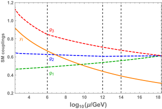
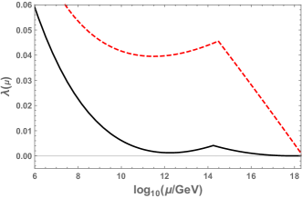
Figure 1: The SM gauge (dash line) and top Yukawa (solid line) couplings evolution in the Model I (panel (a)). The vector-like fermion $(Q_{x}+Q_{x}^{c})$ mass is set equal to 1 TeV. While masses for the particles $G_{x}(8,1,0)$ ($m_{8}=10^{6}$ GeV) and $W_{x}(1,3,0)$ ($M_{3}=1.13\times 10^{12}$) GeV are obtained from requiring that the gauge couplings should be unified at $2.43\times 10^{18}$ GeV. The scale for neutrino type I seesaw is taken at $10^{14}$ GeV. The panel (b) in Figure 1 displays evolution of the SM Higgs quartic coupling for Model I. The solid line stands for central values for $M_{h}=125.09$ GeV and $m_{t}=173.34$ GeV. The dashed lines corresponds to the $M_{h}=128.69$ GeV and $m_{t}=171.82$ GeV. The scale of x-axis is zoomed in order to show the behavior of $\lambda$ at high energy scale.

 

	121.49	123.29	125.09	126.89	128.69	Min.
171.82	-	$~{}2.0574\times 10^{14}~{}$	$~{}2.4043\times 10^{14}~{}$	$~{}2.7232\times 10^{14}~{}$	$~{}3.0305\times 10^{14}~{}$	122.02
172.58	-	-	$~{}2.1134\times 10^{14}~{}$	$~{}2.4644\times 10^{14}~{}$	$~{}2.7929\times 10^{14}~{}$	123.46
173.34	-	-	$~{}1.7786\times 10^{14}~{}$	$~{}2.1759\times 10^{14}~{}$	$~{}2.5334\times 10^{14}~{}$	124.89
174.10	-	-	-	$\;1.8375\times 10^{14}~{}$	$~{}2.2390\times 10^{14}~{}$	126.34
174.86	-	-	-	-	$~{}1.8977\times 10^{14}~{}$	127.79

Table 1: For Model I, dependence of right handed neutrino mass on the top and SM Higgs masses when gauge couplings are unified at $M_{U}=2.43\times 10^{18}~{}{\rm GeV}$. We use hyphen when there is no solution for given Higgs and top quark satisfying vacuum stability condition. For all solutions presented here, the SM Higgs quartic coupling is $O(10^{-6})$ at $M_{U}$ scale. The last column represents the lowest bounds of $M_{h}$ which satisfies vacuum stability bound for given top quark mass.

In Table 1, the dependence of right handed neutrino mass on the top and SM Higgs masses is shown when gauge couplings are unified at $M_{U}=2.43\times 10^{18}~{}{\rm GeV}$. The $m_{t}$ and $M_{h}$ are taken within two sigma uncertainty. We use hyphen when there is no solution for given SM Higgs and top quark satisfying vacuum stability condition. The last column represents the lowest bounds of $M_{h}$ which satisfies vacuum stability bound for given top quark mass. For all solutions presented in Table 1, the SM Higgs quartic coupling is $O(10^{-6})$ at $M_{U}$ scale. This will be very important once we consider Higgs inflation in next section.

In Figure 2(a), we display results for Model II with $m_{t}=173.34{\rm~{}GeV}$ and $m_{H}=125.06{\rm~{}GeV}$. The SM gauge (dash line) and top Yukawa (solid line) couplings evolution in present of vector-like fermions $(Q_{x}+Q_{x}^{c})$ and $(D_{x}+D_{x}^{c})$ at 1 TeV. The mass scale for $G_{x}(8,1,0)$ and $W_{x}(1,3,0)$ are the same and equal to $2.2\times 10^{12}$ GeV. In this case we have the gauge couplings unified at $2.43\times 10^{18}$ GeV. The neutrino type I seesaw scale is taken at $1.2\times 10^{14}$ GeV. The right panel (b) displays evolution of the SM Higgs quartic coupling for Model II. Different lines correspond to the different values of the SM Higgs and top quark mass at electroweak scale. The solid line stands for central values for $M_{h}=125.09$ GeV and $m_{t}=173.34$ GeV. The dotted line stands for $2\sigma$ theoretical and experimental bounds Patrignani:2016xqp $M_{h}=126.57$ GeV and $m_{t}=174.86$ GeV. The dashed lines correspond to the $M_{h}=128.69$ GeV and $m_{t}=171.82$ GeV. Behavior of RGE evolution of couplings are very similar what we had in Figure 1. Only significant difference is that additional vector-like fermions at TeV scale make more gradual evolution of SM Higgs quartic coupling compare to the Model I. This makes SM Higgs quartic coupling bigger when it reaches its minimal value around $10^{11}$ GeV scale, which allows us to have wider range for Top and Higgs masses and still have successful SM Higgs inflation.

As we can see from Figure 2(b), the solid line is way above zero during the RGE evolution. This makes the solution stable from radiative correction. Note the value of SM Higgs quartic coupling with central values of top and Higgs masses in Model II is significantly larger than the value in Model I.

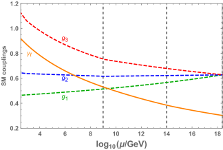
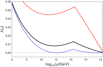
Figure 2: The SM gauge (dash line) and top Yukawa (solid line) couplings evolution in the Model II (panel (a)). The vector-like fermion $(Q_{x}+Q_{x}^{c})$ and $(D_{x}+D_{x}^{c})$ masses are set to 1 TeV. The mass scale for $G_{x}(8,1,0)$ and $W_{x}(1,3,0)$ particle masses are the same and equal to $1.2\times 10^{9}$ GeV. In this case we have the gauge couplings being unified at $2.43\times 10^{18}$ GeV. The neutrino type I seesaw scale is taken at $2.2\times 10^{14}$ GeV. The right panel (b) displays evolution of the SM Higgs quartic coupling for Model II. The solid line stands for central values for $M_{h}=125.09$ GeV and $m_{t}=173.34$ GeV. The dotted line stands for $M_{h}=126.57$ GeV and $m_{t}=174.86$ GeV. The dashed lines corresponds to the $M_{h}=128.69$ GeV and $m_{t}=171.82$ GeV. The scale of x-axis is zoomed in order to show the behavior of $\lambda$ at high energy scale.

	121.49	123.29	125.09	126.89	128.69	Min.
171.82	$~{}2.1146\times 10^{14}~{}$	$~{}2.4309\times 10^{14}~{}$	$~{}2.7292\times 10^{14}~{}$	$~{}3.0160\times 10^{14}~{}$	$~{}3.2959\times 10^{14}~{}$	121.49
172.58	-	$~{}2.1625\times 10^{14}~{}$	$~{}2.4858\times 10^{14}~{}$	$~{}2.7911\times 10^{14}~{}$	$~{}3.0851\times 10^{14}~{}$	122.28
173.34	-	-	$~{}2.2135\times 10^{14}~{}$	$~{}2.5440\times 10^{14}~{}$	$~{}2.8565\times 10^{14}~{}$	123.72
174.10	-	-	-	$~{}2.2679\times 10^{14}~{}$	$~{}2.6056\times 10^{14}~{}$	125.14
174.86	-	-	-	$~{}1.9513\times 10^{14}~{}$	$~{}2.3257\times 10^{14}~{}$	126.57

Table 2: For Model II, dependence of right handed neutrino mass on the top and SM Higgs masses when gauge couplings are unified at $M_{U}=2.43\times 10^{18}~{}{\rm GeV}$. We use hyphen when there is no solution for given Higgs and top quark satisfying vacuum stability condition. For all solutions presented here, the SM Higgs quartic coupling is $O(10^{-6})$ at $M_{U}$ scale. The last column represents the lowest bounds of $M_{h}$ which satisfies vacuum stability bound for given top quark mass.

In Table 2, the dependence of right handed neutrino mass on the top and SM Higgs masses is shown when gauge couplings are unified at $M_{U}=2.43\times 10^{18}~{}{\rm GeV}$. The $m_{t}$ and $M_{h}$ are taken within two sigma uncertainty. We use hyphen when there is no solution for given Higgs and top quark satisfying vacuum stability condition. The last column represents the lowest bounds of $M_{h}$ which satisfies vacuum stability bound for given top quark mass. For all solutions presented in Table 1, the SM Higgs quartic coupling is $O(10^{-6})$ at $M_{U}$ scale. This will be very important once we consider Higgs inflation in next section. Compared with Model I, the allowed range for $m_{t}$ and $M_{h}$ parameter space is larger in Model II.

IV Higgs Inflation

Next, we consider the Higgs inflation by introducing a non-minimal coupling between the Higgs doublet and gravity. In the Jordan frame, the action is

$$S_{J}=\int d^{4}x\;\sqrt{-g}\left[-(\frac{1}{2}+\xi H^{+}H)R+(D_{\mu}H)^{+}(D_{\mu}H)-\frac{1}{2}\lambda(H^{+}H-\frac{v^{2}}{2})^{2}\right]~{},~{}\,$$ (2)

where the reduced Planck scale $M_{{\rm Pl}}$ is set to be $1$, and $H=(0,v+\phi)/\sqrt{2}$ is the Higgs doublet in the unitary gauge. The physical Higgs field $\phi$ is taken to be the inflaton.

The RGE improved effective inflaton potential is

$$V(\phi)=\frac{\lambda(\phi)}{8}\phi^{4}$$ (3)

with $\lambda(\phi)$ the solution of the RGE for the Higgs coupling. In the Einstein frame with a canonical gravity sector, the theory is described by a new inflaton field $\sigma$ that has a canonical kinetic term. The relation between $\sigma$ and $\phi$ is

$$\left(\frac{\mathrm{d}\sigma}{\mathrm{d}\phi}\right)^{-2}=\dfrac{(1+\xi\phi^{2})^{2}}{1+(6\xi+1)\xi\phi^{2}}~{}.$$ (4)

The action becomes

$$S_{E}=\int d^{4}x\;\sqrt{-g_{E}}\left[-\frac{1}{2}R_{E}+\frac{1}{2}(\partial\sigma)^{2}-V_{E}(\phi(\sigma))\right]\;,$$ (5)

where

$$V_{E}(\phi)=\frac{\lambda(\phi)\phi^{4}}{8\left(\xi\phi^{2}+1\right)^{2}}\;.$$ (6)

The inflationary slow-roll parameters in terms of $\phi$ are expressed as

$$\epsilon(\phi) = \frac{M_{Pl}^{2}}{2}\left(\dfrac{V^{\prime}_{E}}{V_{E}\sigma^{\prime}}\right),$$ (7)

$$\eta(\phi) = M_{Pl}^{2}\left[\dfrac{V^{\prime\prime}_{E}}{V_{E}(\sigma^{\prime})^{2}}-\dfrac{V^{\prime}_{E}\sigma^{\prime\prime}}{V_{E}(\sigma^{\prime})^{3}}\right],$$ (8)

$$\zeta(\phi) = M_{Pl}^{4}\left(\dfrac{V^{\prime}_{E}}{V_{E}\sigma^{\prime}}\right)\left(\dfrac{V^{\prime\prime\prime}_{E}}{V_{E}(\sigma^{\prime})^{3}}-3\dfrac{V^{\prime\prime}_{E}\sigma^{\prime\prime}}{V_{E}(\sigma^{\prime})^{4}}+3\dfrac{V^{\prime}_{E}(\sigma^{\prime\prime})^{2}}{V_{E}(\sigma^{\prime})^{5}}-\dfrac{V^{\prime}_{E}\sigma^{\prime\prime\prime}}{V_{E}(\sigma^{\prime})^{4}}\right),$$ (9)

where the prime denotes a derivative with respect to $\phi$, while $\lambda(\phi)$ is taken as $\lambda(\phi_{0})$. The scalar spectral index, tensor-to-scalar ratio, running of the scalar spectral index, and power spectrum Lyth:1998xn-1 are respectively

$$n_{s} = 1-6\epsilon+2\eta+2\left[\frac{1}{3}\eta^{2}-\left(\frac{5}{3}+12C\right)\epsilon^{2}+(8C-1)\epsilon\eta-(C-\frac{1}{3})\zeta\right]~{},$$ (10)

$$r = 16\epsilon\left[1+\frac{2}{3}(3C-1)(2\epsilon-\eta)\right]~{},$$ (11)

$$\alpha_{s} = \frac{\mathrm{d}n_{s}}{\mathrm{d}\ln k}=16\epsilon\eta-24\epsilon^{2}-2\zeta~{},~{}$$ (12)

$$P_{s} = \dfrac{V_{E}}{24\pi^{2}\epsilon},$$ (13)

where $C=-2+\ln 2+\gamma\simeq-0.7296$ with $\gamma$ the Euler–Mascheroni constant. Here, we also considered the second-order corrections, which will give extra contributions of $\delta n_{s}\sim 0.001$ and $\delta r\sim-1\times 10^{-4}$. The e-folding number is given by

$$N = \frac{1}{M_{{\rm Pl}}}\int_{\phi_{e}}^{\phi_{0}}\dfrac{\mathrm{d}\phi}{\sqrt{2\epsilon(\phi)}}\left(\dfrac{\mathrm{d}\sigma}{\mathrm{d}\phi}\right)$$ (14)

and the inflation ends once $\epsilon(\phi_{e})$ or $|\eta(\phi_{e})|$ reaches 1.

In the following numerical discussions, we shall find that inflation always ends when $\epsilon=1$ in Models I and II. So let us study the corresponding constraint on $\xi$. For $\epsilon(\phi_{e})=1$, there are two positive roots and two negative roots for $\phi_{e}$:

$$\phi_{1}=\frac{4}{\sqrt{1+\sqrt{(8\xi+1)(24\xi+1)}}}~{},~{}$$ (15)

$$\phi_{2}=\frac{4}{\sqrt{1-\sqrt{(8\xi+1)(24\xi+1)}}}~{},~{}$$ (16)

$$\phi_{3}=-\frac{4}{\sqrt{1+\sqrt{(8\xi+1)(24\xi+1)}}}~{},~{}$$ (17)

$$\phi_{4}=-\frac{4}{\sqrt{1-\sqrt{(8\xi+1)(24\xi+1)}}}.$$ (18)

Because we require both $\phi>0$ and $\xi>0$, Eq. (15) is the only physical solution. Let us study the possible value of $\xi$ in the following

(1) Assume that $\xi$ locates in the range of $0<\xi\leq 1$, we obtain $\phi_{e}\geq 2\sqrt{\frac{2}{7}}~{}M_{{\rm Pl}}$ from Eq. (15). And then inflation ends above the reduced Planck scale, Thus, we can have $0<\xi\leq 1$ only for the trans-Planckian inflation.

(2) To satisfy the condition $0<\phi_{e}<M_{{\rm Pl}}$, we find that $\xi$ can only locate in the ranges of $\xi>1$ or $\xi<-\frac{7}{6}$. With $\xi>1$ and $\phi_{0}>\phi_{e}$, the number of e-folding is

$$N=\frac{1}{8}\left(6\log\left(\frac{1+\xi\phi_{e}^{2}}{1+\xi\phi_{0}^{2}}\right)+(1+6\xi)(\phi_{0}-\phi_{e})(\phi_{0}+\phi_{e})\right)$$ (19)

With $N$ fixed, Eq. (19) is actually a functional relation between $\xi$ and $\phi_{0}$. We present $\xi$ versus $\phi_{0}$ with the fixed $N$ in Fig. 3. To have $\phi_{0}\leq M_{{\rm Pl}}$, we obtain $\xi\geq 71.16$ for $N=50$ and $\xi\geq 84.67$ for $N=60$ from Fig. 3.

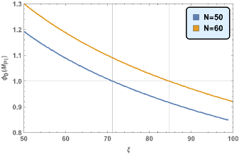
Figure 3: The gray lines is corresponding to $\xi=71.16$ with $N=50$ and $\xi=84.67$ with $N=60$.

In short, for Higgs inflation taking place below the reduced Planck scale, i.e., the sub-Planckian inflation, there is a lower bound on $\xi$, which is $71.16$ for $N=50$ and $84.67$ for $N=60$. Especially, it is impossible to get $0<\xi\leq 1$. This conclusion is model independent as long as the Higgs-gravity coupling is taken to be in Eq. (2).

V Numerical Study for Inflation

We will discuss the numerical results for the inflationary observables as our predictions, which can fit the current experimental data. We define the precise gauge coupling unification condition as $\alpha_{1}^{-1}\equiv(\alpha_{2}^{-1}+\alpha_{3}^{-1})/2$, as well as consider the string scale unification with $M_{U}=3\times 10^{17}{\rm~{}GeV}$ and the reduced Planck scale unification with $M_{U}=M_{{\rm Pl}}=2.43\times 10^{18}{\rm~{}GeV}$.

For a fixed $N=50$ and 60, we find that the inflationary predictions or observables can be consistent with all the current experimental constraints from the Planck, Baryon Acoustic Oscillations (BAO), and BICEP2/Keck Array data, etc Ade:2015lrj ; Array:2015xqh . And the couplings $\xi$ can be adjusted to realize the observed power spectrum $P_{s}=2.20\times 10^{-9}$. In particular, we find that inflation always ends when $\epsilon=1$ in our models. For numerical results, we present some concrete benchmark points for Model I in Tables 3 as well as for Model II in Tables 4. To achieve the gauge coupling unification at the reduced Planck scale, we find that $M_{8}\sim 1.0\times 10^{6}~{}{\rm GeV}$ and $M_{3}\sim 1.0\times 10^{12}~{}{\rm GeV}$ in Model I, as well as $M_{8}\sim 1.25\times 10^{9}~{}{\rm GeV}$ and $M_{3}\sim 1.24\times 10^{9}~{}{\rm GeV}$ in Model II. Thus, we have $M_{8}\simeq M_{3}$ in Model II, which makes it much more interesting. Neglecting $G_{x}$ and $W_{x}$ in Model II, we do have gauge coupling unification around $2\times 10^{16}$ GeV Chen:2017rpn . Thus, introducing the $SU(3)_{C}$ and $SU(2)_{L}$ adjoint fermions/chiral superfields with the similar intermediate-scale mass in the GUTs, supersymmetric GUTs and string models, we can lift the tradition GUT scale to the string scale or reduced Planck scale in general, which will be very important at least in the string model building! Moreover, the scalar spectral indices are almost the same and they are around 0.9626 and 0.9685 respectively for $N=50$ and $N=60$, the tensor-to-scalar ratios are at the order of $10^{-3}$, and the running of the scalar spectral index is negative and at the order of $10^{-6}$. In particular, with some fine-tuning of the input parameters, we can obtain that $\lambda(\phi_{0})$ is at the order of $10^{-6}$, and then $\xi$s are close to their lower bounds around $\xi\sim 71-84$, which are given in Tables 3 and 4. In short, we indeed solve the $\xi$ problem in the Higgs inflation. In Tables 1 - 6, the values at the center of both tables is the Seesaw scale $M_{R}$ adopted to meet requirements. $\lambda$ should be as small as possible for the purpose of Higgs inflation happening at inflation scale but still above zero to solve the stability problem. The precision of $M_{R}$ shown in the Tables 1 - 6 is due to the small $\zeta$ in our models.  1 and 2 are the allowed range of paramters of $m_{t}$ and $M_{h}$ in model I when the unification is around the reduced Planck scale. Tables 5and 6 are for model II when the unification happens at the string scale.

To understand our numerical results with small $\xi$ close to its lower bound, let us study it in more details. The scalar power spectrum amplitude is given by

$$P_{s}(\xi,\phi_{0}) = \dfrac{1}{24\pi^{2}}\dfrac{V(\xi,\phi_{0})}{\epsilon(\xi,\phi_{0})}$$ (20)

$$= \dfrac{\lambda(\phi_{0})\phi_{0}^{6}}{1536\pi^{2}}\times\dfrac{1+\xi(1+6\xi)\phi_{0}^{2}}{(1+\xi\phi_{0}^{2})^{2}},$$

where the Higgs coupling $\lambda(\phi_{0})$ also depends on the parameters involved in the RGE evolution, $\lambda(\phi_{0})=\lambda(\phi_{0}|m_{t},M_{R},M_{8},M_{3},M_{U})$. With $\xi$ given and $N=50$ fixed, $\phi_{0}$ is determined, so we actually have $\phi_{0}=\phi_{0}(\xi)$. The relations between $(\xi,\phi_{0},P_{s})$ are plotted as the functions $\phi_{0}=\phi_{0}(\xi)$, $P_{s}=P_{s}(\phi_{0}|m_{t},M_{R},M_{8},M_{3},M_{U})$, and $P_{s}=P_{s}(\xi|m_{t},M_{R},M_{8},M_{3},M_{U})$ for Model II in Figs. 4, where $(m_{t},M_{R},M_{8},M_{3},M_{U})$ are taken to be $(173.34,1.7786\times 10^{14},1.25\times 10^{9},1.24\times 10^{9},2.43\times 10^{18})$ GeV. As we can see from these figures, $\phi_{0}=\phi_{0}(\xi)$ is an input parameter independent function, however, $\phi_{0}$ decreases when $\xi$ increases. On the other hand, $P_{s}=P_{s}(\phi_{0}|m_{t},M_{R},M_{8},M_{3},M_{U})$ and $P_{s}=P_{s}(\xi|m_{t},M_{R},M_{8},M_{3},M_{U})$ delicately depend on the selected input parameters. With little changes in $m_{t}$ and $M_{R}$, the functions with the local maximum become the functions with the local minimum. The gray lines in Fig. 4 give the constraint of the correct power spectrum $P_{s}=2.20\times 10^{-9}$. Thus, we show explicitly that there are two viable regions in the $P_{s}$ versus $\phi_{0}(M_{{\rm Pl}})$ and $P_{s}$ versus $\xi$ planes, which give the observed power spectrum. One kind of viable regions has small $\xi\subset(70-86)$ and large $\phi_{0}\sim M_{{\rm Pl}}$, and the benchmark points are given in Tables 3 and 4. In both of our models, we can indeed obtain $\xi$ around $70-80$, which is almost the minimum $\xi$ that can be realized. And then the $\xi$ problem is indeed solved.

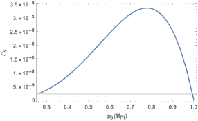
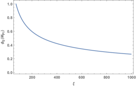
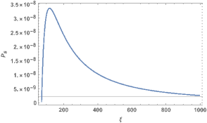
Figure 4: The relation between $P_{s}$, $\phi_{0}$ and $\xi$ for Model II with $m_{t}=173.34{\rm~{}GeV}$,$M_{h}=125.09{\rm~{}GeV}$ and $M_{U}=2.43\times 10^{18}{\rm~{}GeV}$. The e-folding number is fixed at 50.

 

 

 

 

 

 

	$m_{t}=173.34$,$M_{h}=125.09$,$M_{R}=1.7786\times 10^{14}$, $M_{8}=1.\times 10^{6}$, $M_{3}=1.13\times 10^{12}$, $M_{U}=2.43\times 10^{18}$
N	$\xi$	$\phi_{0}({\rm M_{Pl})}$	$\phi_{e}({\rm M_{Pl})}$	$n_{s}$	$r(10^{-3})$	$\alpha(10^{-4})$	$\lambda(\phi_{0})$	$\lambda(M_{U})$
50	145.8	0.6991	0.0889	0.9626	4.03	-7.48	$2.39\times 10^{-5}$	$5.36\times 10^{-5}$
60	173.7	0.6985	0.0815	0.9685	2.87	-5.23	$2.39\times 10^{-5}$	$5.36\times 10^{-5}$
	$m_{t}=172.58$,$M_{h}=126.89$,$M_{R}=2.1286\times 10^{14}$, $M_{8}=2.3\times 10^{9}$, $M_{3}=2.1\times 10^{14}$, $M_{U}=3.0\times 10^{17}$
N	$\xi$	$\phi_{0}({\rm M_{Pl})}$	$\phi_{e}({\rm M_{Pl})}$	$n_{s}$	$r(10^{-3})$	$\alpha(10^{-4})$	$\lambda(\phi_{0})$	$\lambda(M_{U})$
50	73.05	0.98706	0.1256	0.9626	4.03	-7.48	$6.01\times 10^{-6}$	$3.29\times 10^{-3}$
60	86.91	0.98707	0.1152	0.9685	2.87	-5.23	$6.00\times 10^{-6}$	$3.29\times 10^{-3}$
	$m_{t}=172.58$,$M_{h}=126.89$, $M_{R}=2.4644\times 10^{14}$, $M_{8}=1.07\times 10^{6}$, $M_{3}=1.\times 10^{12}$, $M_{U}=2.43\times 10^{18}$
N	$\xi$	$\phi_{0}({\rm M_{Pl})}$	$\phi_{e}({\rm M_{Pl})}$	$n_{s}$	$r(10^{-3})$	$\alpha(10^{-4})$	$\lambda(\phi_{0})$	$\lambda(M_{U})$
50	71.237	0.9995	0.1272	0.9626	4.03	-7.48	$5.72\times 10^{-6}$	$2.11\times 10^{-6}$
60	84.763	0.9995	0.1166	0.9685	2.87	-5.23	$5.69\times 10^{-6}$	$2.11\times 10^{-6}$
	$m_{t}=174.10$,$M_{h}=126.89$, $M_{R}=1.8374\times 10^{14}$, $M_{8}=1.\times 10^{6}$, $M_{3}=1.12\times 10^{12}$, $M_{U}=2.43\times 10^{18}$
N	$\xi$	$\phi_{0}({\rm M_{Pl})}$	$\phi_{e}({\rm M_{Pl})}$	$n_{s}$	$r(10^{-3})$	$\alpha(10^{-4})$	$\lambda(\phi_{0})$	$\lambda(M_{U})$
50	72.78	0.9889	0.1258	0.9626	4.03	-7.48	$5.97\times 10^{-6}$	$4.72\times 10^{-6}$
60	86.53	0.9892	0.1154	0.9685	2.87	-5.23	$5.93\times 10^{-6}$	$4.72\times 10^{-6}$

Table 3: The benchmark points with small $\xi$ in Model I for $N=50$ and 60, where the mass unit is GeV.

	$m_{t}=173.34$,$M_{h}=125.09$,$M_{R}=1.9963\times 10^{14}$, $M_{8}=1.02\times 10^{12}$,$M_{3}=1.02\times 10^{12}$,$M_{U}=3.0\times 10^{17}$
N	$\xi$	$\phi_{0}({\rm M_{Pl})}$	$\phi_{e}({\rm M_{Pl})}$	$n_{s}$	$r(10^{-3})$	$\alpha(10^{-4})$	$\lambda(\phi_{0})$	$\lambda(M_{U})$
50	74.442	0.9778	0.1244	0.9626	4.03	-7.48	$6.24\times 10^{-6}$	$1.41\times 10^{-3}$
60	88.558	0.9779	0.1141	0.9685	2.87	-5.23	$6.21\times 10^{-6}$	$1.41\times 10^{-3}$
	$m_{t}=173.34$,$M_{h}=125.09$,$M_{R}=2.2135\times 10^{14}$,$M_{8}=1.24\times 10^{9}$,$M_{3}=1.24\times 10^{9}$,$M_{U}=2.43\times 10^{18}$
N	$\xi$	$\phi_{0}({\rm M_{Pl})}$	$\phi_{e}({\rm M_{Pl})}$	$n_{s}$	$r(10^{-3})$	$\alpha(10^{-4})$	$\lambda(\phi_{0})$	$\lambda(M_{U})$
50	71.923	0.9947	0.1266	0.9626	4.03	-7.48	$5.83\times 10^{-6}$	$1.14\times 10^{-6}$
60	85.566	0.9947	0.1160	0.9685	2.87	-5.23	$5.80\times 10^{-5}$	$1.14\times 10^{-6}$
	$m_{t}=172.58$,$M_{h}=126.89$,$M_{R}=2.6295\times 10^{14}$,$M_{8}=1.02\times 10^{12}$,$M_{3}=1.02\times 10^{12}$,$M_{U}=3.0\times 10^{17}$
N	$\xi$	$\phi_{0}({\rm M_{Pl})}$	$\phi_{e}({\rm M_{Pl})}$	$n_{s}$	$r(10^{-3})$	$\alpha(10^{-4})$	$\lambda(\phi_{0})$	$\lambda(M_{U})$
50	76.157	0.9668	0.1230	0.9625	4.03	-7.48	$6.53\times 10^{-5}$	$6.58\times 10^{-3}$
60	87.223	0.9853	0.1150	0.9685	2.87	-5.23	$6.02\times 10^{-6}$	$6.58\times 10^{-3}$
	$m_{t}=172.58$,$M_{h}=126.89$,$M_{R}=2.7911\times 10^{14}$,$M_{8}=1.24\times 10^{9}$,$M_{3}=1.24\times 10^{9}$,$M_{U}=2.43\times 10^{18}$
N	$\xi$	$\phi_{0}({\rm M_{Pl})}$	$\phi_{e}({\rm M_{Pl})}$	$n_{s}$	$r(10^{-3})$	$\alpha(10^{-4})$	$\lambda(\phi_{0})$	$\lambda(M_{U})$
50	71.383	0.9985	0.1270	0.9625	4.03	-7.48	$5.74\times 10^{-6}$	$1.05\times 10^{-6}$
60	84.927	0.9985	0.1165	0.9685	2.87	-5.23	$5.71\times 10^{-6}$	$1.05\times 10^{-6}$
	$m_{t}=174.10$,$M_{h}=126.89$,$M_{R}=2.0542\times 10^{14}$,$M_{8}=1.02\times 10^{12}$,$M_{3}=1.02\times 10^{12}$,$M_{U}=3.0\times 10^{17}$
N	$\xi$	$\phi_{0}({\rm M_{Pl})}$	$\phi_{e}({\rm M_{Pl})}$	$n_{s}$	$r(10^{-3})$	$\alpha(10^{-4})$	$\lambda(\phi_{0})$	$\lambda(M_{U})$
50	73.773	0.9822	0.1250	0.9626	4.03	-7.48	$6.13\times 10^{-6}$	$1.89\times 10^{-3}$
60	87.765	0.9823	0.1146	0.9685	2.87	-5.23	$6.10\times 10^{-6}$	$1.89\times 10^{-3}$
	$m_{t}=174.10$,$M_{h}=126.89$,$M_{R}=2.2679\times 10^{14}$,$M_{8}=1.24\times 10^{9}$,$M_{3}=1.24\times 10^{9}$,$M_{U}=2.43\times 10^{18}$
N	$\xi$	$\phi_{0}({\rm M_{Pl})}$	$\phi_{e}({\rm M_{Pl})}$	$n_{s}$	$r(10^{-3})$	$\alpha(10^{-4})$	$\lambda(\phi_{0})$	$\lambda(M_{U})$
50	71.875	0.9951	0.1266	0.9626	4.03	-7.48	$5.81\times 10^{-6}$	$3.95\times 10^{-7}$
60	85.510	0.9951	0.1161	0.9685	2.87	-5.23	$5.79\times 10^{-6}$	$3.95\times 10^{-7}$

Table 4: The benchmark points with small $\xi$ in Model II for $N=50$ and 60, where the masses are in GeV.

	121.49	123.29	125.09	126.89	128.69	Mini
171.82	-	$~{}1.6510\times 10^{14}~{}$	$~{}2.0658\times 10^{14}~{}$	$~{}2.4343\times 10^{14}~{}$	$~{}2.7766\times 10^{14}~{}$	122.70
172.58	-	-	$~{}1.7088\times 10^{14}~{}$	$~{}2.1288\times 10^{14}~{}$	$~{}2.5041\times 10^{14}~{}$	124.17
173.34	-	-	-	$~{}1.7688\times 10^{14}~{}$	$~{}2.1950\times 10^{14}~{}$	125.65
174.10	-	-	-	-	$~{}2.2390\times 10^{14}~{}$	127.12
174.86	-	-	-	-	$~{}1.1929\times 10^{14}~{}$	128.60

Table 5: For Model I, dependence of right handed neutrino mass on the top and SM Higgs masses when gauge couplings are unified at $M_{U}=3.0\times 10^{17}~{}{\rm GeV}$. We use hyphen when there is no solution for given Higgs and top quark satisfying vacuum stability condition. For all solutions presented here the Higgs quartic coupling is $O(10^{-6})$ at $M_{U}$ scale. The last column represents the lowest bounds of $M_{h}$ which satisfies vacuum stability bound for give top quark mass.

	121.49	123.29	125.09	126.89	128.69	Mini
171.82	$~{}1.8920\times 10^{14}~{}$	$~{}2.2502\times 10^{14}~{}$	$~{}2.5649\times 10^{14}~{}$	$~{}2.8919\times 10^{14}~{}$	$~{}3.1930\times 10^{14}~{}$	121.49
172.58	-	$~{}1.9418\times 10^{14}~{}$	$~{}2.2992\times 10^{14}~{}$	$~{}2.6295\times 10^{14}~{}$	$~{}2.9430\times 10^{14}~{}$	122.42
173.34	-	-	$~{}1.9963\times 10^{14}~{}$	$~{}2.3604\times 10^{14}~{}$	$~{}2.6976\times 10^{14}~{}$	123.86
174.10	-	-	-	$~{}2.0542\times 10^{14}~{}$	$~{}2.4251\times 10^{14}~{}$	125.30
174.86	-	-	-	$~{}1.6689\times 10^{14}~{}$	$~{}2.1157\times 10^{14}~{}$	126.75

Table 6: For Model II, dependence of right handed neutrino mass on the top and SM Higgs masses when gauge couplings are unified at $M_{U}=3.0\times 10^{17}~{}{\rm GeV}$. We use hyphen when there is no solution for given Higgs and top quark satisfying vacuum stability condition. For all solutions presented here the Higgs quartic coupling is $O(10^{-6})$ at $M_{U}$ scale. The last column represents the lowest bounds of $M_{h}$ which satisfies vacuum stability bound for give top quark mass.

VI Conclusion

We have studied two non-supersymmetric models with gauge couplings unification. In these scenarios, the so-called critical Higgs inflation ($\xi<100$) could be naturally realized and the SM vacuum stability problem can be solved. In order to achieve the gauge coupling unification around the string scale, we introduce new particles at TeV and intermediate scales. Also, we employed the Type I seesaw mechanism explaining the tiny neutrino masses. We have shown that, by choosing the Seesaw scale, we can control the SM Higgs quartic coupling at the inflation scale.

We present a few benchmark points where we show that the scalar spectral indices are around 0.9626 and 0.9685 for the number of e-folding $N=50$ and $N=60$ respectively. The tensor-to-scalar ratios are order of $10^{-3}$. The running of the scalar spectral index is negative and is order of $10^{-4}$.

Appendix A The RGEs in the SM

For three standard model (SM) gauge couplings, we employ the two-loop RGEs AMALDO1992374 ; Barger:1992ac

$$\dfrac{\mathrm{d}g_{i}}{\mathrm{d}\ln\mu} = \dfrac{g_{i}}{16\pi^{2}}\left[b_{i}^{SM}g_{i}^{2}+\dfrac{1}{16\pi^{2}}\left(\sum_{j=1}^{3}b_{ij}^{SM}g_{i}^{2}g_{j}^{2}-C_{i}^{t}g_{i}^{2}y_{t}^{2}\right)\right],$$ (21)

where $g_{i}~{}(i=1,2,3)$ are the SM gauge couplings, $y_{t}$ is the top quark Yukawa coupling, and

$$b_{i}^{SM}=\left(\frac{41}{9},-\frac{19}{6},-7\right),~{}b_{ij}^{SM}=\begin{pmatrix}\frac{199}{50}&\frac{27}{10}&\frac{44}{5}\\ \frac{9}{10}&\frac{35}{6}&12\\ \frac{11}{10}&\frac{9}{2}&-26\end{pmatrix},~{}C_{i}^{t}=\left(\frac{17}{10},\frac{3}{2},2\right).$$ (22)

The RGE for the top quark Yukawa coupling is

$$\dfrac{\mathrm{d}y_{t}}{\mathrm{d}\ln\mu} = y_{t}\left(\frac{1}{16\pi^{2}}\beta_{t}^{(1)}+\dfrac{1}{(16\pi^{2})^{2}}\beta_{t}^{(2)}\right)$$ (23)

with the one-loop and two-loop contributions given by

$$\beta_{t}^{(1)} = -\sum c_{i}^{SM}g_{i}^{2}+\frac{3}{2}y_{t}^{2}+Y_{2},$$ (24)

$$\beta_{t}^{(2)} = \frac{1187g_{1}^{4}}{600}-\frac{23g_{2}^{4}}{4}-108g_{3}^{4}-\frac{3}{20}g_{2}^{2}g_{1}^{2}+\frac{19}{15}g_{3}^{2}g_{1}^{2}+9g_{2}^{2}g_{3}^{2}$$ (25)

$$+y_{t}^{2}\left(\frac{223}{80}g_{1}^{2}+\frac{135}{16}g_{2}^{2}+16g_{3}^{2}\right)$$

$$+\frac{5}{2}Y_{4}-6\lambda y_{t}^{2}+\frac{3}{2}y_{t}^{4}-\frac{9}{4}Y_{2}y_{t}^{2}-\chi_{4}+\frac{3}{2}\lambda^{2},$$

where $Y_{2}=3y_{t}^{2}$, $Y_{4}=\sum_{i=1}^{3}c_{i}^{SM}g_{i}^{2}y_{t}^{2}$, $\chi=\frac{27}{4}y_{t}^{4}$, and $c_{i}^{SM}=\left(\frac{17}{20},\frac{9}{4},8\right)$. The RGE for the Higgs boson quartic coupling is

$$\dfrac{\mathrm{d}\lambda}{\mathrm{d}\ln\mu} = \frac{1}{16\pi^{2}}\beta_{\lambda}^{(1)}+\dfrac{1}{(16\pi^{2})^{2}}\beta_{\lambda}^{(2)},$$ (26)

where the one-loop and two-loop contributions are

$$\beta_{\lambda}^{(1)} = 12\lambda^{2}+12y_{t}^{2}\lambda-12y_{t}^{4}-\left(\frac{9}{5}g_{1}^{2}+9g_{2}^{2}\right)\lambda+$$ (27)

$$\frac{9}{4}\left(\frac{3}{25}g_{1}^{4}+\frac{2}{5}g_{1}^{2}g_{2}^{2}+g_{2}^{4}\right)$$

$$\beta_{\lambda}^{(2)} = -78\lambda^{3}+18\left(\frac{3}{5}g_{1}^{2}+3g_{2}^{2}\right)\lambda^{2}-\left(\frac{73}{8}g_{2}^{4}-\frac{117}{20}g_{1}^{2}g_{2}^{2}-\frac{1887}{200}g_{1}^{4}\right)\lambda-3\lambda y_{t}^{4}$$ (28)

$$+\frac{305}{8}g_{2}^{6}-\frac{867}{120}g_{1}^{2}g_{2}^{4}-\frac{1677}{200}g_{1}^{4}g_{2}^{2}-\frac{3411}{1000}g_{1}^{6}-64g_{3}^{2}y_{t}^{4}-\frac{16}{5}g_{1}^{2}y_{t}^{4}-\frac{9}{2}g_{2}^{4}y_{t}^{2}$$

$$+10\lambda y_{t}^{2}\left(\frac{17}{20}g_{1}^{2}+\frac{9}{4}g_{2}^{2}+8g_{3}^{2}\right)-\frac{3}{5}g_{1}^{2}y_{t}^{2}\left(\frac{57}{10}g_{1}^{2}-21g_{2}^{2}\right)$$

$$-72\lambda^{2}y_{t}^{2}+60y_{t}^{6}~{}.~{}\,$$

Appendix B Additional contribution to the SM RGEs

The one-loop contributions to the beta function coefficients from the new particles are  GCU ; Barger:2007qb

$$\Delta b^{Q_{x}+Q_{x}^{c}}=\left(\frac{2}{15},2,\frac{4}{3}\right)~{},~{}~{}~{}\Delta b^{D_{x}+D_{x}^{c}}=\left(\frac{4}{15},0,\frac{2}{3}\right)~{},~{}$$

$$\Delta b^{G_{x}}=(0,0,2)~{},~{}~{}~{}\Delta b^{W_{x}}=\left(0,\frac{4}{3},0\right)~{},~{}$$

and the two-loop contributions are

$$\Delta B^{Q_{x}+Q_{x}^{c}}=\left(\begin{array}[]{ccc}\frac{1}{150}&\frac{3}{10}&\frac{8}{15}\\ \frac{1}{10}&\frac{49}{2}&8\\ \frac{1}{15}&3&\frac{76}{3}\end{array}\right) \Delta B^{D_{x}+D_{x}^{c}}=\left(\begin{array}[]{ccc}\frac{4}{75}&0&\frac{16}{15}\\ 0&0&0\\ \frac{2}{15}&0&\frac{38}{3}\end{array}\right),$$ , (35)

$$\Delta B^{G_{x}}=\left(\begin{array}[]{ccc}0&0&0\\ 0&0&0\\ 0&0&48\end{array}\right) \Delta B^{W_{x}}=\left(\begin{array}[]{ccc}0&0&0\\ 0&\frac{64}{3}&0\\ 0&0&0\end{array}\right).$$ , (42)

The mass scales of the vector-like fermions $(Q_{x},~{}Q_{x}^{c})$ and $(D_{x},~{}D_{x}^{c})$ are set to be $M_{V}=1~{}{\rm TeV}$, and we denote the masses of $G_{x}$ and $W_{x}$ as $M_{8}$ and $M_{3}$, respectively, which will be chosen at the intermediate scales. When renormalization scale $\mu$ is larger than $M_{V}$, $M_{3}$, or $M_{8}$, the contributions of the corresponding particles should be taken into account.

Appendix C Type I Seesaw Mechanism

Here we present additional one-loop contributions to the various beta function coefficients having Type I seesaw mechanism for neutrino masses. We define

$$S_{\nu}=Y_{\nu}^{\dagger}Y_{\nu}=Y_{\nu}^{T}Y_{\nu}=-\dfrac{2M_{R}}{v^{2}}M_{\nu},$$

then additional one loop contribution to the top Yukawa and Higgs quartic couplings are the following

$$\delta\beta_{t}^{(1)}=\mathrm{tr}[S_{\nu}],$$ (43)

$$\delta\beta_{\lambda}^{(1)}=4\mathrm{tr}[S_{\nu}]\lambda-4\mathrm{tr}[S_{\nu}^{2}]~{}.~{}\,$$ (44)

Above the scale of right handed neutrino we have the following one loop RGE for $S_{\nu}$

$$\dfrac{\mathrm{d}S_{\nu}}{\mathrm{d}\ln\mu}=\dfrac{S_{\nu}}{16\pi^{2}}\left[6y_{t}^{2}+2\mathrm{tr}[S_{\nu}]-\left(\frac{9}{10}g_{1}^{2}+\frac{9}{2}g_{2}^{2}\right)+3S_{\nu}\right]\;.$$ (45)

Appendix D Phenomenological constraints and scanning procedure

With $M_{V}$, $M_{3}$, $M_{8}$ and $M_{R}$ fixed, we solve the RGEs to get the evolution of the SM Higgs quartic coupling from $M_{Z}$ to $M_{{\rm String}}=3\times 10^{17}~{}$GeV or $M_{{\rm Pl}}=2.43\times 10^{18}~{}{\rm GeV}$ which is the unification scale in our models. We integrate the SM gauge coupling RGEs first in Eq. (21) with $y_{t}$ from $M_{Z}$ to $m_{t}$ to determine the initial value of the top quark Yukawa coupling $y_{t}(m_{t})$. The running top quark mass $m_{t}$ gets one-loop and two-loop QCD corrections and also the one-loop electroweak one-loop correction. To solve the RGEs, we use the boundary conditions at $M_{Z}$ given by

$$g_{1}(M_{Z})=\sqrt{\frac{5}{3}}\dfrac{g_{{\rm em}}}{\cos\theta_{W}}~{},\;g(M_{Z})=\dfrac{g_{{\rm em}}}{\sin\theta_{W}}~{},\;g(M_{Z})=\sqrt{4\pi\alpha_{3}}\;,\;y_{t}(m_{t})=\dfrac{\sqrt{2}M_{t}(m_{t})}{v},$$ (46)

We then integrate the RGEs for $(g_{i},y_{t},\lambda)$ from $M_{Z}$ to the scales of vector-like fermions $M_{V}$, $M_{3}$, $M_{8}$ and to the Seesaw scale $M_{R}$ and continue to integrate the RGEs for $(g_{i},y_{t},\lambda,S_{\nu})$ from $M_{R}$ to $M_{String}/M_{Pl}$.

References

- (1) G. Aad et al. [ATLAS Collaboration], Phys. Lett. B 716, 1 (2012) [arXiv:1207.7214 [hep-ex]].
- (2) S. Chatrchyan et al. [CMS Collaboration], Phys. Lett. B 716, 30 (2012) [arXiv:1207.7235 [hep-ex]].
- (3) https://twiki.cern.ch/twiki/bin/view/AtlasPublic/HiggsPublicResults; https://twiki.cern.ch/twiki/bin/view/CMSPublic/PhysicsResultsHIG.
- (4) See for instance, D. Buttazzo, G. Degrassi, P. P. Giardino, G. F. Giudice, F. Sala, A. Salvio and A. Strumia, JHEP 1312, 089 (2013) [arXiv:1307.3536 [hep-ph]]. Mod. Phys. Lett. A 28, 1330002 (2013) [arXiv:1301.5812 [hep-ph]].
- (5) A. A. Starobinsky, Phys. Lett. B 91, 99 (1980); A. H. Guth, Phys. Rev. D 23, 347 (1981); A. D. Linde, Phys. Lett. B 108, 389 (1982); A. Albrecht and P. J. Steinhardt, Phys. Rev. Lett. 48, 1220 (1982).
- (6) F. L. Bezrukov and M. Shaposhnikov, Phys. Lett. B 659, 703 (2008) [arXiv:0710.3755 [hep-th]]; A. O. Barvinsky, A. Y. Kamenshchik and A. A. Starobinsky, JCAP 0811, 021 (2008) [arXiv:0809.2104 [hep-ph]]; JCAP 0906, 029 (2009) [arXiv:0812.3622 [hep-ph]]; A. De Simone, M. P. Hertzberg and F. Wilczek, Phys. Lett. B 678, 1 (2009) [arXiv:0812.4946 [hep-ph]].
- (7) F. Bezrukov, A. Magnin, M. Shaposhnikov and S. Sibiryakov, JHEP 1101, 016 (2011) [arXiv:1008.5157 [hep-ph]]; S. Ferrara, R. Kallosh, A. Linde, A. Marrani and A. Van Proeyen, Phys. Rev. D 83, 025008 (2011) [arXiv:1008.2942 [hep-th]].
- (8) G. F. Giudice and H. M. Lee, Phys. Lett. B 694, 294 (2011) [arXiv:1010.1417 [hep-ph]]; J. L. F. Barbon, J. A. Casas, J. Elias-Miro and J. R. Espinosa, JHEP 1509, 027 (2015) [arXiv:1501.02231 [hep-ph]].
- (9) F. Bezrukov and M. Shaposhnikov, Phys. Lett. B 734, 249 (2014) [arXiv:1403.6078 [hep-ph]]; Y. Hamada, H. Kawai, K. y. Oda and S. C. Park, Phys. Rev. Lett. 112, no. 24, 241301 (2014) [arXiv:1403.5043 [hep-ph]]; Y. Hamada, H. Kawai and K. y. Oda, PTEP 2014, 023B02 (2014) [arXiv:1308.6651 [hep-ph]]. J. L. Cook, L. M. Krauss, A. J. Long and S. Sabharwal, Phys. Rev. D 89, no. 10, 103525 (2014) [arXiv:1403.4971 [astro-ph.CO]]. Y. Hamada, H. Kawai, Y. Nakanishi and K. y. Oda, arXiv:1709.09350 [hep-ph].
- (10) N. Haba, H. Ishida, R. Takahashi and Y. Yamaguchi, Nucl. Phys. B 900, 244 (2015) [arXiv:1412.8230 [hep-ph]].
- (11) See, for instance G. Degrassi, S. Di Vita, J. Elias-Miro, J. R. Espinosa, G. F. Giudice, G. Isidori and A. Strumia, JHEP 1208, 098 (2012) [arXiv:1205.6497 [hep-ph]]; V. Branchina and E. Messina, Phys. Rev. Lett. 111, 241801 (2013) [arXiv:1307.5193 [hep-ph]].
- (12) P. Minkowski, Phys. Lett. B 67, 421 (1977); T. Yanagida, in Proceedings of the Work- shop on the Unified Theory and the Baryon Number in the Universe (O. Sawada and A. Sugamoto, eds.), KEK, Tsukuba, Japan, 1979, p. 95; M. Gell-Mann, P. Ramond, and R. Slansky, Supergravity (P. van Nieuwenhuizen et al. eds.), North Holland, Amsterdam, 1979, p. 315; S. L. Glashow, The future of elementary particle physics, in Proceedings of the 1979 Carg‘ese Summer Institute on Quarks and Leptons (M. L´evy et al. eds.), Plenum Press, New York, 1980, p. 687; R. N. Mohapatra and G. Senjanovi´c, Phys. Rev. Lett. 44, 912 (1980).
- (13) U. Amaldi, W. de Boer, P. H. Frampton, H. Furstenau and J. T. Liu, Phys. Lett. B 281, 374 (1992); J. L. Chkareuli, I. G. Gogoladze and A. B. Kobakhidze, Phys. Lett. B 340, 63 (1994); Phys. Lett. B 376, 111 (1996) [hep-ph/9602399]; D. Choudhury, T. M. P. Tait and C. E. M. Wagner, Phys. Rev. D 65, 053002 (2002) [hep-ph/0109097]; D. E. Morrissey and C. E. M. Wagner, Phys. Rev. D 69, 053001 (2004) [hep-ph/0308001]; B. Bhattacherjee, P. Byakti, A. Kushwaha and S. K. Vempati, [arXiv:1702.06417 [hep-ph]]; N. Okada, S. Okada and D. Raut, Phys. Lett. B 780, 422 (2018) [arXiv:1712.05290 [hep-ph]].
- (14) H. Y. Chen, I. Gogoladze, S. Hu, T. Li and L. Wu, Eur. Phys. J. C 78, no. 1, 26 (2018) [arXiv:1703.07542 [hep-ph]].
- (15) C. Patrignani et al. [Particle Data Group], Chin. Phys. C 40, no. 10, 100001 (2016).
- (16) I. Gogoladze, B. He and Q. Shafi, Phys. Lett. B 690, 495 (2010) [arXiv:1004.4217 [hep-ph]];
- (17) D. H. Lyth and A. Riotto, Phys. Rept. 314, 1 (1999) [hep-ph/9807278]. E. D. Stewart and D. H. Lyth, Phys. Lett. B 302, 171 (1993) [gr-qc/9302019]. Q. Gao, Y. Gong and T. Li, Phys. Rev. D 91, 063509 (2015) [arXiv:1405.6451 [gr-qc]].
- (18) P. A. R. Ade et al. [Planck Collaboration], Astron. Astrophys. 594, A20 (2016) [arXiv:1502.02114 [astro-ph.CO]].
- (19) P. A. R. Ade et al. [BICEP2 and Keck Array Collaborations], Phys. Rev. Lett. 116, 031302 (2016) [arXiv:1510.09217 [astro-ph.CO]].
- (20) Ugo Amaldo, Wim de Boer, Paul H. Frampton, Hermann Fürstenau, James T. Liu, Phys. Lett. B 281, 3 (1992) 374.
- (21) V. D. Barger, M. S. Berger and P. Ohmann, Phys. Rev. D 47, 1093 (1993) [hep-ph/9209232].
- (22) V. Barger, N. G. Deshpande, J. Jiang, P. Langacker and T. Li, Nucl. Phys. B 793, 307 (2008) [hep-ph/0701136].