Live Functional Programming with Typed Holes

Extended Version
Cyrus Omar University of Chicago, USA comar@cs.uchicago.edu Ian Voysey Carnegie Mellon University, USA iev@cs.cmu.edu Ravi Chugh University of Chicago, USA rchugh@cs.uchicago.edu  and  Matthew A. Hammer University of Colorado Boulder, USA matthew.hammer@colorado.edu
(2019)
Abstract.

Live programming environments aim to provide programmers (and sometimes audiences) with continuous feedback about a program’s dynamic behavior as it is being edited. The problem is that programming languages typically assign dynamic meaning only to programs that are complete, i.e. syntactically well-formed and free of type errors. Consequently, live feedback presented to the programmer exhibits temporal or perceptive gaps.

This paper confronts this “gap problem” from type-theoretic first principles by developing a dynamic semantics for incomplete functional programs, starting from the static semantics for incomplete functional programs developed in recent work on Hazelnut. We model incomplete functional programs as expressions with holes, with empty holes standing for missing expressions or types, and non-empty holes operating as membranes around static and dynamic type inconsistencies. Rather than aborting when evaluation encounters any of these holes as in some existing systems, evaluation proceeds around holes, tracking the closure around each hole instance as it flows through the remainder of the program. Editor services can use the information in these hole closures to help the programmer develop and confirm their mental model of the behavior of the complete portions of the program as they decide how to fill the remaining holes. Hole closures also enable a fill-and-resume operation that avoids the need to restart evaluation after edits that amount to hole filling. Formally, the semantics borrows machinery from both gradual type theory (which supplies the basis for handling unfilled type holes) and contextual modal type theory (which supplies a logical basis for hole closures), combining these and developing additional machinery necessary to continue evaluation past holes while maintaining type safety. We have mechanized the metatheory of the core calculus, called Hazelnut Live, using the Agda proof assistant.

We have also implemented these ideas into the Hazel programming environment. The implementation inserts holes automatically, following the Hazelnut edit action calculus, to guarantee that every editor state has some (possibly incomplete) type. Taken together with this paper’s type safety property, the result is a proof-of-concept live programming environment where rich dynamic feedback is truly available without gaps, i.e. for every reachable editor state.

live programming, gradual typing, contextual modal type theory, typed holes, structured editing
copyright: rightsretainedjournal: PACMPLjournalyear: 2019journalvolume: 3journalnumber: POPLarticle: 1publicationmonth: 1doi: 10.1145/3290327ccs: Software and its engineering Functional languages

1. Introduction

Programmers typically shift between program editing and program evaluation many times before converging upon a program that behaves as intended. Live programming environments aim to granularly interleave editing and evaluation so as to narrow what Burckhardt et al. (2013) call the “temporal and perceptive gap” between these activities.

For example, read-evaluate-print loops (REPLs) and derivatives thereof, like the IPython/Jupyter lab notebooks popular in data science (Pérez and Granger, 2007), allow the programmer to edit and immediately execute program fragments organized into a sequence of cells. Spreadsheets are live functional dataflow environments, with cells organized into a grid (Wakeling, 2007). More specialized examples include live direct manipulation programming environments like SuperGlue (McDirmid, 2007), Sketch-n-Sketch (Chugh et al., 2016; Hempel and Chugh, 2016), and the tools demonstrated by Victor (2012) in his lectures; live GUI frameworks (Burckhardt et al., 2013); live image processing languages (Tanimoto, 1990); and live visual and auditory dataflow languages (Burnett et al., 1998), which can support live coding as performance art (Rein et al., 2019). Editor-integrated debuggers (McCauley et al., 2008) and editors that support inspecting run-time state, like Smalltalk environments (Goldberg and Robson, 1983), are also live programming environments.

The problem at the heart of this paper is that programming languages typically assign meaning only to complete programs, i.e. programs that are syntactically well-formed and free of type and binding errors. Programming environments, however, often encounter incomplete, and therefore conventionally meaningless, editor states. As a result, live feedback either “flickers out”, creating a temporal gap, or it “goes stale”, i.e. it relies on the most recent complete editor state, creating a perceptive gap because the feedback does not accurately reflect the editor state.

In some cases these gaps are brief, like while the programmer is in the process of entering a short expression. In other cases, these gaps can persist over substantial lengths of time, such as when there are many branches of a case analysis whose bodies are initially left blank or when the programmer is puzzling over a mistake. This is particularly problematic for novice programmers, who make more mistakes (McCauley et al., 2008; Fitzgerald et al., 2008). The problem is also particularly pronounced for languages with rich static type systems where certain program changes, such as a change to a type definition, can cause type errors to propagate throughout the program. Throughout the process of addressing these errors, which can sometimes span many days, the program text remains formally meaningless. About 40% of edits performed by Java programmers using Eclipse left the program text malformed (Omar et al., 2017a) and some additional number, which could not be determined from the data gathered by Yoon and Myers (2014), were well-formed but ill-typed.

In recognition of this “gap problem”—that incomplete programs are formally meaningless—Omar et al. (2017a) describe a static semantics (i.e. a type system) for incomplete functional programs, modeling them formally as typed expressions with holes in both expression and type position. Empty holes stand for missing expressions or types, and non-empty holes operate as “membranes” around static type inconsistencies (i.e. they internalize the “red underline” that editors commonly display under a type inconsistency). Omar et al. (2017b) discuss several ways to determine an incomplete expression from the editor state. When the editor state is a text buffer, error recovery mechanisms might insert holes implicitly (Aho and Peterson, 1972; Charles, 1991; Graham et al., 1979; Kats et al., 2009). Alternatively, the language might provide explicit syntax for holes, so that the programmer can insert them either manually or semi-automatically via a code completion service (Amorim et al., 2016). For example, GHC Haskell supports the notation _u for empty holes, where u is an optional hole name (Peyton Jones et al., 2014). When the editor state is instead a tree or graph structure, i.e. in a structure editor, the editor inserts explicitly represented holes fully automatically (Omar et al., 2017a); we say more about structure editors in Sec. 3.5.

A static semantics for incomplete programs is useful, but for the purposes of live programming, it does not suffice—we also need a corresponding dynamic semantics that specifies how to evaluate expressions with holes. That is the focus of this paper.

The simplest approach would be to define a dynamic semantics that aborts with an error when evaluation reaches a hole. This mirrors a workaround that programmers commonly deploy: raising an exception as a placeholder, e.g. raise Unimplemented. GHC Haskell supports this “exceptional approach” using the -fdefer-typed-holes flag.111 Without this flag, holes cause compilation to fail with an error message that reports information about each hole’s type and typing context. Proof assistants like Agda (Norell, 2007, 2009) and Idris (Brady, 2013) also respond to holes in this way. Although better than nothing, the exceptional approach to expression holes has limitations within a live programming environment because (1) it provides no information about the behavior of the remainder of the program, parts of which may not depend on the missing or erroneous expression (e.g. subsequent cells in a lab notebook, or tests involving other components of the program); (2) it provides limited information about the dynamic state of the program where the hole appears (typically only a stack trace); and (3) it provides no means by which to resume evaluation after hole filling.

Furthermore, exceptions can appear only in expressions, but we might also like to be able to evaluate programs that have type holes. Again, existing approaches do not support this situation well—GHC supports type holes, but compilation fails if type inference cannot automatically fill them (such as when a variable is used at multiple types) (Peyton Jones et al., 2014). The static semantics developed by Omar et al. (2017a) provides more hope because it derives the machinery for reasoning about type holes from gradual type theory, identifying the type hole with the unknown type (Siek et al., 2015a; Siek and Taha, 2006). As such, we might look to the dynamic semantics from gradual type theory, which inserts dynamic casts as necessary. The only problem is that when a cast fails, evaluation stops with an exception, again leaving the live programming environment unable to provide rich, continuous feedback about the behavior of the remainder of the program.

Contributions.

This paper develops a dynamic semantics for incomplete functional programs, starting from the static semantics developed by Omar et al. (2017a), that addresses the three limitations of the exceptional approach enumerated above.

In particular, rather than stopping when evaluation encounters an expression hole instance, evaluation continues “around” it. The system tracks the closure around each expression hole instance as evaluation proceeds. The live programming environment can feed the incomplete result and relevant information from these hole closures to the programmer to help them develop and confirm their mental model of the portions of the program that are complete as they work to fill the remaining holes. Then, when the programmer performs an edit that fills an empty expression hole or that replaces a non-empty hole with a type-correct expression, evaluation can resume from the previous evaluation state. We call this operation fill-and-resume. For programs with unfilled type holes, casts are inserted as in gradual type theory (GTT) (Siek et al., 2015a) and, uniquely, evaluation proceeds around failed casts as it does around expression holes.

The primary contribution of this paper is a simple type-theoretic account of this approach in the form of a core calculus, Hazelnut Live. We observe that expression hole closures are closely related to metavariable closures from contextual modal type theory (CMTT) (Nanevski et al., 2008), which, by its Curry-Howard correspondence with contextual modal logic, provides a logical basis for reasoning about and operating on hole closures. These connections to well-established systems (GTT and CMTT), together with mechanized proofs of the metatheory of Hazelnut Live, serve to support our main claim: that this approach to live programming is theoretically well-grounded.

There are many possible ways to present incomplete results and hole closure information to programmers. A secondary contribution of this paper is one proof-of-concept user interface, which has been implemented into the Hazel programming environment being developed by Omar et al. (2017b). In particular, we describe Hazel’s novel live context inspector, which combines static type information with hole closure information and interactively presents nested hole closures. We make no strong claims about this particular user interface; we evaluate it only with several suggestive example programming tasks where this interface presents information that would not otherwise be available and that we conjecture would be useful when teaching functional programming.

The editor component of Hazel is organized around a language of structured edit actions, based on the Hazelnut structure editor calculus developed by Omar et al. (2017a), that insert holes automatically to guarantee that every editor state has some, possibly incomplete, type. The type safety invariant that we establish then guarantees that every editor state has dynamic meaning. Taken together, the result is an end-to-end solution to the gap problem, i.e. a proof-of-concept live functional programming environment that continuously provides rich static and dynamic feedback.

Paper Outline.

We begin in Sec. 2 by detailing the approach informally, with several example programming tasks, in the setting of the Hazel design.

Sec. 3 then abstracts away the inessential details of the language and user interface and makes the intuitions developed in Sec. 2 formally precise by detailing the primary contribution of this paper: a core calculus, Hazelnut Live, that supports evaluating incomplete expressions and tracking hole closures. Sec. 3.4 outlines our Agda-based mechanization of Hazelnut Live, which is included in the archived artifact and is also available from the following URL:

Sec. 3.5 states the continuity invariant, which formally solves the gap problem, as a corollary of the primary theorems of Hazelnut and Hazelnut Live. It also provides some additional details on the implementation of Hazel. A snapshot of the implementation is included in the archived artifact. An online version of the ongoing implementation of Hazel is available from hazel.org, and the source code is available from the following URL:

Sec. 4 defines the fill-and-resume operation, which is rooted in the contextual substitution operation from CMTT. We establish the correctness of fill-and-resume with a commutativity theorem. We also discuss how the fill-and-resume operation allows us to semantically interpret the act of editing and evaluating cells in a REPL or Jupyter-like live lab notebook environment.

Sec. 5 describes related work in detail and simultaneously discusses limitations and a number of directions for future work. Sec. 6 briefly concludes.

The appendix (1) provides some straightforward auxiliary definitions and proofs that were omitted from the original paper for the sake of space; and (2) defines some simple extensions to the core calculus (namely, numbers, and sum types), together with a brief discussion on defining other extensions (in part by by following the “gradualization” approach of Cimini and Siek (2016)).

2. Live Programming in Hazel

Refer to caption
(a) Evaluating an incomplete functional program past the first hole
Refer to caption

Refer to caption   Refer to caption

(b) The live context inspector communicates relevant static and dynamic information about variables in scope.
Figure 1. Example 1: Grades

Let us start with an example-driven overview of this paper’s approach in Hazel, a live programming environment being developed by Omar et al. (2017b). The Hazel user interface is based roughly on IPython/Jupyter (Pérez and Granger, 2007), with a result appearing below each cell that contains an expression, and the Hazel language is tracking toward feature parity with Elm (elm-lang.org) (Czaplicki, 2012, 2018), a popular pure functional programming language similar to “core ML”, with which we assume familiarity. Hazel is intended initially for use by students and instructors in introductory functional programming courses (where Elm  has been successful (D’Alves et al., 2017; Zhang et al., 2018)).

For the sake of exposition, we have post-processed the screenshots in this section after generating them in Hazel to make use of “syntactic and semantic sugar” from Elm that was not available in Hazel (which, as of this writing, implements little more than the language features described in Sec. 3 and Appendix B). These conveniences are orthogonal to the contributions of this paper; all of the user interface features demonstrated in this section have been implemented and all of the computations can be expressed using standard “encoding tricks”.

2.1. Example 1: Evaluating Past Holes and Hole Closures

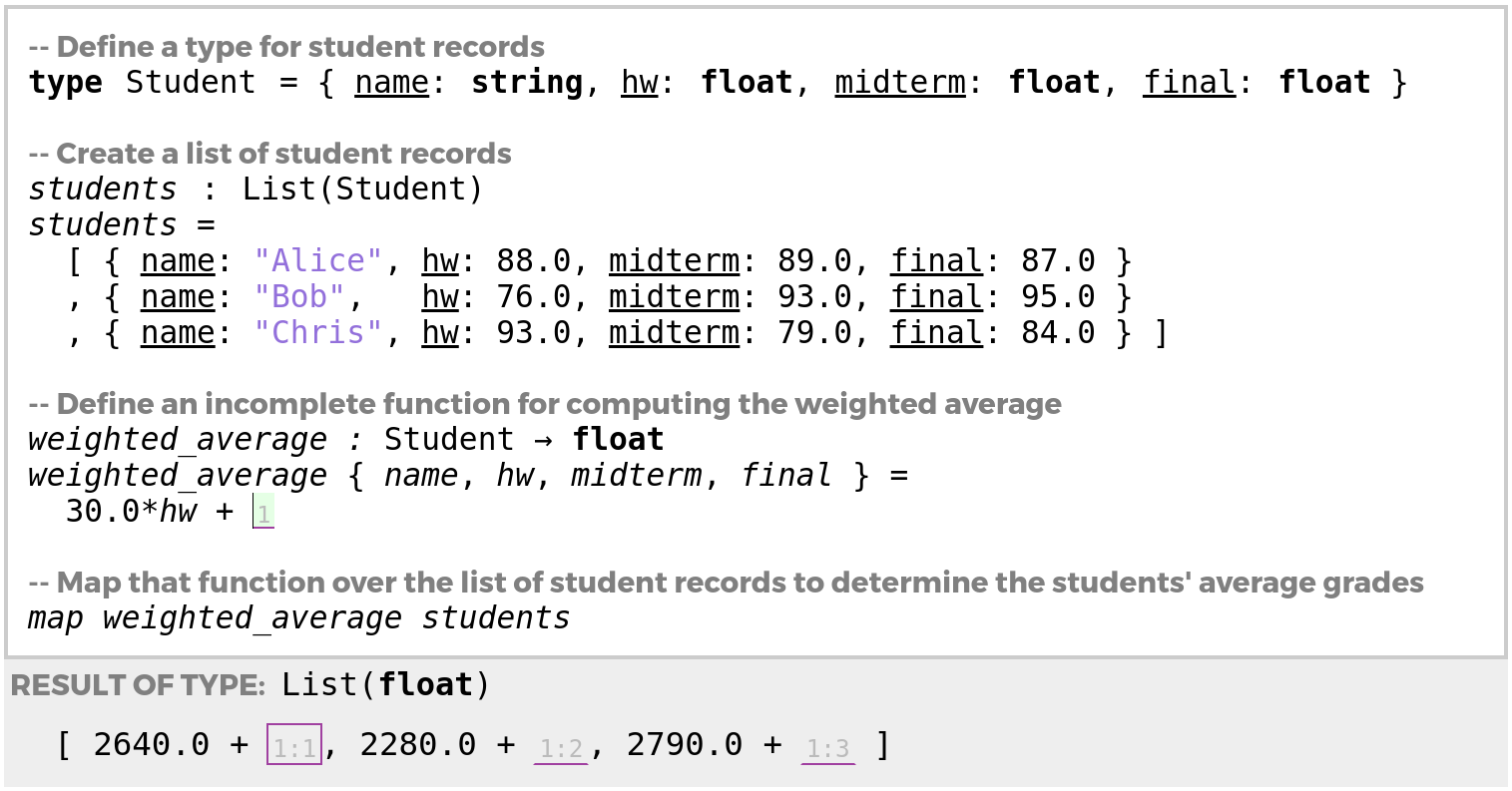
Consider the perspective of a teacher in the midst of developing a Hazel notebook to compute final student grades at the end of a course. Fig. 1(a) depicts the cell containing the incomplete program that the teacher has written so far (we omit irrelevant parts of the UI).

At the top of this program, the teacher defines a record type, Student, for recording a student’s course data—here, the student’s name, of type string, and, for simplicity, three grades, each of type float. Next, the teacher constructs a list of student records, binding it to the variable students. For simplicity, we include only three example students. At the bottom of the program, the teacher maps a function weighted_average over this student data (map is the standard map function over lists, not shown), intending to compute a final weighted average for each student. However, the program is incomplete because the teacher has not yet completed the body of the weighted_average function. This pattern is quite common: programmers often consume a function before implementing it.

Thus far in the body of weighted_average, the teacher has decomposed the function argument into variables by record destructuring, then multiplied the homework grade, hw, by 30.0 and finally inserted the + operator. In a conventional “batch” programming system, writing 30.0*hw + by itself would simply cause parsing to fail and there would be no static or dynamic feedback. In response, the programmer might temporarily raise an exception. This would cause typechecking to succeed. However, evaluation would proceed only as far as the first map iteration, which would call into weighted_average and then fail when the exception is raised.222In a lazy language, like Haskell, the result would be much the same because the environment forces the result for printing. Hazel instead inserts an empty hole at the cursor, as indicated by the vertical bar and the green background. Each hole has a unique name (generated automatically in Hazel), here simply 1.

When running the program, Hazel does not take an “exceptional” approach to holes. Instead, evaluation continues past the hole, treating it as an opaque expression of the appropriate type. The result, shown at the bottom of Fig. 1(a), is a list of length $3$, confirming that map does indeed behave as expected in this regard despite the teacher having provided an incomplete argument. Furthermore, each element of the resulting list has been evaluated as far as possible, i.e. the arithmetic expression 30.0*hw has been evaluated for each corresponding value of hw. Evaluation cannot proceed any further because holes appear as addends. We say that each of these addition expressions is an indeterminate sub-expression, and the result as a whole is therefore also indeterminate, because it is not yet a value, nor can it take a step due to holes in elimination positions.

At this point, the teacher might take notice of the magnitude of the numbers being computed, e.g. 2640.0 and 2280.0, and realize immediately that a mistake has been made: the teacher wants to compute a weighted average between 0.0 and 100.0, and so the correct constant is 0.30, not 30.0.

Although these observations might save only a small amount of time in this case, it demonstrates the broader motivations of live programming: continuous feedback about the dynamic behavior of the program can help confirm the mental model that the programmer has developed (in this case, regarding the behavior of map), and also help quickly dispel misconceptions about the actual behavior of the program (in this case, the magnitude of the arithmetic expressions being computed).

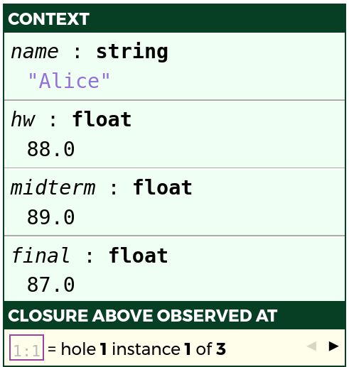
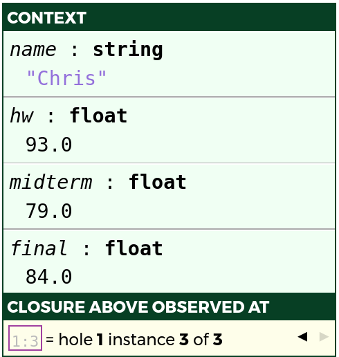
Going further, Hazel helps programmers reason about the dynamic behavior of expressions bound to variables in scope at a hole via the live context inspector, normally displayed as a sidebar but shown disembodied in three states in Fig. 1(b). In all three states, the live context inspector displays the names and types of the variables that are in scope. New to our approach are the values associated with bindings, which come from the environment associated with the selected hole instance in the result. We call a hole instance paired with an environment a hole closure, by analogy to function closures (and also due to the logical connection detailed in Sec. 3). In this case, there are three instances of hole 1 in the result, numbered sequentially 1:1, 1:2 and 1:3, arising from the three calls to weighted_averages by map. The programmer can directly select different closures by clicking on a hole instance in the result (the first instance, 1:1, is selected by default, as indicated by the purple outline in Fig. 1(a)), or cycle through all of the closures for the hole at the cursor by clicking the arrows at the bottom of the context inspector, e.g. $\blacktriangleright$, or using the corresponding keyboard shortcuts.

2.2. Example 2: Recursive Functions

Refer to caption
(a) The result of evaluation is a hole closure.
Refer to caption
(b) The type inspector provides static feedback about the term at the cursor. Currently, the hole should be filled by a list expression. Holes have the hole (i.e. unknown) type, which is universally consistent (see Sec. 3 and (Omar et al., 2017a)).
Refer to caption

$\xrightarrow[\text{click}]{}$ Refer to caption  $\xrightarrow[\text{click}]{}$ Refer to caption

(c) The programmer can explore the recursive structure of the computation by clicking on hole instances.
Figure 2. Example 2: Incomplete Quicksort

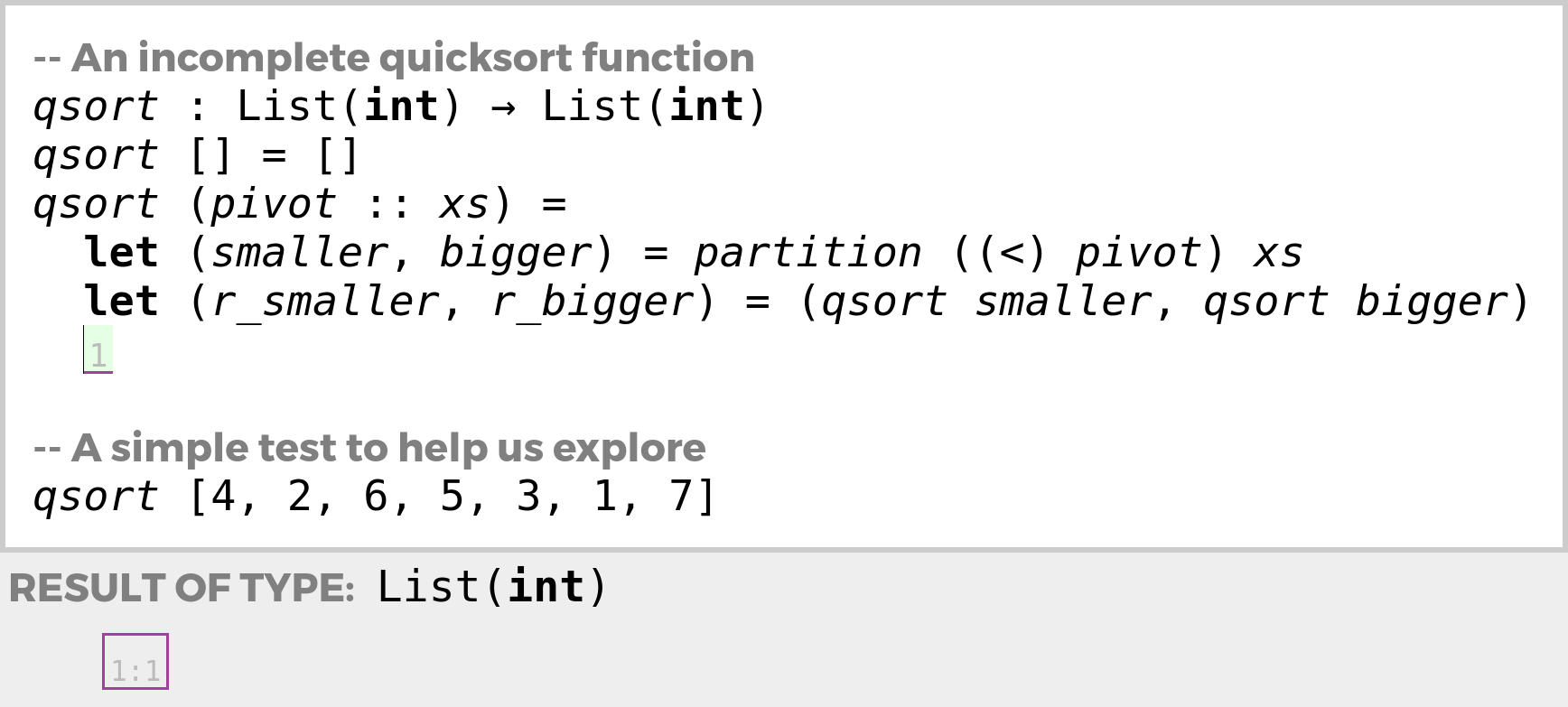
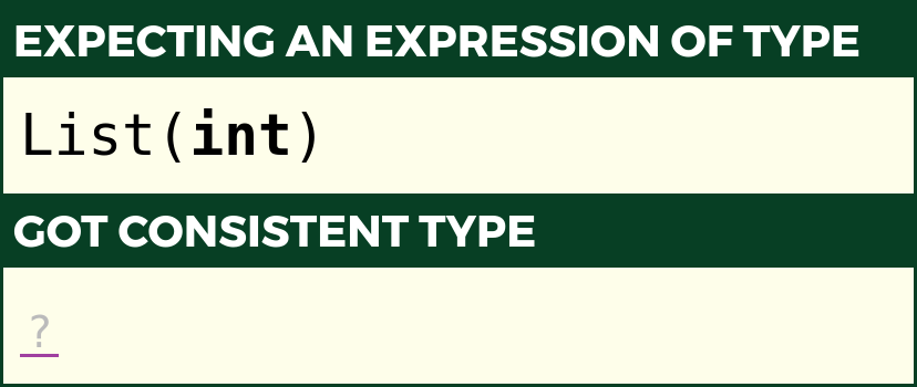
Let us now consider a second more sophisticated example: an incomplete implementation of the recursive quicksort function, shown in Fig. 2(a). So far, the programmer (perhaps a student, or a lecturer using Hazel as a presentational aid) has filled in the base case, and in the recursive case, partitioned the remainder of the list relative to the head, and made the two recursive calls. A hole appears in return position as the programmer contemplates how to fill the hole with an appropriate expression of list type, as indicated by the type inspector in Fig. 2(b).

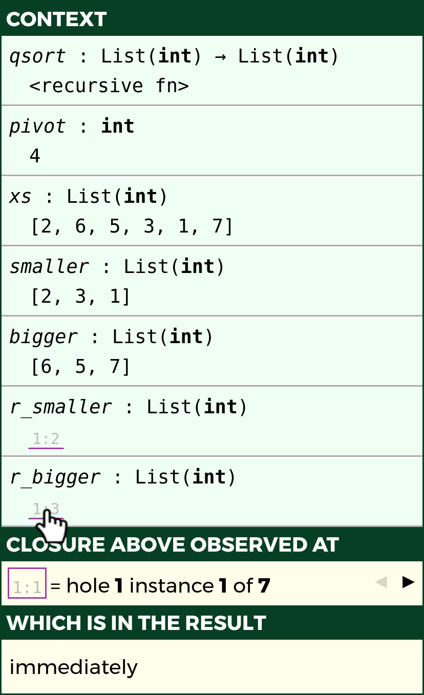
At the bottom of the cell in Fig. 2(a), the programmer has applied qsort to an example list. However, the indeterminate result of this function application is simply an instance of hole 1, which serves only to confirm that evaluation went through the recursive case of qsort. More interesting is the live context inspector, shown in three states in Fig. 2(c), which provides feedback about the values of the variables in scope at hole 1 from the the various instances of hole 1 that appear in the result, either immediately or within an outer closure. For example, in its initial state (Fig. 2(c), left) it shows the closure at the instance of hole 1 that appears immediately in the result due to the outermost application of qsort. From this, the programmer can confirm (or the lecturer can visually point out) that the lists smaller and bigger computed by the call to partition are appropriately named, and observe that they are not yet themselves sorted.

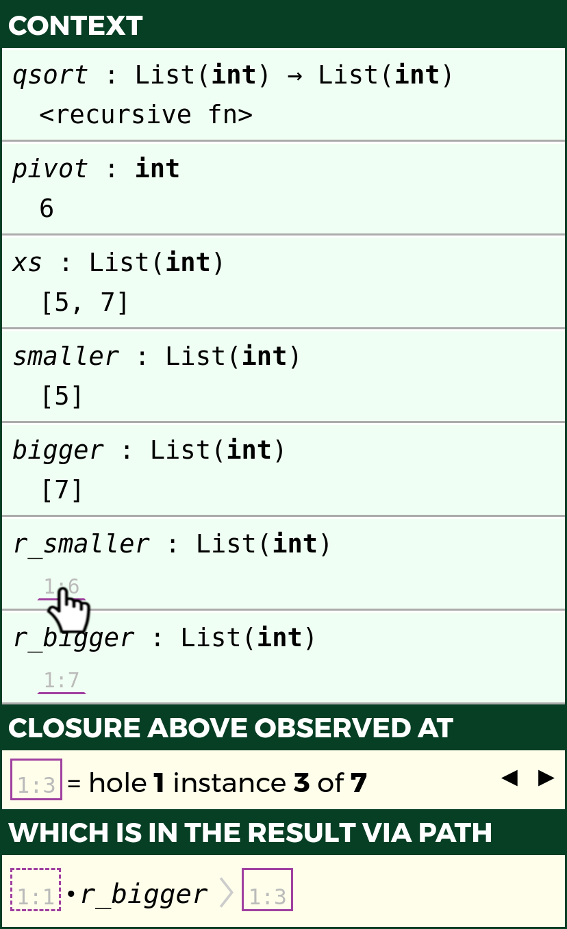
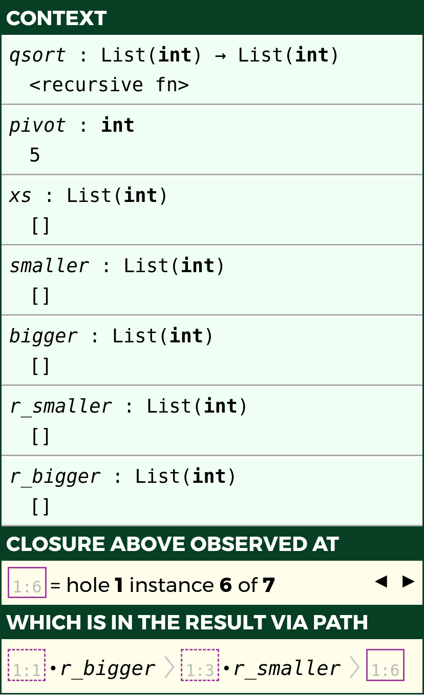
The results from the subsequent recursive calls, r_smaller and r_bigger, are again hole instances, 1:2 and 1:3. The programmer can click on either of these hole instances to reveal the associated closures from the corresponding recursive calls. For example, clicking on 1:3 reveals the hole closure from the r_bigger recursive call as shown in Fig. 2(c) (middle). From there, the programmer can click another hole closure, e.g. 1:6 to reveal the hole closure from the subsequent r_smaller recursive call as shown in Fig. 2(c) (right). Notice in each case that the path from the result to the selected hole closure is reported as shown at the bottom of the context inspector in Fig. 2(c). In exploring these paths rooted at the result, the programmer can develop concrete intuitions about the recursive structure of the computation (e.g. by following through to the base case as shown in Fig. 2(c)) even before the program is complete.

2.3. Example 3: Live Programming with Static Type Errors

Refer to caption
Figure 3. Example 3: Ill-Typed Quicksort

The previous examples were incomplete because of missing expressions. Now, we discuss programs that are incomplete, and therefore conventionally meaningless, because of type inconsistencies. Let us return to the quicksort example just described, but assume that the programmer has filled in the previous hole as shown in Fig. 3. In Sec. 4, we discuss how the programming environment could avoid restarting evaluation after such edits by using the values stored in the hole closures.

The programmer appears to be on the right track conceptually in recognizing that the pivot needs to appear between the smaller and bigger elements. However, the types do not quite work out: the @ operator here performs list concatenation, but the pivot is an integer. Most compilers and editors will report a static error message to the programmer in this case, and Hazel follows suit in the type inspector (shown inset in Fig. 3). However, our argument is that the presence of a static type error should not cause all feedback about the dynamic behavior of the program to “flicker out” or “go stale” – after all, there are perfectly meaningful parts of the program (both nearby and far away from the error) whose dynamic behavior may be of interest. Concrete results can also help the programmer understand the implications of the type error (Seidel et al., 2016).

Our approach, following the prior work of Omar et al. (2017a), is to semantically internalize the “red outline” around a type-inconsistent expression as a non-empty hole around that expression. Evaluation safely proceeds past a non-empty hole just as if it were an empty hole. The semantics also associates an environment with each instance of a non-empty hole, so we can use the live context inspector essentially as in Fig. 2(c) (not shown). Evaluation proceeds inside the hole, so that feedback about the type-inconsistent expression, which might “almost” be correct, is available. In this case, the result at the bottom of Fig. 3 reveals that the programmer is on the right track: the list elements appear in the correct order. They simply have not been combined correctly.

We are treating @ as a primitive operator in this example. If it were defined as a function, then it would be possible to further reduce the example by proceeding into the function body. This is likely unhelpful for functions other than those that programmer is actively working on. Our semantics allows beta reduction when the argument is a hole, but it does not require it.

Although Hazel inserts non-empty holes automatically, the earlier work on Hazelnut allowed the programmer to explicitly insert non-empty holes. It may be that these are useful even when there is not a type inconsistency because the non-empty hole defers elimination of the enclosed expression and causes hole closure information to be tracked. For example, if we repaired the program in Fig. 3 by replacing the erroneous variable pivot with [pivot] and then inserted a non-empty hole around this expression, the result would show all of the list concatenation operations that would be performed without actually performing them, producing a result much like that in Fig. 3. This provides another way to explore the recursive structure of the qsort function.

2.4. Example 4: Type Holes and Dynamic Type Errors

In Hazel, the program can also be incomplete because holes appear in types. Omar et al. (2017a) confirmed that the literature on gradual type systems (Siek and Taha, 2006; Siek et al., 2015a) is directly relevant to the problem of reasoning with type holes, by identifying the type hole with the unknown type. Gradual type systems can run programs that are not yet sufficiently annotated with types by inserting casts where necessary. We take the same well-studied approach in Hazel. As such, let us consider only a small synthetic example to demonstrate what is unique to our approach.

Fig. 4 defines a simple function, f, of two arguments. The type annotation on the first line leaves the type of those arguments unknown. As such, the Hazel type system, following the gradual typing approach, allows the body of the function to use those two arguments at any type (that is, the hole type is universally consistent). Here, the first argument, simple, is used at one type, bool, and the second argument, x, is used at two different types in the two branches (perhaps because the programmer made a mistake), int and string ( ^ is string concatenation). Although Hazel supports only local type inference as of this writing, a system that uses ML-style type reconstruction to fill type holes statically, like GHC Haskell, would only be able to fill the first hole. Leaving the second hole unfilled is a parsimonious alternative to arbitrarily or heuristically choosing one of the possibilities and marking the other uses of x as ill-typed (see (Chen and Erwig, 2018)).

Refer to caption
Figure 4. Example 4: Type Holes and Dynamic Type Errors

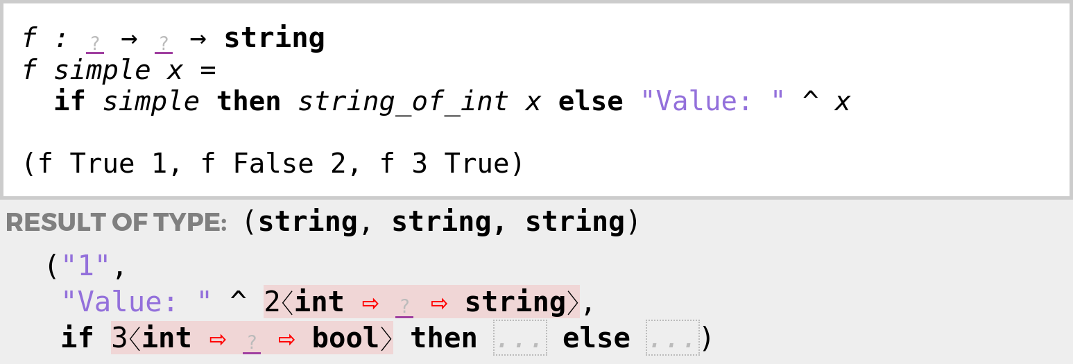
At the bottom of the cell in Fig. 4, we have three example applications of f, tupled together for concision. All three are statically well-typed, again because the hole type is universally consistent. The result at the bottom of Fig. 4 demonstrates that the first application of f is dynamically unproblematic. This allows the programmer to confirm that the first branch operates as intended without the need to address the typing problems in the other branch (Bayne et al., 2011).

The second application of f, in contrast, causes a dynamic type error because the second argument, 2, is an int but evaluation takes the branch where it is used as a string. Rather than aborting evaluation when this occurs, as in existing gradual type systems, the problematic term becomes a failed cast term, shown shaded in red, which can be read “2 is an int that was used through a variable of hole type (?) as a string”. A failed cast acts much like a non-empty hole as a membrane around a problematic term. The surrounding concatenation operation becomes indeterminate, but evaluation can continue on to the third application of f, which is also problematic, this time because the first argument is not a bool (perhaps because the programmer had an incorrect understanding of the argument order). Again, this causes a failed cast to appear, this time in guard position. Like a hole in guard position, evaluation cannot determine which branch to take so the whole conditional becomes indeterminate. The pretty printer hides the two branches behind ellipses for concision.

3. Hazelnut Live

$\begin{array}[]{rllllll}\mathsf{HTyp}&\tau&::=&b\leavevmode\nobreak\ |\leavevmode\nobreak\ \tau\rightarrow\tau\leavevmode\nobreak\ |\leavevmode\nobreak\ {\color[rgb]{.5,0,.5}\definecolor[named]{pgfstrokecolor}{rgb}{.5,0,.5}\llparenthesis}{\color[rgb]{.5,0,.5}\definecolor[named]{pgfstrokecolor}{rgb}{.5,0,.5}\rrparenthesis}\\ \mathsf{HExp}&e&::=&c\leavevmode\nobreak\ |\leavevmode\nobreak\ x\leavevmode\nobreak\ |\leavevmode\nobreak\ \lambda x{:}\tau.e\leavevmode\nobreak\ |\leavevmode\nobreak\ {\lambda x.e}\leavevmode\nobreak\ |\leavevmode\nobreak\ e(e)\leavevmode\nobreak\ |\leavevmode\nobreak\ {\color[rgb]{.5,0,.5}\definecolor[named]{pgfstrokecolor}{rgb}{.5,0,.5}\llparenthesis}{\color[rgb]{.5,0,.5}\definecolor[named]{pgfstrokecolor}{rgb}{.5,0,.5}\rrparenthesis}^{u}\leavevmode\nobreak\ |\leavevmode\nobreak\ {\color[rgb]{.5,0,.5}\definecolor[named]{pgfstrokecolor}{rgb}{.5,0,.5}\llparenthesis}e{\color[rgb]{.5,0,.5}\definecolor[named]{pgfstrokecolor}{rgb}{.5,0,.5}\rrparenthesis}^{u}\leavevmode\nobreak\ |\leavevmode\nobreak\ e:\tau\\ \mathsf{IHExp}&d&::=&c\leavevmode\nobreak\ |\leavevmode\nobreak\ x\leavevmode\nobreak\ |\leavevmode\nobreak\ {\lambda x{:}\tau.d}\leavevmode\nobreak\ |\leavevmode\nobreak\ d(d)\leavevmode\nobreak\ |\leavevmode\nobreak\ \leftidx{}{{\color[rgb]{.5,0,.5}\definecolor[named]{pgfstrokecolor}{rgb}{.5,0,.5}\llparenthesis}{\color[rgb]{.5,0,.5}\definecolor[named]{pgfstrokecolor}{rgb}{.5,0,.5}\rrparenthesis}}{{}^{u}_{\sigma}}\leavevmode\nobreak\ |\leavevmode\nobreak\ \leftidx{}{{\color[rgb]{.5,0,.5}\definecolor[named]{pgfstrokecolor}{rgb}{.5,0,.5}\llparenthesis}d{\color[rgb]{.5,0,.5}\definecolor[named]{pgfstrokecolor}{rgb}{.5,0,.5}\rrparenthesis}}{{}^{u}_{\sigma}}\leavevmode\nobreak\ |\leavevmode\nobreak\ d\langle{\tau}\Rightarrow{\tau}\rangle\leavevmode\nobreak\ |\leavevmode\nobreak\ d\langle{\tau}\Rightarrow{{\color[rgb]{.5,0,.5}\definecolor[named]{pgfstrokecolor}{rgb}{.5,0,.5}\llparenthesis}{\color[rgb]{.5,0,.5}\definecolor[named]{pgfstrokecolor}{rgb}{.5,0,.5}\rrparenthesis}}\not\Rightarrow{\tau}\rangle\\ \end{array}$

$$d\langle{\tau_{1}}\Rightarrow{\tau_{2}}\Rightarrow{\tau_{3}}\rangle\overset{\textrm{def}}{=}d\langle{\tau_{1}}\Rightarrow{\tau_{2}}\rangle\langle{\tau_{2}}\Rightarrow{\tau_{3}}\rangle$$
Figure 5. Syntax of types, $\tau$, external expressions, $e$, and internal expressions, $d$. We write $x$ to range over variables, $u$ over hole names, and $\sigma$ over finite substitutions (i.e., environments) which map variables to internal expressions, written $d_{1}/x_{1},\leavevmode\nobreak\ \cdots,d_{n}/x_{n}$ for $n\geq 0$.

We will now make the intuitions developed in the previous section formally precise by specifying a core calculus, which we call Hazelnut Live, and characterizing its metatheory.

Overview.

The syntax of the core calculus given in Fig. 5 consists of types and expressions with holes. We distinguish between external expressions, $e$, and internal expressions, $d$. External expressions correspond to programs as entered by the programmer (see Sec. 1 for discussion of implicit, manual, semi-automated and fully automated hole entry methods). Each well-typed external expression (see Sec. 3.1 below) elaborates to a well-typed internal expression (see Sec. 3.2) before it is evaluated (see Sec. 3.3). We take this approach, notably also taken in the “redefinition” of Standard ML by Harper and Stone (2000), because (1) the external language supports type inference and explicit type ascriptions, $e:\tau$, but it is formally simpler to eliminate ascriptions and specify a type assignment system when defining the dynamic semantics; and (2) we need additional syntactic machinery during evaluation for tracking hole closures and dynamic type casts. This machinery is inserted by elaboration, rather than entered explicitly by the programmer. In this regard, the internal language is analogous to the cast calculus in the gradually typed lambda calculus (Siek et al., 2015a; Siek and Taha, 2006), though as we will see the Hazelnut Live internal language goes beyond the cast calculus in several respects. We have mechanized these formal developments using the Agda proof assistant (Norell, 2007, 2009) (see Sec. 3.4). Rule names in this section, e.g. SVar, correspond to variables from the mechanization. The Hazel implementation substantially follows the formal specification of Hazelnut (for the editor) and Hazelnut Live (for the evaluator). We can formally state a continuity invariant for a putative combined calculus (see Sec. 3.5).

3.1. Static Semantics of the External Language

$\Gamma\vdash e\Rightarrow\tau$ $e$ synthesizes type $\tau$

SConst   $\displaystyle\displaystyle{\hbox{}\over\hbox{\hskip 21.04561pt\vbox{\vbox{}\hbox{\hskip-21.0456pt\hbox{\hbox{$\displaystyle\displaystyle\Gamma\vdash c\Rightarrow b$}}}}}}$        SVar   $\displaystyle\displaystyle{\hbox{\hskip 18.44608pt\vbox{\hbox{\hskip-18.44606pt\hbox{\hbox{$\displaystyle\displaystyle x:\tau\in\Gamma$}}}\vbox{}}}\over\hbox{\hskip 21.7794pt\vbox{\vbox{}\hbox{\hskip-21.77939pt\hbox{\hbox{$\displaystyle\displaystyle\Gamma\vdash x\Rightarrow\tau$}}}}}}$        SLam   $\displaystyle\displaystyle{\hbox{\hskip 33.5377pt\vbox{\hbox{\hskip-33.53769pt\hbox{\hbox{$\displaystyle\displaystyle\Gamma,x:\tau_{1}\vdash e\Rightarrow\tau_{2}$}}}\vbox{}}}\over\hbox{\hskip 43.09572pt\vbox{\vbox{}\hbox{\hskip-43.0957pt\hbox{\hbox{$\displaystyle\displaystyle\Gamma\vdash\lambda x{:}\tau_{1}.e\Rightarrow\tau_{1}\rightarrow\tau_{2}$}}}}}}$        SAp   $\displaystyle\displaystyle{\hbox{\hskip 72.52667pt\vbox{\hbox{\hskip-72.52666pt\hbox{\hbox{$\displaystyle\displaystyle\Gamma\vdash e_{1}\Rightarrow\tau_{1}$}\hskip 20.00003pt\hbox{\hbox{$\displaystyle\displaystyle\tau_{1}\blacktriangleright_{\rightarrow}\tau_{2}\rightarrow\tau$}\hskip 20.00003pt\hbox{\hskip-22.66104pt\hbox{\hbox{$\displaystyle\displaystyle\Gamma\vdash e_{2}\Leftarrow\tau_{2}$}}}}}}\vbox{\hbox{\hskip-22.66104pt\hbox{\hbox{$\displaystyle\displaystyle\Gamma\vdash e_{2}\Leftarrow\tau_{2}$}}}\vbox{}}}}\over\hbox{\hskip 30.26694pt\vbox{\vbox{}\hbox{\hskip-30.26692pt\hbox{\hbox{$\displaystyle\displaystyle\Gamma\vdash e_{1}(e_{2})\Rightarrow\tau$}}}}}}$        SEHole   $\displaystyle\displaystyle{\hbox{}\over\hbox{\hskip 29.17232pt\vbox{\vbox{}\hbox{\hskip-29.1723pt\hbox{\hbox{$\displaystyle\displaystyle\Gamma\vdash{\color[rgb]{.5,0,.5}\definecolor[named]{pgfstrokecolor}{rgb}{.5,0,.5}\llparenthesis}{\color[rgb]{.5,0,.5}\definecolor[named]{pgfstrokecolor}{rgb}{.5,0,.5}\rrparenthesis}^{u}\Rightarrow{\color[rgb]{.5,0,.5}\definecolor[named]{pgfstrokecolor}{rgb}{.5,0,.5}\llparenthesis}{\color[rgb]{.5,0,.5}\definecolor[named]{pgfstrokecolor}{rgb}{.5,0,.5}\rrparenthesis}$}}}}}}$        SNEHole   $\displaystyle\displaystyle{\hbox{\hskip 21.2499pt\vbox{\hbox{\hskip-21.2499pt\hbox{\hbox{$\displaystyle\displaystyle\Gamma\vdash e\Rightarrow\tau$}}}\vbox{}}}\over\hbox{\hskip 31.50044pt\vbox{\vbox{}\hbox{\hskip-31.50044pt\hbox{\hbox{$\displaystyle\displaystyle\Gamma\vdash{\color[rgb]{.5,0,.5}\definecolor[named]{pgfstrokecolor}{rgb}{.5,0,.5}\llparenthesis}e{\color[rgb]{.5,0,.5}\definecolor[named]{pgfstrokecolor}{rgb}{.5,0,.5}\rrparenthesis}^{u}\Rightarrow{\color[rgb]{.5,0,.5}\definecolor[named]{pgfstrokecolor}{rgb}{.5,0,.5}\llparenthesis}{\color[rgb]{.5,0,.5}\definecolor[named]{pgfstrokecolor}{rgb}{.5,0,.5}\rrparenthesis}$}}}}}}$        SAsc   $\displaystyle\displaystyle{\hbox{\hskip 21.2499pt\vbox{\hbox{\hskip-21.2499pt\hbox{\hbox{$\displaystyle\displaystyle\Gamma\vdash e\Leftarrow\tau$}}}\vbox{}}}\over\hbox{\hskip 27.60226pt\vbox{\vbox{}\hbox{\hskip-27.60226pt\hbox{\hbox{$\displaystyle\displaystyle\Gamma\vdash e:\tau\Rightarrow\tau$}}}}}}$

$\Gamma\vdash e\Leftarrow\tau$ $e$ analyzes against type $\tau$

ALam   $\displaystyle\displaystyle{\hbox{\hskip 63.46164pt\vbox{\hbox{\hskip-63.46164pt\hbox{\hbox{$\displaystyle\displaystyle\tau\blacktriangleright_{\rightarrow}\tau_{1}\rightarrow\tau_{2}$}\hskip 20.00003pt\hbox{\hbox{$\displaystyle\displaystyle\Gamma,x:\tau_{1}\vdash e\Leftarrow\tau_{2}$}}}}\vbox{}}}\over\hbox{\hskip 29.24641pt\vbox{\vbox{}\hbox{\hskip-29.24641pt\hbox{\hbox{$\displaystyle\displaystyle\Gamma\vdash\lambda x.e\Leftarrow\tau$}}}}}}$        ASubsume   $\displaystyle\displaystyle{\hbox{\hskip 43.05806pt\vbox{\hbox{\hskip-43.05804pt\hbox{\hbox{$\displaystyle\displaystyle\Gamma\vdash e\Rightarrow\tau$}\hskip 20.00003pt\hbox{\hbox{$\displaystyle\displaystyle\tau\sim\tau^{\prime}$}}}}\vbox{}}}\over\hbox{\hskip 22.0199pt\vbox{\vbox{}\hbox{\hskip-22.01988pt\hbox{\hbox{$\displaystyle\displaystyle\Gamma\vdash e\Leftarrow\tau^{\prime}$}}}}}}$
Figure 6. Bidirectional Typing of External Expressions

We start with the type system of the Hazelnut Live external language, which closely follows the Hazelnut type system (Omar et al., 2017a); we summarize the minor differences as they come up.

Fig. 6 defines the type system in the bidirectional style with two mutually defined judgements (Pierce and Turner, 2000; Christiansen, 2013; Dunfield and Krishnaswami, 2013; Chlipala et al., 2005). The type synthesis judgement $\Gamma\vdash e\Rightarrow\tau$ synthesizes a type $\tau$ for external expression $e$ under typing context $\Gamma$, which tracks typing assumptions of the form $x:\tau$ in the usual manner (Harper, 2016; Pierce, 2002). The type analysis judgement $\Gamma\vdash e\Leftarrow\tau$ checks expression $e$ against a given type $\tau$. Algorithmically, analysis accepts a type as input, and synthesis gives a type as output. We start with synthesis for the programmer’s top level external expression.

The primary benefit of specifying the Hazelnut Live external language bidirectionally is that the programmer need not annotate each hole with a type. An empty hole is written simply ${\color[rgb]{.5,0,.5}\definecolor[named]{pgfstrokecolor}{rgb}{.5,0,.5}\llparenthesis}{\color[rgb]{.5,0,.5}\definecolor[named]{pgfstrokecolor}{rgb}{.5,0,.5}\rrparenthesis}^{u}$, where $u$ is the hole name, which we tacitly assume is unique (holes in Hazelnut were not named). Rule SEHole specifies that an empty hole synthesizes hole type, written ${\color[rgb]{.5,0,.5}\definecolor[named]{pgfstrokecolor}{rgb}{.5,0,.5}\llparenthesis}{\color[rgb]{.5,0,.5}\definecolor[named]{pgfstrokecolor}{rgb}{.5,0,.5}\rrparenthesis}$. If an empty hole appears where an expression of some other type is expected, e.g. under an explicit ascription (governed by Rule SAsc) or in the argument position of a function application (governed by Rule SAp, discussed below), we apply the subsumption rule, Rule ASubsume, which specifies that if an expression $e$ synthesizes type $\tau$, then it may be checked against any consistent type, $\tau^{\prime}$.

$\tau_{1}\sim\tau_{2}$ $\tau_{1}$ is consistent with $\tau_{2}$

TCHole1   $\displaystyle\displaystyle{\hbox{}\over\hbox{\hskip 14.96353pt\vbox{\vbox{}\hbox{\hskip-14.96352pt\hbox{\hbox{$\displaystyle\displaystyle{\color[rgb]{.5,0,.5}\definecolor[named]{pgfstrokecolor}{rgb}{.5,0,.5}\llparenthesis}{\color[rgb]{.5,0,.5}\definecolor[named]{pgfstrokecolor}{rgb}{.5,0,.5}\rrparenthesis}\sim\tau$}}}}}}$        TCHole2   $\displaystyle\displaystyle{\hbox{}\over\hbox{\hskip 14.96353pt\vbox{\vbox{}\hbox{\hskip-14.96352pt\hbox{\hbox{$\displaystyle\displaystyle\tau\sim{\color[rgb]{.5,0,.5}\definecolor[named]{pgfstrokecolor}{rgb}{.5,0,.5}\llparenthesis}{\color[rgb]{.5,0,.5}\definecolor[named]{pgfstrokecolor}{rgb}{.5,0,.5}\rrparenthesis}$}}}}}}$        TCRefl   $\displaystyle\displaystyle{\hbox{}\over\hbox{\hskip 11.03815pt\vbox{\vbox{}\hbox{\hskip-11.03815pt\hbox{\hbox{$\displaystyle\displaystyle\tau\sim\tau$}}}}}}$        TCArr   $\displaystyle\displaystyle{\hbox{\hskip 34.8986pt\vbox{\hbox{\hskip-34.8986pt\hbox{\hbox{$\displaystyle\displaystyle\tau_{1}\sim\tau_{1}^{\prime}$}\hskip 20.00003pt\hbox{\hbox{$\displaystyle\displaystyle\tau_{2}\sim\tau_{2}^{\prime}$}}}}\vbox{}}}\over\hbox{\hskip 27.39856pt\vbox{\vbox{}\hbox{\hskip-27.39856pt\hbox{\hbox{$\displaystyle\displaystyle\tau_{1}\rightarrow\tau_{2}\sim\tau_{1}^{\prime}\rightarrow\tau_{2}^{\prime}$}}}}}}$

$\tau\blacktriangleright_{\rightarrow}\tau_{1}\rightarrow\tau_{2}$ $\tau$ has matched arrow type $\tau_{1}\rightarrow\tau_{2}$

MAHole     $\displaystyle\displaystyle{\hbox{}\over\hbox{\hskip 30.28891pt\vbox{\vbox{}\hbox{\hskip-30.28891pt\hbox{\hbox{$\displaystyle\displaystyle{\color[rgb]{.5,0,.5}\definecolor[named]{pgfstrokecolor}{rgb}{.5,0,.5}\llparenthesis}{\color[rgb]{.5,0,.5}\definecolor[named]{pgfstrokecolor}{rgb}{.5,0,.5}\rrparenthesis}\blacktriangleright_{\rightarrow}{\color[rgb]{.5,0,.5}\definecolor[named]{pgfstrokecolor}{rgb}{.5,0,.5}\llparenthesis}{\color[rgb]{.5,0,.5}\definecolor[named]{pgfstrokecolor}{rgb}{.5,0,.5}\rrparenthesis}\rightarrow{\color[rgb]{.5,0,.5}\definecolor[named]{pgfstrokecolor}{rgb}{.5,0,.5}\llparenthesis}{\color[rgb]{.5,0,.5}\definecolor[named]{pgfstrokecolor}{rgb}{.5,0,.5}\rrparenthesis}$}}}}}}$        MAArr   $\displaystyle\displaystyle{\hbox{}\over\hbox{\hskip 27.40971pt\vbox{\vbox{}\hbox{\hskip-27.4097pt\hbox{\hbox{$\displaystyle\displaystyle\tau_{1}\rightarrow\tau_{2}\blacktriangleright_{\rightarrow}\tau_{1}\rightarrow\tau_{2}$}}}}}}$
Figure 7. Type Consistency and Matching

Fig. 7 specifies the type consistency relation, written $\tau\sim\tau^{\prime}$, which specifies that two types are consistent if they differ only up to type holes in corresponding positions. The hole type is consistent with every type, and so, by the subsumption rule, expression holes may appear where an expression of any type is expected. The type consistency relation here coincides with the type consistency relation from gradual type theory by identifying the hole type with the unknown type (Siek and Taha, 2006). Type consistency is reflexive and symmetric, but it is not transitive. This stands in contrast to subtyping, which is anti-symmetric and transitive; subtyping may be integrated into a gradual type system following Siek and Taha (2007).

Non-empty expression holes, written ${\color[rgb]{.5,0,.5}\definecolor[named]{pgfstrokecolor}{rgb}{.5,0,.5}\llparenthesis}e{\color[rgb]{.5,0,.5}\definecolor[named]{pgfstrokecolor}{rgb}{.5,0,.5}\rrparenthesis}^{u}$, behave similarly to empty holes. Rule SNEHole specifies that a non-empty expression hole also synthesizes hole type as long as the expression inside the hole, $e$, synthesizes some (arbitrary) type. Non-empty expression holes therefore internalize the “red underline/outline” that many editors display around type inconsistencies in a program.

For the familiar forms of the lambda calculus, the rules again follow prior work. For simplicity, the core calculus includes only a single base type $b$ with a single constant $c$, governed by Rule SConst (i.e. $b$ is the unit type). By contrast, Omar et al. (2017a) instead defined a number type with a single operation. That paper also defined sum types as an extension to the core calculus. We follow suit on both counts in Appendix B.

Rule SVar synthesizes the corresponding type from $\Gamma$. For the sake of exposition, Hazelnut Live includes “half-annotated” lambdas, $\lambda x{:}\tau.e$, in addition to the unannotated lambdas, $\lambda x.e$, from Hazelnut. Half-annotated lambdas may appear in synthetic position according to Rule SLam, which is standard (Chlipala et al., 2005). Unannotated lambdas may only appear where the expected type is known to be either an arrow type or the hole type, which is treated as if it were ${\color[rgb]{.5,0,.5}\definecolor[named]{pgfstrokecolor}{rgb}{.5,0,.5}\llparenthesis}{\color[rgb]{.5,0,.5}\definecolor[named]{pgfstrokecolor}{rgb}{.5,0,.5}\rrparenthesis}\rightarrow{\color[rgb]{.5,0,.5}\definecolor[named]{pgfstrokecolor}{rgb}{.5,0,.5}\llparenthesis}{\color[rgb]{.5,0,.5}\definecolor[named]{pgfstrokecolor}{rgb}{.5,0,.5}\rrparenthesis}$.333A system supporting ML-style type reconstruction (Damas and Milner, 1982) might also include a synthetic rule for unannotated lambdas, e.g. as outlined by Dunfield and Krishnaswami (2013), but we stick to this simpler “Scala-style” local type inference scheme in this paper (Pierce and Turner, 2000; Odersky et al., 2001). To avoid the need for separate rules for these two cases, Rule ALam uses the matching relation $\tau\blacktriangleright_{\rightarrow}\tau_{1}\rightarrow\tau_{2}$ defined in Fig. 7, which produces the matched arrow type ${\color[rgb]{.5,0,.5}\definecolor[named]{pgfstrokecolor}{rgb}{.5,0,.5}\llparenthesis}{\color[rgb]{.5,0,.5}\definecolor[named]{pgfstrokecolor}{rgb}{.5,0,.5}\rrparenthesis}\rightarrow{\color[rgb]{.5,0,.5}\definecolor[named]{pgfstrokecolor}{rgb}{.5,0,.5}\llparenthesis}{\color[rgb]{.5,0,.5}\definecolor[named]{pgfstrokecolor}{rgb}{.5,0,.5}\rrparenthesis}$ given the hole type, and operates as the identity on arrow types (Siek et al., 2015a; Garcia and Cimini, 2015). The rule governing function application, Rule SAp, similarly treats an expression of hole type in function position as if it were of type ${\color[rgb]{.5,0,.5}\definecolor[named]{pgfstrokecolor}{rgb}{.5,0,.5}\llparenthesis}{\color[rgb]{.5,0,.5}\definecolor[named]{pgfstrokecolor}{rgb}{.5,0,.5}\rrparenthesis}\rightarrow{\color[rgb]{.5,0,.5}\definecolor[named]{pgfstrokecolor}{rgb}{.5,0,.5}\llparenthesis}{\color[rgb]{.5,0,.5}\definecolor[named]{pgfstrokecolor}{rgb}{.5,0,.5}\rrparenthesis}$ using the same matching relation.

We do not formally need an explicit fixpoint operator because this calculus supports general recursion due to type holes, e.g. we can express the Y combinator as $(\lambda x{:}{\color[rgb]{.5,0,.5}\definecolor[named]{pgfstrokecolor}{rgb}{.5,0,.5}\llparenthesis}{\color[rgb]{.5,0,.5}\definecolor[named]{pgfstrokecolor}{rgb}{.5,0,.5}\rrparenthesis}.x(x))(\lambda x{:}{\color[rgb]{.5,0,.5}\definecolor[named]{pgfstrokecolor}{rgb}{.5,0,.5}\llparenthesis}{\color[rgb]{.5,0,.5}\definecolor[named]{pgfstrokecolor}{rgb}{.5,0,.5}\rrparenthesis}.x(x))$. More generally, the untyped lambda calculus can be embedded as described by Siek and Taha (2006).

3.2. Elaboration

$\Gamma\vdash e\Rightarrow\tau\leadsto d\dashv\Delta$ $e$ synthesizes type $\tau$ and elaborates to $d$

ESConst   $\displaystyle\displaystyle{\hbox{}\over\hbox{\hskip 39.32037pt\vbox{\vbox{}\hbox{\hskip-39.32037pt\hbox{\hbox{$\displaystyle\displaystyle\Gamma\vdash c\Rightarrow b\leadsto c\dashv\emptyset$}}}}}}$        ESVar   $\displaystyle\displaystyle{\hbox{\hskip 18.44608pt\vbox{\hbox{\hskip-18.44606pt\hbox{\hbox{$\displaystyle\displaystyle x:\tau\in\Gamma$}}}\vbox{}}}\over\hbox{\hskip 40.74803pt\vbox{\vbox{}\hbox{\hskip-40.74802pt\hbox{\hbox{$\displaystyle\displaystyle\Gamma\vdash x\Rightarrow\tau\leadsto x\dashv\emptyset$}}}}}}$        ESLam   $\displaystyle\displaystyle{\hbox{\hskip 52.52895pt\vbox{\hbox{\hskip-52.52893pt\hbox{\hbox{$\displaystyle\displaystyle\Gamma,x:\tau_{1}\vdash e\Rightarrow\tau_{2}\leadsto d\dashv\Delta$}}}\vbox{}}}\over\hbox{\hskip 75.05814pt\vbox{\vbox{}\hbox{\hskip-75.05814pt\hbox{\hbox{$\displaystyle\displaystyle\Gamma\vdash\lambda x{:}\tau_{1}.e\Rightarrow\tau_{1}\rightarrow\tau_{2}\leadsto\lambda x{:}\tau_{1}.d\dashv\Delta$}}}}}}$        ESAp   $\displaystyle\displaystyle{\hbox{\hskip 117.96599pt\vbox{\hbox{\hskip-117.96599pt\hbox{\hbox{$\displaystyle\displaystyle\Gamma\vdash e_{1}\Rightarrow\tau_{1}$}\hskip 20.00003pt\hbox{\hbox{$\displaystyle\displaystyle\tau_{1}\blacktriangleright_{\rightarrow}\tau_{2}\rightarrow\tau$}\hskip 20.00003pt\hbox{\hskip-116.3174pt\hbox{\hbox{$\displaystyle\displaystyle\Gamma\vdash e_{1}\Leftarrow\tau_{2}\rightarrow\tau\leadsto d_{1}:\tau_{1}^{\prime}\dashv\Delta_{1}$}\hskip 20.00003pt\hbox{\hbox{$\displaystyle\displaystyle\Gamma\vdash e_{2}\Leftarrow\tau_{2}\leadsto d_{2}:\tau_{2}^{\prime}\dashv\Delta_{2}$}}}}}}}\vbox{\hbox{\hskip-116.3174pt\hbox{\hbox{$\displaystyle\displaystyle\Gamma\vdash e_{1}\Leftarrow\tau_{2}\rightarrow\tau\leadsto d_{1}:\tau_{1}^{\prime}\dashv\Delta_{1}$}\hskip 20.00003pt\hbox{\hbox{$\displaystyle\displaystyle\Gamma\vdash e_{2}\Leftarrow\tau_{2}\leadsto d_{2}:\tau_{2}^{\prime}\dashv\Delta_{2}$}}}}\vbox{}}}}\over\hbox{\hskip 113.4339pt\vbox{\vbox{}\hbox{\hskip-113.4339pt\hbox{\hbox{$\displaystyle\displaystyle\Gamma\vdash e_{1}(e_{2})\Rightarrow\tau\leadsto(d_{1}\langle{\tau_{1}^{\prime}}\Rightarrow{\tau_{2}\rightarrow\tau}\rangle)(d_{2}\langle{\tau_{2}^{\prime}}\Rightarrow{\tau_{2}}\rangle)\dashv\Delta_{1}\cup\Delta_{2}$}}}}}}$        ESEHole   $\displaystyle\displaystyle{\hbox{}\over\hbox{\hskip 72.68605pt\vbox{\vbox{}\hbox{\hskip-72.68605pt\hbox{\hbox{$\displaystyle\displaystyle\Gamma\vdash{\color[rgb]{.5,0,.5}\definecolor[named]{pgfstrokecolor}{rgb}{.5,0,.5}\llparenthesis}{\color[rgb]{.5,0,.5}\definecolor[named]{pgfstrokecolor}{rgb}{.5,0,.5}\rrparenthesis}^{u}\Rightarrow{\color[rgb]{.5,0,.5}\definecolor[named]{pgfstrokecolor}{rgb}{.5,0,.5}\llparenthesis}{\color[rgb]{.5,0,.5}\definecolor[named]{pgfstrokecolor}{rgb}{.5,0,.5}\rrparenthesis}\leadsto\leftidx{}{{\color[rgb]{.5,0,.5}\definecolor[named]{pgfstrokecolor}{rgb}{.5,0,.5}\llparenthesis}{\color[rgb]{.5,0,.5}\definecolor[named]{pgfstrokecolor}{rgb}{.5,0,.5}\rrparenthesis}}{{}^{u}_{\mathsf{id}(\Gamma)}}\dashv u::{\color[rgb]{.5,0,.5}\definecolor[named]{pgfstrokecolor}{rgb}{.5,0,.5}\llparenthesis}{\color[rgb]{.5,0,.5}\definecolor[named]{pgfstrokecolor}{rgb}{.5,0,.5}\rrparenthesis}[\Gamma]$}}}}}}$        ESNEHole   $\displaystyle\displaystyle{\hbox{\hskip 41.62999pt\vbox{\hbox{\hskip-41.62999pt\hbox{\hbox{$\displaystyle\displaystyle\Gamma\vdash e\Rightarrow\tau\leadsto d\dashv\Delta$}}}\vbox{}}}\over\hbox{\hskip 84.00551pt\vbox{\vbox{}\hbox{\hskip-84.0055pt\hbox{\hbox{$\displaystyle\displaystyle\Gamma\vdash{\color[rgb]{.5,0,.5}\definecolor[named]{pgfstrokecolor}{rgb}{.5,0,.5}\llparenthesis}e{\color[rgb]{.5,0,.5}\definecolor[named]{pgfstrokecolor}{rgb}{.5,0,.5}\rrparenthesis}^{u}\Rightarrow{\color[rgb]{.5,0,.5}\definecolor[named]{pgfstrokecolor}{rgb}{.5,0,.5}\llparenthesis}{\color[rgb]{.5,0,.5}\definecolor[named]{pgfstrokecolor}{rgb}{.5,0,.5}\rrparenthesis}\leadsto\leftidx{}{{\color[rgb]{.5,0,.5}\definecolor[named]{pgfstrokecolor}{rgb}{.5,0,.5}\llparenthesis}d{\color[rgb]{.5,0,.5}\definecolor[named]{pgfstrokecolor}{rgb}{.5,0,.5}\rrparenthesis}}{{}^{u}_{\mathsf{id}(\Gamma)}}\dashv\Delta,u::{\color[rgb]{.5,0,.5}\definecolor[named]{pgfstrokecolor}{rgb}{.5,0,.5}\llparenthesis}{\color[rgb]{.5,0,.5}\definecolor[named]{pgfstrokecolor}{rgb}{.5,0,.5}\rrparenthesis}[\Gamma]$}}}}}}$        ESAsc   $\displaystyle\displaystyle{\hbox{\hskip 47.36351pt\vbox{\hbox{\hskip-47.3635pt\hbox{\hbox{$\displaystyle\displaystyle\Gamma\vdash e\Leftarrow\tau\leadsto d:\tau^{\prime}\dashv\Delta$}}}\vbox{}}}\over\hbox{\hskip 60.62395pt\vbox{\vbox{}\hbox{\hskip-60.62395pt\hbox{\hbox{$\displaystyle\displaystyle\Gamma\vdash e:\tau\Rightarrow\tau\leadsto d\langle{\tau^{\prime}}\Rightarrow{\tau}\rangle\dashv\Delta$}}}}}}$

$\Gamma\vdash e\Leftarrow\tau_{1}\leadsto d:\tau_{2}\dashv\Delta$ $e$ analyzes against type $\tau_{1}$ and elaborates to $d$ of consistent type $\tau_{2}$

EALam   $\displaystyle\displaystyle{\hbox{\hskip 88.1864pt\vbox{\hbox{\hskip-88.18639pt\hbox{\hbox{$\displaystyle\displaystyle\tau\blacktriangleright_{\rightarrow}\tau_{1}\rightarrow\tau_{2}$}\hskip 20.00003pt\hbox{\hbox{$\displaystyle\displaystyle\Gamma,x:\tau_{1}\vdash e\Leftarrow\tau_{2}\leadsto d:\tau^{\prime}_{2}\dashv\Delta$}}}}\vbox{}}}\over\hbox{\hskip 75.047pt\vbox{\vbox{}\hbox{\hskip-75.04698pt\hbox{\hbox{$\displaystyle\displaystyle\Gamma\vdash\lambda x.e\Leftarrow\tau\leadsto\lambda x{:}\tau_{1}.d:\tau_{1}\rightarrow\tau_{2}^{\prime}\dashv\Delta$}}}}}}$        EASubsume   $\displaystyle\displaystyle{\hbox{\hskip 87.64755pt\vbox{\hbox{\hskip-87.64754pt\hbox{\hbox{$\displaystyle\displaystyle e\neq{\color[rgb]{.5,0,.5}\definecolor[named]{pgfstrokecolor}{rgb}{.5,0,.5}\llparenthesis}{\color[rgb]{.5,0,.5}\definecolor[named]{pgfstrokecolor}{rgb}{.5,0,.5}\rrparenthesis}^{u}$}\hskip 20.00003pt\hbox{\hbox{$\displaystyle\displaystyle e\neq{\color[rgb]{.5,0,.5}\definecolor[named]{pgfstrokecolor}{rgb}{.5,0,.5}\llparenthesis}e^{\prime}{\color[rgb]{.5,0,.5}\definecolor[named]{pgfstrokecolor}{rgb}{.5,0,.5}\rrparenthesis}^{u}$}\hskip 20.00003pt\hbox{\hskip-62.81929pt\hbox{\hbox{$\displaystyle\displaystyle\Gamma\vdash e\Rightarrow\tau^{\prime}\leadsto d\dashv\Delta$}\hskip 20.00003pt\hbox{\hbox{$\displaystyle\displaystyle\tau\sim\tau^{\prime}$}}}}}}}\vbox{\hbox{\hskip-62.81929pt\hbox{\hbox{$\displaystyle\displaystyle\Gamma\vdash e\Rightarrow\tau^{\prime}\leadsto d\dashv\Delta$}\hskip 20.00003pt\hbox{\hbox{$\displaystyle\displaystyle\tau\sim\tau^{\prime}$}}}}\vbox{}}}}\over\hbox{\hskip 47.36351pt\vbox{\vbox{}\hbox{\hskip-47.3635pt\hbox{\hbox{$\displaystyle\displaystyle\Gamma\vdash e\Leftarrow\tau\leadsto d:\tau^{\prime}\dashv\Delta$}}}}}}$        EAEHole   $\displaystyle\displaystyle{\hbox{}\over\hbox{\hskip 71.18767pt\vbox{\vbox{}\hbox{\hskip-71.18767pt\hbox{\hbox{$\displaystyle\displaystyle\Gamma\vdash{\color[rgb]{.5,0,.5}\definecolor[named]{pgfstrokecolor}{rgb}{.5,0,.5}\llparenthesis}{\color[rgb]{.5,0,.5}\definecolor[named]{pgfstrokecolor}{rgb}{.5,0,.5}\rrparenthesis}^{u}\Leftarrow\tau\leadsto\leftidx{}{{\color[rgb]{.5,0,.5}\definecolor[named]{pgfstrokecolor}{rgb}{.5,0,.5}\llparenthesis}{\color[rgb]{.5,0,.5}\definecolor[named]{pgfstrokecolor}{rgb}{.5,0,.5}\rrparenthesis}}{{}^{u}_{\mathsf{id}(\Gamma)}}:\tau\dashv u::\tau[\Gamma]$}}}}}}$        EANEHole   $\displaystyle\displaystyle{\hbox{\hskip 41.01114pt\vbox{\hbox{\hskip-41.01112pt\hbox{\hbox{$\displaystyle\displaystyle\Gamma\vdash e\Rightarrow\tau^{\prime}\leadsto d\dashv\Delta$}}}\vbox{}}}\over\hbox{\hskip 83.89598pt\vbox{\vbox{}\hbox{\hskip-83.89597pt\hbox{\hbox{$\displaystyle\displaystyle\Gamma\vdash{\color[rgb]{.5,0,.5}\definecolor[named]{pgfstrokecolor}{rgb}{.5,0,.5}\llparenthesis}e{\color[rgb]{.5,0,.5}\definecolor[named]{pgfstrokecolor}{rgb}{.5,0,.5}\rrparenthesis}^{u}\Leftarrow\tau\leadsto\leftidx{}{{\color[rgb]{.5,0,.5}\definecolor[named]{pgfstrokecolor}{rgb}{.5,0,.5}\llparenthesis}d{\color[rgb]{.5,0,.5}\definecolor[named]{pgfstrokecolor}{rgb}{.5,0,.5}\rrparenthesis}}{{}^{u}_{\mathsf{id}(\Gamma)}}:\tau\dashv\Delta,u::\tau[\Gamma]$}}}}}}$
Figure 8. Elaboration

$\Delta;\Gamma\vdash d:\tau$ $d$ is assigned type $\tau$

TAConst   $\displaystyle\displaystyle{\hbox{}\over\hbox{\hskip 23.82338pt\vbox{\vbox{}\hbox{\hskip-23.82336pt\hbox{\hbox{$\displaystyle\displaystyle\Delta;\Gamma\vdash c:b$}}}}}}$        TAVar   $\displaystyle\displaystyle{\hbox{\hskip 18.44608pt\vbox{\hbox{\hskip-18.44606pt\hbox{\hbox{$\displaystyle\displaystyle x:\tau\in\Gamma$}}}\vbox{}}}\over\hbox{\hskip 24.55717pt\vbox{\vbox{}\hbox{\hskip-24.55716pt\hbox{\hbox{$\displaystyle\displaystyle\Delta;\Gamma\vdash x:\tau$}}}}}}$        TALam   $\displaystyle\displaystyle{\hbox{\hskip 36.58977pt\vbox{\hbox{\hskip-36.58977pt\hbox{\hbox{$\displaystyle\displaystyle\Delta;\Gamma,x:\tau_{1}\vdash d:\tau_{2}$}}}\vbox{}}}\over\hbox{\hskip 46.14778pt\vbox{\vbox{}\hbox{\hskip-46.14778pt\hbox{\hbox{$\displaystyle\displaystyle\Delta;\Gamma\vdash\lambda x{:}\tau_{1}.d:\tau_{1}\rightarrow\tau_{2}$}}}}}}$        TAAp   $\displaystyle\displaystyle{\hbox{\hskip 67.50087pt\vbox{\hbox{\hskip-67.50087pt\hbox{\hbox{$\displaystyle\displaystyle\Delta;\Gamma\vdash d_{1}:\tau_{2}\rightarrow\tau$}\hskip 20.00003pt\hbox{\hbox{$\displaystyle\displaystyle\Delta;\Gamma\vdash d_{2}:\tau_{2}$}}}}\vbox{}}}\over\hbox{\hskip 33.5933pt\vbox{\vbox{}\hbox{\hskip-33.59329pt\hbox{\hbox{$\displaystyle\displaystyle\Delta;\Gamma\vdash d_{1}(d_{2}):\tau$}}}}}}$        TAEHole   $\displaystyle\displaystyle{\hbox{\hskip 63.81993pt\vbox{\hbox{\hskip-63.81992pt\hbox{\hbox{$\displaystyle\displaystyle u::\tau[\Gamma^{\prime}]\in\Delta$}\hskip 20.00003pt\hbox{\hbox{$\displaystyle\displaystyle\Delta;\Gamma\vdash\sigma:\Gamma^{\prime}$}}}}\vbox{}}}\over\hbox{\hskip 32.55942pt\vbox{\vbox{}\hbox{\hskip-32.55942pt\hbox{\hbox{$\displaystyle\displaystyle\Delta;\Gamma\vdash\leftidx{}{{\color[rgb]{.5,0,.5}\definecolor[named]{pgfstrokecolor}{rgb}{.5,0,.5}\llparenthesis}{\color[rgb]{.5,0,.5}\definecolor[named]{pgfstrokecolor}{rgb}{.5,0,.5}\rrparenthesis}}{{}^{u}_{\sigma}}:\tau$}}}}}}$        TANEHole   $\displaystyle\displaystyle{\hbox{\hskip 66.98195pt\vbox{\hbox{\hskip-66.98193pt\hbox{\hbox{$\displaystyle\displaystyle\Delta;\Gamma\vdash d:\tau^{\prime}$}\hskip 20.00003pt\hbox{\hskip-63.81992pt\hbox{\hbox{$\displaystyle\displaystyle u::\tau[\Gamma^{\prime}]\in\Delta$}\hskip 20.00003pt\hbox{\hbox{$\displaystyle\displaystyle\Delta;\Gamma\vdash\sigma:\Gamma^{\prime}$}}}}}}\vbox{\hbox{\hskip-63.81992pt\hbox{\hbox{$\displaystyle\displaystyle u::\tau[\Gamma^{\prime}]\in\Delta$}\hskip 20.00003pt\hbox{\hbox{$\displaystyle\displaystyle\Delta;\Gamma\vdash\sigma:\Gamma^{\prime}$}}}}\vbox{}}}}\over\hbox{\hskip 35.16185pt\vbox{\vbox{}\hbox{\hskip-35.16185pt\hbox{\hbox{$\displaystyle\displaystyle\Delta;\Gamma\vdash\leftidx{}{{\color[rgb]{.5,0,.5}\definecolor[named]{pgfstrokecolor}{rgb}{.5,0,.5}\llparenthesis}d{\color[rgb]{.5,0,.5}\definecolor[named]{pgfstrokecolor}{rgb}{.5,0,.5}\rrparenthesis}}{{}^{u}_{\sigma}}:\tau$}}}}}}$        TACast   $\displaystyle\displaystyle{\hbox{\hskip 48.15128pt\vbox{\hbox{\hskip-48.15128pt\hbox{\hbox{$\displaystyle\displaystyle\Delta;\Gamma\vdash d:\tau_{1}$}\hskip 20.00003pt\hbox{\hbox{$\displaystyle\displaystyle\tau_{1}\sim\tau_{2}$}}}}\vbox{}}}\over\hbox{\hskip 40.37357pt\vbox{\vbox{}\hbox{\hskip-40.37355pt\hbox{\hbox{$\displaystyle\displaystyle\Delta;\Gamma\vdash d\langle{\tau_{1}}\Rightarrow{\tau_{2}}\rangle:\tau_{2}$}}}}}}$        TAFailedCast   $\displaystyle\displaystyle{\hbox{\hskip 110.76736pt\vbox{\hbox{\hskip-110.76736pt\hbox{\hbox{$\displaystyle\displaystyle\Delta;\Gamma\vdash d:\tau_{1}$}\hskip 20.00003pt\hbox{\hbox{$\displaystyle\displaystyle\tau_{1}\leavevmode\nobreak\ \mathsf{ground}$}\hskip 20.00003pt\hbox{\hbox{$\displaystyle\displaystyle\tau_{2}\leavevmode\nobreak\ \mathsf{ground}$}\hskip 20.00003pt\hbox{\hbox{$\displaystyle\displaystyle\tau_{1}\neq\tau_{2}$}}}}}}\vbox{}}}\over\hbox{\hskip 58.01242pt\vbox{\vbox{}\hbox{\hskip-58.01242pt\hbox{\hbox{$\displaystyle\displaystyle\Delta;\Gamma\vdash d\langle{\tau_{1}}\Rightarrow{{\color[rgb]{.5,0,.5}\definecolor[named]{pgfstrokecolor}{rgb}{.5,0,.5}\llparenthesis}{\color[rgb]{.5,0,.5}\definecolor[named]{pgfstrokecolor}{rgb}{.5,0,.5}\rrparenthesis}}\not\Rightarrow{\tau_{2}}\rangle:\tau_{2}$}}}}}}$
Figure 9. Type Assignment for Internal Expressions

Each well-typed external expression $e$ elaborates to a well-typed internal expression $d$, for evaluation. Fig. 8 specifies elaboration, and Fig. 9 specifies type assignment for internal expressions.

As with the type system for the external language (above), we specify elaboration bidirectionally (Ferreira and Pientka, 2014). The synthetic elaboration judgement $\Gamma\vdash e\Rightarrow\tau\leadsto d\dashv\Delta$ produces an elaboration $d$ and a hole context $\Delta$ when synthesizing type $\tau$ for $e$. We describe hole contexts, which serve as “inputs” to the type assignment judgement $\Delta;\Gamma\vdash d:\tau$, further below. The analytic elaboration judgement $\Gamma\vdash e\Leftarrow\tau\leadsto d:\tau^{\prime}\dashv\Delta$, produces an elaboration $d$ of type $\tau^{\prime}$, and a hole context $\Delta$, when checking $e$ against $\tau$. The following theorem establishes that elaborations are well-typed and in the analytic case that the assigned type, $\tau^{\prime}$, is consistent with provided type, $\tau$.

Theorem 3.1 (Typed Elaboration).
  1. (1)

    If $\Gamma\vdash e\Rightarrow\tau\leadsto d\dashv\Delta$ then $\Delta;\Gamma\vdash d:\tau$.

  2. (2)

    If $\Gamma\vdash e\Leftarrow\tau\leadsto d:\tau^{\prime}\dashv\Delta$ then $\tau\sim\tau^{\prime}$ and $\Delta;\Gamma\vdash d:\tau^{\prime}$.

The reason that $\tau^{\prime}$ is only consistent with the provided type $\tau$ is because the subsumption rule permits us to check an external expression against any type consistent with the type that the expression actually synthesizes, whereas every internal expression can be assigned at most one type, i.e. the following standard unicity property holds of the type assignment system.

Theorem 3.2 (Type Assignment Unicity).

If $\Delta;\Gamma\vdash d:\tau$ and $\Delta;\Gamma\vdash d:\tau^{\prime}$ then $\tau=\tau^{\prime}$.

Consequently, analytic elaboration reports the type actually assigned to the elaboration it produces. For example, we can derive that $\Gamma\vdash c\Leftarrow{\color[rgb]{.5,0,.5}\definecolor[named]{pgfstrokecolor}{rgb}{.5,0,.5}\llparenthesis}{\color[rgb]{.5,0,.5}\definecolor[named]{pgfstrokecolor}{rgb}{.5,0,.5}\rrparenthesis}\leadsto c:b\dashv\emptyset$.

Before describing the rules in detail, let us state two other guiding theorems. The following theorem establishes that every well-typed external expression can be elaborated.

Theorem 3.3 (Elaborability).
  1. (1)

    If $\Gamma\vdash e\Rightarrow\tau$ then $\Gamma\vdash e\Rightarrow\tau\leadsto d\dashv\Delta$ for some $d$ and $\Delta$.

  2. (2)

    If $\Gamma\vdash e\Leftarrow\tau$ then $\Gamma\vdash e\Leftarrow\tau\leadsto d:\tau^{\prime}\dashv\Delta$ for some $d$ and $\tau^{\prime}$ and $\Delta$.

The following theorem establishes that elaboration generalizes external typing.

Theorem 3.4 (Elaboration Generality).
  1. (1)

    If $\Gamma\vdash e\Rightarrow\tau\leadsto d\dashv\Delta$ then $\Gamma\vdash e\Rightarrow\tau$.

  2. (2)

    If $\Gamma\vdash e\Leftarrow\tau\leadsto d:\tau^{\prime}\dashv\Delta$ then $\Gamma\vdash e\Leftarrow\tau$.

We also establish that the elaboration produces unique results.

Theorem 3.5 (Elaboration Unicity).
  1. (1)

    If $\Gamma\vdash e\Rightarrow\tau_{1}\leadsto d{}_{1}\dashv\Delta_{1}$ and $\Gamma\vdash e\Rightarrow\tau_{2}\leadsto d{}_{2}\dashv\Delta_{2}$, then $\tau_{1}=\tau_{2}$ and $d{}_{1}=d{}_{2}$ and $\Delta_{1}=\Delta_{2}$.

  2. (2)

    If $\Gamma\vdash e\Leftarrow\tau\leadsto d{}_{1}:\tau_{1}\dashv\Delta_{1}$ and $\Gamma\vdash e\Leftarrow\tau\leadsto d{}_{2}:\tau_{2}\dashv\Delta_{2}$, then $\tau_{1}=\tau_{2}$ and $d{}_{1}=d{}_{2}$ and $\Delta_{1}=\Delta_{2}$

The rules governing elaboration of constants, variables and lambda expressions—Rules ESConst, ESVar, ESLam and EALam—mirror the corresponding type assignment rules— Rules TAConst, TAVar and TALam—and in turn, the corresponding bidirectional typing rules from Fig. 6. To support type assignment, all lambdas in the internal language are half-annotated—Rule EALam inserts the annotation when elaborating an unannotated external lambda based on the given type. The rules governing hole elaboration, and the rules that perform cast insertion—those governing function application and type ascription—are more interesting. Let us consider each of these two groups of rules in turn in Sec. 3.2.1 and Sec. 3.2.2, respectively.

3.2.1. Hole Elaboration

Rules ESEHole, ESNEHole, EAEHole and EANEHole govern the elaboration of empty and non-empty expression holes to empty and non-empty hole closures, $\leftidx{}{{\color[rgb]{.5,0,.5}\definecolor[named]{pgfstrokecolor}{rgb}{.5,0,.5}\llparenthesis}{\color[rgb]{.5,0,.5}\definecolor[named]{pgfstrokecolor}{rgb}{.5,0,.5}\rrparenthesis}}{{}^{u}_{\sigma}}$ and $\leftidx{}{{\color[rgb]{.5,0,.5}\definecolor[named]{pgfstrokecolor}{rgb}{.5,0,.5}\llparenthesis}d{\color[rgb]{.5,0,.5}\definecolor[named]{pgfstrokecolor}{rgb}{.5,0,.5}\rrparenthesis}}{{}^{u}_{\sigma}}$. The hole name $u$ on a hole closure identifies the external hole to which the hole closure corresponds. While we assume each hole name to be unique in the external language, once evaluation begins, there may be multiple hole closures with the same name due to substitution. For example, the result from Fig. 1 shows three closures for the hole named 1. There, we numbered each hole closure for a given hole sequentially, 1:1, 1:2 and 1:3, but this is strictly for the sake of presentation, so we omit hole closure numbers from the core calculus.

For each hole, $u$, in an external expression, the hole context generated by elaboration, $\Delta$, contains a hypothesis of the form $u::\tau[\Gamma]$, which records the hole’s type, $\tau$, and the typing context, $\Gamma$, from where it appears in the original expression.444 We use a hole context, rather than recording the typing context and type directly on each hole closure, to ensure that all closures for a hole name have the same typing context and type. We borrow this hole context notation from contextual modal type theory (CMTT) (Nanevski et al., 2008), identifying hole names with metavariables and hole contexts with modal contexts (we say more about the connection with CMTT below). In the synthetic hole elaboration rules ESEHole and ESNEHole, the generated hole context assigns the hole type ${\color[rgb]{.5,0,.5}\definecolor[named]{pgfstrokecolor}{rgb}{.5,0,.5}\llparenthesis}{\color[rgb]{.5,0,.5}\definecolor[named]{pgfstrokecolor}{rgb}{.5,0,.5}\rrparenthesis}$ to hole name $u$, as in the external typing rules. However, the first two premises of the elaboration subsumption rule EASubsume disallow the use of subsumption for holes in analytic position. Instead, we employ separate analytic rules EAEHole and EANEHole, which each record the checked type $\tau$ in the hole context. Consequently, we can use type assignment for the internal language — the type assignment rules TAEHole and TANEHole in Fig. 9 assign a hole closure for hole name $u$ the corresponding type from the hole context.

Each hole closure also has an associated environment $\sigma$ which consists of a finite substitution of the form $[d_{1}/x_{1},\leavevmode\nobreak\ \cdots,d_{n}/x_{n}]$ for $n\geq 0$. The closure environment keeps a record of the substitutions that occur around the hole as evaluation occurs. Initially, when no evaluation has yet occurred, the hole elaboration rules generate the identity substitution for the typing context associated with hole name $u$ in hole context $\Delta$, which we notate $\mathsf{id}(\Gamma)$, and define as follows.

Definition 3.6 (Identity Substitution).

$\mathsf{id}(x_{1}:\tau_{1},\leavevmode\nobreak\ \cdots,x_{n}:\tau_{n})=[x_{1}/x_{1},\leavevmode\nobreak\ \cdots,x_{n}/x_{n}]$

The type assignment rules for hole closures, TAEHole and TANEHole, each require that the hole closure environment $\sigma$ be consistent with the corresponding typing context, written as $\Delta;\Gamma\vdash\sigma:\Gamma^{\prime}$. Formally, we define this relation in terms of type assignment as follows:

Definition 3.7 (Substitution Typing).

$\Delta;\Gamma\vdash\sigma:\Gamma^{\prime}$ iff $\text{dom}(\sigma)=\text{dom}(\Gamma^{\prime})$ and for each $x:\tau\in\Gamma^{\prime}$ we have that $d/x\in\sigma$ and $\Delta;\Gamma\vdash d:\tau$.

It is easy to verify that the identity substitution satisfies this requirement, i.e. that $\Delta;\Gamma\vdash\mathsf{id}(\Gamma):\Gamma$.

Empty hole closures, $\leftidx{}{{\color[rgb]{.5,0,.5}\definecolor[named]{pgfstrokecolor}{rgb}{.5,0,.5}\llparenthesis}{\color[rgb]{.5,0,.5}\definecolor[named]{pgfstrokecolor}{rgb}{.5,0,.5}\rrparenthesis}}{{}^{u}_{\sigma}}$, correspond to the metavariable closures (a.k.a. deferred substitutions) from CMTT, $\mathsf{clo}(u,\sigma)$. Sec. 3.3 defines how these closure environments evolve during evaluation. Non-empty hole closures $\leftidx{}{{\color[rgb]{.5,0,.5}\definecolor[named]{pgfstrokecolor}{rgb}{.5,0,.5}\llparenthesis}d{\color[rgb]{.5,0,.5}\definecolor[named]{pgfstrokecolor}{rgb}{.5,0,.5}\rrparenthesis}}{{}^{u}_{\sigma}}$ have no direct correspondence with a notion from CMTT (see Sec. 4).

3.2.2. Cast Insertion

Holes in types require us to defer certain structural checks to run time. To see why this is necessary, consider the following example: $(\lambda x{:}{\color[rgb]{.5,0,.5}\definecolor[named]{pgfstrokecolor}{rgb}{.5,0,.5}\llparenthesis}{\color[rgb]{.5,0,.5}\definecolor[named]{pgfstrokecolor}{rgb}{.5,0,.5}\rrparenthesis}.x(c))(c)$. Viewed as an external expression, this example synthesizes type ${\color[rgb]{.5,0,.5}\definecolor[named]{pgfstrokecolor}{rgb}{.5,0,.5}\llparenthesis}{\color[rgb]{.5,0,.5}\definecolor[named]{pgfstrokecolor}{rgb}{.5,0,.5}\rrparenthesis}$, since the hole type annotation on variable $x$ permits applying $x$ as a function of type ${\color[rgb]{.5,0,.5}\definecolor[named]{pgfstrokecolor}{rgb}{.5,0,.5}\llparenthesis}{\color[rgb]{.5,0,.5}\definecolor[named]{pgfstrokecolor}{rgb}{.5,0,.5}\rrparenthesis}\rightarrow{\color[rgb]{.5,0,.5}\definecolor[named]{pgfstrokecolor}{rgb}{.5,0,.5}\llparenthesis}{\color[rgb]{.5,0,.5}\definecolor[named]{pgfstrokecolor}{rgb}{.5,0,.5}\rrparenthesis}$, and base constant $c$ may be checked against type ${\color[rgb]{.5,0,.5}\definecolor[named]{pgfstrokecolor}{rgb}{.5,0,.5}\llparenthesis}{\color[rgb]{.5,0,.5}\definecolor[named]{pgfstrokecolor}{rgb}{.5,0,.5}\rrparenthesis}$, by subsumption. However, viewed as an internal expression, this example is not well-typed—the type assignment system defined in Fig. 9 lacks subsumption. Indeed, it would violate type safety if we could assign a type to this example in the internal language, because beta reduction of this example viewed as an internal expression would result in $c(c)$, which is clearly not well-typed. The difficulty arises because leaving the argument type unknown also leaves unknown how the argument is being used (in this case, as a function).555In a system where type reconstruction is first used to try to fill in type holes, we could express a similar example by using $x$ at two or more different types, thereby causing type reconstruction to fail. By our interpretation of hole types as unknown types from gradual type theory, we can address the problem by performing cast insertion.

The cast form in Hazelnut Live is $d\langle{\tau_{1}}\Rightarrow{\tau_{2}}\rangle$. This form serves to “box” an expression of type $\tau_{1}$ for treatment as an expression of a consistent type $\tau_{2}$ (Rule TACast in Fig. 9).666 In the earliest work on gradual type theory, the cast form only gave the target type $\tau_{2}$ (Siek and Taha, 2006), but it simplifies the dynamic semantics substantially to include the assigned type $\tau_{1}$ in the syntax (Siek et al., 2015a).

Elaboration inserts casts at function applications and ascriptions. The latter is more straightforward: Rule ESAsc in Fig. 8 inserts a cast from the assigned type to the ascribed type. Theorem 3.1 inductively ensures that the two types are consistent. We include ascription for expository purposes—this form is derivable by using application together with the half-annotated identity, $e:\tau=(\lambda x{:}\tau.x)(e)$; as such, application elaboration, discussed below, is more general.

Rule ESAp elaborates function applications. To understand the rule, consider the elaboration of the example discussed above, $(\lambda x{:}{\color[rgb]{.5,0,.5}\definecolor[named]{pgfstrokecolor}{rgb}{.5,0,.5}\llparenthesis}{\color[rgb]{.5,0,.5}\definecolor[named]{pgfstrokecolor}{rgb}{.5,0,.5}\rrparenthesis}.x(c))(c)$:

$$(\lambda x{:}{\color[rgb]{.5,0,.5}\definecolor[named]{pgfstrokecolor}{rgb}{.5,0,.5}\llparenthesis}{\color[rgb]{.5,0,.5}\definecolor[named]{pgfstrokecolor}{rgb}{.5,0,.5}\rrparenthesis}.\underbrace{x\langle{{\color[rgb]{.5,0,.5}\definecolor[named]{pgfstrokecolor}{rgb}{.5,0,.5}\llparenthesis}{\color[rgb]{.5,0,.5}\definecolor[named]{pgfstrokecolor}{rgb}{.5,0,.5}\rrparenthesis}}\Rightarrow{{\color[rgb]{.5,0,.5}\definecolor[named]{pgfstrokecolor}{rgb}{.5,0,.5}\llparenthesis}{\color[rgb]{.5,0,.5}\definecolor[named]{pgfstrokecolor}{rgb}{.5,0,.5}\rrparenthesis}\rightarrow{\color[rgb]{.5,0,.5}\definecolor[named]{pgfstrokecolor}{rgb}{.5,0,.5}\llparenthesis}{\color[rgb]{.5,0,.5}\definecolor[named]{pgfstrokecolor}{rgb}{.5,0,.5}\rrparenthesis}}\rangle(c\langle{b}\Rightarrow{{\color[rgb]{.5,0,.5}\definecolor[named]{pgfstrokecolor}{rgb}{.5,0,.5}\llparenthesis}{\color[rgb]{.5,0,.5}\definecolor[named]{pgfstrokecolor}{rgb}{.5,0,.5}\rrparenthesis}}\rangle)}_{\textrm{elaboration of function body}\leavevmode\nobreak\ x(c)})\langle{{\color[rgb]{.5,0,.5}\definecolor[named]{pgfstrokecolor}{rgb}{.5,0,.5}\llparenthesis}{\color[rgb]{.5,0,.5}\definecolor[named]{pgfstrokecolor}{rgb}{.5,0,.5}\rrparenthesis}\rightarrow{\color[rgb]{.5,0,.5}\definecolor[named]{pgfstrokecolor}{rgb}{.5,0,.5}\llparenthesis}{\color[rgb]{.5,0,.5}\definecolor[named]{pgfstrokecolor}{rgb}{.5,0,.5}\rrparenthesis}}\Rightarrow{{\color[rgb]{.5,0,.5}\definecolor[named]{pgfstrokecolor}{rgb}{.5,0,.5}\llparenthesis}{\color[rgb]{.5,0,.5}\definecolor[named]{pgfstrokecolor}{rgb}{.5,0,.5}\rrparenthesis}\rightarrow{\color[rgb]{.5,0,.5}\definecolor[named]{pgfstrokecolor}{rgb}{.5,0,.5}\llparenthesis}{\color[rgb]{.5,0,.5}\definecolor[named]{pgfstrokecolor}{rgb}{.5,0,.5}\rrparenthesis}}\rangle(c\langle{b}\Rightarrow{{\color[rgb]{.5,0,.5}\definecolor[named]{pgfstrokecolor}{rgb}{.5,0,.5}\llparenthesis}{\color[rgb]{.5,0,.5}\definecolor[named]{pgfstrokecolor}{rgb}{.5,0,.5}\rrparenthesis}}\rangle)$$

Consider the (indicated) function body, where elaboration inserts a cast on both the function expression $x$ and its argument $c$. Together, these casts for $x$ and $c$ permit assigning a type to the function body according to the rules in Fig. 9, where we could not do so under the same context without casts. We separately consider the elaborations of $x$ and of $c$.

First, consider the function position of this application, here variable $x$. Without any cast, the type of variable $x$ is the hole type ${\color[rgb]{.5,0,.5}\definecolor[named]{pgfstrokecolor}{rgb}{.5,0,.5}\llparenthesis}{\color[rgb]{.5,0,.5}\definecolor[named]{pgfstrokecolor}{rgb}{.5,0,.5}\rrparenthesis}$; however, the inserted cast on $x$ permits treating it as though it has arrow type ${\color[rgb]{.5,0,.5}\definecolor[named]{pgfstrokecolor}{rgb}{.5,0,.5}\llparenthesis}{\color[rgb]{.5,0,.5}\definecolor[named]{pgfstrokecolor}{rgb}{.5,0,.5}\rrparenthesis}\rightarrow{\color[rgb]{.5,0,.5}\definecolor[named]{pgfstrokecolor}{rgb}{.5,0,.5}\llparenthesis}{\color[rgb]{.5,0,.5}\definecolor[named]{pgfstrokecolor}{rgb}{.5,0,.5}\rrparenthesis}$. The first three premises of Rule ESAp accomplish this by first synthesizing a type for the function expression, here ${\color[rgb]{.5,0,.5}\definecolor[named]{pgfstrokecolor}{rgb}{.5,0,.5}\llparenthesis}{\color[rgb]{.5,0,.5}\definecolor[named]{pgfstrokecolor}{rgb}{.5,0,.5}\rrparenthesis}$, then by determining the matched arrow type ${\color[rgb]{.5,0,.5}\definecolor[named]{pgfstrokecolor}{rgb}{.5,0,.5}\llparenthesis}{\color[rgb]{.5,0,.5}\definecolor[named]{pgfstrokecolor}{rgb}{.5,0,.5}\rrparenthesis}\rightarrow{\color[rgb]{.5,0,.5}\definecolor[named]{pgfstrokecolor}{rgb}{.5,0,.5}\llparenthesis}{\color[rgb]{.5,0,.5}\definecolor[named]{pgfstrokecolor}{rgb}{.5,0,.5}\rrparenthesis}$, and finally, by performing analytic elaboration on the function expression with this matched arrow type. The resulting elaboration has some type $\tau_{1}^{\prime}$ consistent with the matched arrow type. In this case, because the subexpression $x$ is a variable, analytic elaboration goes through subsumption so that type $\tau_{1}^{\prime}$ is simply ${\color[rgb]{.5,0,.5}\definecolor[named]{pgfstrokecolor}{rgb}{.5,0,.5}\llparenthesis}{\color[rgb]{.5,0,.5}\definecolor[named]{pgfstrokecolor}{rgb}{.5,0,.5}\rrparenthesis}$. The conclusion of the rule inserts the corresponding cast. We go through type synthesis, then analytic elaboration, so that the hole context records the matched arrow type for holes in function position, rather than the type ${\color[rgb]{.5,0,.5}\definecolor[named]{pgfstrokecolor}{rgb}{.5,0,.5}\llparenthesis}{\color[rgb]{.5,0,.5}\definecolor[named]{pgfstrokecolor}{rgb}{.5,0,.5}\rrparenthesis}$ for all such holes, as would be the case in a variant of this rule using synthetic elaboration for the function expression.

Next, consider the application’s argument, here constant $c$. The conclusion of Rule ESAp inserts the cast on the argument’s elaboration, from the type it is assigned by the final premise of the rule (type $b$), to the argument type of the matched arrow type of the function expression (type ${\color[rgb]{.5,0,.5}\definecolor[named]{pgfstrokecolor}{rgb}{.5,0,.5}\llparenthesis}{\color[rgb]{.5,0,.5}\definecolor[named]{pgfstrokecolor}{rgb}{.5,0,.5}\rrparenthesis}$).

The example’s second, outermost application goes through the same application elaboration rule. In this case, the cast on the function is the identity cast for ${\color[rgb]{.5,0,.5}\definecolor[named]{pgfstrokecolor}{rgb}{.5,0,.5}\llparenthesis}{\color[rgb]{.5,0,.5}\definecolor[named]{pgfstrokecolor}{rgb}{.5,0,.5}\rrparenthesis}\rightarrow{\color[rgb]{.5,0,.5}\definecolor[named]{pgfstrokecolor}{rgb}{.5,0,.5}\llparenthesis}{\color[rgb]{.5,0,.5}\definecolor[named]{pgfstrokecolor}{rgb}{.5,0,.5}\rrparenthesis}$. For simplicity, we do not attempt to avoid the insertion of identity casts in the core calculus; these will simply never fail during evaluation. However, it is safe in practice to eliminate such identity casts during elaboration, and some formal accounts of gradual typing do so by defining three application elaboration rules, including the original account of Siek and Taha (2006).

3.3. Dynamic Semantics

To recap, the result of elaboration is a well-typed internal expression with appropriately initialized hole closures and casts. This section specifies the dynamic semantics of Hazelnut Live as a “small-step” transition system over internal expressions equipped with a meaningful notion of type safety even for incomplete programs, i.e. expressions typed under a non-empty hole context, $\Delta$. We establish that evaluation does not stop immediately when it encounters a hole, nor when a cast fails, by precisely characterizing when evaluation does stop. In the case of complete programs, we also recover the familiar statements of preservation and progress for the simply typed lambda calculus.

$\tau\leavevmode\nobreak\ \mathsf{ground}$ $\tau$ is a ground type

GBase   $\displaystyle\displaystyle{\hbox{}\over\hbox{\hskip 19.93755pt\vbox{\vbox{}\hbox{\hskip-19.93753pt\hbox{\hbox{$\displaystyle\displaystyle b\leavevmode\nobreak\ \mathsf{ground}$}}}}}}$        GHole   $\displaystyle\displaystyle{\hbox{}\over\hbox{\hskip 35.29172pt\vbox{\vbox{}\hbox{\hskip-35.29172pt\hbox{\hbox{$\displaystyle\displaystyle{\color[rgb]{.5,0,.5}\definecolor[named]{pgfstrokecolor}{rgb}{.5,0,.5}\llparenthesis}{\color[rgb]{.5,0,.5}\definecolor[named]{pgfstrokecolor}{rgb}{.5,0,.5}\rrparenthesis}\rightarrow{\color[rgb]{.5,0,.5}\definecolor[named]{pgfstrokecolor}{rgb}{.5,0,.5}\llparenthesis}{\color[rgb]{.5,0,.5}\definecolor[named]{pgfstrokecolor}{rgb}{.5,0,.5}\rrparenthesis}\leavevmode\nobreak\ \mathsf{ground}$}}}}}}$

$\tau\blacktriangleright_{\mathsf{ground}}\tau^{\prime}$ $\tau$ has matched ground type $\tau^{\prime}$

MGArr   $\displaystyle\displaystyle{\hbox{\hskip 32.31041pt\vbox{\hbox{\hskip-32.31041pt\hbox{\hbox{$\displaystyle\displaystyle\tau_{1}\rightarrow\tau_{2}\neq{\color[rgb]{.5,0,.5}\definecolor[named]{pgfstrokecolor}{rgb}{.5,0,.5}\llparenthesis}{\color[rgb]{.5,0,.5}\definecolor[named]{pgfstrokecolor}{rgb}{.5,0,.5}\rrparenthesis}\rightarrow{\color[rgb]{.5,0,.5}\definecolor[named]{pgfstrokecolor}{rgb}{.5,0,.5}\llparenthesis}{\color[rgb]{.5,0,.5}\definecolor[named]{pgfstrokecolor}{rgb}{.5,0,.5}\rrparenthesis}$}}}\vbox{}}}\over\hbox{\hskip 41.01266pt\vbox{\vbox{}\hbox{\hskip-41.01265pt\hbox{\hbox{$\displaystyle\displaystyle\tau_{1}\rightarrow\tau_{2}\blacktriangleright_{\mathsf{ground}}{\color[rgb]{.5,0,.5}\definecolor[named]{pgfstrokecolor}{rgb}{.5,0,.5}\llparenthesis}{\color[rgb]{.5,0,.5}\definecolor[named]{pgfstrokecolor}{rgb}{.5,0,.5}\rrparenthesis}\rightarrow{\color[rgb]{.5,0,.5}\definecolor[named]{pgfstrokecolor}{rgb}{.5,0,.5}\llparenthesis}{\color[rgb]{.5,0,.5}\definecolor[named]{pgfstrokecolor}{rgb}{.5,0,.5}\rrparenthesis}$}}}}}}$
Figure 10. Ground Types
$d\leavevmode\nobreak\ \mathsf{final}$ $d$ is final FBoxedVal   $\displaystyle\displaystyle{\hbox{\hskip 24.26917pt\vbox{\hbox{\hskip-24.26915pt\hbox{\hbox{$\displaystyle\displaystyle d\leavevmode\nobreak\ \mathsf{boxedval}$}}}\vbox{}}}\over\hbox{\hskip 14.6858pt\vbox{\vbox{}\hbox{\hskip-14.68579pt\hbox{\hbox{$\displaystyle\displaystyle d\leavevmode\nobreak\ \mathsf{final}$}}}}}}$        FIndet   $\displaystyle\displaystyle{\hbox{\hskip 16.21358pt\vbox{\hbox{\hskip-16.21356pt\hbox{\hbox{$\displaystyle\displaystyle d\leavevmode\nobreak\ \mathsf{indet}$}}}\vbox{}}}\over\hbox{\hskip 14.6858pt\vbox{\vbox{}\hbox{\hskip-14.68579pt\hbox{\hbox{$\displaystyle\displaystyle d\leavevmode\nobreak\ \mathsf{final}$}}}}}}$ $d\leavevmode\nobreak\ \mathsf{val}$ $d$ is a value VConst   $\displaystyle\displaystyle{\hbox{}\over\hbox{\hskip 10.9138pt\vbox{\vbox{}\hbox{\hskip-10.9138pt\hbox{\hbox{$\displaystyle\displaystyle c\leavevmode\nobreak\ \mathsf{val}$}}}}}}$        VLam   $\displaystyle\displaystyle{\hbox{}\over\hbox{\hskip 22.64586pt\vbox{\vbox{}\hbox{\hskip-22.64586pt\hbox{\hbox{$\displaystyle\displaystyle\lambda x{:}\tau.d\leavevmode\nobreak\ \mathsf{val}$}}}}}}$

$d\leavevmode\nobreak\ \mathsf{boxedval}$ $d$ is a boxed value

BVVal   $\displaystyle\displaystyle{\hbox{\hskip 11.35246pt\vbox{\hbox{\hskip-11.35245pt\hbox{\hbox{$\displaystyle\displaystyle d\leavevmode\nobreak\ \mathsf{val}$}}}\vbox{}}}\over\hbox{\hskip 24.26917pt\vbox{\vbox{}\hbox{\hskip-24.26915pt\hbox{\hbox{$\displaystyle\displaystyle d\leavevmode\nobreak\ \mathsf{boxedval}$}}}}}}$        BVArrCast   $\displaystyle\displaystyle{\hbox{\hskip 61.52884pt\vbox{\hbox{\hskip-61.52882pt\hbox{\hbox{$\displaystyle\displaystyle\tau_{1}\rightarrow\tau_{2}\neq\tau_{3}\rightarrow\tau_{4}$}\hskip 20.00003pt\hbox{\hbox{$\displaystyle\displaystyle d\leavevmode\nobreak\ \mathsf{boxedval}$}}}}\vbox{}}}\over\hbox{\hskip 55.27887pt\vbox{\vbox{}\hbox{\hskip-55.27887pt\hbox{\hbox{$\displaystyle\displaystyle d\langle{\tau_{1}\rightarrow\tau_{2}}\Rightarrow{\tau_{3}\rightarrow\tau_{4}}\rangle\leavevmode\nobreak\ \mathsf{boxedval}$}}}}}}$        BVHoleCast   $\displaystyle\displaystyle{\hbox{\hskip 54.24666pt\vbox{\hbox{\hskip-54.24664pt\hbox{\hbox{$\displaystyle\displaystyle d\leavevmode\nobreak\ \mathsf{boxedval}$}\hskip 20.00003pt\hbox{\hbox{$\displaystyle\displaystyle\tau\leavevmode\nobreak\ \mathsf{ground}$}}}}\vbox{}}}\over\hbox{\hskip 42.84384pt\vbox{\vbox{}\hbox{\hskip-42.84383pt\hbox{\hbox{$\displaystyle\displaystyle d\langle{\tau}\Rightarrow{{\color[rgb]{.5,0,.5}\definecolor[named]{pgfstrokecolor}{rgb}{.5,0,.5}\llparenthesis}{\color[rgb]{.5,0,.5}\definecolor[named]{pgfstrokecolor}{rgb}{.5,0,.5}\rrparenthesis}}\rangle\leavevmode\nobreak\ \mathsf{boxedval}$}}}}}}$

$d\leavevmode\nobreak\ \mathsf{indet}$ $d$ is indeterminate

IEHole   $\displaystyle\displaystyle{\hbox{}\over\hbox{\hskip 27.24873pt\vbox{\vbox{}\hbox{\hskip-27.24873pt\hbox{\hbox{$\displaystyle\displaystyle\leftidx{}{{\color[rgb]{.5,0,.5}\definecolor[named]{pgfstrokecolor}{rgb}{.5,0,.5}\llparenthesis}{\color[rgb]{.5,0,.5}\definecolor[named]{pgfstrokecolor}{rgb}{.5,0,.5}\rrparenthesis}}{{}^{u}_{\sigma}}\leavevmode\nobreak\ \mathsf{indet}$}}}}}}$        INEHole   $\displaystyle\displaystyle{\hbox{\hskip 14.6858pt\vbox{\hbox{\hskip-14.68579pt\hbox{\hbox{$\displaystyle\displaystyle d\leavevmode\nobreak\ \mathsf{final}$}}}\vbox{}}}\over\hbox{\hskip 29.85117pt\vbox{\vbox{}\hbox{\hskip-29.85117pt\hbox{\hbox{$\displaystyle\displaystyle\leftidx{}{{\color[rgb]{.5,0,.5}\definecolor[named]{pgfstrokecolor}{rgb}{.5,0,.5}\llparenthesis}d{\color[rgb]{.5,0,.5}\definecolor[named]{pgfstrokecolor}{rgb}{.5,0,.5}\rrparenthesis}}{{}^{u}_{\sigma}}\leavevmode\nobreak\ \mathsf{indet}$}}}}}}$        IAp   $\displaystyle\displaystyle{\hbox{\hskip 97.85284pt\vbox{\hbox{\hskip-97.85283pt\hbox{\hbox{$\displaystyle\displaystyle d_{1}\neq d_{1}^{\prime}\langle{\tau_{1}\rightarrow\tau_{2}}\Rightarrow{\tau_{3}\rightarrow\tau_{4}}\rangle$}\hskip 20.00003pt\hbox{\hbox{$\displaystyle\displaystyle d_{1}\leavevmode\nobreak\ \mathsf{indet}$}\hskip 20.00003pt\hbox{\hbox{$\displaystyle\displaystyle d_{2}\leavevmode\nobreak\ \mathsf{final}$}}}}}\vbox{}}}\over\hbox{\hskip 25.50491pt\vbox{\vbox{}\hbox{\hskip-25.5049pt\hbox{\hbox{$\displaystyle\displaystyle d_{1}(d_{2})\leavevmode\nobreak\ \mathsf{indet}$}}}}}}$        ICastGroundHole   $\displaystyle\displaystyle{\hbox{\hskip 46.19107pt\vbox{\hbox{\hskip-46.19106pt\hbox{\hbox{$\displaystyle\displaystyle d\leavevmode\nobreak\ \mathsf{indet}$}\hskip 20.00003pt\hbox{\hbox{$\displaystyle\displaystyle\tau\leavevmode\nobreak\ \mathsf{ground}$}}}}\vbox{}}}\over\hbox{\hskip 34.78825pt\vbox{\vbox{}\hbox{\hskip-34.78824pt\hbox{\hbox{$\displaystyle\displaystyle d\langle{\tau}\Rightarrow{{\color[rgb]{.5,0,.5}\definecolor[named]{pgfstrokecolor}{rgb}{.5,0,.5}\llparenthesis}{\color[rgb]{.5,0,.5}\definecolor[named]{pgfstrokecolor}{rgb}{.5,0,.5}\rrparenthesis}}\rangle\leavevmode\nobreak\ \mathsf{indet}$}}}}}}$        ICastHoleGround   $\displaystyle\displaystyle{\hbox{\hskip 88.03833pt\vbox{\hbox{\hskip-88.03831pt\hbox{\hbox{$\displaystyle\displaystyle d\neq d^{\prime}\langle{\tau^{\prime}}\Rightarrow{{\color[rgb]{.5,0,.5}\definecolor[named]{pgfstrokecolor}{rgb}{.5,0,.5}\llparenthesis}{\color[rgb]{.5,0,.5}\definecolor[named]{pgfstrokecolor}{rgb}{.5,0,.5}\rrparenthesis}}\rangle$}\hskip 20.00003pt\hbox{\hbox{$\displaystyle\displaystyle d\leavevmode\nobreak\ \mathsf{indet}$}\hskip 20.00003pt\hbox{\hbox{$\displaystyle\displaystyle\tau\leavevmode\nobreak\ \mathsf{ground}$}}}}}\vbox{}}}\over\hbox{\hskip 34.78825pt\vbox{\vbox{}\hbox{\hskip-34.78824pt\hbox{\hbox{$\displaystyle\displaystyle d\langle{{\color[rgb]{.5,0,.5}\definecolor[named]{pgfstrokecolor}{rgb}{.5,0,.5}\llparenthesis}{\color[rgb]{.5,0,.5}\definecolor[named]{pgfstrokecolor}{rgb}{.5,0,.5}\rrparenthesis}}\Rightarrow{\tau}\rangle\leavevmode\nobreak\ \mathsf{indet}$}}}}}}$        ICastArr   $\displaystyle\displaystyle{\hbox{\hskip 53.47325pt\vbox{\hbox{\hskip-53.47324pt\hbox{\hbox{$\displaystyle\displaystyle\tau_{1}\rightarrow\tau_{2}\neq\tau_{3}\rightarrow\tau_{4}$}\hskip 20.00003pt\hbox{\hbox{$\displaystyle\displaystyle d\leavevmode\nobreak\ \mathsf{indet}$}}}}\vbox{}}}\over\hbox{\hskip 47.22328pt\vbox{\vbox{}\hbox{\hskip-47.22328pt\hbox{\hbox{$\displaystyle\displaystyle d\langle{\tau_{1}\rightarrow\tau_{2}}\Rightarrow{\tau_{3}\rightarrow\tau_{4}}\rangle\leavevmode\nobreak\ \mathsf{indet}$}}}}}}$        IFailedCast   $\displaystyle\displaystyle{\hbox{\hskip 99.7512pt\vbox{\hbox{\hskip-99.75119pt\hbox{\hbox{$\displaystyle\displaystyle d\leavevmode\nobreak\ \mathsf{final}$}\hskip 20.00003pt\hbox{\hbox{$\displaystyle\displaystyle\tau_{1}\leavevmode\nobreak\ \mathsf{ground}$}\hskip 20.00003pt\hbox{\hbox{$\displaystyle\displaystyle\tau_{2}\leavevmode\nobreak\ \mathsf{ground}$}\hskip 20.00003pt\hbox{\hbox{$\displaystyle\displaystyle\tau_{1}\neq\tau_{2}$}}}}}}\vbox{}}}\over\hbox{\hskip 49.91289pt\vbox{\vbox{}\hbox{\hskip-49.91287pt\hbox{\hbox{$\displaystyle\displaystyle d\langle{\tau_{1}}\Rightarrow{{\color[rgb]{.5,0,.5}\definecolor[named]{pgfstrokecolor}{rgb}{.5,0,.5}\llparenthesis}{\color[rgb]{.5,0,.5}\definecolor[named]{pgfstrokecolor}{rgb}{.5,0,.5}\rrparenthesis}}\not\Rightarrow{\tau_{2}}\rangle\leavevmode\nobreak\ \mathsf{indet}$}}}}}}$
Figure 11. Final Forms

Figures 10-13 define the dynamic semantics. Most of the cast-related machinery closely follows the cast calculus from the “refined” account of the gradually typed lambda calculus by Siek et al. (2015a), which is known to be theoretically well-behaved. In particular, Fig. 10 defines the judgement $\tau\leavevmode\nobreak\ \mathsf{ground}$, which distinguishes the base type $b$ and the least specific arrow type ${\color[rgb]{.5,0,.5}\definecolor[named]{pgfstrokecolor}{rgb}{.5,0,.5}\llparenthesis}{\color[rgb]{.5,0,.5}\definecolor[named]{pgfstrokecolor}{rgb}{.5,0,.5}\rrparenthesis}\rightarrow{\color[rgb]{.5,0,.5}\definecolor[named]{pgfstrokecolor}{rgb}{.5,0,.5}\llparenthesis}{\color[rgb]{.5,0,.5}\definecolor[named]{pgfstrokecolor}{rgb}{.5,0,.5}\rrparenthesis}$ as ground types; this judgement helps simplify the treatment of function casts, discussed below.

Fig. 11 defines the judgement $d\leavevmode\nobreak\ \mathsf{final}$, which distinguishes the final, i.e. irreducible, forms of the transition system. The two rules distinguish two classes of final forms: (possibly-)boxed values and indeterminate forms.777 Most accounts of the cast calculus distinguish ground types and values with separate grammars together with an implicit identification convention. Our judgemental formulation is more faithful to the mechanization and cleaner for our purposes, because we are distinguishing several classes of final forms. The judgement $d\leavevmode\nobreak\ \mathsf{boxedval}$ defines (possibly-)boxed values as either ordinary values (Rule BVVal), or one of two cast forms: casts between unequal function types and casts from a ground type to the hole type. In each case, the cast must appear inductively on a boxed value. These forms are irreducible because they represent values that have been boxed but have never flowed into a corresponding “unboxing” cast, discussed below. The judgement $d\leavevmode\nobreak\ \mathsf{indet}$ defines indeterminate forms, so named because they are rooted at expression holes and failed casts, and so, conceptually, their ultimate value awaits programmer action (see Sec. 4). Note that no term is both complete, i.e. has no holes, and indeterminate. The first two rules specify that empty hole closures are always indeterminate, and that non-empty hole closures are indeterminate when they consist of a final inner expression. Below, we describe failed casts and the remaining indeterminate forms simultaneously with the corresponding transition rules.

Figures 12-13 define the transition rules. Top-level transitions are steps, $d\mapsto d^{\prime}$, governed by Rule Step in Fig. 13, which (1) decomposes $d$ into an evaluation context, $\mathcal{E}$, and a selected sub-term, $d_{0}$; (2) takes an instruction transition, $d_{0}\longrightarrow d_{0}^{\prime}$, as specified in Fig. 12; and (3) places $d_{0}^{\prime}$ back at the selected position, indicated in the evaluation context by the mark, $\circ$, to obtain $d^{\prime}$.888 We say “mark”, rather than the more conventional “hole”, to avoid confusion with the (orthogonal) holes of Hazelnut Live. This approach was originally developed in the reduction semantics of Felleisen and Hieb (1992) and is the predominant style of operational semantics in the literature on gradual typing. Because we distinguish final forms judgementally, rather than syntactically, we use a judgemental formulation of this approach called a contextual dynamics by Harper (2016). It would be straightforward to construct an equivalent structural operational semantics (Plotkin, 2004) by using search rules instead of evaluation contexts (Harper (2016) relates the two approaches).

The rules maintain the property that final expressions truly cannot take a step.

Theorem 3.8 (Finality).

There does not exist $d$ such that both $d\leavevmode\nobreak\ \mathsf{final}$ and $d\mapsto d^{\prime}$ for some $d^{\prime}$.

3.3.1. Application and Substitution

$d\longrightarrow d^{\prime}$ $d$ takes an instruction transition to $d^{\prime}$

ITLam   $\displaystyle\displaystyle{\hbox{\hskip 18.86359pt\vbox{\hbox{\hskip-18.86359pt\hbox{\hbox{$\displaystyle\displaystyle{{\color[rgb]{1,0,0}\definecolor[named]{pgfstrokecolor}{rgb}{1,0,0}[}}d_{2}\leavevmode\nobreak\ \mathsf{final}{{\color[rgb]{1,0,0}\definecolor[named]{pgfstrokecolor}{rgb}{1,0,0}]}}$}}}\vbox{}}}\over\hbox{\hskip 50.85516pt\vbox{\vbox{}\hbox{\hskip-50.85516pt\hbox{\hbox{$\displaystyle\displaystyle(\lambda x{:}\tau.d_{1})(d_{2})\longrightarrow[d_{2}/x]d_{1}$}}}}}}$        ITApCast   $\displaystyle\displaystyle{\hbox{\hskip 84.98686pt\vbox{\hbox{\hskip-84.98686pt\hbox{\hbox{$\displaystyle\displaystyle{{\color[rgb]{1,0,0}\definecolor[named]{pgfstrokecolor}{rgb}{1,0,0}[}}d_{1}\leavevmode\nobreak\ \mathsf{final}{{\color[rgb]{1,0,0}\definecolor[named]{pgfstrokecolor}{rgb}{1,0,0}]}}$}\hskip 20.00003pt\hbox{\hbox{$\displaystyle\displaystyle{{\color[rgb]{1,0,0}\definecolor[named]{pgfstrokecolor}{rgb}{1,0,0}[}}d_{2}\leavevmode\nobreak\ \mathsf{final}{{\color[rgb]{1,0,0}\definecolor[named]{pgfstrokecolor}{rgb}{1,0,0}]}}$}\hskip 20.00003pt\hbox{\hbox{$\displaystyle\displaystyle\tau_{1}\rightarrow\tau_{2}\neq\tau_{1}^{\prime}\rightarrow\tau_{2}^{\prime}$}}}}}\vbox{}}}\over\hbox{\hskip 97.33476pt\vbox{\vbox{}\hbox{\hskip-97.33475pt\hbox{\hbox{$\displaystyle\displaystyle d_{1}\langle{\tau_{1}\rightarrow\tau_{2}}\Rightarrow{\tau_{1}^{\prime}\rightarrow\tau_{2}^{\prime}}\rangle(d_{2})\longrightarrow(d_{1}(d_{2}\langle{\tau_{1}^{\prime}}\Rightarrow{\tau_{1}}\rangle))\langle{\tau_{2}}\Rightarrow{\tau_{2}^{\prime}}\rangle$}}}}}}$        ITCastId   $\displaystyle\displaystyle{\hbox{\hskip 17.4636pt\vbox{\hbox{\hskip-17.46358pt\hbox{\hbox{$\displaystyle\displaystyle{{\color[rgb]{1,0,0}\definecolor[named]{pgfstrokecolor}{rgb}{1,0,0}[}}d\leavevmode\nobreak\ \mathsf{final}{{\color[rgb]{1,0,0}\definecolor[named]{pgfstrokecolor}{rgb}{1,0,0}]}}$}}}\vbox{}}}\over\hbox{\hskip 23.60417pt\vbox{\vbox{}\hbox{\hskip-23.60416pt\hbox{\hbox{$\displaystyle\displaystyle d\langle{\tau}\Rightarrow{\tau}\rangle\longrightarrow d$}}}}}}$        ITCastSucceed   $\displaystyle\displaystyle{\hbox{\hskip 47.44109pt\vbox{\hbox{\hskip-47.44107pt\hbox{\hbox{$\displaystyle\displaystyle{{\color[rgb]{1,0,0}\definecolor[named]{pgfstrokecolor}{rgb}{1,0,0}[}}d\leavevmode\nobreak\ \mathsf{final}{{\color[rgb]{1,0,0}\definecolor[named]{pgfstrokecolor}{rgb}{1,0,0}]}}$}\hskip 20.00003pt\hbox{\hbox{$\displaystyle\displaystyle\tau\leavevmode\nobreak\ \mathsf{ground}$}}}}\vbox{}}}\over\hbox{\hskip 36.10417pt\vbox{\vbox{}\hbox{\hskip-36.10417pt\hbox{\hbox{$\displaystyle\displaystyle d\langle{\tau}\Rightarrow{{\color[rgb]{.5,0,.5}\definecolor[named]{pgfstrokecolor}{rgb}{.5,0,.5}\llparenthesis}{\color[rgb]{.5,0,.5}\definecolor[named]{pgfstrokecolor}{rgb}{.5,0,.5}\rrparenthesis}}\Rightarrow{\tau}\rangle\longrightarrow d$}}}}}}$        ITCastFail   $\displaystyle\displaystyle{\hbox{\hskip 76.1515pt\vbox{\hbox{\hskip-76.15149pt\hbox{\hbox{$\displaystyle\displaystyle{{\color[rgb]{1,0,0}\definecolor[named]{pgfstrokecolor}{rgb}{1,0,0}[}}d\leavevmode\nobreak\ \mathsf{final}{{\color[rgb]{1,0,0}\definecolor[named]{pgfstrokecolor}{rgb}{1,0,0}]}}$}\hskip 20.00003pt\hbox{\hbox{$\displaystyle\displaystyle\tau_{1}\neq\tau_{2}$}\hskip 20.00003pt\hbox{\hskip-52.75497pt\hbox{\hbox{$\displaystyle\displaystyle\tau_{1}\leavevmode\nobreak\ \mathsf{ground}$}\hskip 20.00003pt\hbox{\hbox{$\displaystyle\displaystyle\tau_{2}\leavevmode\nobreak\ \mathsf{ground}$}}}}}}}\vbox{\hbox{\hskip-52.75497pt\hbox{\hbox{$\displaystyle\displaystyle\tau_{1}\leavevmode\nobreak\ \mathsf{ground}$}\hskip 20.00003pt\hbox{\hbox{$\displaystyle\displaystyle\tau_{2}\leavevmode\nobreak\ \mathsf{ground}$}}}}\vbox{}}}}\over\hbox{\hskip 72.60349pt\vbox{\vbox{}\hbox{\hskip-72.60349pt\hbox{\hbox{$\displaystyle\displaystyle d\langle{\tau_{1}}\Rightarrow{{\color[rgb]{.5,0,.5}\definecolor[named]{pgfstrokecolor}{rgb}{.5,0,.5}\llparenthesis}{\color[rgb]{.5,0,.5}\definecolor[named]{pgfstrokecolor}{rgb}{.5,0,.5}\rrparenthesis}}\Rightarrow{\tau_{2}}\rangle\longrightarrow d\langle{\tau_{1}}\Rightarrow{{\color[rgb]{.5,0,.5}\definecolor[named]{pgfstrokecolor}{rgb}{.5,0,.5}\llparenthesis}{\color[rgb]{.5,0,.5}\definecolor[named]{pgfstrokecolor}{rgb}{.5,0,.5}\rrparenthesis}}\not\Rightarrow{\tau_{2}}\rangle$}}}}}}$        ITGround   $\displaystyle\displaystyle{\hbox{\hskip 46.44624pt\vbox{\hbox{\hskip-46.44623pt\hbox{\hbox{$\displaystyle\displaystyle{{\color[rgb]{1,0,0}\definecolor[named]{pgfstrokecolor}{rgb}{1,0,0}[}}d\leavevmode\nobreak\ \mathsf{final}{{\color[rgb]{1,0,0}\definecolor[named]{pgfstrokecolor}{rgb}{1,0,0}]}}$}\hskip 20.00003pt\hbox{\hbox{$\displaystyle\displaystyle\tau\blacktriangleright_{\mathsf{ground}}\tau^{\prime}$}}}}\vbox{}}}\over\hbox{\hskip 55.44885pt\vbox{\vbox{}\hbox{\hskip-55.44884pt\hbox{\hbox{$\displaystyle\displaystyle d\langle{\tau}\Rightarrow{{\color[rgb]{.5,0,.5}\definecolor[named]{pgfstrokecolor}{rgb}{.5,0,.5}\llparenthesis}{\color[rgb]{.5,0,.5}\definecolor[named]{pgfstrokecolor}{rgb}{.5,0,.5}\rrparenthesis}}\rangle\longrightarrow d\langle{\tau}\Rightarrow{\tau^{\prime}}\Rightarrow{{\color[rgb]{.5,0,.5}\definecolor[named]{pgfstrokecolor}{rgb}{.5,0,.5}\llparenthesis}{\color[rgb]{.5,0,.5}\definecolor[named]{pgfstrokecolor}{rgb}{.5,0,.5}\rrparenthesis}}\rangle$}}}}}}$        ITExpand   $\displaystyle\displaystyle{\hbox{\hskip 46.44624pt\vbox{\hbox{\hskip-46.44623pt\hbox{\hbox{$\displaystyle\displaystyle{{\color[rgb]{1,0,0}\definecolor[named]{pgfstrokecolor}{rgb}{1,0,0}[}}d\leavevmode\nobreak\ \mathsf{final}{{\color[rgb]{1,0,0}\definecolor[named]{pgfstrokecolor}{rgb}{1,0,0}]}}$}\hskip 20.00003pt\hbox{\hbox{$\displaystyle\displaystyle\tau\blacktriangleright_{\mathsf{ground}}\tau^{\prime}$}}}}\vbox{}}}\over\hbox{\hskip 55.44885pt\vbox{\vbox{}\hbox{\hskip-55.44884pt\hbox{\hbox{$\displaystyle\displaystyle d\langle{{\color[rgb]{.5,0,.5}\definecolor[named]{pgfstrokecolor}{rgb}{.5,0,.5}\llparenthesis}{\color[rgb]{.5,0,.5}\definecolor[named]{pgfstrokecolor}{rgb}{.5,0,.5}\rrparenthesis}}\Rightarrow{\tau}\rangle\longrightarrow d\langle{{\color[rgb]{.5,0,.5}\definecolor[named]{pgfstrokecolor}{rgb}{.5,0,.5}\llparenthesis}{\color[rgb]{.5,0,.5}\definecolor[named]{pgfstrokecolor}{rgb}{.5,0,.5}\rrparenthesis}}\Rightarrow{\tau^{\prime}}\Rightarrow{\tau}\rangle$}}}}}}$
Figure 12. Instruction Transitions

$\begin{array}[]{rllllll}\mathsf{EvalCtx}&\mathcal{E}&::=&\circ\leavevmode\nobreak\ |\leavevmode\nobreak\ \mathcal{E}(d)\leavevmode\nobreak\ |\leavevmode\nobreak\ d(\mathcal{E})\leavevmode\nobreak\ |\leavevmode\nobreak\ \leftidx{}{{\color[rgb]{.5,0,.5}\definecolor[named]{pgfstrokecolor}{rgb}{.5,0,.5}\llparenthesis}\mathcal{E}{\color[rgb]{.5,0,.5}\definecolor[named]{pgfstrokecolor}{rgb}{.5,0,.5}\rrparenthesis}}{{}^{u}_{\sigma}}\leavevmode\nobreak\ |\leavevmode\nobreak\ \mathcal{E}\langle{\tau}\Rightarrow{\tau}\rangle\leavevmode\nobreak\ |\leavevmode\nobreak\ \mathcal{E}\langle{\tau}\Rightarrow{{\color[rgb]{.5,0,.5}\definecolor[named]{pgfstrokecolor}{rgb}{.5,0,.5}\llparenthesis}{\color[rgb]{.5,0,.5}\definecolor[named]{pgfstrokecolor}{rgb}{.5,0,.5}\rrparenthesis}}\not\Rightarrow{\tau}\rangle\end{array}$

$d=\mathcal{E}\{d^{\prime}\}$ $d$ is obtained by placing $d^{\prime}$ at the mark in $\mathcal{E}$

FHOuter   $\displaystyle\displaystyle{\hbox{}\over\hbox{\hskip 17.98265pt\vbox{\vbox{}\hbox{\hskip-17.98264pt\hbox{\hbox{$\displaystyle\displaystyle d=\circ\{d\}$}}}}}}$              FHAp1   $\displaystyle\displaystyle{\hbox{\hskip 20.29657pt\vbox{\hbox{\hskip-20.29657pt\hbox{\hbox{$\displaystyle\displaystyle d_{1}=\mathcal{E}\{d_{1}^{\prime}\}$}}}\vbox{}}}\over\hbox{\hskip 37.4681pt\vbox{\vbox{}\hbox{\hskip-37.4681pt\hbox{\hbox{$\displaystyle\displaystyle d_{1}(d_{2})=\mathcal{E}(d_{2})\{d_{1}^{\prime}\}$}}}}}}$        FHAp2   $\displaystyle\displaystyle{\hbox{\hskip 49.16017pt\vbox{\hbox{\hskip-49.16017pt\hbox{\hbox{$\displaystyle\displaystyle{{\color[rgb]{1,0,0}\definecolor[named]{pgfstrokecolor}{rgb}{1,0,0}[}}d_{1}\leavevmode\nobreak\ \mathsf{final}{{\color[rgb]{1,0,0}\definecolor[named]{pgfstrokecolor}{rgb}{1,0,0}]}}$}\hskip 20.00003pt\hbox{\hbox{$\displaystyle\displaystyle d_{2}=\mathcal{E}\{d_{2}^{\prime}\}$}}}}\vbox{}}}\over\hbox{\hskip 38.85695pt\vbox{\vbox{}\hbox{\hskip-38.85695pt\hbox{\hbox{$\displaystyle\displaystyle d_{1}(d_{2})=d_{1}(\mathcal{E})\{d_{2}^{\prime}\}$}}}}}}$              FHNEHoleInside   $\displaystyle\displaystyle{\hbox{\hskip 19.65543pt\vbox{\hbox{\hskip-19.65541pt\hbox{\hbox{$\displaystyle\displaystyle d=\mathcal{E}\{d^{\prime}\}$}}}\vbox{}}}\over\hbox{\hskip 45.54176pt\vbox{\vbox{}\hbox{\hskip-45.54175pt\hbox{\hbox{$\displaystyle\displaystyle\leftidx{}{{\color[rgb]{.5,0,.5}\definecolor[named]{pgfstrokecolor}{rgb}{.5,0,.5}\llparenthesis}d{\color[rgb]{.5,0,.5}\definecolor[named]{pgfstrokecolor}{rgb}{.5,0,.5}\rrparenthesis}}{{}^{u}_{\sigma}}=\leftidx{}{{\color[rgb]{.5,0,.5}\definecolor[named]{pgfstrokecolor}{rgb}{.5,0,.5}\llparenthesis}\mathcal{E}{\color[rgb]{.5,0,.5}\definecolor[named]{pgfstrokecolor}{rgb}{.5,0,.5}\rrparenthesis}}{{}^{u}_{\sigma}}\{d^{\prime}\}$}}}}}}$              FHCastInside   $\displaystyle\displaystyle{\hbox{\hskip 19.65543pt\vbox{\hbox{\hskip-19.65541pt\hbox{\hbox{$\displaystyle\displaystyle d=\mathcal{E}\{d^{\prime}\}$}}}\vbox{}}}\over\hbox{\hskip 50.38747pt\vbox{\vbox{}\hbox{\hskip-50.38745pt\hbox{\hbox{$\displaystyle\displaystyle d\langle{\tau_{1}}\Rightarrow{\tau_{2}}\rangle=\mathcal{E}\langle{\tau_{1}}\Rightarrow{\tau_{2}}\rangle\{d^{\prime}\}$}}}}}}$        FHFailedCast   $\displaystyle\displaystyle{\hbox{\hskip 19.65543pt\vbox{\hbox{\hskip-19.65541pt\hbox{\hbox{$\displaystyle\displaystyle d=\mathcal{E}\{d^{\prime}\}$}}}\vbox{}}}\over\hbox{\hskip 85.66519pt\vbox{\vbox{}\hbox{\hskip-85.66518pt\hbox{\hbox{$\displaystyle\displaystyle d\langle{\tau_{1}}\Rightarrow{{\color[rgb]{.5,0,.5}\definecolor[named]{pgfstrokecolor}{rgb}{.5,0,.5}\llparenthesis}{\color[rgb]{.5,0,.5}\definecolor[named]{pgfstrokecolor}{rgb}{.5,0,.5}\rrparenthesis}}\not\Rightarrow{\tau_{2}}\rangle=\mathcal{E}\langle{\tau_{1}}\Rightarrow{{\color[rgb]{.5,0,.5}\definecolor[named]{pgfstrokecolor}{rgb}{.5,0,.5}\llparenthesis}{\color[rgb]{.5,0,.5}\definecolor[named]{pgfstrokecolor}{rgb}{.5,0,.5}\rrparenthesis}}\not\Rightarrow{\tau_{2}}\rangle\{d^{\prime}\}$}}}}}}$

$d\mapsto d^{\prime}$ $d$ steps to $d^{\prime}$

Step   $\displaystyle\displaystyle{\hbox{\hskip 73.09575pt\vbox{\hbox{\hskip-73.09573pt\hbox{\hbox{$\displaystyle\displaystyle d=\mathcal{E}\{d_{0}\}$}\hskip 20.00003pt\hbox{\hbox{$\displaystyle\displaystyle d_{0}\longrightarrow d_{0}^{\prime}$}\hskip 20.00003pt\hbox{\hbox{$\displaystyle\displaystyle d^{\prime}=\mathcal{E}\{d_{0}^{\prime}\}$}}}}}\vbox{}}}\over\hbox{\hskip 8.75258pt\vbox{\vbox{}\hbox{\hskip-8.75258pt\hbox{\hbox{$\displaystyle\displaystyle d\mapsto d^{\prime}$}}}}}}$
Figure 13. Evaluation Contexts and Steps

Rule ITLam in Fig. 12 defines the standard beta reduction transition. The bracketed premises of the form ${{\color[rgb]{1,0,0}\definecolor[named]{pgfstrokecolor}{rgb}{1,0,0}[}}d\leavevmode\nobreak\ \mathsf{final}{{\color[rgb]{1,0,0}\definecolor[named]{pgfstrokecolor}{rgb}{1,0,0}]}}$ in Fig. 12-13 may be included to specify an eager, left-to-right evaluation strategy, or excluded to leave the evaluation strategy and order unspecified. In our metatheory, we exclude these premises, both for the sake of generality, and to support the specification of the fill-and-resume operation (see Sec. 4).

Substitution, written $[d/x]d^{\prime}$, operates in the standard capture-avoiding manner (Harper, 2016) (see Appendix A.1 for the full definition). The only cases of special interest arise when substitution reaches a hole closure:

$$\begin{array}[]{rcl}[d/x]\leftidx{}{{\color[rgb]{.5,0,.5}\definecolor[named]{pgfstrokecolor}{rgb}{.5,0,.5}\llparenthesis}{\color[rgb]{.5,0,.5}\definecolor[named]{pgfstrokecolor}{rgb}{.5,0,.5}\rrparenthesis}}{{}^{u}_{\sigma}}&=&\leftidx{}{{\color[rgb]{.5,0,.5}\definecolor[named]{pgfstrokecolor}{rgb}{.5,0,.5}\llparenthesis}{\color[rgb]{.5,0,.5}\definecolor[named]{pgfstrokecolor}{rgb}{.5,0,.5}\rrparenthesis}}{{}^{u}_{[d/x]\sigma}}\\ [d/x]\leftidx{}{{\color[rgb]{.5,0,.5}\definecolor[named]{pgfstrokecolor}{rgb}{.5,0,.5}\llparenthesis}d^{\prime}{\color[rgb]{.5,0,.5}\definecolor[named]{pgfstrokecolor}{rgb}{.5,0,.5}\rrparenthesis}}{{}^{u}_{\sigma}}&=&\leftidx{}{{\color[rgb]{.5,0,.5}\definecolor[named]{pgfstrokecolor}{rgb}{.5,0,.5}\llparenthesis}[d/x]d^{\prime}{\color[rgb]{.5,0,.5}\definecolor[named]{pgfstrokecolor}{rgb}{.5,0,.5}\rrparenthesis}}{{}^{u}_{[d/x]\sigma}}\end{array}$$

In both cases, we write $[d/x]\sigma$ to perform substitution on each expression in the hole environment $\sigma$, i.e. the environment “records” the substitution. For example, $(\lambda x{:}b.\lambda y{:}b.\leftidx{}{{\color[rgb]{.5,0,.5}\definecolor[named]{pgfstrokecolor}{rgb}{.5,0,.5}\llparenthesis}{\color[rgb]{.5,0,.5}\definecolor[named]{pgfstrokecolor}{rgb}{.5,0,.5}\rrparenthesis}}{{}^{u}_{[x/x,y/y]}})(c)\mapsto\lambda y{:}b.\leftidx{}{{\color[rgb]{.5,0,.5}\definecolor[named]{pgfstrokecolor}{rgb}{.5,0,.5}\llparenthesis}{\color[rgb]{.5,0,.5}\definecolor[named]{pgfstrokecolor}{rgb}{.5,0,.5}\rrparenthesis}}{{}^{u}_{[c/x,y/y]}}$. Beta reduction can duplicate hole closures. Consequently, the environments of different closures with the same hole name may differ, e.g., when a reduction applies a function with a hole closure body multiple times as in Fig. 1. Hole closures may also appear within the environments of other hole closures, giving rise to the closure paths described in Sec. 2.2.

The ITLam rule is not the only rule we need to handle function application, because lambdas are not the only final form of arrow type. Two other situations may also arise.

First, the expression in function position might be a cast between arrow types, in which case we apply the arrow cast conversion rule, Rule ITApCast, to rewrite the application form, obtaining an equivalent application where the expression $d_{1}$ under the function cast is exposed. We know from inverting the typing rules that $d_{1}$ has type $\tau_{1}\rightarrow\tau_{2}$, and that $d_{2}$ has type $\tau_{1}^{\prime}$, where $\tau_{1}\sim\tau_{1}^{\prime}$. Consequently, we maintain type safety by placing a cast on $d_{2}$ from $\tau_{1}^{\prime}$ to $\tau_{1}$. The result of this application has type $\tau_{2}$, but the original cast promised that the result would have consistent type $\tau_{2}^{\prime}$, so we also need a cast on the result from $\tau_{2}$ to $\tau_{2}^{\prime}$.

Second, the expression in function position may be indeterminate, where arrow cast conversion is not applicable, e.g. $(\leftidx{}{{\color[rgb]{.5,0,.5}\definecolor[named]{pgfstrokecolor}{rgb}{.5,0,.5}\llparenthesis}{\color[rgb]{.5,0,.5}\definecolor[named]{pgfstrokecolor}{rgb}{.5,0,.5}\rrparenthesis}}{{}^{u}_{\sigma}})(c)$. In this case, the application is indeterminate (Rule IAp in Fig. 11), and the application reduces no further.

3.3.2. Casts

Rule ITCastId strips identity casts. The remaining instruction transition rules assign meaning to non-identity casts. As discussed in Sec. 3.2.2, the structure of a term cast to hole type is statically obscure, so we must await a use of the term at some other type, via a cast away from hole type, to detect the type error dynamically. Rules ITCastSucceed and ITCastFail handle this situation when the two types involved are ground types (Fig. 10). If the two ground types are equal, then the cast succeeds and the cast may be dropped. If they are not equal, then the cast fails and the failed cast form, $d\langle{\tau_{1}}\Rightarrow{{\color[rgb]{.5,0,.5}\definecolor[named]{pgfstrokecolor}{rgb}{.5,0,.5}\llparenthesis}{\color[rgb]{.5,0,.5}\definecolor[named]{pgfstrokecolor}{rgb}{.5,0,.5}\rrparenthesis}}\not\Rightarrow{\tau_{2}}\rangle$, arises. Rule TAFailedCast specifies that a failed cast is well-typed exactly when $d$ has ground type $\tau_{1}$ and $\tau_{2}$ is a ground type not equal to $\tau_{1}$. Rule IFailedCast specifies that a failed cast operates as an indeterminate form (once $d$ is final), i.e. evaluation does not stop. For simplicity, we do not include blame labels as found in some accounts of gradual typing (Wadler and Findler, 2009; Siek et al., 2015a), but it would be straightforward to do so by recording the blame labels from the two constituent casts on the two arrows of the failed cast.

The two remaining instruction transition rules, Rule ITGround and ITExpand, insert intermediate casts from non-ground type to a consistent ground type, and vice versa. These rules serve as technical devices, permitting us to restrict our interest exclusively to casts involving ground types and type holes elsewhere. Here, the only non-ground types are the arrow types, so the grounding judgement $\tau_{1}\blacktriangleright_{\mathsf{ground}}\tau_{2}$ (Fig. 10), produces the ground arrow type ${\color[rgb]{.5,0,.5}\definecolor[named]{pgfstrokecolor}{rgb}{.5,0,.5}\llparenthesis}{\color[rgb]{.5,0,.5}\definecolor[named]{pgfstrokecolor}{rgb}{.5,0,.5}\rrparenthesis}\rightarrow{\color[rgb]{.5,0,.5}\definecolor[named]{pgfstrokecolor}{rgb}{.5,0,.5}\llparenthesis}{\color[rgb]{.5,0,.5}\definecolor[named]{pgfstrokecolor}{rgb}{.5,0,.5}\rrparenthesis}$. More generally, the following invariant governs this judgement.

Lemma 3.9 (Grounding).

If $\tau_{1}\blacktriangleright_{\mathsf{ground}}\tau_{2}$ then $\tau_{2}\leavevmode\nobreak\ \mathsf{ground}$ and $\tau_{1}\sim\tau_{2}$ and $\tau_{1}\neq\tau_{2}$.

In all other cases, casts evaluate either to boxed values or to indeterminate forms according to the remaining rules in Fig. 11. Of note, Rule ICastHoleGround handles casts from hole to ground type that are not of the form $d\langle{\tau_{1}}\Rightarrow{{\color[rgb]{.5,0,.5}\definecolor[named]{pgfstrokecolor}{rgb}{.5,0,.5}\llparenthesis}{\color[rgb]{.5,0,.5}\definecolor[named]{pgfstrokecolor}{rgb}{.5,0,.5}\rrparenthesis}}\Rightarrow{\tau_{2}}\rangle$.

3.3.3. Type Safety

The purpose of establishing type safety is to ensure that the static and dynamic semantics of a language cohere. We follow the approach developed by Wright and Felleisen (1994), now standard (Harper, 2016), which distinguishes two type safety properties, preservation and progress. To permit the evaluation of incomplete programs, we establish these properties for terms typed under arbitrary hole context $\Delta$. We assume an empty typing context, $\Gamma$; to run open programs, the system may treat free variables as empty holes with a corresponding name.

The preservation theorem establishes that transitions preserve type assignment, i.e. that the type of an expression accurately predicts the type of the result of reducing that expression.

Theorem 3.10 (Preservation).

If $\Delta;\emptyset\vdash d:\tau$ and $d\mapsto d^{\prime}$ then $\Delta;\emptyset\vdash d^{\prime}:\tau$.

The proof relies on an analogous preservation lemma for instruction transitions and a standard substitution lemma stated in Appendix A.1. Hole closures can disappear during evaluation, so we must have structural weakening of $\Delta$.

The progress theorem establishes that the dynamic semantics accounts for every well-typed term, i.e. that we have not forgotten some necessary rules or premises.

Theorem 3.11 (Progress).

If $\Delta;\emptyset\vdash d:\tau$ then either (a) there exists $d^{\prime}$ such that $d\mapsto d^{\prime}$ or (b) $d\leavevmode\nobreak\ \mathsf{boxedval}$ or (c) $d\leavevmode\nobreak\ \mathsf{indet}$.

The key to establishing the progress theorem under a non-empty hole context is to explicitly account for indeterminate forms, i.e. those rooted at either a hole closure or a failed cast. The proof relies on canonical forms lemmas stated in Appendix A.2.

3.3.4. Complete Programs

Although this paper focuses on running incomplete programs, it helps to know that the necessary machinery does not interfere with running complete programs, i.e. those with no type or expression holes. Appendix A.3 defines the predicates $\tau\leavevmode\nobreak\ \mathsf{complete}$, $e\leavevmode\nobreak\ \mathsf{complete}$, $d\leavevmode\nobreak\ \mathsf{complete}$ and $\Gamma\leavevmode\nobreak\ \mathsf{complete}$. Of note, failed casts cannot appear in complete internal expressions. The following theorem establishes that elaboration preserves program completeness.

Theorem 3.12 (Complete Elaboration).

If $\Gamma\leavevmode\nobreak\ \mathsf{complete}$ and $e\leavevmode\nobreak\ \mathsf{complete}$ and $\Gamma\vdash e\Rightarrow\tau\leadsto d\dashv\Delta$ then $\tau\leavevmode\nobreak\ \mathsf{complete}$ and $d\leavevmode\nobreak\ \mathsf{complete}$ and $\Delta=\emptyset$.

The following preservation theorem establishes that stepping preserves program completeness.

Theorem 3.13 (Complete Preservation).

If $\Delta;\emptyset\vdash d:\tau$ and $d\leavevmode\nobreak\ \mathsf{complete}$ and $d\mapsto d^{\prime}$ then $\Delta;\emptyset\vdash d^{\prime}:\tau$ and $d^{\prime}\leavevmode\nobreak\ \mathsf{complete}$.

The following progress theorem establishes that evaluating a complete program always results in classic values, not boxed values nor indeterminate forms.

Theorem 3.14 (Complete Progress).

If $\Delta;\emptyset\vdash d:\tau$ and $d\leavevmode\nobreak\ \mathsf{complete}$ then either there exists a $d^{\prime}$ such that $d\mapsto d^{\prime}$, or $d\leavevmode\nobreak\ \mathsf{val}$.

3.4. Agda Mechanization

The archived artifact includes our Agda mechanization (Norell, 2009, 2007; Aydemir et al., 2005) of the semantics and metatheory of Hazelnut Live, including all of the theorems stated above and necessary lemmas. Our approach is standard: we model judgements as inductive datatypes, and rules as dependently typed constructors of these judgements. We adopt Barendregt’s convention for bound variables (Urban et al., 2007; Barendregt, 1984) and hole names, and avoid certain other complications related to substitution by enforcing the requirement that all bound variables in a term are unique when convenient (this requirement can always be discharged by alpha-variation). We encode typing contexts and hole contexts using metafunctions. To support this encoding choice, we postulate function extensionality (which is independent of Agda’s axioms) (Awodey et al., 2012). We encode finite substitutions as an inductive datatype with a base case representing the identity substitution and an inductive case that records a single substitution. Every finite substitution can be represented this way. This makes it easier for Agda to see why certain inductions that we perform are well-founded. The documentation provided with the mechanization has more details.

3.5. Implementation and Continuity

The Hazel implementation described in Sec. 2 includes an unoptimized interpreter, written in OCaml, that implements the semantics as described in this section, with some simple extensions. As with many full-scale systems, there is not currently a formal specification for the full Hazel language, but Appendix B discusses how the standard approach for deriving a “gradualized” version of a language construct provides most of the necessary scaffolding (Cimini and Siek, 2016), and provides some examples (sum types and numbers).

The editor component of the Hazel implementation is derived from the structure editor calculus of Hazelnut, but with support for more natural cursor-based movement and infix operator sequences (the details of which are beyond the scope of this paper). It exposes a language of structured edit actions that automatically insert empty and non-empty holes as necessary to guarantee that every edit state has some (possibly incomplete) type. This corresponds to the top-level Sensibility invariant established for the Hazelnut calculus by Omar et al. (2017a), reproduced below:

Proposition 3.15 (Sensibility).

If $\Gamma\vdash\hat{e}^{\diamond}\Rightarrow\tau$ and $\Gamma\vdash\hat{e}\Rightarrow\tau\xlongrightarrow{\alpha}\hat{e}^{\prime}\Rightarrow\tau^{\prime}$ then $\Gamma\vdash\hat{e}^{\prime\diamond}\Rightarrow\tau^{\prime}$.

Here, $\hat{e}$ is an editor state (an expression with a cursor), and $\hat{e}^{\diamond}$ drops the cursor, producing an expression ($e$ in this paper). So in words, “if, ignoring the cursor, the editor state, $\hat{e}^{\diamond}$, initially has type $\tau$ and we perform an edit action $\alpha$ on it, then the resulting editor state, $\hat{e}^{\prime\diamond}$, will have type $\tau^{\prime}$”.

By composing this Sensibility property with the Elaborability, Typed Elaboration, Progress and Preservation properties from this section, we establish a uniquely powerful Continuity invariant:

Corollary 3.16 (Continuity).

If $\emptyset\vdash\hat{e}^{\diamond}\Rightarrow\tau$ and $\emptyset\vdash\hat{e}\Rightarrow\tau\xlongrightarrow{\alpha}\hat{e}^{\prime}\Rightarrow\tau^{\prime}$ then $\emptyset\vdash\hat{e}^{\prime\diamond}\Rightarrow\tau^{\prime}\leadsto d\dashv\Delta$ for some $d$ and $\Delta$ such that $\Delta;\emptyset\vdash d:\tau^{\prime}$ and either (a) $d\mapsto d^{\prime}$ for some $d^{\prime}$ such that $\Delta;\emptyset\vdash d^{\prime}:\tau^{\prime}$; or (b) $d\leavevmode\nobreak\ \mathsf{boxedval}$ or (c) $d\leavevmode\nobreak\ \mathsf{indet}$.

This addresses the gap problem: every editor state has a static meaning (so editor services like the type inspector from Fig. 2(b) are always available) and a non-trivial dynamic meaning (a result is always available, evaluation does not stop when a hole or cast failure is encountered, and editor services that rely on hole closures, like the live context inspector from Fig. 1(b), are always available).

In settings where the editor does not maintain this Sensibility invariant, but where programmers can manually insert holes, our approach still helps to reduce the severity of the gap problem, i.e. more editor states are dynamically meaningful, even if not all of them are.

4. A Contextual Modal Interpretation of Fill-and-Resume

When the programmer performs one or more edit actions to fill in an expression hole in the program, a new result must be computed, ideally quickly (Tanimoto, 2013, 1990). Naïvely, the system would need to compute the result “from scratch” on each such edit. For small exploratory programming tasks, recomputation is acceptable, but in cases where a large amount of computation might occur, e.g. in data science tasks, a more efficient approach is to resume evaluation from where it left off after an edit that amounts to hole filling. This section develops a foundational account of this feature, which we call fill-and-resume. This approach is complementary to, but distinct from, incremental computing (which is concerned with changes in input, not code insertions) (Hammer et al., 2014).

Formally, the key idea is to interpret hole environments as delayed substitutions. This is the same interpretation suggested for metavariable closures in contextual modal type theory (CMTT) by Nanevski et al. (2008). Fig. 14 defines the hole filling operation $\llbracket d/u\rrbracket d^{\prime}$ based on the contextual substitution operation of CMTT. Unlike usual notions of capture-avoiding substitution, hole filling imposes no condition on the binder when passing into the body of a lambda expression—the expression that fills a hole can, of course, refer to variables in scope where the hole appears. When hole filling encounters an empty closure for the hole being instantiated, $\llbracket d/u\rrbracket\leftidx{}{{\color[rgb]{.5,0,.5}\definecolor[named]{pgfstrokecolor}{rgb}{.5,0,.5}\llparenthesis}{\color[rgb]{.5,0,.5}\definecolor[named]{pgfstrokecolor}{rgb}{.5,0,.5}\rrparenthesis}}{{}^{u}_{\sigma}}$, the result is $[\llbracket d/u\rrbracket\sigma]d$. That is, we apply the delayed substitution to the fill expression $d$ after first recursively filling any instances of hole $u$ in $\sigma$. Hole filling for non-empty closures is analogous, where it discards the previously-enveloped expression. This case shows why we cannot interpret a non-empty hole as an empty hole of arrow type applied to the enveloped expression—the hole filling operation would not operate as expected under this interpretation.

$\llbracket d/u\rrbracket d^{\prime}=d^{\prime\prime}$ $d^{\prime\prime}$ is obtained by filling hole $u$ with $d$ in $d^{\prime}$

$\llbracket d/u\rrbracket\sigma=\sigma^{\prime}$ $\sigma^{\prime}$ is obtained by filling hole $u$ with $d$ in $\sigma$

$$\begin{array}[]{lcll}\llbracket d/u\rrbracket c&=&c\\ {\llbracket d/u\rrbracket x}&=&x\\ {\llbracket d/u\rrbracket\lambda x{:}\tau.d^{\prime}}&=&{\lambda x{:}\tau.\llbracket d/u\rrbracket d^{\prime}}\\ {\llbracket d/u\rrbracket d_{1}(d_{2})}&=&{(\llbracket d/u\rrbracket d_{1})(\llbracket d/u\rrbracket d_{2})}\\ \llbracket d/u\rrbracket\leftidx{}{{\color[rgb]{.5,0,.5}\definecolor[named]{pgfstrokecolor}{rgb}{.5,0,.5}\llparenthesis}{\color[rgb]{.5,0,.5}\definecolor[named]{pgfstrokecolor}{rgb}{.5,0,.5}\rrparenthesis}}{{}^{u}_{\sigma}}&=&[\llbracket d/u\rrbracket\sigma]d\\ \llbracket d/u\rrbracket\leftidx{}{{\color[rgb]{.5,0,.5}\definecolor[named]{pgfstrokecolor}{rgb}{.5,0,.5}\llparenthesis}{\color[rgb]{.5,0,.5}\definecolor[named]{pgfstrokecolor}{rgb}{.5,0,.5}\rrparenthesis}}{{}^{v}_{\sigma}}&=&\leftidx{}{{\color[rgb]{.5,0,.5}\definecolor[named]{pgfstrokecolor}{rgb}{.5,0,.5}\llparenthesis}{\color[rgb]{.5,0,.5}\definecolor[named]{pgfstrokecolor}{rgb}{.5,0,.5}\rrparenthesis}}{{}^{v}_{\llbracket d/u\rrbracket\sigma}}&\text{when $u\neq v$}\\ \llbracket d/u\rrbracket\leftidx{}{{\color[rgb]{.5,0,.5}\definecolor[named]{pgfstrokecolor}{rgb}{.5,0,.5}\llparenthesis}d^{\prime}{\color[rgb]{.5,0,.5}\definecolor[named]{pgfstrokecolor}{rgb}{.5,0,.5}\rrparenthesis}}{{}^{u}_{\sigma}}&=&[\llbracket d/u\rrbracket\sigma]d\\ \llbracket d/u\rrbracket\leftidx{}{{\color[rgb]{.5,0,.5}\definecolor[named]{pgfstrokecolor}{rgb}{.5,0,.5}\llparenthesis}d^{\prime}{\color[rgb]{.5,0,.5}\definecolor[named]{pgfstrokecolor}{rgb}{.5,0,.5}\rrparenthesis}}{{}^{v}_{\sigma}}&=&\leftidx{}{{\color[rgb]{.5,0,.5}\definecolor[named]{pgfstrokecolor}{rgb}{.5,0,.5}\llparenthesis}\llbracket d/u\rrbracket d^{\prime}{\color[rgb]{.5,0,.5}\definecolor[named]{pgfstrokecolor}{rgb}{.5,0,.5}\rrparenthesis}}{{}^{v}_{\llbracket d/u\rrbracket\sigma}}&\text{when $u\neq v$}\\ \llbracket d/u\rrbracket d^{\prime}\langle{\tau}\Rightarrow{\tau^{\prime}}\rangle&=&(\llbracket d/u\rrbracket d^{\prime})\langle{\tau}\Rightarrow{\tau^{\prime}}\rangle\\ \llbracket d/u\rrbracket d^{\prime}\langle{\tau_{1}}\Rightarrow{{\color[rgb]{.5,0,.5}\definecolor[named]{pgfstrokecolor}{rgb}{.5,0,.5}\llparenthesis}{\color[rgb]{.5,0,.5}\definecolor[named]{pgfstrokecolor}{rgb}{.5,0,.5}\rrparenthesis}}\not\Rightarrow{\tau_{2}}\rangle&=&(\llbracket d/u\rrbracket d^{\prime})\langle{\tau_{1}}\Rightarrow{{\color[rgb]{.5,0,.5}\definecolor[named]{pgfstrokecolor}{rgb}{.5,0,.5}\llparenthesis}{\color[rgb]{.5,0,.5}\definecolor[named]{pgfstrokecolor}{rgb}{.5,0,.5}\rrparenthesis}}\not\Rightarrow{\tau_{2}}\rangle\\ \llbracket d/u\rrbracket\cdot&=&\cdot\\ \llbracket d/u\rrbracket\sigma,d^{\prime}/x&=&\llbracket d/u\rrbracket\sigma,\llbracket d/u\rrbracket d^{\prime}/x\end{array}$$
Figure 14. Hole Filling

The following theorem characterizes the static behavior of hole filling.

Theorem 4.1 (Filling).

If Δ,u::τ[Γ];Γd:τ\Delta,u::\tau^{\prime}[\Gamma^{\prime}];\Gamma\vdash d:\tau and Δ;Γd:τprovesΔsuperscriptΓsuperscript𝑑:superscript𝜏\Delta;\Gamma^{\prime}\vdash d^{\prime}:\tau^{\prime} then Δ;Γd/ud:τ\Delta;\Gamma\vdash\llbracket d^{\prime}/u\rrbracket d:\tau.

Dynamically, the correctness of fill-and-resume depends on the following commutativity property: if there is some sequence of steps that go from $d_{1}$ to $d_{2}$, then one can fill a hole in these terms at either the beginning or at the end of that step sequence. We write $d_{1}\mapsto^{*}d_{2}$ for the reflexive, transitive closure of stepping (see Appendix A.4).

Theorem 4.2 (Commutativity).

If $\Delta,u::\tau^{\prime}[\Gamma^{\prime}];\emptyset\vdash d_{1}:\tau$ and $\Delta;\Gamma^{\prime}\vdash d^{\prime}:\tau^{\prime}$ and $d_{1}\mapsto^{*}d_{2}$ then $\llbracket d^{\prime}/u\rrbracket d_{1}\mapsto^{*}\llbracket d^{\prime}/u\rrbracket d_{2}$.

The key idea is that we can resume evaluation by replaying the substitutions that were recorded in the closures and then taking the necessary “catch up” steps that evaluate the hole fillings that now appear. The caveat is that resuming from $\llbracket d^{\prime}/u\rrbracket d_{2}$ will not reduce sub-expressions in the same order as a “fresh” eager left-to-right reduction sequence starting from $\llbracket d^{\prime}/u\rrbracket d_{1}$ so filling commutes with reduction only for languages where evaluation order “does not matter”, e.g. pure functional languages like Hazelnut Live.999There are various standard ways to formalize this intuition, e.g. by stating a suitable confluence property. For the sake of space, we review confluence in Appendix A.6. Languages with non-commutative effects do not enjoy this property.

We describe the proof, which is straightforward but involves a number of lemmas and definitions, in Appendix A.5. In particular, care is needed to handle the situation where a now-filled non-empty hole had taken a step in the original evaluation trace.

We do not separately define hole filling in the external language (i.e. we consider a change to an external expression to be a hole filling if the new elaboration differs from the previous elaboration up to hole filling). In practice, it may be useful to cache more than one recent edit state to take full advantage of hole filling. As an example, consider two edits, the first filling a hole $u$ with the number $2$, and the next applying operator $+$, resulting in $2+\leftidx{}{{\color[rgb]{.5,0,.5}\definecolor[named]{pgfstrokecolor}{rgb}{.5,0,.5}\llparenthesis}{\color[rgb]{.5,0,.5}\definecolor[named]{pgfstrokecolor}{rgb}{.5,0,.5}\rrparenthesis}}{{}^{v}_{\sigma}}$. This second edit is not a hole filling edit with respect to the immediately preceding edit state, $2$, but it can be understood as filling hole $u$ from two states back with $2+\leftidx{}{{\color[rgb]{.5,0,.5}\definecolor[named]{pgfstrokecolor}{rgb}{.5,0,.5}\llparenthesis}{\color[rgb]{.5,0,.5}\definecolor[named]{pgfstrokecolor}{rgb}{.5,0,.5}\rrparenthesis}}{{}^{v}_{\sigma}}$.

Hole filling also allows us to give a contextual modal interpretation to lab notebook cells like those of Jupyter/IPython (Pérez and Granger, 2007) (and read-eval-print loops as a restricted case where edits to previous cells are impossible). Each cell can be understood as a series of let bindings ending implicitly in a hole, which is filled by the next cell. The live environment in the subsequent cell is exactly the hole environment of this implicit trailing hole. Hole filling when a subsequent cell changes avoids recomputing the environment from preceding cells, without relying on mutable state. Commutativity provides a reproducibility guarantee missing from Jupyter/IPython, where editing and executing previous cells can cause the state to differ substantially from the state that would result when attempting to run the notebook from the top.

5. Related and Future Work

This paper builds directly on the static semantics developed by Omar et al. (2017a). That paper, as well as a subsequent “vision paper” introducing Hazel (Omar et al., 2017b), suggested as future work a corresponding dynamic semantics for the purposes of live programming without gaps. Bayne et al. (2011) have also extensively argued the value of assigning meaning even to incomplete and erroneous programs. This paper delivers conceptual and type-theoretic details necessary to advance these visions.

Gradual Type Theory.

The semantics borrows machinery related to type holes from gradual type theory (Siek and Taha, 2006; Siek et al., 2015a), as discussed at length in Sec. 3. The main innovation relative to this prior work is the treatment of cast failures like holes, rather than errors. Many of the methods developed to make gradual type systems more expressive and practical are directly relevant to future directions for Hazel and other implementations of the ideas herein (Takikawa et al., 2015). For example, there has been substantial work on the problem of implementing casts efficiently (Herman et al., 2010; Siek and Wadler, 2010; Garcia, 2013). There has also been substantial work on integrating gradual typing with polymorphism (Xie et al., 2018; Devriese et al., 2018; Igarashi et al., 2017), and with refinement types (Lehmann and Tanter, 2017).

Another interesting future direction would be to move beyond pure functional programming and carefully integrate imperative features, e.g. ML-style references. Siek et al. (2015b) show how to incorporate such features into gradual type theory; we expect that this approach would also work for the semantics of Sec. 3, i.e. it would conserve the type safety properties established there, with suitable modifications to account for a store. However, the commutativity property we establish in Sec. 4 will not hold for a language that supports non-commutative effects. We leave to future work the task of defining more restricted special cases of the fill-and-resume operation that respects a suitable commutativity property in effectful settings (perhaps by checkpointing or by using a type and effect system to granularly determine where re-evaluation is needed (Burckhardt et al., 2013)).

Going beyond references to incorporate external effects, e.g. IO effects, raises some additional practical concerns, however—we do not want to continue past a hole or error and in so doing haphazardly trigger an unintended effect. In this setting, it is likely better to explicitly ask the programmer whether to continue evaluation past a hole or cast failure. The small step specification in this paper is suitable as the basis for a step-based evaluator like this. Whitington and Ridge (2017) discuss some unresolved usability issues relevant to single steppers for functional languages.

We did not give type holes unique names nor did we define a commutative type hole filling operation, but we conjecture that it is possible to do so by using non-empty expression holes to replace casts that go from the filled hole to an inconsistent type.

Metavariables in Type Theory.

The other major pillar of related work is the work on contextual modal type theory (CMTT) by Nanevski et al. (2008), which we also discussed at length throughout the paper. To reiterate, there is a close relationship between expression holes in this paper and metavariables in CMTT: both are associated with a type and a typing context. Empty hole closures relate to the concept of a metavariable closure (delayed substitution) in CMTT, which consists of a metavariable paired with a substitution for all of the variables in the typing context associated with that metavariable. Empty expression hole filling relates to contextual substitution.

These connections with gradual typing and CMTT are encouraging, but our contributions do not immediately fall out from this prior work. The problem is first that Nanevski et al. (2008) defined only the logical reductions for CMTT, viewing it as a proof system for intuitionistic contextual modal logic via the propositions-as-types (Curry-Howard) principle. The paper therefore proved only a subject reduction property (which is closely related to type preservation) and sketched an interpretation of CMTT into the simply-typed lambda calculus with sums under permutation conversion, which has been studied by de Groote (2002). Pientka and Dunfield (2008) more directly defines a dynamic semantics for an extension of CMTT. In both cases, the issue is that these systems can evaluate only closed terms, while we need to consider terms with free metavariables.

There has been much formal work on reduction of open terms. In particular, the typical approach is to define the weak head normal forms (Barendregt, 1984; Abel and Pientka, 2010; Abramsky, 1990), and a weak head normalization procedure. This is useful when using reduction to perform optimizations throughout a program, e.g. when using supercompilation-by-evaluation (Bolingbroke and Peyton Jones, 2010) or symbolic evaluation (King, 1976; Baldoni et al., 2018), or when using evaluation in the service of equational reasoning as in dependently typed proof assistants. Notably, Abel and Pientka (2010) considered weak head normalization for CMTT, which forms the basis for equational reasoning in the Beluga proof assistant (Pientka, 2010). There are two points of note here. First, the addition of type holes allow us to express general recursion (Siek and Taha, 2006), so we cannot rely on normalization arguments and instead need a more conventional dynamic semantics with a progress theorem. Second, we do not want to evaluate under arbitrary binders but rather only around holes when they would otherwise have been evaluated (Blanc et al., 2005). As such, we do not need to consider terms with free variables, and can restrict our interest to only those with free metavariables. These considerations together lead us to the indeterminate forms and to the progress theorem that we established.

There are various other systems similar in many ways to CMTT in that they consider the problem of reasoning about metavariables. For example, McBride’s OLEG is another system for reasoning contextually about metavariables (McBride, 2000), and it is the conceptual basis of certain hole refinement features in Idris (Brady, 2013). Geuvers and Jojgov (2002) discuss similar ideas, again in the setting of hole refinement in proof assistants. However, these systems do not account for substitutions around metavariables. The systems underlying TypeLab (Strecker et al., 1998) and Alf (Magnusson, 1995) do record substitutions around metavariables. These can be considered predecessors of CMTT, which is unique in that it has a clear Curry-Howard interpretation. The discussion above applies similarly to these systems.

We use the machinery borrowed from CMTT only extralinguistically. A key feature of CMTT that we have not yet touched on is the internalization of metavariable binding and contextual substitution via the contextual modal types, $[\Gamma]\tau$, which are introduced by the operation $\mathsf{box}(\Gamma.d)$ and eliminated by the operation $\mathsf{letbox}(d_{1},u.d_{2})$. A program with expression holes can be interpreted as being bound under a number of these $\mathsf{letbox}$ constructs, i.e. CMTT serves as a “development calculus” (McBride, 2000). Live programming corresponds to reduction under the metavariable binders interleaved with elimination steps. This suggests the possibility of computing hole fillings by specifying a non-trivial expression of the appropriate contextual modal type in this development calculus. This could, in turn, serve as the basis for a computational hole refinement system that supports efficient live programming, extending the capabilities of purely static hole refinement systems like those available in many languages, e.g. the editor-integrated system of Idris (Brady, 2013; Korkut and Christiansen, 2018) and the hole refinement system of Beluga (Pientka, 2010; Pientka and Cave, 2015). Each applied hole filling can be interpreted as inducing a new dynamic edit stage. This contextual modal interpretation of live hole refinement nicely mirrors the modal interpretation of staging and partial evaluation (Davies and Pfenning, 2001), with indeterminate forms corresponding to the residual programs that arise when performing partial evaluation. The difference is that staging and partial evaluation systems evaluate around an input that sits outside of a function (Jones et al., 1993), whereas holes are contextual, i.e. they are located inside the program.

There is also more general work on explicit substitutions, which records all substitutions, not just substitutions around metavariables, explicitly (Abadi et al., 1991; Lévy and Maranget, 1999). Abel and Pientka (2010) have developed a theory of explicit substitutions for CMTT, which, following other work on explicit substitutions and environmental abstract machines (Curien, 1991), could be useful in implementing Hazelnut Live more efficiently by delaying both standard and contextual substitutions until needed during evaluation. We leave this and other questions of fast implementation (e.g. using thunks to encapsulate indeterminate sub-expressions) to future work.

Type Error Messages.

A key feature of our semantics is that it permits evaluation not only of terms with empty holes, but also terms with non-empty holes, i.e. reified static type inconsistencies. DuctileJ (Bayne et al., 2011) and GHC (Vytiniotis et al., 2012) have also considered this problem, but have taken an “exceptional approach” — these systems can defer static type errors until run-time, but do not continue further once the term containing the error has been evaluated.

Understanding and debugging static type errors is notoriously difficult, particularly for novices. A variety of approaches have been proposed to better localize and explain type errors (Lerner et al., 2006; Chen and Erwig, 2014, 2018; Pavlinovic et al., 2015; Zhang et al., 2017). One of these approaches, by Seidel et al. (2016), uses symbolic execution and program synthesis to generate a dynamic witness that demonstrates a run-time failure that could be caused by the static type error. Hazelnut Live has similar motivations in that it can run programs with type errors and provide concrete feedback about the values that erroneous terms take during evaluation (Sec. 2.3-2.4). However, no attempt is made to synthesize examples that do not already appear in the program.

Coroutines.

The fill-and-resume interaction is reminiscent of the interactions that occur when using coroutines (Kahn and MacQueen, 1977) and related mechanisms (e.g. algebraic effects) – a coroutine might yield to the caller until a value is sent back in and then continue in the suspended environment. The difference is that the hole filling can make use of the context around the hole.

Dynamic Error Propagation.

Hritcu et al. (2013) consider the problem of dynamic violations of information-flow control (IFC) policies. An exceptional approach here is problematic in practice, because it would lead critical systems to shutdown entirely. Instead, the authors develop several mechanisms for propagating errors through subsequent computations (in a manner that preserves non-interference properties). The most closely related is the NaV-lax approach, which turns errors into special “not-a-value” (NaV) terms that consume other terms that they interact with (like floating point NaN). Our approach differs in that terms are not consumed. Furthermore, we track hole closures and consider static and dynamic type errors, but not exception propagation.

Debuggers.

Our approach is reminiscent of the workflow that debuggers make available using breakpoints (Fitzgerald et al., 2008; Tolmach and Appel, 1995), visualizers of program state (Nelson et al., 2017; Guo, 2013), and a variety of logging and tracing capabilities. Debuggers do not directly support incomplete programs, so the programmer first needs to insert suitable dummy exceptions as discussed in Sec. 1. Beyond that, there are two main distinctions. First, evaluation does not stop at each hole and so it is straightforward to explore the space of values that a variable takes. Second, breakpoints, logs and tracing tools convey the values of a variable at a position in the evaluation trace. Hole closures, on the other hand, convey information from a syntactic position in the result of evaluation. The result is, by nature, a simpler object than the trace.

Some debuggers support “edit-and-continue”, e.g. Visual Studio (Jones, 2017) and Flutter (Flutter Developers, 2017), based on the dynamic software update (DSU) capabilities of the underlying run-time system (Stoyle et al., 2007; Hayden et al., 2012; Hicks and Nettles, 2005). These features do not come with any guarantee that rerunning the program will produce the same result.

Structure Editors.

Holes play a prominent role in structure editors, and indeed the prior work on Hazelnut was primarily motivated by this application (Omar et al., 2017a). Most work on structure editors has focused on the user interfaces that they present. This is important work—presenting a fluid user interface involving exclusively structural edit actions is a non-trivial problem that has not yet been fully resolved, though recent studies have started to show productivity gains for blocks-based structure editors like Scratch for novice programmers (Resnick et al., 2009; Weintrop et al., 2018; Weintrop and Wilensky, 2015), and for keyboard-driven structure editors like mbeddr in professional programming settings (Asenov and Müller, 2014; Voelter et al., 2014, 2012). Some structure editors support live programming in various ways, e.g. Lamdu is a structure editor for a typed functional language that displays variable values inline based on recorded execution traces (see above) (Lotem and Chuchem, 2016). However, Lamdu takes the exceptional approach to holes. Scratch will execute a program with holes by simply skipping over incomplete commands, but this is a limited protocol because rerunning the program after filling the hole may produce a result unrelated to initial result. Though in some situations, skipping over problematic commands has been observed to work surprisingly well (Rinard, 2012), this paper focuses on a sound approach.

Scaling Challenges.

We make no empirical claims regarding the usability of the particular user interface presented in this paper. The Hazel user interface as presented is a proof of concept that demonstrates (1) a comprehensive solution to the gap problem, as described in Sec. 3.5; and (2) one possible user interface for presenting hole closures, including deeply nested hole closures, to the programmer. We leave detailed empirical evaluation to future work, and note that the purpose of defining a formal semantics is to provide a foundation for a variety of user interface experiments.

For larger programs, there are some limitations that will certainly require further UI refinement. Indeterminate results can get to be quite large, particularly when a hole or failed cast appears in guard position as in Fig. 4. One approach is for the pretty printer can elide irrelevant branches. The semantics in Sec. 3 would also allow for evaluation to pause when such a form is produced, continuing only if requested.

In larger programs, there can be many dozens of variables in scope, so search and sorting tools in the live context inspector would be useful. It would also be useful to support the evaluation of arbitrary “watched” expressions in the selected closure. There are other ways to display the variable values, e.g. intercalated into the code (Sulír and Porubän, 2018; Lotem and Chuchem, 2016).

Finally, we have not yet investigated nor attempted to optimize the memory and performance overhead of tracking hole closures. We note simply that it is often the case that programmers use small example inputs during initial development, providing larger inputs only after the program is complete. There is no run-time overhead when there are no holes remaining.

Program Slicing.

Hole-like constructs also appear in work on program slicing (Perera et al., 2012; Ricciotti et al., 2017), where empty expression holes arise as a technical device to determine which parts of a complete program do not impact a selected part of the result of evaluating that program. In other words, the focus is on explaining a result that is presumed to exist, whereas the work in this paper is focused on producing results where they would not have otherwise been available. Combining the strengths of these approaches is another fruitful avenue for future research.

Program Synthesis.

Expression holes also often appear in the context of program synthesis, serving as placeholders in templates (Srivastava et al., 2013) or sketches (Solar-Lezama, 2009) to be filled in by an expression synthesis engine. We leave to future work the exciting possibility of combining these approaches. For example, one can imagine running an incomplete program as described in this paper and then adding tests or assertions about the value that a hole should take on under each of the different associated hole closures, via the live context inspector. These could serve as constraints for use by a type-and-example-driven synthesis engine (Frankle et al., 2016). Relatedly, prorogued programming proposes soliciting an external source, e.g. the programmer, for a suitable value when a hole instance is encountered (Afshari et al., 2012).

6. Conclusion

“[H]ow truly sad it is that just at the very moment when the computer has something important to tell us, it starts speaking gibberish.”

— Gerald Weinberg, The Psychology of Computer Programming (Weinberg, 1971)

Weinberg’s sentiment applies to countless situations that programmers face as they work to develop and critically investigate the mental model of the program they are writing—at the very moment where rich feedback might be most helpful, e.g. when there is an error in the program or when the programmer is unsure how to fill a hole, the computer often has comparatively little feedback to offer (perhaps just a parser error message, or an austere explanation of a type error). It is our hope that the well-behaved type-theoretic foundations developed here will enable not only Hazel but live programming tools of a wide variety of other designs to further narrow the temporal and perceptive gap and provide meaningful feedback to programmers at these important moments.

Acknowledgments

We thank Brigitte Pientka, Jonathan Aldrich, Joshua Sunshine, Michael Hilton, Claire LeGoues, Conor McBride, the participants of the PL reading group at UChicago, the participants of the LIVE 2017 and Off the Beaten Track (OBT) 2017 workshops, and the anonymous referees for their insights and feedback on various iterations of this work. This material was supported by a gift from Facebook, from the National Science Foundation under grant numbers CCF-1619282, SHF-1814900 and SHF-1817145, and from AFRL and DARPA under agreement #FA8750-16-2-0042. The U.S. Government is authorized to reproduce and distribute reprints for Governmental purposes notwithstanding any copyright notation thereon. Any opinions, findings, and conclusions or recommendations expressed in this material are those of the authors and do not necessarily reflect the views of Facebook, NSF, DARPA, AFRL or the U.S. Government.

References

  • (1)
  • Abadi et al. (1991) Martín Abadi, Luca Cardelli, Pierre-Louis Curien, and Jean-Jacques Lévy. 1991. Explicit Substitutions. J. Funct. Program. 1, 4 (1991), 375–416. https://doi.org/10.1017/S0956796800000186
  • Abel and Pientka (2010) Andreas Abel and Brigitte Pientka. 2010. Explicit Substitutions for Contextual Type Theory. In International Workshop on Logical Frameworks and Meta-languages: Theory and Practice (LFMTP). https://doi.org/10.4204/EPTCS.34.3
  • Abramsky (1990) Samson Abramsky. 1990. The lazy lambda calculus. In Research Topics in Functional Programming. Addison-Wesley Longman Publishing Co., Inc., 65–116. http://moscova.inria.fr/~levy/courses/X/M1/lambda/bib/90abramskylazy.pdf
  • Afshari et al. (2012) Mehrdad Afshari, Earl T. Barr, and Zhendong Su. 2012. Liberating the programmer with prorogued programming. In Symposium on New Ideas in Programming and Reflections on Software (Onward!). https://doi.org/10.1145/2384592.2384595
  • Aho and Peterson (1972) Alfred V. Aho and Thomas G. Peterson. 1972. A Minimum Distance Error-Correcting Parser for Context-Free Languages. SIAM J. Comput. 1, 4 (1972), 305–312. https://doi.org/10.1137/0201022
  • Amorim et al. (2016) Luís Eduardo de Souza Amorim, Sebastian Erdweg, Guido Wachsmuth, and Eelco Visser. 2016. Principled Syntactic Code Completion Using Placeholders. In International Conference on Software Language Engineering (SLE). http://doi.acm.org/10.1145/2997364.2997374
  • Asenov and Müller (2014) Dimitar Asenov and Peter Müller. 2014. Envision: A fast and flexible visual code editor with fluid interactions (Overview). In IEEE Symposium on Visual Languages and Human-Centric Computing (VL/HCC). https://doi.org/10.1109/VLHCC.2014.6883014
  • Awodey et al. (2012) Steve Awodey, Nicola Gambino, and Kristina Sojakova. 2012. Inductive types in homotopy type theory. In Symposium on Logic in Computer Science (LICS). https://doi.org/10.1109/LICS.2012.21
  • Aydemir et al. (2005) Brian E Aydemir, Aaron Bohannon, Matthew Fairbairn, J Nathan Foster, Benjamin C Pierce, Peter Sewell, Dimitrios Vytiniotis, Geoffrey Washburn, Stephanie Weirich, and Steve Zdancewic. 2005. Mechanized metatheory for the masses: the POPLMark challenge. In International Conference on Theorem Proving in Higher Order Logics. Springer, 50–65. https://doi.org/10.1007/11541868_4
  • Baldoni et al. (2018) Roberto Baldoni, Emilio Coppa, Daniele Cono D’Elia, Camil Demetrescu, and Irene Finocchi. 2018. A Survey of Symbolic Execution Techniques. ACM Comput. Surv. 51, 3, Article 50 (2018). http://doi.acm.org/10.1145/3182657
  • Barendregt (1984) H.P. Barendregt. 1984. The Lambda Calculus. Studies in Logic, Vol. 103. Elsevier.
  • Bayne et al. (2011) Michael Bayne, Richard Cook, and Michael D. Ernst. 2011. Always-available Static and Dynamic Feedback. In International Conference on Software Engineering (ICSE). https://doi.org/10.1145/1985793.1985864
  • Blanc et al. (2005) Tomasz Blanc, Jean-Jacques Lévy, and Luc Maranget. 2005. Sharing in the Weak Lambda-Calculus. In Processes, Terms and Cycles: Steps on the Road to Infinity, Essays Dedicated to Jan Willem Klop, on the Occasion of His 60th Birthday (Lecture Notes in Computer Science), Vol. 3838. Springer, 70–87. https://doi.org/10.1007/11601548_7
  • Bolingbroke and Peyton Jones (2010) Maximilian C. Bolingbroke and Simon L. Peyton Jones. 2010. Supercompilation by evaluation. In Symposium on Haskell. https://doi.org/10.1145/1863523.1863540
  • Brady (2013) Edwin Brady. 2013. Idris, A General-Purpose Dependently Typed Programming Language: Design and Implementation. Journal of Functional Programming 23, 05 (2013), 552–593. https://doi.org/10.1017/S095679681300018X
  • Burckhardt et al. (2013) Sebastian Burckhardt, Manuel Fähndrich, Peli de Halleux, Sean McDirmid, Michal Moskal, Nikolai Tillmann, and Jun Kato. 2013. It’s Alive! Continuous Feedback in UI Programming. In Programming Language Design and Implementation (PLDI). http://doi.acm.org/10.1145/2462156.2462170
  • Burnett et al. (1998) Margaret M. Burnett, John W. Atwood Jr., and Zachary T. Welch. 1998. Implementing Level 4 Liveness in Declarative Visual Programming Languages. In IEEE Symposium on Visual Languages. https://doi.org/10.1109/VL.1998.706155
  • Çagman and Hindley (1998) Naim Çagman and J. Roger Hindley. 1998. Combinatory Weak Reduction in Lambda Calculus. Theor. Comput. Sci. 198, 1-2 (1998), 239–247. https://doi.org/10.1016/S0304-3975(97)00250-8
  • Charles (1991) Philippe Charles. 1991. A Practical Method for Constructing Efficient LALR(k) Parsers with Automatic Error Recovery. Ph.D. Dissertation. New York, NY, USA.
  • Chen and Erwig (2014) Sheng Chen and Martin Erwig. 2014. Counter-Factual Typing for Debugging Type Errors. In Principles of Programming Languages (POPL). https://doi.org/10.1145/2535838.2535863
  • Chen and Erwig (2018) Sheng Chen and Martin Erwig. 2018. Systematic identification and communication of type errors. J. Funct. Program. 28 (2018). https://doi.org/10.1017/S095679681700020X
  • Chlipala et al. (2005) Adam Chlipala, Leaf Petersen, and Robert Harper. 2005. Strict bidirectional type checking. In International Workshop on Types in Language Design and Implementation (TLDI). http://doi.acm.org/10.1145/1040294.1040301
  • Christiansen (2013) David Raymond Christiansen. 2013. Bidirectional Typing Rules: A Tutorial. http://davidchristiansen.dk/tutorials/bidirectional.pdf.
  • Chugh et al. (2016) Ravi Chugh, Brian Hempel, Mitchell Spradlin, and Jacob Albers. 2016. Programmatic and Direct Manipulation, Together at Last. In Programming Language Design and Implementation (PLDI). https://doi.org/10.1145/2908080.2908103
  • Church and Rosser (1936) Alonzo Church and J Barkley Rosser. 1936. Some properties of conversion. Trans. Amer. Math. Soc. 39, 3 (1936), 472–482.
  • Cimini and Siek (2016) Matteo Cimini and Jeremy G. Siek. 2016. The gradualizer: a methodology and algorithm for generating gradual type systems. In Principles of Programming Languages (POPL). http://doi.acm.org/10.1145/2837614.2837632
  • Cimini and Siek (2017) Matteo Cimini and Jeremy G. Siek. 2017. Automatically generating the dynamic semantics of gradually typed languages. In Proceedings of the 44th ACM SIGPLAN Symposium on Principles of Programming Languages, POPL 2017, Paris, France, January 18-20, 2017, Giuseppe Castagna and Andrew D. Gordon (Eds.). ACM, 789–803. http://dl.acm.org/citation.cfm?id=3009863
  • Curien (1991) Pierre-Louis Curien. 1991. An Abstract Framework for Environment Machines. Theor. Comput. Sci. 82, 2 (1991), 389–402. https://doi.org/10.1016/0304-3975(91)90230-Y
  • Czaplicki (2012) Evan Czaplicki. 2012. Elm: Concurrent FRP for Functional GUIs. Senior thesis, Harvard University (2012).
  • Czaplicki (2018) Evan Czaplicki. 2018. An Introduction to Elm. (2018). https://guide.elm-lang.org/. Retrieved Apr. 7, 2018.
  • D’Alves et al. (2017) Curtis D’Alves, Tanya Bouman, Christopher Schankula, Jenell Hogg, Levin Noronha, Emily Horsman, Rumsha Siddiqui, and Christopher Kumar Anand. 2017. Using Elm to Introduce Algebraic Thinking to K-8 Students. In International Workshop on Trends in Functional Programming in Education (TFPIE). https://doi.org/10.4204/EPTCS.270.2
  • Damas and Milner (1982) Luis Damas and Robin Milner. 1982. Principal type-schemes for functional programs. In Principles of Programming Languages (POPL). https://doi.org/10.1145/582153.582176
  • Davies and Pfenning (2001) Rowan Davies and Frank Pfenning. 2001. A modal analysis of staged computation. J. ACM 48, 3 (2001), 555–604. https://doi.org/10.1145/382780.382785
  • de Groote (2002) Philippe de Groote. 2002. On the Strong Normalisation of Intuitionistic Natural Deduction with Permutation-Conversions. Inf. Comput. 178, 2 (2002), 441–464. https://doi.org/10.1006/inco.2002.3147
  • Devriese et al. (2018) Dominique Devriese, Marco Patrignani, and Frank Piessens. 2018. Parametricity versus the universal type. PACMPL 2, POPL (2018), 38:1–38:23. https://doi.org/10.1145/3158126
  • Dunfield and Krishnaswami (2013) Joshua Dunfield and Neelakantan R. Krishnaswami. 2013. Complete and easy bidirectional typechecking for higher-rank polymorphism. In International Conference on Functional Programming (ICFP). https://doi.org/10.1145/2500365.2500582
  • Felleisen and Hieb (1992) Matthias Felleisen and Robert Hieb. 1992. The Revised Report on the Syntactic Theories of Sequential Control and State. Theor. Comput. Sci. 103, 2 (1992), 235–271. https://doi.org/10.1016/0304-3975(92)90014-7
  • Ferreira and Pientka (2014) Francisco Ferreira and Brigitte Pientka. 2014. Bidirectional Elaboration of Dependently Typed Programs. In Symposium on Principles and Practice of Declarative Programming (PPDP). https://doi.org/10.1145/2643135.2643153
  • Fitzgerald et al. (2008) Sue Fitzgerald, Gary Lewandowski, Renee McCauley, Laurie Murphy, Beth Simon, Lynda Thomas, and Carol Zander. 2008. Debugging: finding, fixing and flailing, a multi-institutional study of novice debuggers. Computer Science Education 18, 2 (2008), 93–116. https://doi.org/10.1080/08993400802114508
  • Flutter Developers (2017) Flutter Developers. 2017. Technical Overview - Flutter. https://flutter.io/technical-overview/. Retrieved Sep. 21, 2017.
  • Frankle et al. (2016) Jonathan Frankle, Peter-Michael Osera, David Walker, and Steve Zdancewic. 2016. Example-directed synthesis: a type-theoretic interpretation. In Principles of Programming Languages (POPL). https://doi.org/10.1145/2837614.2837629
  • Garcia (2013) Ronald Garcia. 2013. Calculating Threesomes, With Blame. In International Conference on Functional Programming (ICFP). https://doi.org/10.1145/2500365.2500603
  • Garcia and Cimini (2015) Ronald Garcia and Matteo Cimini. 2015. Principal Type Schemes for Gradual Programs. In Principles of Programming Languages (POPL). http://doi.acm.org/10.1145/2676726.2676992
  • Geuvers and Jojgov (2002) Herman Geuvers and Gueorgui I. Jojgov. 2002. Open Proofs and Open Terms: A Basis for Interactive Logic. In International Workshop on Computer Science Logic (CSL). https://doi.org/10.1007/3-540-45793-3_36
  • Goldberg and Robson (1983) Adele Goldberg and David Robson. 1983. Smalltalk-80: the language and its implementation. Addison-Wesley Longman Publishing Co., Inc.
  • Graham et al. (1979) Susan L. Graham, Charles B. Haley, and William N. Joy. 1979. Practical LR Error Recovery. In Symposium on Compiler Construction (CC). https://doi.org/10.1145/800229.806967
  • Guo (2013) Philip J. Guo. 2013. Online Python tutor: embeddable web-based program visualization for CS education. In Technical Symposium on Computer Science Education (SIGCSE). https://doi.org/10.1145/2445196.2445368
  • Hammer et al. (2014) Matthew A. Hammer, Yit Phang Khoo, Michael Hicks, and Jeffrey S. Foster. 2014. Adapton: composable, demand-driven incremental computation. In Programming Language Design and Implementation (PLDI). https://doi.org/10.1145/2594291.2594324
  • Harper (2016) Robert Harper. 2016. Practical Foundations for Programming Languages (2nd ed.). Cambridge University Press.
  • Harper and Stone (2000) Robert Harper and Christopher Stone. 2000. A Type-Theoretic Interpretation of Standard ML. In Proof, Language and Interaction: Essays in Honour of Robin Milner. MIT Press.
  • Hayden et al. (2012) Christopher M. Hayden, Stephen Magill, Michael Hicks, Nate Foster, and Jeffrey S. Foster. 2012. Specifying and Verifying the Correctness of Dynamic Software Updates. In International Conference on Verified Software: Theories, Tools, Experiments (VSTTE). https://doi.org/10.1007/978-3-642-27705-4_22
  • Hempel and Chugh (2016) Brian Hempel and Ravi Chugh. 2016. Semi-Automated SVG Programming via Direct Manipulation. In Symposium on User Interface Software and Technology (UIST). https://doi.org/10.1145/2984511.2984575
  • Herman et al. (2010) David Herman, Aaron Tomb, and Cormac Flanagan. 2010. Space-efficient gradual typing. Higher-Order and Symbolic Computation 23, 2 (2010), 167. https://doi.org/10.1007/s10990-011-9066-z
  • Hicks and Nettles (2005) Michael W. Hicks and Scott Nettles. 2005. Dynamic software updating. ACM Trans. Program. Lang. Syst. 27, 6 (2005), 1049–1096. https://doi.org/10.1145/1108970.1108971
  • Hritcu et al. (2013) Catalin Hritcu, Michael Greenberg, Ben Karel, Benjamin C. Pierce, and Greg Morrisett. 2013. All Your IFCException Are Belong to Us. In IEEE Symposium on Security and Privacy. IEEE Computer Society, 3–17. https://doi.org/10.1109/SP.2013.10
  • Huet (1980) Gérard Huet. 1980. Confluent Reductions: Abstract Properties and Applications to Term Rewriting Systems: Abstract Properties and Applications to Term Rewriting Systems. J. ACM 27, 4 (1980), 797–821.
  • Igarashi et al. (2017) Yuu Igarashi, Taro Sekiyama, and Atsushi Igarashi. 2017. On Polymorphic Gradual Typing. Proc. ACM Program. Lang. 1, ICFP, Article 40 (Aug. 2017), 29 pages. https://doi.org/10.1145/3110284
  • Jones (2017) Mike Jones. 2017. Edit Code and Continue Debugging in Visual Studio (C#, VB, C++). https://docs.microsoft.com/en-us/visualstudio/debugger/edit-and-continue. Retrieved Apr. 27, 2018.
  • Jones et al. (1993) Neil D. Jones, Carsten K. Gomard, and Peter Sestoft. 1993. Partial evaluation and automatic program generation. Prentice-Hall, Inc.
  • Kahn and MacQueen (1977) Gilles Kahn and David B. MacQueen. 1977. Coroutines and Networks of Parallel Processes. In IFIP Congress. 993–998.
  • Kats et al. (2009) Lennart C. L. Kats, Maartje de Jonge, Emma Nilsson-Nyman, and Eelco Visser. 2009. Providing rapid feedback in generated modular language environments: adding error recovery to scannerless generalized-LR parsing. In Conference on Object-Oriented Programming, Systems, Languages, and Applications (OOPSLA). https://doi.org/10.1145/1640089.1640122
  • King (1976) James C. King. 1976. Symbolic Execution and Program Testing. Commun. ACM 19, 7 (July 1976), 385–394. https://doi.org/10.1145/360248.360252
  • Korkut and Christiansen (2018) Joomy Korkut and David Thrane Christiansen. 2018. Extensible Type-Directed Editing. In International Workshop on Type-Driven Development (TyDe). https://doi.org/10.1145/3240719.3241791
  • Lehmann and Tanter (2017) Nico Lehmann and Éric Tanter. 2017. Gradual refinement types. In Principles of Programming Languages (POPL). http://dl.acm.org/citation.cfm?id=3009856
  • Lerner et al. (2006) Benjamin Lerner, Dan Grossman, and Craig Chambers. 2006. Seminal: Searching for ML Type-error Messages. In Workshop on ML. https://doi.org/10.1145/1159876.1159887
  • Lévy and Maranget (1999) Jean-Jacques Lévy and Luc Maranget. 1999. Explicit substitutions and programming languages. In International Conference on Foundations of Software Technology and Theoretical Computer Science. Springer, 181–200. https://doi.org/10.1007/3-540-46691-6_14
  • Lotem and Chuchem (2016) Eyal Lotem and Yair Chuchem. 2016. Project Lamdu. http://www.lamdu.org/. Accessed: 2016-04-08.
  • Magnusson (1995) Lena Magnusson. 1995. The implementation of ALF: a proof editor based on Martin-Löf’s monomorphic type theory with explicit substitution. Ph.D. Dissertation. Chalmers Institute of Technology.
  • McBride (2000) Conor McBride. 2000. Dependently typed functional programs and their proofs. Ph.D. Dissertation. University of Edinburgh, UK. http://hdl.handle.net/1842/374
  • McCauley et al. (2008) Renee McCauley, Sue Fitzgerald, Gary Lewandowski, Laurie Murphy, Beth Simon, Lynda Thomas, and Carol Zander. 2008. Debugging: a review of the literature from an educational perspective. Computer Science Education 18, 2 (2008), 67–92. https://doi.org/10.1080/08993400802114581
  • McDirmid (2007) Sean McDirmid. 2007. Living It Up with a Live Programming Language. In Conference on Object-Oriented Programming, Systems, Languages, and Applications (OOPSLA). https://doi.org/10.1145/1297027.1297073
  • Nanevski et al. (2008) Aleksandar Nanevski, Frank Pfenning, and Brigitte Pientka. 2008. Contextual modal type theory. ACM Trans. Comput. Log. 9, 3 (2008). https://doi.org/10.1145/1352582.1352591
  • Nelson et al. (2017) Greg L. Nelson, Benjamin Xie, and Andrew J. Ko. 2017. Comprehension First: Evaluating a Novel Pedagogy and Tutoring System for Program Tracing in CS1. In Conference on International Computing Education Research (ICER). https://doi.org/10.1145/3105726.3106178
  • Norell (2007) Ulf Norell. 2007. Towards a practical programming language based on dependent type theory. Ph.D. Dissertation. Department of Computer Science and Engineering, Chalmers University of Technology, SE-412 96 Göteborg, Sweden.
  • Norell (2009) Ulf Norell. 2009. Dependently typed programming in Agda. In International Workshop on Types in Languages Design and Implementation (TLDI). https://doi.org/10.1145/1481861.1481862
  • Odersky et al. (2001) Martin Odersky, Christoph Zenger, and Matthias Zenger. 2001. Colored local type inference. In Principles of Programming Languages (POPL). https://doi.org/10.1145/360204.360207
  • Omar et al. (2019) Cyrus Omar, Ian Voysey, Ravi Chugh, and Matthew A. Hammer. 2019. Live Functional Programming with Typed Holes. PACMPL 3, POPL (2019). https://doi.org/10.1145/3290327
  • Omar et al. (2017a) Cyrus Omar, Ian Voysey, Michael Hilton, Jonathan Aldrich, and Matthew A. Hammer. 2017a. Hazelnut: A Bidirectionally Typed Structure Editor Calculus. In Principles of Programming Languages (POPL). http://dl.acm.org/citation.cfm?id=3009900
  • Omar et al. (2017b) Cyrus Omar, Ian Voysey, Michael Hilton, Joshua Sunshine, Claire Le Goues, Jonathan Aldrich, and Matthew A. Hammer. 2017b. Toward Semantic Foundations for Program Editors. In Summit on Advances in Programming Languages (SNAPL). https://doi.org/10.4230/LIPIcs.SNAPL.2017.11
  • Pavlinovic et al. (2015) Zvonimir Pavlinovic, Tim King, and Thomas Wies. 2015. Practical SMT-Based Type Error Localization. In International Conference on Functional Programming (ICFP). https://doi.org/10.1145/2784731.2784765
  • Perera et al. (2012) Roly Perera, Umut A. Acar, James Cheney, and Paul Blain Levy. 2012. Functional programs that explain their work. In International Conference on Functional Programming (ICFP). https://doi.org/10.1145/2364527.2364579
  • Pérez and Granger (2007) Fernando Pérez and Brian E. Granger. 2007. IPython: a System for Interactive Scientific Computing. Computing in Science and Engineering 9, 3 (May 2007), 21–29. http://ipython.org
  • Peyton Jones et al. (2014) Simon Peyton Jones, Sean Leather, and Thijs Alkemade. 2014. Language options — Glasgow Haskell Compiler 8.4.1 User’s Guide (Typed Holes). http://downloads.haskell.org/~ghc/latest/docs/html/users_guide/glasgow_exts.html. Retrieved Apr 16, 2018.
  • Pientka (2010) Brigitte Pientka. 2010. Beluga: Programming with Dependent Types, Contextual Data, and Contexts. In International Symposium on Functional and Logic Programming (FLOPS). http://dx._doi.org/10.1007/978-3-642-12251-4_1
  • Pientka and Cave (2015) Brigitte Pientka and Andrew Cave. 2015. Inductive Beluga: Programming Proofs. In International Conference on Automated Deduction. https://doi.org/10.1007/978-3-319-21401-6_18
  • Pientka and Dunfield (2008) Brigitte Pientka and Joshua Dunfield. 2008. Programming with proofs and explicit contexts. In Conference on Principles and Practice of Declarative Programming (PPDP). https://doi.org/10.1145/1389449.1389469
  • Pierce (2002) Benjamin C. Pierce. 2002. Types and Programming Languages. MIT Press.
  • Pierce and Turner (2000) Benjamin C. Pierce and David N. Turner. 2000. Local type inference. ACM Trans. Program. Lang. Syst. 22, 1 (2000), 1–44. https://doi.org/10.1145/345099.345100
  • Plotkin (2004) Gordon D. Plotkin. 2004. A structural approach to operational semantics. J. Log. Algebr. Program. 60-61 (2004), 17–139.
  • Rein et al. (2019) Patrick Rein, Stefan Ramson, Jens Lincke, Robert Hirschfeld, and Tobias Pape. 2019. Exploratory and Live, Programming and Coding - A Literature Study Comparing Perspectives on Liveness. Programming Journal 3, 1 (2019). https://doi.org/10.22152/programming-journal.org/2019/3/1
  • Resnick et al. (2009) Mitchel Resnick, John Maloney, Andrés Monroy-Hernández, Natalie Rusk, Evelyn Eastmond, Karen Brennan, Amon Millner, Eric Rosenbaum, Jay Silver, Brian Silverman, and Yasmin Kafai. 2009. Scratch: Programming for All. Commun. ACM 52, 11 (Nov. 2009), 60–67. http://doi.acm.org/10.1145/1592761.1592779
  • Ricciotti et al. (2017) Wilmer Ricciotti, Jan Stolarek, Roly Perera, and James Cheney. 2017. Imperative functional programs that explain their work. PACMPL 1, ICFP (2017). https://doi.org/10.1145/3110258
  • Rinard (2012) Martin C. Rinard. 2012. Obtaining and reasoning about good enough software. In Design Automation Conference (DAC). https://doi.org/10.1145/2228360.2228526
  • Seidel et al. (2016) Eric L. Seidel, Ranjit Jhala, and Westley Weimer. 2016. Dynamic Witnesses for Static Type Errors (or, Ill-typed Programs Usually Go Wrong). In International Conference on Functional Programming (ICFP). https://doi.org/10.1145/2951913.2951915
  • Siek and Taha (2006) Jeremy G. Siek and Walid Taha. 2006. Gradual Typing for Functional Languages. In Scheme and Functional Programming Workshop. http://scheme2006.cs.uchicago.edu/13-siek.pdf
  • Siek and Taha (2007) Jeremy G. Siek and Walid Taha. 2007. Gradual Typing for Objects. In European Conference on Object-Oriented Programming (ECOOP). https://doi.org/10.1007/978-3-540-73589-2_2
  • Siek et al. (2015a) Jeremy G. Siek, Michael M. Vitousek, Matteo Cimini, and John Tang Boyland. 2015a. Refined Criteria for Gradual Typing. In Summit on Advances in Programming Languages (SNAPL). https://doi.org/10.4230/LIPIcs.SNAPL.2015.274
  • Siek et al. (2015b) Jeremy G. Siek, Michael M. Vitousek, Matteo Cimini, Sam Tobin-Hochstadt, and Ronald Garcia. 2015b. Monotonic References for Efficient Gradual Typing. In European Symposium on Programming (ESOP). https://doi.org/10.1007/978-3-662-46669-8_18
  • Siek and Wadler (2010) Jeremy G. Siek and Philip Wadler. 2010. Threesomes, With and Without Blame. In Principles of Programming Languages (POPL). https://doi.org/10.1145/1706299.1706342
  • Solar-Lezama (2009) Armando Solar-Lezama. 2009. The Sketching Approach to Program Synthesis. In Asian Symposium on Programming Languages and Systems (APLAS). https://doi.org/10.1007/978-3-642-10672-9_3
  • Srivastava et al. (2013) Saurabh Srivastava, Sumit Gulwani, and Jeffrey S Foster. 2013. Template-based program verification and program synthesis. International Journal on Software Tools for Technology Transfer 15, 5-6 (2013), 497–518. https://doi.org/10.1007/s10009-012-0223-4
  • Stoyle et al. (2007) Gareth Paul Stoyle, Michael W. Hicks, Gavin M. Bierman, Peter Sewell, and Iulian Neamtiu. 2007. Mutatis Mutandis: Safe and predictable dynamic software updating. ACM Trans. Program. Lang. Syst. 29, 4 (2007), 22. https://doi.org/10.1145/1255450.1255455
  • Strecker et al. (1998) M. Strecker, M. Luther, and F. von Henke. 1998. Interactive and automated proof construction in type theory. In Automated Deduction — A Basis for Applications. Vol. I: Foundations. Kluwer Academic Publishers, Chapter 3: Interactive Theorem Proving.
  • Sulír and Porubän (2018) Matúš Sulír and Jaroslav Porubän. 2018. Augmenting Source Code Lines with Sample Variable Values. In Conference on Program Comprehension (ICPC). https://doi.org/10.1145/3196321.3196364
  • Takikawa et al. (2015) Asumu Takikawa, Daniel Feltey, Earl Dean, Matthew Flatt, Robert Bruce Findler, Sam Tobin-Hochstadt, and Matthias Felleisen. 2015. Towards Practical Gradual Typing. In European Conference on Object-Oriented Programming (ECOOP). https://doi.org/10.4230/LIPIcs.ECOOP.2015.4
  • Tanimoto (1990) Steven L. Tanimoto. 1990. VIVA: A visual language for image processing. J. Vis. Lang. Comput. 1, 2 (1990), 127–139. https://doi.org/10.1016/S1045-926X(05)80012-6
  • Tanimoto (2013) Steven L. Tanimoto. 2013. A perspective on the evolution of live programming. In International Workshop on Live Programming (LIVE). https://doi.org/10.1109/LIVE.2013.6617346
  • Tolmach and Appel (1995) Andrew P. Tolmach and Andrew W. Appel. 1995. A Debugger for Standard ML. J. Funct. Program. 5, 2 (1995), 155–200. https://doi.org/10.1017/S0956796800001313
  • Urban et al. (2007) Christian Urban, Stefan Berghofer, and Michael Norrish. 2007. Barendregt’s Variable Convention in Rule Inductions. In Conference on Automated Deduction (CADE). https://doi.org/10.1007/978-3-540-73595-3_4
  • Victor (2012) B Victor. 2012. Inventing on principle, Invited talk at the Canadian University Software Engineering Conference (CUSEC). http://worrydream.com/#!/InventingOnPrinciple
  • Voelter et al. (2012) Markus Voelter, Daniel Ratiu, Bernhard Schaetz, and Bernd Kolb. 2012. mbeddr: An Extensible C-based Programming Language and IDE for Embedded Systems. In SPLASH. http://doi.acm.org/10.1145/2384716.2384767
  • Voelter et al. (2014) Markus Voelter, Janet Siegmund, Thorsten Berger, and Bernd Kolb. 2014. Towards User-Friendly Projectional Editors. In International Conference on Software Language Engineering (SLE). http://dx.doi.org/10.1007/978-3-319-11245-9_3
  • Vytiniotis et al. (2012) Dimitrios Vytiniotis, Simon L. Peyton Jones, and José Pedro Magalhães. 2012. Equality proofs and deferred type errors: a compiler pearl. In International Conference on Functional Programming (ICFP). https://doi.org/10.1145/2364527.2364554
  • Wadler and Findler (2009) Philip Wadler and Robert Bruce Findler. 2009. Well-Typed Programs Can’t Be Blamed. In European Symposium on Programming (ESOP). https://doi.org/10.1007/978-3-642-00590-9_1
  • Wakeling (2007) David Wakeling. 2007. Spreadsheet functional programming. J. Funct. Program. 17, 1 (2007), 131–143. https://doi.org/10.1017/S0956796806006186
  • Weinberg (1971) Gerald M Weinberg. 1971. The Psychology of Computer Programming. Van Nostrand Reinhold New York.
  • Weintrop et al. (2018) David Weintrop, Afsoon Afzal, Jean Salac, Patrick Francis, Boyang Li, David C. Shepherd, and Diana Franklin. 2018. Evaluating CoBlox: A Comparative Study of Robotics Programming Environments for Adult Novices. In Conference on Human Factors in Computing (CHI). https://doi.org/10.1145/3173574.3173940
  • Weintrop and Wilensky (2015) David Weintrop and Uri Wilensky. 2015. To block or not to block, that is the question: students’ perceptions of blocks-based programming. In International Conference on Interaction Design and Children (IDC). https://doi.org/10.1145/2771839.2771860
  • Whitington and Ridge (2017) John Whitington and Tom Ridge. 2017. Visualizing the Evaluation of Functional Programs for Debugging. In Symposium on Languages, Applications and Technologies (SLATE). https://doi.org/10.4230/OASIcs.SLATE.2017.7
  • Wright and Felleisen (1994) Andrew K. Wright and Matthias Felleisen. 1994. A syntactic approach to type soundness. Information and Computation 115, 1 (1994), 38–94. https://doi.org/10.1006/inco.1994.1093
  • Xie et al. (2018) Ningning Xie, Xuan Bi, and Bruno C. d. S. Oliveira. 2018. Consistent Subtyping for All. In European Symposium on Programming (ESOP). https://doi.org/10.1007/978-3-319-89884-1_1
  • Yoon and Myers (2014) Y. S. Yoon and B. A. Myers. 2014. A longitudinal study of programmers’ backtracking. In IEEE Symposium on Visual Languages and Human-Centric Computing (VL/HCC). https://doi.org/10.1109/VLHCC.2014.6883030
  • Zhang et al. (2017) Danfeng Zhang, Andrew C. Myers, Dimitrios Vytiniotis, and Simon L. Peyton Jones. 2017. SHErrLoc: A Static Holistic Error Locator. ACM Trans. Program. Lang. Syst. 39, 4 (2017), 18:1–18:47. https://doi.org/10.1145/3121137
  • Zhang et al. (2018) John Zhang, Anirudh Verma, Chinmay Sheth, Christopher W Schankula, Stephanie Koehl, Andrew Kelly, Yumna Irfan, and Christopher K Anand. 2018. Graphics Programming in Elm Develops Math Knowledge & Social Cohesion. In International Conference on Computer Science and Software Engineering (CASCON).

Appendix A Additional Definitions for Hazelnut Live

A.1. Substitution

$[d/x]d^{\prime}=d^{\prime\prime}$ $d^{\prime\prime}$ is obtained by substituting $d$ for $x$ in $d^{\prime}$

$[d/x]\sigma=\sigma^{\prime}$ $\sigma^{\prime}$ is obtained by substituting $d$ for $x$ in $\sigma$

$$\begin{array}[]{lcll}[d/x]c&=&c\\ [d/x]x&=&d\\ [d/x]y&=&y&\text{when $x\neq y$}\\ [d/x]\lambda x{:}\tau.d^{\prime}&=&\lambda x{:}\tau.d^{\prime}\\ [d/x]\lambda y{:}\tau.d^{\prime}&=&\lambda y{:}\tau.[d/x]d^{\prime}&\text{when $x\neq y$ and $y\notin\mathsf{FV}(d)$}\\ [d/x]d_{1}(d_{2})&=&([d/x]d_{1})([d/x]d_{2})\\ [d/x]\leftidx{}{{\color[rgb]{.5,0,.5}\definecolor[named]{pgfstrokecolor}{rgb}{.5,0,.5}\llparenthesis}{\color[rgb]{.5,0,.5}\definecolor[named]{pgfstrokecolor}{rgb}{.5,0,.5}\rrparenthesis}}{{}^{u}_{\sigma}}&=&\leftidx{}{{\color[rgb]{.5,0,.5}\definecolor[named]{pgfstrokecolor}{rgb}{.5,0,.5}\llparenthesis}{\color[rgb]{.5,0,.5}\definecolor[named]{pgfstrokecolor}{rgb}{.5,0,.5}\rrparenthesis}}{{}^{u}_{[d/x]\sigma}}\\ [d/x]\leftidx{}{{\color[rgb]{.5,0,.5}\definecolor[named]{pgfstrokecolor}{rgb}{.5,0,.5}\llparenthesis}d^{\prime}{\color[rgb]{.5,0,.5}\definecolor[named]{pgfstrokecolor}{rgb}{.5,0,.5}\rrparenthesis}}{{}^{u}_{\sigma}}&=&\leftidx{}{{\color[rgb]{.5,0,.5}\definecolor[named]{pgfstrokecolor}{rgb}{.5,0,.5}\llparenthesis}[d/x]d^{\prime}{\color[rgb]{.5,0,.5}\definecolor[named]{pgfstrokecolor}{rgb}{.5,0,.5}\rrparenthesis}}{{}^{u}_{[d/x]\sigma}}\\ [d/x]d^{\prime}\langle{\tau_{1}}\Rightarrow{\tau_{2}}\rangle&=&([d/x]d^{\prime})\langle{\tau_{1}}\Rightarrow{\tau_{2}}\rangle\\ [d/x]d^{\prime}\langle{\tau_{1}}\Rightarrow{{\color[rgb]{.5,0,.5}\definecolor[named]{pgfstrokecolor}{rgb}{.5,0,.5}\llparenthesis}{\color[rgb]{.5,0,.5}\definecolor[named]{pgfstrokecolor}{rgb}{.5,0,.5}\rrparenthesis}}\not\Rightarrow{\tau_{2}}\rangle&=&([d/x]d^{\prime})\langle{\tau_{1}}\Rightarrow{{\color[rgb]{.5,0,.5}\definecolor[named]{pgfstrokecolor}{rgb}{.5,0,.5}\llparenthesis}{\color[rgb]{.5,0,.5}\definecolor[named]{pgfstrokecolor}{rgb}{.5,0,.5}\rrparenthesis}}\not\Rightarrow{\tau_{2}}\rangle\\[6.02249pt] [d/x]\cdot&=&\cdot\\ [d/x]\sigma,d/y&=&[d/x]\sigma,[d/x]d/y\end{array}$$
Lemma A.1 (Substitution).
  1. (1)

    If $\Delta;\Gamma,x:\tau^{\prime}\vdash d:\tau$ and $\Delta;\Gamma\vdash d^{\prime}:\tau^{\prime}$ then $\Delta;\Gamma\vdash[d^{\prime}/x]d:\tau$.

  2. (2)

    If $\Delta;\Gamma,x:\tau^{\prime}\vdash\sigma:\Gamma^{\prime}$ and $\Delta;\Gamma\vdash d^{\prime}:\tau^{\prime}$ then $\Delta;\Gamma\vdash[d^{\prime}/x]\sigma:\Gamma^{\prime}$.

A.2. Canonical Forms

Lemma A.2 (Canonical Value Forms).

If $\Delta;\emptyset\vdash d:\tau$ and $d\leavevmode\nobreak\ \mathsf{val}$ then $\tau\neq{\color[rgb]{.5,0,.5}\definecolor[named]{pgfstrokecolor}{rgb}{.5,0,.5}\llparenthesis}{\color[rgb]{.5,0,.5}\definecolor[named]{pgfstrokecolor}{rgb}{.5,0,.5}\rrparenthesis}$ and

  1. (1)

    If $\tau=b$ then $d=c$.

  2. (2)

    If $\tau=\tau_{1}\rightarrow\tau_{2}$ then $d=\lambda x{:}\tau_{1}.d^{\prime}$ where $\Delta;x:\tau_{1}\vdash d^{\prime}:\tau_{2}$.

Lemma A.3 (Canonical Boxed Forms).

If $\Delta;\emptyset\vdash d:\tau$ and $d\leavevmode\nobreak\ \mathsf{boxedval}$ then

  1. (1)

    If $\tau=b$ then $d=c$.

  2. (2)

    If $\tau=\tau_{1}\rightarrow\tau_{2}$ then either

    1. (a)

      $d=\lambda x{:}\tau_{1}.d^{\prime}$ where $\Delta;x:\tau_{1}\vdash d^{\prime}:\tau_{2}$, or

    2. (b)

      $d=d^{\prime}\langle{\tau_{1}^{\prime}\rightarrow\tau_{2}^{\prime}}\Rightarrow{\tau_{1}\rightarrow\tau_{2}}\rangle$ where $\tau_{1}^{\prime}\rightarrow\tau_{2}^{\prime}\neq\tau_{1}\rightarrow\tau_{2}$ and $\Delta;\emptyset\vdash d^{\prime}:\tau_{1}^{\prime}\rightarrow\tau_{2}^{\prime}$.

  3. (3)

    If $\tau={\color[rgb]{.5,0,.5}\definecolor[named]{pgfstrokecolor}{rgb}{.5,0,.5}\llparenthesis}{\color[rgb]{.5,0,.5}\definecolor[named]{pgfstrokecolor}{rgb}{.5,0,.5}\rrparenthesis}$ then $d=d^{\prime}\langle{\tau^{\prime}}\Rightarrow{{\color[rgb]{.5,0,.5}\definecolor[named]{pgfstrokecolor}{rgb}{.5,0,.5}\llparenthesis}{\color[rgb]{.5,0,.5}\definecolor[named]{pgfstrokecolor}{rgb}{.5,0,.5}\rrparenthesis}}\rangle$ where $\tau^{\prime}\leavevmode\nobreak\ \mathsf{ground}$ and $\Delta;\emptyset\vdash d^{\prime}:\tau^{\prime}$.

Lemma A.4 (Canonical Indeterminate Forms).

If $\Delta;\emptyset\vdash d:\tau$ and $d\leavevmode\nobreak\ \mathsf{indet}$ then

  1. (1)

    If $\tau=b$ then either

    1. (a)

      $d=\leftidx{}{{\color[rgb]{.5,0,.5}\definecolor[named]{pgfstrokecolor}{rgb}{.5,0,.5}\llparenthesis}{\color[rgb]{.5,0,.5}\definecolor[named]{pgfstrokecolor}{rgb}{.5,0,.5}\rrparenthesis}}{{}^{u}_{\sigma}}$ where $u::b[\Gamma]\in\Delta$ and $\Delta;\emptyset\vdash\sigma:\Gamma$, or

    2. (b)

      $d=\leftidx{}{{\color[rgb]{.5,0,.5}\definecolor[named]{pgfstrokecolor}{rgb}{.5,0,.5}\llparenthesis}d^{\prime}{\color[rgb]{.5,0,.5}\definecolor[named]{pgfstrokecolor}{rgb}{.5,0,.5}\rrparenthesis}}{{}^{u}_{\sigma}}$ where $\Delta;\emptyset\vdash d^{\prime}:\tau^{\prime}$ and $d^{\prime}\leavevmode\nobreak\ \mathsf{final}$ and $u::b[\Gamma]\in\Delta$ and $\Delta;\emptyset\vdash\sigma:\Gamma$, or

    3. (c)

      $d=d_{1}(d_{2})$ where $\Delta;\emptyset\vdash d_{1}:\tau_{2}\rightarrow b$ and $\Delta;\emptyset\vdash d_{2}:\tau_{2}$ and $d_{1}\leavevmode\nobreak\ \mathsf{indet}$ and $d_{2}\leavevmode\nobreak\ \mathsf{final}$ and $d_{1}\neq d_{1}^{\prime}\langle{\tau_{3}\rightarrow\tau_{4}}\Rightarrow{\tau_{3}^{\prime}\rightarrow\tau_{4}^{\prime}}\rangle$ for any $d_{1}^{\prime},\tau_{3},\tau_{4},\tau_{3}^{\prime},\tau_{4}^{\prime}$, or

    4. (d)

      $d=d^{\prime}\langle{{\color[rgb]{.5,0,.5}\definecolor[named]{pgfstrokecolor}{rgb}{.5,0,.5}\llparenthesis}{\color[rgb]{.5,0,.5}\definecolor[named]{pgfstrokecolor}{rgb}{.5,0,.5}\rrparenthesis}}\Rightarrow{b}\rangle$ where $\Delta;\emptyset\vdash d^{\prime}:{\color[rgb]{.5,0,.5}\definecolor[named]{pgfstrokecolor}{rgb}{.5,0,.5}\llparenthesis}{\color[rgb]{.5,0,.5}\definecolor[named]{pgfstrokecolor}{rgb}{.5,0,.5}\rrparenthesis}$ and $d^{\prime}\leavevmode\nobreak\ \mathsf{indet}$ and $d^{\prime}\neq d^{\prime\prime}\langle{\tau^{\prime}}\Rightarrow{{\color[rgb]{.5,0,.5}\definecolor[named]{pgfstrokecolor}{rgb}{.5,0,.5}\llparenthesis}{\color[rgb]{.5,0,.5}\definecolor[named]{pgfstrokecolor}{rgb}{.5,0,.5}\rrparenthesis}}\rangle$ for any $d^{\prime\prime},\tau^{\prime}$, or

    5. (e)

      $d=d^{\prime}\langle{\tau^{\prime}}\Rightarrow{{\color[rgb]{.5,0,.5}\definecolor[named]{pgfstrokecolor}{rgb}{.5,0,.5}\llparenthesis}{\color[rgb]{.5,0,.5}\definecolor[named]{pgfstrokecolor}{rgb}{.5,0,.5}\rrparenthesis}}\not\Rightarrow{b}\rangle$ where $\Delta;\emptyset\vdash d^{\prime}:\tau^{\prime}$ and $\tau^{\prime}\leavevmode\nobreak\ \mathsf{ground}$ and $\tau^{\prime}\neq b$.

  2. (2)

    If $\tau=\tau_{1}\rightarrow\tau_{2}$ then either

    1. (a)

      $d=\leftidx{}{{\color[rgb]{.5,0,.5}\definecolor[named]{pgfstrokecolor}{rgb}{.5,0,.5}\llparenthesis}{\color[rgb]{.5,0,.5}\definecolor[named]{pgfstrokecolor}{rgb}{.5,0,.5}\rrparenthesis}}{{}^{u}_{\sigma}}$ where $u::\tau_{1}\rightarrow\tau_{2}[\Gamma]\in\Delta$ and $\Delta;\emptyset\vdash\sigma:\Gamma$, or

    2. (b)

      $d=\leftidx{}{{\color[rgb]{.5,0,.5}\definecolor[named]{pgfstrokecolor}{rgb}{.5,0,.5}\llparenthesis}d^{\prime}{\color[rgb]{.5,0,.5}\definecolor[named]{pgfstrokecolor}{rgb}{.5,0,.5}\rrparenthesis}}{{}^{u}_{\sigma}}$ where $\Delta;\emptyset\vdash d^{\prime}:\tau^{\prime}$ and $d^{\prime}\leavevmode\nobreak\ \mathsf{final}$ and $u::\tau_{1}\rightarrow\tau_{2}[\Gamma]\in\Delta$ and $\Delta;\emptyset\vdash\sigma:\Gamma$, or

    3. (c)

      $d=d_{1}(d_{2})$ where $\Delta;\emptyset\vdash d_{1}:\tau_{2}^{\prime}\rightarrow\tau_{1}\rightarrow\tau_{2}$ and $\Delta;\emptyset\vdash d_{2}:\tau_{2}^{\prime}$ and $d_{1}\leavevmode\nobreak\ \mathsf{indet}$ and $d_{2}\leavevmode\nobreak\ \mathsf{final}$ and $d_{1}\neq d_{1}^{\prime}\langle{\tau_{3}\rightarrow\tau_{4}}\Rightarrow{\tau_{3}^{\prime}\rightarrow\tau_{4}^{\prime}}\rangle$ for any $d_{1}^{\prime},\tau_{3},\tau_{4},\tau_{3}^{\prime},\tau_{4}^{\prime}$, or

    4. (d)

      $d=d^{\prime}\langle{\tau_{1}^{\prime}\rightarrow\tau_{2}^{\prime}}\Rightarrow{\tau_{1}\rightarrow\tau_{2}}\rangle$ where $\Delta;\emptyset\vdash d^{\prime}:\tau_{1}^{\prime}\rightarrow\tau_{2}^{\prime}$ and $d^{\prime}\leavevmode\nobreak\ \mathsf{indet}$ and $\tau_{1}^{\prime}\rightarrow\tau_{2}^{\prime}\neq\tau_{1}\rightarrow\tau_{2}$, or

    5. (e)

      $d=d^{\prime}\langle{{\color[rgb]{.5,0,.5}\definecolor[named]{pgfstrokecolor}{rgb}{.5,0,.5}\llparenthesis}{\color[rgb]{.5,0,.5}\definecolor[named]{pgfstrokecolor}{rgb}{.5,0,.5}\rrparenthesis}}\Rightarrow{{\color[rgb]{.5,0,.5}\definecolor[named]{pgfstrokecolor}{rgb}{.5,0,.5}\llparenthesis}{\color[rgb]{.5,0,.5}\definecolor[named]{pgfstrokecolor}{rgb}{.5,0,.5}\rrparenthesis}\rightarrow{\color[rgb]{.5,0,.5}\definecolor[named]{pgfstrokecolor}{rgb}{.5,0,.5}\llparenthesis}{\color[rgb]{.5,0,.5}\definecolor[named]{pgfstrokecolor}{rgb}{.5,0,.5}\rrparenthesis}}\rangle$ and $\tau_{1}={\color[rgb]{.5,0,.5}\definecolor[named]{pgfstrokecolor}{rgb}{.5,0,.5}\llparenthesis}{\color[rgb]{.5,0,.5}\definecolor[named]{pgfstrokecolor}{rgb}{.5,0,.5}\rrparenthesis}$ and $\tau_{2}={\color[rgb]{.5,0,.5}\definecolor[named]{pgfstrokecolor}{rgb}{.5,0,.5}\llparenthesis}{\color[rgb]{.5,0,.5}\definecolor[named]{pgfstrokecolor}{rgb}{.5,0,.5}\rrparenthesis}$ where $\Delta;\emptyset\vdash d^{\prime}:{\color[rgb]{.5,0,.5}\definecolor[named]{pgfstrokecolor}{rgb}{.5,0,.5}\llparenthesis}{\color[rgb]{.5,0,.5}\definecolor[named]{pgfstrokecolor}{rgb}{.5,0,.5}\rrparenthesis}$ and $d^{\prime}\leavevmode\nobreak\ \mathsf{indet}$ and $d^{\prime}\neq d^{\prime\prime}\langle{\tau^{\prime}}\Rightarrow{{\color[rgb]{.5,0,.5}\definecolor[named]{pgfstrokecolor}{rgb}{.5,0,.5}\llparenthesis}{\color[rgb]{.5,0,.5}\definecolor[named]{pgfstrokecolor}{rgb}{.5,0,.5}\rrparenthesis}}\rangle$ for any $d^{\prime\prime},\tau^{\prime}$, or

    6. (f)

      $d=d^{\prime}\langle{\tau^{\prime}}\Rightarrow{{\color[rgb]{.5,0,.5}\definecolor[named]{pgfstrokecolor}{rgb}{.5,0,.5}\llparenthesis}{\color[rgb]{.5,0,.5}\definecolor[named]{pgfstrokecolor}{rgb}{.5,0,.5}\rrparenthesis}}\not\Rightarrow{{\color[rgb]{.5,0,.5}\definecolor[named]{pgfstrokecolor}{rgb}{.5,0,.5}\llparenthesis}{\color[rgb]{.5,0,.5}\definecolor[named]{pgfstrokecolor}{rgb}{.5,0,.5}\rrparenthesis}\rightarrow{\color[rgb]{.5,0,.5}\definecolor[named]{pgfstrokecolor}{rgb}{.5,0,.5}\llparenthesis}{\color[rgb]{.5,0,.5}\definecolor[named]{pgfstrokecolor}{rgb}{.5,0,.5}\rrparenthesis}}\rangle$ and $\tau_{1}={\color[rgb]{.5,0,.5}\definecolor[named]{pgfstrokecolor}{rgb}{.5,0,.5}\llparenthesis}{\color[rgb]{.5,0,.5}\definecolor[named]{pgfstrokecolor}{rgb}{.5,0,.5}\rrparenthesis}$ and $\tau_{2}={\color[rgb]{.5,0,.5}\definecolor[named]{pgfstrokecolor}{rgb}{.5,0,.5}\llparenthesis}{\color[rgb]{.5,0,.5}\definecolor[named]{pgfstrokecolor}{rgb}{.5,0,.5}\rrparenthesis}$ where $\Delta;\emptyset\vdash d^{\prime}:\tau^{\prime}$ and $\tau^{\prime}\leavevmode\nobreak\ \mathsf{ground}$ and $\tau^{\prime}\neq{\color[rgb]{.5,0,.5}\definecolor[named]{pgfstrokecolor}{rgb}{.5,0,.5}\llparenthesis}{\color[rgb]{.5,0,.5}\definecolor[named]{pgfstrokecolor}{rgb}{.5,0,.5}\rrparenthesis}\rightarrow{\color[rgb]{.5,0,.5}\definecolor[named]{pgfstrokecolor}{rgb}{.5,0,.5}\llparenthesis}{\color[rgb]{.5,0,.5}\definecolor[named]{pgfstrokecolor}{rgb}{.5,0,.5}\rrparenthesis}$.

  3. (3)

    If $\tau={\color[rgb]{.5,0,.5}\definecolor[named]{pgfstrokecolor}{rgb}{.5,0,.5}\llparenthesis}{\color[rgb]{.5,0,.5}\definecolor[named]{pgfstrokecolor}{rgb}{.5,0,.5}\rrparenthesis}$ then either

    1. (a)

      $d=\leftidx{}{{\color[rgb]{.5,0,.5}\definecolor[named]{pgfstrokecolor}{rgb}{.5,0,.5}\llparenthesis}{\color[rgb]{.5,0,.5}\definecolor[named]{pgfstrokecolor}{rgb}{.5,0,.5}\rrparenthesis}}{{}^{u}_{\sigma}}$ where $u::{\color[rgb]{.5,0,.5}\definecolor[named]{pgfstrokecolor}{rgb}{.5,0,.5}\llparenthesis}{\color[rgb]{.5,0,.5}\definecolor[named]{pgfstrokecolor}{rgb}{.5,0,.5}\rrparenthesis}[\Gamma]\in\Delta$ and $\Delta;\emptyset\vdash\sigma:\Gamma$, or

    2. (b)

      $d=\leftidx{}{{\color[rgb]{.5,0,.5}\definecolor[named]{pgfstrokecolor}{rgb}{.5,0,.5}\llparenthesis}d^{\prime}{\color[rgb]{.5,0,.5}\definecolor[named]{pgfstrokecolor}{rgb}{.5,0,.5}\rrparenthesis}}{{}^{u}_{\sigma}}$ where $\Delta;\emptyset\vdash d^{\prime}:\tau^{\prime}$ and $d^{\prime}\leavevmode\nobreak\ \mathsf{final}$ and $u::{\color[rgb]{.5,0,.5}\definecolor[named]{pgfstrokecolor}{rgb}{.5,0,.5}\llparenthesis}{\color[rgb]{.5,0,.5}\definecolor[named]{pgfstrokecolor}{rgb}{.5,0,.5}\rrparenthesis}[\Gamma]\in\Delta$ and $\Delta;\emptyset\vdash\sigma:\Gamma$, or

    3. (c)

      $d=d_{1}(d_{2})$ and $\Delta;\emptyset\vdash d_{1}:\tau_{2}\rightarrow{\color[rgb]{.5,0,.5}\definecolor[named]{pgfstrokecolor}{rgb}{.5,0,.5}\llparenthesis}{\color[rgb]{.5,0,.5}\definecolor[named]{pgfstrokecolor}{rgb}{.5,0,.5}\rrparenthesis}$ and $\Delta;\emptyset\vdash d_{2}:\tau_{2}$ and $d_{1}\leavevmode\nobreak\ \mathsf{indet}$ and $d_{2}\leavevmode\nobreak\ \mathsf{final}$ and $d_{1}\neq d_{1}^{\prime}\langle{\tau_{3}\rightarrow\tau_{4}}\Rightarrow{\tau_{3}^{\prime}\rightarrow\tau_{4}^{\prime}}\rangle$ for any $d_{1}^{\prime},\tau_{3},\tau_{4},\tau_{3}^{\prime},\tau_{4}^{\prime}$, or

    4. (d)

      $d=d^{\prime}\langle{\tau^{\prime}}\Rightarrow{{\color[rgb]{.5,0,.5}\definecolor[named]{pgfstrokecolor}{rgb}{.5,0,.5}\llparenthesis}{\color[rgb]{.5,0,.5}\definecolor[named]{pgfstrokecolor}{rgb}{.5,0,.5}\rrparenthesis}}\rangle$ where $\Delta;\emptyset\vdash d^{\prime}:\tau^{\prime}$ and $\tau^{\prime}\leavevmode\nobreak\ \mathsf{ground}$ and $d^{\prime}\leavevmode\nobreak\ \mathsf{indet}$.

A.3. Complete Programs

$\tau\leavevmode\nobreak\ \mathsf{complete}$ $\tau$ is complete

TCBase   $\displaystyle\displaystyle{\hbox{}\over\hbox{\hskip 24.09032pt\vbox{\vbox{}\hbox{\hskip-24.0903pt\hbox{\hbox{$\displaystyle\displaystyle b\leavevmode\nobreak\ \mathsf{complete}$}}}}}}$        TCArr   $\displaystyle\displaystyle{\hbox{\hskip 61.06052pt\vbox{\hbox{\hskip-61.06052pt\hbox{\hbox{$\displaystyle\displaystyle\tau_{1}\leavevmode\nobreak\ \mathsf{complete}$}\hskip 20.00003pt\hbox{\hbox{$\displaystyle\displaystyle\tau_{2}\leavevmode\nobreak\ \mathsf{complete}$}}}}\vbox{}}}\over\hbox{\hskip 33.00488pt\vbox{\vbox{}\hbox{\hskip-33.00488pt\hbox{\hbox{$\displaystyle\displaystyle\tau_{1}\rightarrow\tau_{2}\leavevmode\nobreak\ \mathsf{complete}$}}}}}}$

$e\leavevmode\nobreak\ \mathsf{complete}$ $e$ is complete

ECVar   $\displaystyle\displaystyle{\hbox{}\over\hbox{\hskip 24.80212pt\vbox{\vbox{}\hbox{\hskip-24.80211pt\hbox{\hbox{$\displaystyle\displaystyle x\leavevmode\nobreak\ \mathsf{complete}$}}}}}}$        ECConst   $\displaystyle\displaystyle{\hbox{}\over\hbox{\hskip 24.10826pt\vbox{\vbox{}\hbox{\hskip-24.10826pt\hbox{\hbox{$\displaystyle\displaystyle c\leavevmode\nobreak\ \mathsf{complete}$}}}}}}$        ECLam1   $\displaystyle\displaystyle{\hbox{\hskip 58.40288pt\vbox{\hbox{\hskip-58.40288pt\hbox{\hbox{$\displaystyle\displaystyle\tau\leavevmode\nobreak\ \mathsf{complete}$}\hskip 20.00003pt\hbox{\hbox{$\displaystyle\displaystyle e\leavevmode\nobreak\ \mathsf{complete}$}}}}\vbox{}}}\over\hbox{\hskip 35.56602pt\vbox{\vbox{}\hbox{\hskip-35.56601pt\hbox{\hbox{$\displaystyle\displaystyle\lambda x{:}\tau.e\leavevmode\nobreak\ \mathsf{complete}$}}}}}}$        ECLam2   $\displaystyle\displaystyle{\hbox{\hskip 24.27261pt\vbox{\hbox{\hskip-24.27261pt\hbox{\hbox{$\displaystyle\displaystyle e\leavevmode\nobreak\ \mathsf{complete}$}}}\vbox{}}}\over\hbox{\hskip 32.26913pt\vbox{\vbox{}\hbox{\hskip-32.26913pt\hbox{\hbox{$\displaystyle\displaystyle\lambda x.e\leavevmode\nobreak\ \mathsf{complete}$}}}}}}$        ECAp   $\displaystyle\displaystyle{\hbox{\hskip 61.34525pt\vbox{\hbox{\hskip-61.34525pt\hbox{\hbox{$\displaystyle\displaystyle e_{1}\leavevmode\nobreak\ \mathsf{complete}$}\hskip 20.00003pt\hbox{\hbox{$\displaystyle\displaystyle e_{2}\leavevmode\nobreak\ \mathsf{complete}$}}}}\vbox{}}}\over\hbox{\hskip 33.28966pt\vbox{\vbox{}\hbox{\hskip-33.28964pt\hbox{\hbox{$\displaystyle\displaystyle e_{1}(e_{2})\leavevmode\nobreak\ \mathsf{complete}$}}}}}}$        ECAsc   $\displaystyle\displaystyle{\hbox{\hskip 58.40288pt\vbox{\hbox{\hskip-58.40288pt\hbox{\hbox{$\displaystyle\displaystyle e\leavevmode\nobreak\ \mathsf{complete}$}\hskip 20.00003pt\hbox{\hbox{$\displaystyle\displaystyle\tau\leavevmode\nobreak\ \mathsf{complete}$}}}}\vbox{}}}\over\hbox{\hskip 30.62498pt\vbox{\vbox{}\hbox{\hskip-30.62498pt\hbox{\hbox{$\displaystyle\displaystyle e:\tau\leavevmode\nobreak\ \mathsf{complete}$}}}}}}$

$d\leavevmode\nobreak\ \mathsf{complete}$ $d$ is complete

DCVar   $\displaystyle\displaystyle{\hbox{}\over\hbox{\hskip 24.80212pt\vbox{\vbox{}\hbox{\hskip-24.80211pt\hbox{\hbox{$\displaystyle\displaystyle x\leavevmode\nobreak\ \mathsf{complete}$}}}}}}$        DCConst   $\displaystyle\displaystyle{\hbox{}\over\hbox{\hskip 24.10826pt\vbox{\vbox{}\hbox{\hskip-24.10826pt\hbox{\hbox{$\displaystyle\displaystyle c\leavevmode\nobreak\ \mathsf{complete}$}}}}}}$        DCLam   $\displaystyle\displaystyle{\hbox{\hskip 58.67719pt\vbox{\hbox{\hskip-58.67717pt\hbox{\hbox{$\displaystyle\displaystyle\tau\leavevmode\nobreak\ \mathsf{complete}$}\hskip 20.00003pt\hbox{\hbox{$\displaystyle\displaystyle d\leavevmode\nobreak\ \mathsf{complete}$}}}}\vbox{}}}\over\hbox{\hskip 35.84032pt\vbox{\vbox{}\hbox{\hskip-35.84032pt\hbox{\hbox{$\displaystyle\displaystyle\lambda x{:}\tau.d\leavevmode\nobreak\ \mathsf{complete}$}}}}}}$        DCAp   $\displaystyle\displaystyle{\hbox{\hskip 61.89384pt\vbox{\hbox{\hskip-61.89384pt\hbox{\hbox{$\displaystyle\displaystyle d_{1}\leavevmode\nobreak\ \mathsf{complete}$}\hskip 20.00003pt\hbox{\hbox{$\displaystyle\displaystyle d_{2}\leavevmode\nobreak\ \mathsf{complete}$}}}}\vbox{}}}\over\hbox{\hskip 33.83826pt\vbox{\vbox{}\hbox{\hskip-33.83824pt\hbox{\hbox{$\displaystyle\displaystyle d_{1}(d_{2})\leavevmode\nobreak\ \mathsf{complete}$}}}}}}$        DCCast   $\displaystyle\displaystyle{\hbox{\hskip 95.60745pt\vbox{\hbox{\hskip-95.60744pt\hbox{\hbox{$\displaystyle\displaystyle d\leavevmode\nobreak\ \mathsf{complete}$}\hskip 20.00003pt\hbox{\hbox{$\displaystyle\displaystyle\tau_{1}\leavevmode\nobreak\ \mathsf{complete}$}\hskip 20.00003pt\hbox{\hbox{$\displaystyle\displaystyle\tau_{2}\leavevmode\nobreak\ \mathsf{complete}$}}}}}\vbox{}}}\over\hbox{\hskip 40.60736pt\vbox{\vbox{}\hbox{\hskip-40.60736pt\hbox{\hbox{$\displaystyle\displaystyle d\langle{\tau_{1}}\Rightarrow{\tau_{2}}\rangle\leavevmode\nobreak\ \mathsf{complete}$}}}}}}$
Figure 15. Complete types, external expressions, and internal expressions

We define $\Gamma\leavevmode\nobreak\ \mathsf{complete}$ as follows.

Definition A.5 (Typing Context Completeness).

$\Gamma\leavevmode\nobreak\ \mathsf{complete}$ iff for each $x:\tau\in\Gamma$, we have $\tau\leavevmode\nobreak\ \mathsf{complete}$.

When two types are complete and consistent, they are equal.

Lemma A.6 (Complete Consistency).

If $\tau_{1}\sim\tau_{2}$ and $\tau_{1}\leavevmode\nobreak\ \mathsf{complete}$ and $\tau_{2}\leavevmode\nobreak\ \mathsf{complete}$ then $\tau_{1}=\tau_{2}$.

Proof.

By straightforward rule induction. ∎

This implies that in a well-typed and complete internal expression, every cast is an identity cast.

Lemma A.7 (Complete Casts).

If $\Gamma;\Delta\vdash d\langle{\tau_{1}}\Rightarrow{\tau_{2}}\rangle:\tau_{2}$ and $d\langle{\tau_{1}}\Rightarrow{\tau_{2}}\rangle\leavevmode\nobreak\ \mathsf{complete}$ then $\tau_{1}=\tau_{2}$.

Proof.

By straightforward rule induction and Lemma A.6. ∎

A.4. Multiple Steps

$d\mapsto^{*}d^{\prime}$ $d$ multi-steps to $d^{\prime}$

MultiStepRefl     $\displaystyle\displaystyle{\hbox{\hskip 2.5pt\vbox{\hbox{\hskip-2.5pt\hbox{\hbox{$\displaystyle\displaystyle\leavevmode\nobreak\ $}}}\vbox{}}}\over\hbox{\hskip 7.99373pt\vbox{\vbox{}\hbox{\hskip-7.99373pt\hbox{\hbox{$\displaystyle\displaystyle d\mapsto^{*}d$}}}}}}$        MultiStepSteps   $\displaystyle\displaystyle{\hbox{\hskip 27.66747pt\vbox{\hbox{\hskip-27.66745pt\hbox{\hbox{$\displaystyle\displaystyle d\mapsto d^{\prime}$}\hskip 20.00003pt\hbox{\hbox{$\displaystyle\displaystyle d^{\prime}\mapsto^{*}d^{\prime\prime}$}}}}\vbox{}}}\over\hbox{\hskip 9.53372pt\vbox{\vbox{}\hbox{\hskip-9.53372pt\hbox{\hbox{$\displaystyle\displaystyle d\mapsto^{*}d^{\prime\prime}$}}}}}}$
Figure 16. Multi-Step Transitions

A.5. Hole Filling

Lemma A.8 (Filling).
  1. (1)

    If Δ,u::τ[Γ];Γd:τ\Delta,u::\tau^{\prime}[\Gamma^{\prime}];\Gamma\vdash d:\tau and Δ;Γd:τprovesΔsuperscriptΓsuperscript𝑑:superscript𝜏\Delta;\Gamma^{\prime}\vdash d^{\prime}:\tau^{\prime} then Δ;Γd/ud:τ\Delta;\Gamma\vdash\llbracket d^{\prime}/u\rrbracket d:\tau.

  2. (2)

    If $\Delta,u::\tau^{\prime}[\Gamma^{\prime}];\Gamma\vdash\sigma:\Gamma^{\prime\prime}$ and $\Delta;\Gamma^{\prime}\vdash d^{\prime}:\tau^{\prime}$ then $\Delta;\Gamma\vdash\llbracket d^{\prime}/u\rrbracket\sigma:\Gamma^{\prime\prime}$.

Proof.

In each case, we proceed by rule induction on the first assumption, appealing to the Substitution Lemma as necessary. ∎

To prove the Commutativity theorem, we need the auxiliary definitions in Fig. 17, which lift hole filling to evaluation contexts taking care to consider the special situation where the mark is inside the hole that is being filled.

$\mathsf{inhole}(u;\mathcal{E})$ The mark in $\mathcal{E}$ is inside non-empty hole closure $u$

InHoleNEHole     $\displaystyle\displaystyle{\hbox{\hskip 2.5pt\vbox{\hbox{\hskip-2.5pt\hbox{\hbox{$\displaystyle\displaystyle\leavevmode\nobreak\ $}}}\vbox{}}}\over\hbox{\hskip 38.23605pt\vbox{\vbox{}\hbox{\hskip-38.23605pt\hbox{\hbox{$\displaystyle\displaystyle\mathsf{inhole}(u;\leftidx{}{{\color[rgb]{.5,0,.5}\definecolor[named]{pgfstrokecolor}{rgb}{.5,0,.5}\llparenthesis}\mathcal{E}{\color[rgb]{.5,0,.5}\definecolor[named]{pgfstrokecolor}{rgb}{.5,0,.5}\rrparenthesis}}{{}^{u}_{\sigma}})$}}}}}}$        InHoleAp1   $\displaystyle\displaystyle{\hbox{\hskip 24.59846pt\vbox{\hbox{\hskip-24.59845pt\hbox{\hbox{$\displaystyle\displaystyle\mathsf{inhole}(u;\mathcal{E})$}}}\vbox{}}}\over\hbox{\hskip 31.0898pt\vbox{\vbox{}\hbox{\hskip-31.08978pt\hbox{\hbox{$\displaystyle\displaystyle\mathsf{inhole}(u;\mathcal{E}(d))$}}}}}}$        InHoleAp2   $\displaystyle\displaystyle{\hbox{\hskip 24.59846pt\vbox{\hbox{\hskip-24.59845pt\hbox{\hbox{$\displaystyle\displaystyle\mathsf{inhole}(u;\mathcal{E})$}}}\vbox{}}}\over\hbox{\hskip 31.92311pt\vbox{\vbox{}\hbox{\hskip-31.9231pt\hbox{\hbox{$\displaystyle\displaystyle\mathsf{inhole}(u;d(\mathcal{E}))$}}}}}}$        InHoleCast   $\displaystyle\displaystyle{\hbox{\hskip 24.59846pt\vbox{\hbox{\hskip-24.59845pt\hbox{\hbox{$\displaystyle\displaystyle\mathsf{inhole}(u;\mathcal{E})$}}}\vbox{}}}\over\hbox{\hskip 40.6589pt\vbox{\vbox{}\hbox{\hskip-40.6589pt\hbox{\hbox{$\displaystyle\displaystyle\mathsf{inhole}(u;\mathcal{E}\langle{\tau_{1}}\Rightarrow{\tau_{2}}\rangle)$}}}}}}$        InHoleFailedCast   $\displaystyle\displaystyle{\hbox{\hskip 24.59846pt\vbox{\hbox{\hskip-24.59845pt\hbox{\hbox{$\displaystyle\displaystyle\mathsf{inhole}(u;\mathcal{E})$}}}\vbox{}}}\over\hbox{\hskip 58.29778pt\vbox{\vbox{}\hbox{\hskip-58.29776pt\hbox{\hbox{$\displaystyle\displaystyle\mathsf{inhole}(u;\mathcal{E}\langle{\tau_{1}}\Rightarrow{{\color[rgb]{.5,0,.5}\definecolor[named]{pgfstrokecolor}{rgb}{.5,0,.5}\llparenthesis}{\color[rgb]{.5,0,.5}\definecolor[named]{pgfstrokecolor}{rgb}{.5,0,.5}\rrparenthesis}}\not\Rightarrow{\tau_{2}}\rangle)$}}}}}}$

$\llbracket d/u\rrbracket\mathcal{E}=\mathcal{E}^{\prime}$ $\mathcal{E}^{\prime}$ is obtained by filling hole $u$ in $\mathcal{E}$ with $d$

EFillMark     $\displaystyle\displaystyle{\hbox{\hskip 2.5pt\vbox{\hbox{\hskip-2.5pt\hbox{\hbox{$\displaystyle\displaystyle\leavevmode\nobreak\ $}}}\vbox{}}}\over\hbox{\hskip 27.6869pt\vbox{\vbox{}\hbox{\hskip-27.68689pt\hbox{\hbox{$\displaystyle\displaystyle\llbracket d/u\rrbracket\circ=\circ$}}}}}}$        EFillAp1   $\displaystyle\displaystyle{\hbox{\hskip 29.15137pt\vbox{\hbox{\hskip-29.15137pt\hbox{\hbox{$\displaystyle\displaystyle\llbracket d/u\rrbracket\mathcal{E}=\mathcal{E}^{\prime}$}}}\vbox{}}}\over\hbox{\hskip 64.0098pt\vbox{\vbox{}\hbox{\hskip-64.00978pt\hbox{\hbox{$\displaystyle\displaystyle\llbracket d/u\rrbracket\mathcal{E}(d_{2})=\mathcal{E}^{\prime}(\llbracket d/u\rrbracket d_{2})$}}}}}}$        EFillAp2   $\displaystyle\displaystyle{\hbox{\hskip 29.15137pt\vbox{\hbox{\hskip-29.15137pt\hbox{\hbox{$\displaystyle\displaystyle\llbracket d/u\rrbracket\mathcal{E}=\mathcal{E}^{\prime}$}}}\vbox{}}}\over\hbox{\hskip 69.28755pt\vbox{\vbox{}\hbox{\hskip-69.28754pt\hbox{\hbox{$\displaystyle\displaystyle\llbracket d/u\rrbracket d_{1}(\mathcal{E})=(\llbracket d/u\rrbracket d_{1})(\mathcal{E}^{\prime})$}}}}}}$        EFillNEHole   $\displaystyle\displaystyle{\hbox{\hskip 51.1444pt\vbox{\hbox{\hskip-51.14438pt\hbox{\hbox{$\displaystyle\displaystyle u\neq v$}\hskip 20.00003pt\hbox{\hbox{$\displaystyle\displaystyle\llbracket d/u\rrbracket\mathcal{E}={\mathcal{E}^{\prime}}$}}}}\vbox{}}}\over\hbox{\hskip 56.13617pt\vbox{\vbox{}\hbox{\hskip-56.13617pt\hbox{\hbox{$\displaystyle\displaystyle\llbracket d/u\rrbracket\leftidx{}{{\color[rgb]{.5,0,.5}\definecolor[named]{pgfstrokecolor}{rgb}{.5,0,.5}\llparenthesis}\mathcal{E}{\color[rgb]{.5,0,.5}\definecolor[named]{pgfstrokecolor}{rgb}{.5,0,.5}\rrparenthesis}}{{}^{v}_{\sigma}}=\leftidx{}{{\color[rgb]{.5,0,.5}\definecolor[named]{pgfstrokecolor}{rgb}{.5,0,.5}\llparenthesis}\mathcal{E}^{\prime}{\color[rgb]{.5,0,.5}\definecolor[named]{pgfstrokecolor}{rgb}{.5,0,.5}\rrparenthesis}}{{}^{v}_{\llbracket d/u\rrbracket\sigma{}}}$}}}}}}$        EFillCast   $\displaystyle\displaystyle{\hbox{\hskip 29.15137pt\vbox{\hbox{\hskip-29.15137pt\hbox{\hbox{$\displaystyle\displaystyle\llbracket d/u\rrbracket\mathcal{E}=\mathcal{E}^{\prime}$}}}\vbox{}}}\over\hbox{\hskip 61.27226pt\vbox{\vbox{}\hbox{\hskip-61.27226pt\hbox{\hbox{$\displaystyle\displaystyle\llbracket d/u\rrbracket\mathcal{E}\langle{\tau_{1}}\Rightarrow{\tau_{2}}\rangle=\mathcal{E}^{\prime}\langle{\tau_{1}}\Rightarrow{\tau_{2}}\rangle$}}}}}}$        EFillFailedCast   $\displaystyle\displaystyle{\hbox{\hskip 29.15137pt\vbox{\hbox{\hskip-29.15137pt\hbox{\hbox{$\displaystyle\displaystyle\llbracket d/u\rrbracket\mathcal{E}=\mathcal{E}^{\prime}$}}}\vbox{}}}\over\hbox{\hskip 96.54999pt\vbox{\vbox{}\hbox{\hskip-96.54999pt\hbox{\hbox{$\displaystyle\displaystyle\llbracket d/u\rrbracket\mathcal{E}\langle{\tau_{1}}\Rightarrow{{\color[rgb]{.5,0,.5}\definecolor[named]{pgfstrokecolor}{rgb}{.5,0,.5}\llparenthesis}{\color[rgb]{.5,0,.5}\definecolor[named]{pgfstrokecolor}{rgb}{.5,0,.5}\rrparenthesis}}\not\Rightarrow{\tau_{2}}\rangle=\mathcal{E}^{\prime}\langle{\tau_{1}}\Rightarrow{{\color[rgb]{.5,0,.5}\definecolor[named]{pgfstrokecolor}{rgb}{.5,0,.5}\llparenthesis}{\color[rgb]{.5,0,.5}\definecolor[named]{pgfstrokecolor}{rgb}{.5,0,.5}\rrparenthesis}}\not\Rightarrow{\tau_{2}}\rangle$}}}}}}$
Figure 17. Evaluation Context Filling

We also need the following lemmas, which characterize how hole filling interacts with substitution and instruction transitions.

Lemma A.9 (Substitution Commutativity).

If

  1. (1)

    $\Delta,u::\tau^{\prime}[\Gamma^{\prime}];x:\tau_{2}\vdash d_{1}:\tau$ and

  2. (2)

    $\Delta,u::\tau^{\prime}[\Gamma^{\prime}];\emptyset\vdash d_{2}:\tau_{2}$ and

  3. (3)

    $\Delta;\Gamma^{\prime}\vdash d^{\prime}:\tau^{\prime}$

then $\llbracket d^{\prime}/u\rrbracket[d_{2}/x]d_{1}=[\llbracket d^{\prime}/u\rrbracket d_{2}/x]\llbracket d^{\prime}/u\rrbracket d_{1}$.

Proof.

We proceed by structural induction on $d_{1}$ and rule induction on the typing premises, which serve to ensure that the free variables in $d^{\prime}$ are accounted for by every closure for $u$. ∎

Lemma A.10 (Instruction Commutativity).

If

  1. (1)

    $\Delta,u::\tau^{\prime}[\Gamma^{\prime}];\emptyset\vdash d_{1}:\tau$ and

  2. (2)

    $\Delta;\Gamma^{\prime}\vdash d^{\prime}:\tau^{\prime}$ and

  3. (3)

    $d_{1}\longrightarrow d_{2}$

then $\llbracket d^{\prime}/u\rrbracket d_{1}\longrightarrow\llbracket d^{\prime}/u\rrbracket d_{2}$.

Proof.

We proceed by cases on the instruction transition assumption (no induction is needed). For Rule ITLam, we defer to the Substitution Commutativity lemma above. For the remaining cases, the conclusion follows from the definition of hole filling. ∎

Lemma A.11 (Filling Totality).

Either $\mathsf{inhole}(u;\mathcal{E})$ or $\llbracket d/u\rrbracket\mathcal{E}=\mathcal{E}^{\prime}$ for some $\mathcal{E}^{\prime}$.

Proof.

We proceed by structural induction on $\mathcal{E}$. Every case is handled by one of the two judgements. ∎

Lemma A.12 (Discarding).

If

  1. (1)

    $d_{1}=\mathcal{E}\{d_{1}^{\prime}\}$ and

  2. (2)

    $d_{2}=\mathcal{E}\{d_{2}^{\prime}\}$ and

  3. (3)

    $\mathsf{inhole}(u;\mathcal{E})$

then $\llbracket d/u\rrbracket d_{1}=\llbracket d/u\rrbracket d_{2}$.

Proof.

We proceed by structural induction on $\mathcal{E}$ and rule induction on all three assumptions. Each case follows from the definition of instruction selection and hole filling. ∎

Lemma A.13 (Filling Distribution).

If $d_{1}=\mathcal{E}\{d_{1}^{\prime}\}$ and $\llbracket d/u\rrbracket\mathcal{E}=\mathcal{E}^{\prime}$ then $\llbracket d/u\rrbracket d_{1}=\mathcal{E}^{\prime}\{\llbracket d/u\rrbracket d_{1}^{\prime}\}$.

Proof.

We proceed by rule induction on both assumptions. Each case follows from the definition of instruction selection and hole filling. ∎

Theorem A.14 (Commutativity).

If

  1. (1)

    $\Delta,u::\tau^{\prime}[\Gamma^{\prime}];\emptyset\vdash d_{1}:\tau$ and

  2. (2)

    $\Delta;\Gamma^{\prime}\vdash d^{\prime}:\tau^{\prime}$ and

  3. (3)

    $d_{1}\mapsto^{*}d_{2}$

then $\llbracket d^{\prime}/u\rrbracket d_{1}\mapsto^{*}\llbracket d^{\prime}/u\rrbracket d_{2}$.

Proof.

By rule induction on assumption (3). The reflexive case is immediate. In the inductive case, we proceed by rule induction on the stepping premise. There is one rule, Rule Step. By Filling Totality, either $\mathsf{inhole}(u;\mathcal{E})$ or $\llbracket d/u\rrbracket\mathcal{E}=\mathcal{E}^{\prime}$. In the former case, by Discarding, we can conclude by MultiStepRefl. In the latter case, by Instruction Commutativity and Filling Distribution we can take a Step, and we can conclude via MultiStepSteps by applying Filling, Preservation and then the induction hypothesis. ∎

A.6. Confluence and Resumption

There are various ways to encode the intuition that “evaluation order does not matter”. One way to do so is by establishing a confluence property (which is closely related to the Church-Rosser property (Church and Rosser, 1936)).

The most general confluence property does not hold for the dynamic semantics in Sec. 3 for the usual reason: we do not reduce under binders (Blanc et al. (2005) discuss the standard counterexample). We could recover confluence by specifying reduction under binders, either generally or in a more restricted form where only closed sub-expressions are reduced (Çagman and Hindley, 1998; Blanc et al., 2005; Lévy and Maranget, 1999). However, reduction under binders conflicts with the standard implementation approaches for most programming languages (Blanc et al., 2005). A more satisfying approach considers confluence modulo equality (Huet, 1980). The simplest such approach restricts our interest to top-level expressions of base type that result in values, in which case the following special case of confluence does hold (trivially when the only base type has a single value, but also more generally for other base types).

Lemma A.15 (Base Confluence).

If $\Delta;\emptyset\vdash d:b$ and $d\mapsto^{*}d_{1}$ and $d_{1}\leavevmode\nobreak\ \mathsf{val}$ and $d\mapsto^{*}d_{2}$ then $d_{2}\mapsto^{*}d_{1}$.

We can then prove the following property, which establishes that fill-and-resume is sound.

Theorem A.16 (Resumption).

If $\Delta,u::\tau^{\prime}[\Gamma^{\prime}];\emptyset\vdash d:b$ and $\Delta;\Gamma^{\prime}\vdash d^{\prime}:\tau^{\prime}$ and $d\mapsto^{*}d_{1}$ and $\llbracket d^{\prime}/u\rrbracket d\mapsto^{*}d_{2}$ and $d_{2}\leavevmode\nobreak\ \mathsf{val}$ then $\llbracket d^{\prime}/u\rrbracket d_{1}\mapsto^{*}d_{2}$.

Proof.

By Commutativity, $\llbracket d^{\prime}/u\rrbracket d\mapsto^{*}\llbracket d^{\prime}/u\rrbracket d_{1}$. By Base Confluence, we can conclude. ∎

Appendix B Extensions to Hazelnut Live

We give two extensions here, numbers and sum types, to maintain parity with Hazelnut as specified by Omar et al. (2017a).

It is worth observing that these extensions do not make explicit mention of expression holes. The “non-obvious” machinery is almost entirely related to casts. Fortunately, there has been progress on the problem of generating “gradualized” specifications from standard specifications (Cimini and Siek, 2016, 2017). The extensions below, and other extensions of interest, closely follow the output of the gradualizer: http://cimini.info/gradualizerDynamicSemantics/ (which, like our work, is based on the refined account of gradual typing by (Siek et al., 2015a)). The rules for indeterminate forms are mainly where the gradualizer is not sufficient. We leave to future work the related question of automatically generating a hole-aware static and dynamic semantics from a standard language specification.

B.1. Numbers

We extend the syntax as follows, assuming $n$ ranges over mathematical numbers of suitable sort:

$$\begin{array}[]{rllllll}\mathsf{HTyp}&\tau&::=\cdots\leavevmode\nobreak\ |\leavevmode\nobreak\ \texttt{num}\\ \mathsf{HExp}&e&::=\cdots\leavevmode\nobreak\ |\leavevmode\nobreak\ \underline{n}\leavevmode\nobreak\ |\leavevmode\nobreak\ e+e\\ \mathsf{IHExp}&d&::=\cdots\leavevmode\nobreak\ |\leavevmode\nobreak\ \underline{n}\leavevmode\nobreak\ |\leavevmode\nobreak\ d+d\end{array}$$

$\Gamma\vdash e\Rightarrow\tau$ $e$ synthesizes type $\tau$

    $\displaystyle\displaystyle{\hbox{\hskip 2.5pt\vbox{\hbox{\hskip-2.5pt\hbox{\hbox{$\displaystyle\displaystyle\leavevmode\nobreak\ $}}}\vbox{}}}\over\hbox{\hskip 24.6528pt\vbox{\vbox{}\hbox{\hskip-24.65279pt\hbox{\hbox{$\displaystyle\displaystyle\Gamma\vdash\underline{n}\Rightarrow\texttt{num}$}}}}}}$        $\displaystyle\displaystyle{\hbox{\hskip 64.53957pt\vbox{\hbox{\hskip-64.53957pt\hbox{\hbox{$\displaystyle\displaystyle\Gamma\vdash e_{1}\Leftarrow\texttt{num}$}\hskip 20.00003pt\hbox{\hbox{$\displaystyle\displaystyle\Gamma\vdash e_{2}\Leftarrow\texttt{num}$}}}}\vbox{}}}\over\hbox{\hskip 35.9979pt\vbox{\vbox{}\hbox{\hskip-35.9979pt\hbox{\hbox{$\displaystyle\displaystyle\Gamma\vdash e_{1}+e_{2}\Rightarrow\texttt{num}$}}}}}}$

$\Gamma\vdash e\Rightarrow\tau\leadsto d\dashv\Delta$ $e$ synthesizes type $\tau$ and elaborates to $d$

    $\displaystyle\displaystyle{\hbox{\hskip 2.5pt\vbox{\hbox{\hskip-2.5pt\hbox{\hbox{$\displaystyle\displaystyle\leavevmode\nobreak\ $}}}\vbox{}}}\over\hbox{\hskip 36.59726pt\vbox{\vbox{}\hbox{\hskip-36.59726pt\hbox{\hbox{$\displaystyle\displaystyle\Gamma\vdash\underline{n}\Rightarrow\texttt{num}\leadsto\underline{n}\dashv\cdot$}}}}}}$              $\displaystyle\displaystyle{\hbox{\hskip 127.28885pt\vbox{\hbox{\hskip-127.28885pt\hbox{\hbox{$\displaystyle\displaystyle\Gamma\vdash e_{1}\Leftarrow\texttt{num}\leadsto d_{1}:\texttt{num}\dashv\Delta_{1}$}\hskip 20.00003pt\hbox{\hbox{$\displaystyle\displaystyle\Gamma\vdash e_{2}\Leftarrow\texttt{num}\leadsto d_{2}:\texttt{num}\dashv\Delta_{2}$}}}}\vbox{}}}\over\hbox{\hskip 75.41382pt\vbox{\vbox{}\hbox{\hskip-75.4138pt\hbox{\hbox{$\displaystyle\displaystyle\Gamma\vdash e_{1}+e_{2}\Rightarrow\texttt{num}\leadsto d_{1}+d_{2}\dashv\Delta_{1}\cup\Delta_{2}$}}}}}}$

$\Delta;\Gamma\vdash d:\tau$ $d$ is assigned type $\tau$

    $\displaystyle\displaystyle{\hbox{\hskip 2.5pt\vbox{\hbox{\hskip-2.5pt\hbox{\hbox{$\displaystyle\displaystyle\leavevmode\nobreak\ $}}}\vbox{}}}\over\hbox{\hskip 27.43057pt\vbox{\vbox{}\hbox{\hskip-27.43056pt\hbox{\hbox{$\displaystyle\displaystyle\Delta;\Gamma\vdash\underline{n}:\texttt{num}$}}}}}}$        $\displaystyle\displaystyle{\hbox{\hskip 70.6437pt\vbox{\hbox{\hskip-70.6437pt\hbox{\hbox{$\displaystyle\displaystyle\Delta;\Gamma\vdash d_{1}:\texttt{num}$}\hskip 20.00003pt\hbox{\hbox{$\displaystyle\displaystyle\Delta;\Gamma\vdash d_{2}:\texttt{num}$}}}}\vbox{}}}\over\hbox{\hskip 39.32426pt\vbox{\vbox{}\hbox{\hskip-39.32426pt\hbox{\hbox{$\displaystyle\displaystyle\Delta;\Gamma\vdash d_{1}+d_{2}:\texttt{num}$}}}}}}$

$d\leavevmode\nobreak\ \mathsf{val}$ $d$ is a value

    $\displaystyle\displaystyle{\hbox{\hskip 2.5pt\vbox{\hbox{\hskip-2.5pt\hbox{\hbox{$\displaystyle\displaystyle\leavevmode\nobreak\ $}}}\vbox{}}}\over\hbox{\hskip 11.25003pt\vbox{\vbox{}\hbox{\hskip-11.25003pt\hbox{\hbox{$\displaystyle\displaystyle\underline{n}\leavevmode\nobreak\ \mathsf{val}$}}}}}}$

$\tau\leavevmode\nobreak\ \mathsf{ground}$ $\tau$ is a ground type

    $\displaystyle\displaystyle{\hbox{\hskip 2.5pt\vbox{\hbox{\hskip-2.5pt\hbox{\hbox{$\displaystyle\displaystyle\leavevmode\nobreak\ $}}}\vbox{}}}\over\hbox{\hskip 27.37508pt\vbox{\vbox{}\hbox{\hskip-27.37506pt\hbox{\hbox{$\displaystyle\displaystyle\texttt{num}\leavevmode\nobreak\ \mathsf{ground}$}}}}}}$

$d\leavevmode\nobreak\ \mathsf{indet}$ $d$ is indeterminate

  $\displaystyle\displaystyle{\hbox{\hskip 43.69939pt\vbox{\hbox{\hskip-43.69939pt\hbox{\hbox{$\displaystyle\displaystyle d_{1}\leavevmode\nobreak\ \mathsf{indet}$}\hskip 20.00003pt\hbox{\hbox{$\displaystyle\displaystyle d_{2}\leavevmode\nobreak\ \mathsf{final}$}}}}\vbox{}}}\over\hbox{\hskip 26.616pt\vbox{\vbox{}\hbox{\hskip-26.61598pt\hbox{\hbox{$\displaystyle\displaystyle d_{1}+d_{2}\leavevmode\nobreak\ \mathsf{indet}$}}}}}}$        $\displaystyle\displaystyle{\hbox{\hskip 43.69939pt\vbox{\hbox{\hskip-43.69939pt\hbox{\hbox{$\displaystyle\displaystyle d_{1}\leavevmode\nobreak\ \mathsf{final}$}\hskip 20.00003pt\hbox{\hbox{$\displaystyle\displaystyle d_{2}\leavevmode\nobreak\ \mathsf{indet}$}}}}\vbox{}}}\over\hbox{\hskip 26.616pt\vbox{\vbox{}\hbox{\hskip-26.61598pt\hbox{\hbox{$\displaystyle\displaystyle d_{1}+d_{2}\leavevmode\nobreak\ \mathsf{indet}$}}}}}}$
$\displaystyle\begin{array}[]{rllllll}\mathsf{EvalCtx}&\mathcal{E}&::=&\cdots\leavevmode\nobreak\ |\leavevmode\nobreak\ \mathcal{E}+d_{2}\leavevmode\nobreak\ |\leavevmode\nobreak\ d_{1}+\mathcal{E}\end{array}$

$d=\mathcal{E}\{d^{\prime}\}$ $d$ is obtained by placing $d^{\prime}$ at the mark in $\mathcal{E}$

  $\displaystyle\displaystyle{\hbox{\hskip 20.29657pt\vbox{\hbox{\hskip-20.29657pt\hbox{\hbox{$\displaystyle\displaystyle d_{1}=\mathcal{E}\{d_{1}^{\prime}\}$}}}\vbox{}}}\over\hbox{\hskip 43.57916pt\vbox{\vbox{}\hbox{\hskip-43.57916pt\hbox{\hbox{$\displaystyle\displaystyle d_{1}+d_{2}=(\mathcal{E}+d_{2})\{d_{1}^{\prime}\}$}}}}}}$        $\displaystyle\displaystyle{\hbox{\hskip 49.16017pt\vbox{\hbox{\hskip-49.16017pt\hbox{\hbox{$\displaystyle\displaystyle{{\color[rgb]{1,0,0}\definecolor[named]{pgfstrokecolor}{rgb}{1,0,0}[}}d_{1}\leavevmode\nobreak\ \mathsf{final}{{\color[rgb]{1,0,0}\definecolor[named]{pgfstrokecolor}{rgb}{1,0,0}]}}$}\hskip 20.00003pt\hbox{\hbox{$\displaystyle\displaystyle d_{2}=\mathcal{E}\{d_{2}^{\prime}\}$}}}}\vbox{}}}\over\hbox{\hskip 42.46808pt\vbox{\vbox{}\hbox{\hskip-42.46808pt\hbox{\hbox{$\displaystyle\displaystyle d_{1}+d_{2}=(d_{1}+\mathcal{E})\{d_{2}^{\prime}\}$}}}}}}$

$d_{1}\longrightarrow d_{2}$ $d_{1}$ transitions to $d_{2}$

  $\displaystyle\displaystyle{\hbox{\hskip 23.48128pt\vbox{\hbox{\hskip-23.48126pt\hbox{\hbox{$\displaystyle\displaystyle n_{1}+n_{2}=n_{3}$}}}\vbox{}}}\over\hbox{\hskip 15.13893pt\vbox{\vbox{}\hbox{\hskip-15.13892pt\hbox{\hbox{$\displaystyle\displaystyle\underline{n_{1}}+\underline{n_{2}}\longrightarrow\underline{n_{3}}$}}}}}}$

B.2. Sum Types

We extend the syntax for sum types as follows:

$$\begin{array}[]{rllllll}\mathsf{HTyp}&\tau&::=\cdots\leavevmode\nobreak\ |\leavevmode\nobreak\ {\tau+\tau}&\\ \mathsf{HExp}&e&::=\cdots\leavevmode\nobreak\ |\leavevmode\nobreak\ \mathsf{inl}(e)\leavevmode\nobreak\ |\leavevmode\nobreak\ \mathsf{inr}(e)\leavevmode\nobreak\ |\leavevmode\nobreak\ \texttt{case}({e},{x}.{e},{y}.{e})\\ \mathsf{IHExp}&d&::=\cdots\leavevmode\nobreak\ |\leavevmode\nobreak\ \mathsf{inl}_{\tau}(d)\leavevmode\nobreak\ |\leavevmode\nobreak\ \mathsf{inr}_{\tau}(d)\leavevmode\nobreak\ |\leavevmode\nobreak\ \texttt{case}({d},{x}.{d},{y}.{d})\end{array}$$

$\textsf{join}(\tau_{1},\tau_{2})=\tau_{3}$ Types $\tau_{1}$ and $\tau_{2}$ join consistently, forming type $\tau_{3}$

$$\begin{array}[]{lcl}\textsf{join}(\tau,\tau)&=&\tau\\ \textsf{join}({\color[rgb]{.5,0,.5}\definecolor[named]{pgfstrokecolor}{rgb}{.5,0,.5}\llparenthesis}{\color[rgb]{.5,0,.5}\definecolor[named]{pgfstrokecolor}{rgb}{.5,0,.5}\rrparenthesis},\tau)&=&\tau\\ \textsf{join}(\tau,{\color[rgb]{.5,0,.5}\definecolor[named]{pgfstrokecolor}{rgb}{.5,0,.5}\llparenthesis}{\color[rgb]{.5,0,.5}\definecolor[named]{pgfstrokecolor}{rgb}{.5,0,.5}\rrparenthesis})&=&\tau\\ \textsf{join}(\tau_{1}\rightarrow\tau_{2},\tau_{1}\rightarrow\tau_{2})&=&\textsf{join}(\tau_{1},\tau_{2})\rightarrow\textsf{join}(\tau_{1},\tau_{2})\\ \textsf{join}({\tau_{1}}+{\tau_{2}},{\tau_{1}}+{\tau_{2}})&=&{\textsf{join}(\tau_{1},\tau_{2})}+{\textsf{join}(\tau_{1},\tau_{2})}\end{array}$$
Theorem B.1 (Joins).

If $\textsf{join}(\tau_{1},\tau_{2})=\tau$ then types $\tau_{1}$, $\tau_{2}$ and $\tau$ are pair-wise consistent, i.e., $\tau_{1}\sim\tau_{2}$, $\tau_{1}\sim\tau$ and $\tau_{2}\sim\tau$.

Proof.

By induction on the derivation of $\textsf{join}(\tau_{1},\tau_{2})=\tau$. ∎

$\tau\blacktriangleright_{+}{\tau_{1}}+{\tau_{2}}$ Type $\tau$ has matched sum type ${\tau_{1}}+{\tau_{2}}$

    $\displaystyle\displaystyle{\hbox{\hskip 2.5pt\vbox{\hbox{\hskip-2.5pt\hbox{\hbox{$\displaystyle\displaystyle\leavevmode\nobreak\ $}}}\vbox{}}}\over\hbox{\hskip 28.18756pt\vbox{\vbox{}\hbox{\hskip-28.18756pt\hbox{\hbox{$\displaystyle\displaystyle{\tau_{1}}+{\tau_{2}}\blacktriangleright_{+}{\tau_{1}}+{\tau_{2}}$}}}}}}$          $\displaystyle\displaystyle{\hbox{\hskip 2.5pt\vbox{\hbox{\hskip-2.5pt\hbox{\hbox{$\displaystyle\displaystyle\leavevmode\nobreak\ $}}}\vbox{}}}\over\hbox{\hskip 32.45558pt\vbox{\vbox{}\hbox{\hskip-32.45558pt\hbox{\hbox{$\displaystyle\displaystyle{\color[rgb]{.5,0,.5}\definecolor[named]{pgfstrokecolor}{rgb}{.5,0,.5}\llparenthesis}{\color[rgb]{.5,0,.5}\definecolor[named]{pgfstrokecolor}{rgb}{.5,0,.5}\rrparenthesis}\blacktriangleright_{+}{{\color[rgb]{.5,0,.5}\definecolor[named]{pgfstrokecolor}{rgb}{.5,0,.5}\llparenthesis}{\color[rgb]{.5,0,.5}\definecolor[named]{pgfstrokecolor}{rgb}{.5,0,.5}\rrparenthesis}}+{{\color[rgb]{.5,0,.5}\definecolor[named]{pgfstrokecolor}{rgb}{.5,0,.5}\llparenthesis}{\color[rgb]{.5,0,.5}\definecolor[named]{pgfstrokecolor}{rgb}{.5,0,.5}\rrparenthesis}}$}}}}}}$

$\Gamma\vdash e\Leftarrow\tau$ $e$ analyzes against type $\tau$

  $\displaystyle\displaystyle{\hbox{\hskip 53.35165pt\vbox{\hbox{\hskip-53.35165pt\hbox{\hbox{$\displaystyle\displaystyle\tau\blacktriangleright_{+}{\tau_{1}}+{\tau_{2}}$}\hskip 20.00003pt\hbox{\hbox{$\displaystyle\displaystyle\Gamma\vdash e\Leftarrow\tau_{1}$}}}}\vbox{}}}\over\hbox{\hskip 29.30551pt\vbox{\vbox{}\hbox{\hskip-29.30551pt\hbox{\hbox{$\displaystyle\displaystyle\Gamma\vdash\mathsf{inl}(e)\Leftarrow\tau$}}}}}}$        $\displaystyle\displaystyle{\hbox{\hskip 53.35165pt\vbox{\hbox{\hskip-53.35165pt\hbox{\hbox{$\displaystyle\displaystyle\tau\blacktriangleright_{+}{\tau_{1}}+{\tau_{2}}$}\hskip 20.00003pt\hbox{\hbox{$\displaystyle\displaystyle\Gamma\vdash e\Leftarrow\tau_{2}$}}}}\vbox{}}}\over\hbox{\hskip 29.87495pt\vbox{\vbox{}\hbox{\hskip-29.87495pt\hbox{\hbox{$\displaystyle\displaystyle\Gamma\vdash\mathsf{inr}(e)\Leftarrow\tau$}}}}}}$        $\displaystyle\displaystyle{\hbox{\hskip 96.2789pt\vbox{\hbox{\hskip-96.2789pt\hbox{\hbox{$\displaystyle\displaystyle\Gamma\vdash e_{1}\Rightarrow\tau_{1}$}\hskip 20.00003pt\hbox{\hbox{$\displaystyle\displaystyle\tau_{1}\blacktriangleright_{+}{\tau_{11}}+{\tau_{12}}$}\hskip 20.00003pt\hbox{\hskip-60.20985pt\hbox{\hbox{$\displaystyle\displaystyle\Gamma,x:\tau_{11}\vdash e_{2}\Leftarrow\tau$}\hskip 20.00003pt\hbox{\hskip-33.322pt\hbox{\hbox{$\displaystyle\displaystyle\Gamma,y:\tau_{12}\vdash e_{3}\Leftarrow\tau$}}}}}}}}\vbox{\hbox{\hskip-60.20985pt\hbox{\hbox{$\displaystyle\displaystyle\Gamma,x:\tau_{11}\vdash e_{2}\Leftarrow\tau$}\hskip 20.00003pt\hbox{\hskip-33.322pt\hbox{\hbox{$\displaystyle\displaystyle\Gamma,y:\tau_{12}\vdash e_{3}\Leftarrow\tau$}}}}}\vbox{\hbox{\hskip-33.322pt\hbox{\hbox{$\displaystyle\displaystyle\Gamma,y:\tau_{12}\vdash e_{3}\Leftarrow\tau$}}}\vbox{}}}}}\over\hbox{\hskip 52.5669pt\vbox{\vbox{}\hbox{\hskip-52.56688pt\hbox{\hbox{$\displaystyle\displaystyle\Gamma\vdash\texttt{case}({e_{1}},{x}.{e_{2}},{y}.{e_{3}})\Leftarrow\tau$}}}}}}$

$\Gamma\vdash e\Leftarrow\tau_{1}\leadsto d:\tau_{2}\dashv\Delta$ $e$ analyzes against type $\tau_{1}$ and elaborates to $d$ of consistent type $\tau_{2}$

  $\displaystyle\displaystyle{\hbox{\hskip 78.07642pt\vbox{\hbox{\hskip-78.0764pt\hbox{\hbox{$\displaystyle\displaystyle\tau\blacktriangleright_{+}{\tau_{1}}+{\tau_{2}}$}\hskip 20.00003pt\hbox{\hbox{$\displaystyle\displaystyle\Gamma\vdash e\Leftarrow\tau_{1}\leadsto d:\tau^{\prime}_{1}\dashv\Delta$}}}}\vbox{}}}\over\hbox{\hskip 72.2146pt\vbox{\vbox{}\hbox{\hskip-72.21458pt\hbox{\hbox{$\displaystyle\displaystyle\Gamma\vdash\mathsf{inl}(e)\Leftarrow\tau\leadsto\mathsf{inl}_{\tau_{2}}(d):{\tau_{1}^{\prime}}+{\tau_{2}}\dashv\Delta$}}}}}}$        $\displaystyle\displaystyle{\hbox{\hskip 78.07642pt\vbox{\hbox{\hskip-78.0764pt\hbox{\hbox{$\displaystyle\displaystyle\tau\blacktriangleright_{+}{\tau_{1}}+{\tau_{2}}$}\hskip 20.00003pt\hbox{\hbox{$\displaystyle\displaystyle\Gamma\vdash e\Leftarrow\tau_{2}\leadsto d:\tau^{\prime}_{2}\dashv\Delta$}}}}\vbox{}}}\over\hbox{\hskip 72.15404pt\vbox{\vbox{}\hbox{\hskip-72.15402pt\hbox{\hbox{$\displaystyle\displaystyle\Gamma\vdash\mathsf{inr}(e)\Leftarrow\tau\leadsto\mathsf{inl}_{\tau_{1}}(d):{\tau_{1}}+{\tau^{\prime}_{2}}\dashv\Delta$}}}}}}$        $\displaystyle\displaystyle{\hbox{\hskip 181.80238pt\vbox{\hbox{\hskip-177.47754pt\hbox{\hbox{$\displaystyle\displaystyle\Gamma\vdash e_{1}\Rightarrow\tau_{1}\leadsto d_{1}\dashv\Delta_{1}$}\hskip 20.00003pt\hbox{\hbox{$\displaystyle\displaystyle\tau_{1}\blacktriangleright_{+}{\tau_{11}}+{\tau_{12}}$}\hskip 20.00003pt\hbox{\hskip-181.80238pt\hbox{\hbox{$\displaystyle\displaystyle\Gamma,x:\tau_{11}\vdash e_{2}\Leftarrow\tau\leadsto d_{2}:\tau_{2}\dashv\Delta_{2}$}\hskip 20.00003pt\hbox{\hbox{$\displaystyle\displaystyle\Gamma,y:\tau_{12}\vdash e_{3}\Leftarrow\tau\leadsto d_{3}:\tau_{3}\dashv\Delta_{3}$}\hskip 20.00003pt\hbox{\hskip-76.13284pt\hbox{\hbox{$\displaystyle\displaystyle\textsf{join}(\tau_{2},\tau_{3})={\tau^{\prime}}$}\hskip 20.00003pt\hbox{\hbox{$\displaystyle\displaystyle\Delta=\Delta_{1}\cup\Delta_{2}\cup\Delta_{3}$}}}}}}}}}}\vbox{\hbox{\hskip-181.80238pt\hbox{\hbox{$\displaystyle\displaystyle\Gamma,x:\tau_{11}\vdash e_{2}\Leftarrow\tau\leadsto d_{2}:\tau_{2}\dashv\Delta_{2}$}\hskip 20.00003pt\hbox{\hbox{$\displaystyle\displaystyle\Gamma,y:\tau_{12}\vdash e_{3}\Leftarrow\tau\leadsto d_{3}:\tau_{3}\dashv\Delta_{3}$}\hskip 20.00003pt\hbox{\hskip-76.13284pt\hbox{\hbox{$\displaystyle\displaystyle\textsf{join}(\tau_{2},\tau_{3})={\tau^{\prime}}$}\hskip 20.00003pt\hbox{\hbox{$\displaystyle\displaystyle\Delta=\Delta_{1}\cup\Delta_{2}\cup\Delta_{3}$}}}}}}}\vbox{\hbox{\hskip-76.13284pt\hbox{\hbox{$\displaystyle\displaystyle\textsf{join}(\tau_{2},\tau_{3})={\tau^{\prime}}$}\hskip 20.00003pt\hbox{\hbox{$\displaystyle\displaystyle\Delta=\Delta_{1}\cup\Delta_{2}\cup\Delta_{3}$}}}}\vbox{}}}}}\over\hbox{\hskip 170.5198pt\vbox{\vbox{}\hbox{\hskip-170.5198pt\hbox{\hbox{$\displaystyle\displaystyle\Gamma\vdash\texttt{case}({e_{1}},{x}.{e_{2}},{y}.{e_{3}})\Leftarrow\tau\leadsto\texttt{case}({d_{1}\langle{\tau_{1}}\Rightarrow{{\tau_{11}}+{\tau_{12}}}\rangle},{x}.{d_{2}\langle{\tau_{2}}\Rightarrow{\tau^{\prime}}\rangle},{y}.{d_{3}\langle{\tau_{3}}\Rightarrow{\tau^{\prime}}\rangle}):\tau^{\prime}\dashv\Delta$}}}}}}$

$\Delta;\Gamma\vdash d:\tau$ $d$ is assigned type $\tau$

  $\displaystyle\displaystyle{\hbox{\hskip 25.70197pt\vbox{\hbox{\hskip-25.70197pt\hbox{\hbox{$\displaystyle\displaystyle\Delta;\Gamma\vdash d:\tau_{1}$}}}\vbox{}}}\over\hbox{\hskip 41.86743pt\vbox{\vbox{}\hbox{\hskip-41.86743pt\hbox{\hbox{$\displaystyle\displaystyle\Delta;\Gamma\vdash\mathsf{inl}_{\tau_{2}}(d):{\tau_{1}}+{\tau_{2}}$}}}}}}$        $\displaystyle\displaystyle{\hbox{\hskip 25.70197pt\vbox{\hbox{\hskip-25.70197pt\hbox{\hbox{$\displaystyle\displaystyle\Delta;\Gamma\vdash d:\tau_{2}$}}}\vbox{}}}\over\hbox{\hskip 42.43687pt\vbox{\vbox{}\hbox{\hskip-42.43687pt\hbox{\hbox{$\displaystyle\displaystyle\Delta;\Gamma\vdash\mathsf{inr}_{\tau_{1}}(d):{\tau_{1}}+{\tau_{2}}$}}}}}}$        $\displaystyle\displaystyle{\hbox{\hskip 121.97395pt\vbox{\hbox{\hskip-121.97394pt\hbox{\hbox{$\displaystyle\displaystyle\Delta;\Gamma\vdash d_{1}:{\tau_{1}}+{\tau_{2}}$}\hskip 20.00003pt\hbox{\hbox{$\displaystyle\displaystyle\Delta;\Gamma,x:\tau_{1}\vdash d_{2}:\tau$}\hskip 20.00003pt\hbox{\hbox{$\displaystyle\displaystyle\Delta;\Gamma,y:\tau_{2}\vdash d_{3}:\tau$}}}}}\vbox{}}}\over\hbox{\hskip 56.16756pt\vbox{\vbox{}\hbox{\hskip-56.16756pt\hbox{\hbox{$\displaystyle\displaystyle\Delta;\Gamma\vdash\texttt{case}({d_{1}},{x}.{d_{2}},{y}.{d_{3}}):\tau$}}}}}}$

$d\leavevmode\nobreak\ \mathsf{val}$ $d$ is a value

  $\displaystyle\displaystyle{\hbox{\hskip 11.35246pt\vbox{\hbox{\hskip-11.35245pt\hbox{\hbox{$\displaystyle\displaystyle d\leavevmode\nobreak\ \mathsf{val}$}}}\vbox{}}}\over\hbox{\hskip 22.02097pt\vbox{\vbox{}\hbox{\hskip-22.02095pt\hbox{\hbox{$\displaystyle\displaystyle\mathsf{inl}_{\tau}(d)\leavevmode\nobreak\ \mathsf{val}$}}}}}}$        $\displaystyle\displaystyle{\hbox{\hskip 11.35246pt\vbox{\hbox{\hskip-11.35245pt\hbox{\hbox{$\displaystyle\displaystyle d\leavevmode\nobreak\ \mathsf{val}$}}}\vbox{}}}\over\hbox{\hskip 22.59041pt\vbox{\vbox{}\hbox{\hskip-22.5904pt\hbox{\hbox{$\displaystyle\displaystyle\mathsf{inr}_{\tau}(d)\leavevmode\nobreak\ \mathsf{val}$}}}}}}$

$\tau\leavevmode\nobreak\ \mathsf{ground}$ $\tau$ is a ground type

    $\displaystyle\displaystyle{\hbox{\hskip 2.5pt\vbox{\hbox{\hskip-2.5pt\hbox{\hbox{$\displaystyle\displaystyle\leavevmode\nobreak\ $}}}\vbox{}}}\over\hbox{\hskip 36.68062pt\vbox{\vbox{}\hbox{\hskip-36.6806pt\hbox{\hbox{$\displaystyle\displaystyle{{\color[rgb]{.5,0,.5}\definecolor[named]{pgfstrokecolor}{rgb}{.5,0,.5}\llparenthesis}{\color[rgb]{.5,0,.5}\definecolor[named]{pgfstrokecolor}{rgb}{.5,0,.5}\rrparenthesis}}+{{\color[rgb]{.5,0,.5}\definecolor[named]{pgfstrokecolor}{rgb}{.5,0,.5}\llparenthesis}{\color[rgb]{.5,0,.5}\definecolor[named]{pgfstrokecolor}{rgb}{.5,0,.5}\rrparenthesis}}\leavevmode\nobreak\ \mathsf{ground}$}}}}}}$

$\tau\blacktriangleright_{\mathsf{ground}}\tau^{\prime}$ $\tau$ has matched ground type $\tau^{\prime}$

  $\displaystyle\displaystyle{\hbox{\hskip 33.69934pt\vbox{\hbox{\hskip-33.69934pt\hbox{\hbox{$\displaystyle\displaystyle{\tau_{1}}+{\tau_{2}}\neq{{\color[rgb]{.5,0,.5}\definecolor[named]{pgfstrokecolor}{rgb}{.5,0,.5}\llparenthesis}{\color[rgb]{.5,0,.5}\definecolor[named]{pgfstrokecolor}{rgb}{.5,0,.5}\rrparenthesis}}+{{\color[rgb]{.5,0,.5}\definecolor[named]{pgfstrokecolor}{rgb}{.5,0,.5}\llparenthesis}{\color[rgb]{.5,0,.5}\definecolor[named]{pgfstrokecolor}{rgb}{.5,0,.5}\rrparenthesis}}$}}}\vbox{}}}\over\hbox{\hskip 42.4016pt\vbox{\vbox{}\hbox{\hskip-42.40158pt\hbox{\hbox{$\displaystyle\displaystyle{\tau_{1}}+{\tau_{2}}\blacktriangleright_{\mathsf{ground}}{{\color[rgb]{.5,0,.5}\definecolor[named]{pgfstrokecolor}{rgb}{.5,0,.5}\llparenthesis}{\color[rgb]{.5,0,.5}\definecolor[named]{pgfstrokecolor}{rgb}{.5,0,.5}\rrparenthesis}}+{{\color[rgb]{.5,0,.5}\definecolor[named]{pgfstrokecolor}{rgb}{.5,0,.5}\llparenthesis}{\color[rgb]{.5,0,.5}\definecolor[named]{pgfstrokecolor}{rgb}{.5,0,.5}\rrparenthesis}}$}}}}}}$

$d\leavevmode\nobreak\ \mathsf{boxedval}$ $d$ is a boxed value

  $\displaystyle\displaystyle{\hbox{\hskip 24.26917pt\vbox{\hbox{\hskip-24.26915pt\hbox{\hbox{$\displaystyle\displaystyle d\leavevmode\nobreak\ \mathsf{boxedval}$}}}\vbox{}}}\over\hbox{\hskip 34.93767pt\vbox{\vbox{}\hbox{\hskip-34.93765pt\hbox{\hbox{$\displaystyle\displaystyle\mathsf{inl}_{\tau}(d)\leavevmode\nobreak\ \mathsf{boxedval}$}}}}}}$        $\displaystyle\displaystyle{\hbox{\hskip 24.26917pt\vbox{\hbox{\hskip-24.26915pt\hbox{\hbox{$\displaystyle\displaystyle d\leavevmode\nobreak\ \mathsf{boxedval}$}}}\vbox{}}}\over\hbox{\hskip 35.50711pt\vbox{\vbox{}\hbox{\hskip-35.5071pt\hbox{\hbox{$\displaystyle\displaystyle\mathsf{inr}_{\tau}(d)\leavevmode\nobreak\ \mathsf{boxedval}$}}}}}}$        $\displaystyle\displaystyle{\hbox{\hskip 60.14006pt\vbox{\hbox{\hskip-60.14005pt\hbox{\hbox{$\displaystyle\displaystyle{\tau_{1}}+{\tau_{2}}\neq{\tau_{1}^{\prime}}+{\tau_{2}^{\prime}}$}\hskip 20.00003pt\hbox{\hbox{$\displaystyle\displaystyle d\leavevmode\nobreak\ \mathsf{boxedval}$}}}}\vbox{}}}\over\hbox{\hskip 57.36223pt\vbox{\vbox{}\hbox{\hskip-57.36221pt\hbox{\hbox{$\displaystyle\displaystyle d\langle{{\tau_{1}}+{\tau_{2}}}\Rightarrow{{\tau_{1}^{\prime}}+{\tau_{2}^{\prime}}}\rangle\leavevmode\nobreak\ \mathsf{boxedval}$}}}}}}$

$d\leavevmode\nobreak\ \mathsf{indet}$ $d$ is indeterminate

  $\displaystyle\displaystyle{\hbox{\hskip 16.21358pt\vbox{\hbox{\hskip-16.21356pt\hbox{\hbox{$\displaystyle\displaystyle d\leavevmode\nobreak\ \mathsf{indet}$}}}\vbox{}}}\over\hbox{\hskip 26.88208pt\vbox{\vbox{}\hbox{\hskip-26.88206pt\hbox{\hbox{$\displaystyle\displaystyle\mathsf{inl}_{\tau}(d)\leavevmode\nobreak\ \mathsf{indet}$}}}}}}$        $\displaystyle\displaystyle{\hbox{\hskip 16.21358pt\vbox{\hbox{\hskip-16.21356pt\hbox{\hbox{$\displaystyle\displaystyle d\leavevmode\nobreak\ \mathsf{indet}$}}}\vbox{}}}\over\hbox{\hskip 27.45152pt\vbox{\vbox{}\hbox{\hskip-27.4515pt\hbox{\hbox{$\displaystyle\displaystyle\mathsf{inr}_{\tau}(d)\leavevmode\nobreak\ \mathsf{indet}$}}}}}}$        $\displaystyle\displaystyle{\hbox{\hskip 52.08447pt\vbox{\hbox{\hskip-52.08446pt\hbox{\hbox{$\displaystyle\displaystyle{\tau_{1}}+{\tau_{2}}\neq{\tau_{1}^{\prime}}+{\tau_{2}^{\prime}}$}\hskip 20.00003pt\hbox{\hbox{$\displaystyle\displaystyle d\leavevmode\nobreak\ \mathsf{indet}$}}}}\vbox{}}}\over\hbox{\hskip 49.44553pt\vbox{\vbox{}\hbox{\hskip-49.44553pt\hbox{\hbox{$\displaystyle\displaystyle d\langle{{\tau_{1}}+{\tau_{2}}}\Rightarrow{{\tau_{1}^{\prime}}+{\tau_{2}^{\prime}}}\rangle\leavevmode\nobreak\ \mathsf{indet}$}}}}}}$        $\displaystyle\displaystyle{\hbox{\hskip 139.40549pt\vbox{\hbox{\hskip-139.40547pt\hbox{\hbox{$\displaystyle\displaystyle d_{1}\neq\mathsf{inl}_{\tau}(d_{1}^{\prime})$}\hskip 20.00003pt\hbox{\hbox{$\displaystyle\displaystyle d_{1}\neq\mathsf{inr}_{\tau}(d_{1}^{\prime})$}\hskip 20.00003pt\hbox{\hbox{$\displaystyle\displaystyle d_{1}\neq d_{1}^{\prime}\langle{{\tau_{1}}+{\tau_{2}}}\Rightarrow{{\tau_{1}^{\prime}}+{\tau_{2}^{\prime}}}\rangle$}\hskip 20.00003pt\hbox{\hbox{$\displaystyle\displaystyle d_{1}\leavevmode\nobreak\ \mathsf{indet}$}}}}}}\vbox{}}}\over\hbox{\hskip 35.85689pt\vbox{\vbox{}\hbox{\hskip-35.85687pt\hbox{\hbox{$\displaystyle\displaystyle\texttt{case}({d_{1}},{x}.{d_{2}},{y}.{d_{3}})$}}}}}}$
$\displaystyle\begin{array}[]{rllllll}\mathsf{EvalCtx}&\mathcal{E}&::=&\cdots\leavevmode\nobreak\ |\leavevmode\nobreak\ \mathsf{inl}_{\tau}(\mathcal{E})\leavevmode\nobreak\ |\leavevmode\nobreak\ \mathsf{inr}_{\tau}(\mathcal{E})\leavevmode\nobreak\ |\leavevmode\nobreak\ \texttt{case}({\mathcal{E}},{x}.{d_{1}},{y}.{d_{2}})\end{array}$

$d=\mathcal{E}\{d^{\prime}\}$ $d$ is obtained by placing $d^{\prime}$ at the mark in $\mathcal{E}$

  $\displaystyle\displaystyle{\hbox{\hskip 20.29657pt\vbox{\hbox{\hskip-20.29657pt\hbox{\hbox{$\displaystyle\displaystyle d_{1}=\mathcal{E}\{d_{1}^{\prime}\}$}}}\vbox{}}}\over\hbox{\hskip 85.39432pt\vbox{\vbox{}\hbox{\hskip-85.39432pt\hbox{\hbox{$\displaystyle\displaystyle\texttt{case}({d_{1}},{x}.{d_{2}},{y}.{d_{3}})=\texttt{case}({\mathcal{E}},{x}.{d_{2}},{y}.{d_{3}})\{d_{1}^{\prime}\}$}}}}}}$

$d_{1}\longrightarrow d_{2}$ $d_{1}$ transitions to $d_{2}$

  $\displaystyle\displaystyle{\hbox{\hskip 18.86359pt\vbox{\hbox{\hskip-18.86359pt\hbox{\hbox{$\displaystyle\displaystyle{{\color[rgb]{1,0,0}\definecolor[named]{pgfstrokecolor}{rgb}{1,0,0}[}}d_{1}\leavevmode\nobreak\ \mathsf{final}{{\color[rgb]{1,0,0}\definecolor[named]{pgfstrokecolor}{rgb}{1,0,0}]}}$}}}\vbox{}}}\over\hbox{\hskip 70.30447pt\vbox{\vbox{}\hbox{\hskip-70.30447pt\hbox{\hbox{$\displaystyle\displaystyle\texttt{case}({\mathsf{inl}_{\tau}(d_{1})},{x}.{d_{2}},{y}.{d_{3}})\longrightarrow[d_{1}/x]{d_{2}}$}}}}}}$        $\displaystyle\displaystyle{\hbox{\hskip 18.86359pt\vbox{\hbox{\hskip-18.86359pt\hbox{\hbox{$\displaystyle\displaystyle{{\color[rgb]{1,0,0}\definecolor[named]{pgfstrokecolor}{rgb}{1,0,0}[}}d_{1}\leavevmode\nobreak\ \mathsf{final}{{\color[rgb]{1,0,0}\definecolor[named]{pgfstrokecolor}{rgb}{1,0,0}]}}$}}}\vbox{}}}\over\hbox{\hskip 70.64708pt\vbox{\vbox{}\hbox{\hskip-70.64708pt\hbox{\hbox{$\displaystyle\displaystyle\texttt{case}({\mathsf{inr}_{\tau}(d_{1})},{x}.{d_{2}},{y}.{d_{3}})\longrightarrow[d_{1}/y]{d_{3}}$}}}}}}$        $\displaystyle\displaystyle{\hbox{\hskip 18.86359pt\vbox{\hbox{\hskip-18.86359pt\hbox{\hbox{$\displaystyle\displaystyle{{\color[rgb]{1,0,0}\definecolor[named]{pgfstrokecolor}{rgb}{1,0,0}[}}d_{1}\leavevmode\nobreak\ \mathsf{final}{{\color[rgb]{1,0,0}\definecolor[named]{pgfstrokecolor}{rgb}{1,0,0}]}}$}}}\vbox{}}}\over\hbox{\hskip 166.51564pt\vbox{\vbox{}\hbox{\hskip-166.51563pt\hbox{\hbox{$\displaystyle\displaystyle\texttt{case}({d_{1}\langle{{\tau_{1}}+{\tau_{2}}}\Rightarrow{{\tau_{1}^{\prime}}+{\tau_{2}^{\prime}}}\rangle},{x}.{d_{2}},{y}.{d_{3}})\longrightarrow\texttt{case}({d_{1}},{x}.{[x\langle{\tau_{1}}\Rightarrow{\tau_{1}^{\prime}}\rangle/x]{d_{2}}},{y}.{[y\langle{\tau_{2}}\Rightarrow{\tau_{2}^{\prime}}\rangle/y]{d_{3}}})$}}}}}}$