On the Equivalence of Generative and Discriminative Formulations of the Sequential Dependence Model

Abstract

The sequential dependence model (SDM) is a popular retrieval model which is based on the theory of probabilistic graphical models. While it was originally introduced by Metzler and Croft as a Markov Random Field (aka discriminative probabilistic model), in this paper we demonstrate that it is equivalent to a generative probabilistic model.

To build an foundation for future retrieval models, this paper details the axiomatic underpinning of the SDM model as discriminative and generative probabilistic model. The only difference arises whether model parameters are estimated in log-space or Multinomial-space. We demonstrate that parameter-estimation with grid-tuning is negatively impacting the generative formulation, an effect that vanishes when parameters are estimated with coordinate-gradient descent. This is concerning, since empirical differences may be falsely attributed to improved models.

1 Introduction

The sequential dependence model [11] is a very robust retrieval model that has been shown to outperform or to be on par with many retrieval models [8]. Its robustness comes from an integration of unigram, bigram, and windowed bigram models through the theoretical framework of Markov random fields. The SDM Markov random field is associated with a set of parameters which are learned through the usual parameter estimation techniques for undirected graphical models with training data. Despite its simplicity, the SDM model is a versatile method that provides a reasonable input ranking for further learning-to-rank phases or in as a building block in a larger model [6]. As it is a feature-based learning-to-rank model, it can be extended with additional features, such as in the latent concept model [2, 12]. Like all Markov random field models it can be extended with further variables, for instance to incorporate external knowledge, such as entities from an external semantic network. It can also be extended with additional conditional dependencies, such as further term dependencies that are expected to be helpful for the retrieval task, such as in the hypergraph retrieval model [1].

The essential idea of the sequential dependence model (SDM) is to combine unigram, bigram, and windowed bigram models so that they mutually compensate each other’s shortcomings. The unigram gram model, which is also called the bag-of-words model and which is closely related to the vector-space model, is indifferent to word order. This is an issue for multi-word expressions which are for instance common for entity names such as “Massachusetts Institute of Technology” or compound nouns such as “information retrieval” which have a different meaning in combination than individually. This shortcoming is compensated for in bigram model which incorporate word-order by modeling the probability of joint occurrence of two subsequent query words $q_{i-1}q_{i}$ or condition the probability of $i$th word in the query, $q_{i}$, on seeing the previous word $q_{i-1}$.

One additional concern is that users tend to remove non-essential words from the information need when formulating the query, such as in the example query “prevent rain basement” to represent the query “how can I prevent the heavy spring rain from leaking into my brick house’s basement?”. The bigram model which only captures consecutive words may not be able to address this situation. This motivates the use of bigram models that allow for length-restricted gaps. Literature describes different variants such models under the names skip gram models or orthogonal sparse bigrams [14]. In this work, we focus on a variant that has been used successfully in the sequential dependence model, which models the co-occurrence of two terms within a window of eight terms, which we refer to as windowed bigrams.

The sequential dependence model combines ideas of all three models in order to compensate respective shortcomings. The retrieval model scores documents for a query though the theoretical framework of Markov random field models (MRF). However, there are a set of related models that address the same task and originate from generative models and Jelinek-Mercer smoothing. In addition, different variants of bigram models have been used interchangeably, i.e., based on a bag-of-bigrams approach and an n-gram model approach which leads to different scoring algorithms. A decade after the seminal work on the sequential dependence model has been published, we aim to reconsider some of the derivations, approximations, and study similarities and differences arising from several choices. Where Huston et al. [8, 9] emphasized a strictly empirical study, in this work we reconsider the SDM model from a theoretical side. The contributions of this paper are the following.

• Theoretical analysis of similarities and differences for MRF versus other modelling frameworks and different bigram paradigms.

• Empirical study on effects on the retrieval performance and weight parameters estimated.

• Discussion of approximations made in an available SDM implementation in the open-source engine Galago.

Outline

After clarifying the notation, we state in Section 3 the SDM scoring algorithm with Dirichlet smoothing as implemented in the search engine Galago V3.7. In Section 4 we recap the original derivation of this algorithm as a Markov Random Field. A generative alternative is discussed in Section 5 with connections to MRF and Jelinek-Mercer models. Where this is modeling bigrams with the bag-of-bigrams approach, Section 6 elaborates on an alternative model that is following the n-gram model approach instead. Section 7 demonstrates the empirical equivalence the different models when proper parameter learning methods are used. Related work is discussed in Section 8 before we conclude.

2 Notation

We refer to a model as $\mathcal{M}$, and the likelihood of data under the model as $\mathcal{L}_{\mathcal{M}}$, and a probability distribution of a variable as $p(X)$. We refer to the numerical ranking score function provided by the model $\mathcal{M}$ for given arguments as $\mbox{score}_{\mathcal{M}}(...)$. For graphical models, this score is rank-equivalent to the model likelihood; or equivalently the log-likelihood. In correspondence to conditional probabilities $\mathcal{L}(X|Y)$ we refer to rank equivalent expressions to conditional scores, i.e., $\mbox{score}(X|Y)$.

We refer to counts as $n$ with subscripts. For example, a number of occurrences of a term $w$ in a document $d$ is denoted $n_{w,d}$. To avoid clutter for marginal counts, i.e., when summing over all counts for possible variable settings, we refer to marginal counts as $\star$. For example, $n_{\star,d}$ refers to all words in the document (also sometimes denoted as $|d|$), while $n_{w,\star}$ refers to all occurrences of the word $w$ in any document, which is sometimes denoted as $cf(w)$. Finally, $n_{\star,\star}=|C|$ denotes the total collection frequency. The vocabulary over all terms is denoted $V$.

We distinguish between random variables by uppercase notation, e.g. $Q$, $D$, and concrete configurations that the random variables can take on, as lower case, e.g., $q$, $d$. Feature functions of variable settings $x$ and $y$ are denoted as $\mbox{$\mathbf{f}$}(x,y)$. We denote distribution parameters and weight parameters as greek letters. Vector-valued variables are indicated through bold symbols, e.g., $\boldsymbol{\lambda}$, while elements of the vector are indicated with a subscript, e.g. $\lambda_{u}$.

3 Sequential Dependence Scoring Implementation

Given a query $\mathbf{q}=q_{1},q_{2},\dots,q_{k}$, the sequential dependence scoring algorithm assigns a rank-score for each document $d$. The algorithm further needs to be given as parameters $\boldsymbol{\lambda}=\lambda_{u},\lambda_{b},\lambda_{w}$ which are the relative weights trading-off unigram (u), bigram (b), and windowed-bigram (w) models.

Using shorthand $\mathcal{M}_{u}$ for the unigram language model, $\mathcal{M}_{b}$ for the bigram language model, and $\mathcal{M}_{w}$ for an unordered-window-8 language model, the SDM score for the document $d$ is computed as,

$$\mbox{score}_{SDM}(d|\mathbf{q},\boldsymbol{\lambda}) = \lambda_{u}\mbox{$\cdot$}\mbox{score}_{\mathcal{M}_{u}}(d|\mathbf{q})+\lambda_{b}\mbox{$\cdot$}\mbox{score}_{\mathcal{M}_{b}}(d|\mathbf{q})+\lambda_{w}\mbox{$\cdot$}\mbox{score}_{\mathcal{M}_{w}}(d|\mathbf{q})$$ (1)

While the algorithm is indifferent towards the exact language models used, the common choice is to use language models with smoothing. The original work on SDM uses Jelinek-Mercer smoothing. Here, we first focus on Dirichlet smoothing to elaborate on connections to generative approaches. Dirichlet smoothing requires an additional parameter $\mu$ to control the smoothing trade-off between the document and the collection statistics.

Unigram model

$\mathcal{M}_{u}$ also refers to the query likelihood model, which is represented by the inquery [4] operator #combine($q_{1}$ $q_{2}$ $\dots$ $q_{k}$). Using Dirichlet smoothing, this operator implements the following scoring equation.

$$\mbox{score}_{\mathcal{M}_{u}}(d|\mathbf{q})=\sum_{q_{i}\in\mathbf{q}}\log\frac{n_{q_{i},d}+\mu\frac{n_{q_{i},\star}}{n_{\star,\star}}}{n_{\star,d}+\mu}$$ (2)

where, $n_{\star,d}$ is the document length, and $n_{\star,\star}$ denotes the number of tokens in the corpus. To underline the origin of sums, we use the notation for sums over all elements in a vector, e.g. $\sum_{q_{i}\in\mathbf{q}}\dots$ for all query terms, instead of the equivalent notation of sums over a range indices of the vector, e.g., $\sum_{i=1}^{k}\dots$.

Bigram model

For $\mathcal{M}_{b}$, a common choice is an ordered bigram model with Dirichlet smoothing, which is represented by the inquery operator chain #combine(#ordered:1($q_{1}$ $q_{2}$) #ordered:1( $q_{2}$ $q_{3}$) $\ldots$ #ordered:1($q_{k-1}$ $q_{k}$)). With Dirichlet smoothing, this operator-chain implements the scoring function,

$$\mbox{score}_{\mathcal{M}_{b}}(d|\mathbf{q})=\sum_{\left(q_{i},q_{i+1}\right)\in\mathbf{q}}\log\frac{n_{\left(q_{i},q_{i+1}\right),d}+\mu\frac{n_{\left(q_{i},q_{i+1}\right),\star}}{n_{\left(\star,\star\right),\star}}}{n_{\left(\star,\star\right),d}+\mu}$$

where, $n_{\left(q_{i},q_{i+1}\right),d}$ denotes the number of bigrams $q_{i}\circ q_{i+1}$ occurring in the document. The number of bigrams in the document, $n_{\left(\star,\star\right),d}=|d|-1$, equals the document length minus one.

Windowed-Bigram model

For the windowed-bigram model $\mathcal{M}_{w}$, a common choice is to use a window of eight terms and ignoring the word order. Note that word order is only relaxed on the document side, but not on the query side, therefore only consecutive query terms $q_{i}$ and $q_{i+1}$ are considered. This is represented by the inquery operator chain #combine(#unordered:8($q_{1}$ $q_{2}$) #unordered:8($q_{2}$ $q_{3}$) $\ldots$ #unordered:8($q_{k-1}$ $q_{k}$)). With Dirichlet smoothing of empirical distributions over windowed bigrams, this operator-chain implements the scoring function,

$$\mbox{score}_{\mathcal{M}_{w}}(d|\mathbf{q})=\sum_{\left(q_{i},q_{i+1}\right)\in\mathbf{q}}\log\frac{n_{\left\{q_{i},q_{i+1}\right\}_{8},d}+\mu\frac{n_{\left\{q_{i},q_{i+1}\right\}_{8},\star}}{n_{\left\{\star,\star\right\}_{8},\star}}}{n_{\left\{\star,\star\right\}_{8},d}+\mu}$$

where $n_{\left\{q_{i},q_{i+1}\right\}_{8},d}$ refers to the number of times the query terms $q_{i}$ and $q_{i+1}$ occur within eight terms of each other.

Implementation-specific approximations

The implementation within Galgo makes several approximations on collection counts for bigrams as $n_{\left\{\star,\star\right\}_{8},d}\approx n_{\left(\star,\star\right),d}\approx n_{\star,d}=|d|$. This approximation is reasonable in some cases, as we discuss in the appendix.

4 Markov Random Field Sequential Dependence Model

In this Section we recap the derivation of the SDM scoring algorithm.

(a) MRF model.

(b) Factor graph.

(c) Generative model.

Figure 1: Sequential Dependence Model.

Metzler et al. derive the algorithm in Section 3 through a Markov Random Field model for term dependencies, which we recap in this section. Markov random fields, which are also called undirected graphical models, provide a probabilistic framework for inference of random variables and parameter learning. A graphical model is defined to be a Markov random field if the distribution of a random variable only depends on the knowledge of the outcome of neighboring variables. We limit the introduction of MRFs to concepts that are required to follow the derivation of the Sequential Dependence Model, for a complete introduction we refer the reader to Chapter 19.3 of the text book of Murphy [13].

To model a query $\mathbf{q}=q_{1}q_{2}\ldots q_{k}$ and a document $d$, Metzler et al. introduce a random variable $Q_{i}$ for each query term $q_{i}$ as well as the random variable $D$ to denote a document $d$ from the corpus which is to be scored. For example, $Q_{1}=\mbox{'information'}$, $Q_{2}=\mbox{'retrieval'}$. The sequential dependence model captures statistical dependence between random variables of consecutive query terms $Q_{i}$ and $Q_{i+1}$ and the document $D$, cf. Figure 1a.

However, non-consecutive query terms $Q_{i}$ and $Q_{j}$ (called non-neighbors) are intended to be conditionally independent, given the terms in between. By rules of the MRF framework, unconnected random variables are conditionally independent given values of remaining random variables. Therefore, the absence of connections between non-neighbors $Q_{i}$ and $Q_{j}$ in the Graphical model (Figure 1a) declares this independence.

The framework of Markov Random Fields allows to reason about observed variables and latent variables. As a special case of MRFs, all variables of the sequential dependence model are observed. This means that we know the configuration of all variables during inference relieving us from treating unknowns. The purpose of MRFs for the sequential dependence scoring algorithm is to use the model likelihood $\mathcal{L}$ as a ranking score function for a document $d$ given the query terms $\mathbf{q}$.

4.1 SDM Model Likelihood

The likelihood $\mathcal{L}$ of the sequential dependence model for a given configuration of the random variables $Q_{i}=q_{i}$ and $D=d$ provides the retrieval score for the document $d$ given the query $\mathbf{q}$.

According to the Hammersley-Clifford theorem [13], the likelihood $\mathcal{L}$ (or joint distribution) of a Markov Random Field can be fully expressed over a product over maximal cliques in the model, where each clique of random variables is associated with a nonnegative potential function $\psi$. For instance in the sequential dependence model, a potential function $\psi$ for the random variables $Q_{1},Q_{2},$ and $D$, produces a nonnegative real-valued number for every configuration of the random variables such as $Q_{1}=\mbox{'information'}$, $Q_{2}=\mbox{'retrieval'}$, and $D$ referring to a document in the collection.

The Hammersley-Clifford theorem states that it is possible to express the likelihood of every MRF through a product over maximal cliques (not requiring further factors over unconnected variables). However, the theorem does not provide a constructive recipe to do so. Instead, it is part of devising the model to choose a factorization of the likelihood into arbitrary cliques of random variables. Where the MRF notation only informs on conditional independence, the equivalent graphical notation of factor graphs additionally specifies the factorization chosen for the model, cf. Figure 1b.

In the factor graph formalization, any set of variables that form a factor in the likelihood are connected to a small box. A consistent factor graph of the sequential dependence model is given in Figure 1b. The equivalent model likelihood for the sequential dependence model follows as,

$$\mathcal{L}(\mathbf{Q},D)=\frac{1}{Z(\boldsymbol{\lambda})}\prod_{q_{i}\in\mathbf{q}}\psi(Q_{i},D|\boldsymbol{\lambda})\cdot\prod_{Q_{i},Q_{i+1}\in\mathbf{Q}}\psi(Q_{i},Q_{i+1},D|\boldsymbol{\lambda})$$

Where $Z(\boldsymbol{\lambda})$, the partition function, is a constant that ensures normalization of the joint distribution over all possible configurations of $Q_{i}\in V$ and all documents $d$. This means that summing $\mathcal{L}$ over all possible combinations of query terms in the vocabulary $V$ and all documents in the corpus will sum to 1.

However, as the sequential dependence model is only used to rank documents for a given query $\mathbf{q}$ by the model likelihood $\mathcal{L}$, the constant $Z(\boldsymbol{\lambda})$ can be ignored to provide a rank equivalent scoring criterion $\mbox{score}_{SDM}$.

4.2 Ranking Scoring Criterion

With the goal of ranking elements by the SDM likelihood function, we can alternatively use any other rank-equivalent criterion. For instance, we equivalently use the log-likelihood $\log\mathcal{L}$ for scoring, leaving us with the following scoring criterion.

$$\mbox{score}_{SDM}(d|\mathbf{q}) \;\stackrel{{\scriptstyle rank}}{{=}}\;\log\mathcal{L}(\mathbf{q},d)$$ (3)

$$\;\stackrel{{\scriptstyle rank}}{{=}}\;\sum_{q_{i}\in\mathbf{q}}\log\psi(Q_{i},D|\boldsymbol{\lambda})+\sum_{q_{i},q_{i+1}\in\mathbf{q}}\log\psi(Q_{i},Q_{i+1},D|\boldsymbol{\lambda})$$

Potential functions

The MRF framework provides us with the freedom to choose the functional form of potential functions $\psi$. The only hard restriction implied by MRFs is that potential functions ought to be nonnegative. When considering potential functions in log-space, this means that the quantity $\log\psi$ can take on any real value while being defined on all inputs.

The sequential dependence model follows a common choice by using a so-called log-linear model as the functional form of the potentials $\log\psi$. The log-linear model is defined as an inner product of a feature vector $\mbox{$\mathbf{f}$}(\dots)$ and a parameter vector $\boldsymbol{\lambda}$ in log-space. The entries of the feature vector are induced by configurations of random variables in the clique which should represent a measure of compatibility between different variable configurations.

For instance in the sequential dependence model, the clique of random variables $Q_{1}$, $Q_{2},$ and $D$ is represented as a feature vector of a particular configuration $Q_{1}=q_{1}$, $Q_{2}=q_{2}$, and $D=d$ which is denoted as $\mbox{$\mathbf{f}$}(q_{1},q_{2},d)$. The log-potential function is defined as the inner product between the feature vector and a parameter vector $\boldsymbol{\lambda}$ as

$$\log\psi(Q_{1},Q_{2},D|\boldsymbol{\lambda}) = \sum_{j=1}^{m}\mbox{f}_{j}(q_{1},q_{2},d)\cdot\lambda_{j}$$

where $m$ denotes the length of the feature vector or the parameter vector respectively. Each entry of the feature vector, $\mbox{f}_{j}$ should express compatibility of the given variable configurations, to which the corresponding entry in the parameter vector $\lambda_{j}$ assigns relative weight. Since we operate in log-space, both positive and negative weights are acceptable.

Factors and features

The sequential dependence model makes use of two factor types, one for the two-cliques of for single query terms and the document, and another for the three-cliques of consecutive query terms and the document. Both factor types are repeated across all query terms. Each factor type goes along with its own feature vector functions and corresponding parameter vector. While not necessarily the case, in this model, the same parameter vector is shared between all factors of the same factor type (so-called parameter-tying).

The sequential dependence model associates each two-clique $\log\psi(Q_{i},D|\boldsymbol{\lambda});\forall i$ with a feature vector of length one, consisting only of the unigram score of $q_{i}$ in the document $d$, denoted by Equation 4. The three-clique $\log\psi(Q_{i-1},Q_{i},D|\boldsymbol{\lambda});$ $\forall i\geq 2$ is associated with a feature vector of length two, consisting of the bigram score of $q_{i-1}$ and $q_{i}$ in the document, denoted Equation 5, as well as the windowed-bigram score Equation 6.

$$\mbox{f}_{u}(q_{i},d) = \mbox{score}_{\mathcal{M}_{u}}(d|q_{i})$$ (4)

$$\mbox{f}_{b}(q_{i-1},q_{i},d) = \mbox{score}_{\mathcal{M}_{b}}(d|q_{i-1},q_{i})$$ (5)

$$\mbox{f}_{w}(q_{i-1},q_{i},d) = \mbox{score}_{\mathcal{M}_{w}}(d|q_{i-1},q_{i})$$ (6)

In total, the model uses three features and therefore needs a total of three parameter weights referred to as $\lambda_{u}$, $\lambda_{b}$, and $\lambda_{w}$.

4.3 Proof of the SDM Scoring Algorithm

Theorem 1.

The SDM scoring algorithm as given in Equation 1 implements the Markov random field as given in the factor graph of Figure 1b, with features defined as in Equations 4–6, and given parameters $\lambda_{u}$, $\lambda_{b}$, and $\lambda_{w}$.

Proof.

Starting with Equation 3 and using the choices for factors and feature of Equations 4–6 yields

$$\mbox{score}_{SDM}(d|\mathbf{q})\;\stackrel{{\scriptstyle rank}}{{=}}\;\sum_{q_{i}\in\mathbf{q}}\mbox{f}_{u}(q_{i},d)\cdot\lambda_{u}+$$

$$\sum_{q_{i-1},q_{i}\in\mathbf{q}}\left(\mbox{f}_{b}(q_{i-1},q_{i},d)\cdot\lambda_{b}+\mbox{f}_{w}(q_{i-1},q_{i},d)\cdot\lambda_{w}\right)$$

Reordering terms of the sums, and making use of the independence of $\lambda$ from particular the query terms yields

$$\mbox{score}_{SDM}(d|\mathbf{q})\;\stackrel{{\scriptstyle rank}}{{=}}\;\lambda_{u}\sum_{q_{i}\in\mathbf{q}}\mbox{f}_{u}(q_{i},d)+$$

$$\lambda_{b}\sum_{q_{i-1},q_{i}\in\mathbf{q}}\mbox{f}_{b}(q_{i-1},q_{i},d)+\lambda_{w}\sum_{q_{i-1},q_{i}\in\mathbf{q}}\mbox{f}_{w}(q_{i-1},q_{i},d)$$

$$=\lambda_{u}\mbox{score}_{\mathcal{M}_{u}}(d|\mathbf{q})+\lambda_{b}\mbox{score}_{\mathcal{M}_{b}}(d|\mathbf{q})+\lambda_{w}\mbox{score}_{\mathcal{M}_{w}}(d|\mathbf{q})$$ (7)

This is the SDM scoring equation given in Equation 1. ∎

4.4 Parameter Learning

There are two common approaches to optimize settings of parameters $\lambda$ for given relevance data: grid tuning or learning-to-rank. Due to its low-dimensional parameter space, all combinations of choices for $\lambda_{u}$, $\lambda_{b}$, and $\lambda_{w}$ in the interval $(0,1)$ can be evaluated. For example a choice of 10 values leads to 1000 combinations to evaluate. For rank equivalence, without loss of generality it is sufficient to only consider nonnegative combinations where $\lambda_{u}+\lambda_{b}+\lambda_{w}=1$, which reduces the number of combinations to 100.

An alternative is to use a learning-to-rank algorithms such as using coordinate ascent to directly optimize for a retrieval metric, e.g. mean average precision (MAP). Coordinate ascent starts with an initial setting, then continues to update one of the three dimensions in turn to its best performing setting until convergence is reached.

Since Equation 7 represents a log-linear model on the three language models, any learning-to-rank algorithm including Ranking SVM [10] can be used. However, in order to prevent a mismatch between training phase and prediction phase it is important to either use the whole collection to collect negative training examples or to use the the same candidate selection strategy (e.g., top 1000 documents under the unigram model) in both phases. In this work, we use the RankLib package in addition to grid tuning.

5 Generative SDM Model

In this section we derive a generative model which makes use of the same underlying unigram, bigram and windowed bigram language models. Generative models are also called directed graphical models or Bayesian networks. Generative models are often found to be unintuitive, because the model describes a process that generates data given variables we want to infer. In order to perform learning, the inference algorithm ’inverts’ the conditional relationships of the process and to reason which input would most likely lead to the observed data.

5.1 Generative Process: genSDM

We devise a generative model where the query and the document are generated from distributions over unigrams $\phi_{d}^{u}$, over bigrams $\phi_{d}^{b}$ and windowed bigrams $\phi_{d}^{w}$. These three distributions are weighted according to a multinomial parameter $(\lambda_{u},\lambda_{b},\lambda_{w})$ of nonnegative entries that is normalized to sum to one.

The generative process is visualized in directed factor graph notation [7] in Figure 1c. For a given document $d$ with according distributions, the query $\mathbf{q}=q_{1}q_{2}\dots q_{k}$ is assumed to be generated with the following steps:

• Draw a multinomial distribution $\lambda$ over the set ’$u$’,’$b$’,’$w$’.

• Assume distributions to represent the document $d$ are given to model unigrams $\phi_{d}^{u}$, bigrams $\phi_{d}^{b}$ and windowed bigrams $\phi_{d}^{w}$.

• Draw an indicator variable $Z\sim Mult(\boldsymbol{\lambda})$ to indicate which distribution should be used.

• If $Z=\mbox{'}u\mbox{'}$ then

  • For all positions $1\leq i\leq k$ of observed query terms $q_{i}$ do:
    Draw unigram $Q_{i}\sim Mult(\phi_{d}^{u})$.

• If $Z=\mbox{'}b\mbox{'}$ then

  • For all positions $2\leq i\leq k$ of observed query bigrams $q_{i-1},q_{i}$ do:
    Draw bigram $(Q_{i-1},Q_{i})\sim Mult(\phi_{d}^{b})$.

• If $Z=\mbox{'}w\mbox{'}$ then

  • For all positions $2\leq i\leq k$ of observed query terms $q_{i-1},q_{i}$ do:
    Draw cooccurrence $\{Q_{i-1},Q_{i}\}\sim Mult(\phi_{d}^{w})$.

When scoring documents, we assume that parameters $\lambda_{u}$, $\lambda_{b}$, and $\lambda_{w}$ are given and that the random variables $Q_{i}$ are bound to the given query terms $q_{i}$. Furthermore, the document representations $\phi_{d}^{u}$, $\phi_{d}^{b}$, $\phi_{d}^{w}$ are assumed to be fixed – we detail how they are estimated below.

The only remaining random variables that remains is the draw of the indicator $Z$. The probability of $Z$ given all other variables being estimated in close form. E.g., $p(Z=\mbox{'}u\mbox{'}|\mathbf{q},\mbox{$\lambda$}\dots)\propto\lambda_{u}\prod_{i=1}^{k}\phi_{d}^{u}(q_{i})$ and analogously for ’b’ and ’w’, with a normalizer that equals the sum over all three values.

Marginalizing (i.e., summing) over the uncertainty in assignments of $Z$, this results as the following likelihood for all query terms $\mathbf{q}$ under the generative model.

$$\mathcal{L}(\mathbf{q}|\lambda,\phi_{d}^{u},\phi_{d}^{b},\phi_{d}^{w})=\lambda_{u}\prod_{i=1}^{k}\phi_{d}^{u}(q_{i})+\lambda_{b}\prod_{i=2}^{k}\phi_{d}^{b}(\left(q_{i-1},q_{i}\right))+\lambda_{w}\prod_{i=2}^{k}\phi_{d}^{w}(\left\{q_{i-1},q_{i}\right\})$$ (8)

5.2 Document Representation

In order for the generative process to be complete, we need to define the generation for unigram, bigram and windowed bigram representations of a document $d$. There are two common paradigms for bigram models, the first is going back to n-gram models by generating word $w_{i}$ conditioned on the previous word $w_{i-1}$, where the other paradigm is to perceive a document as a bag-of-bigrams which are drawn independently. As the features of the sequential dependence model implement the latter option, we focus on the bag-of-bigram approach here, and discuss the n-gram approach in Section 6.

Each document $d$ in the corpus with words $w_{1},w_{2},\dots w_{n}$ is represented through three different forms. Each representation is being used to model one of the multinomial distributions $\phi_{d}^{u}$, $\phi_{d}^{b}$, $\phi_{d}^{w}$.

Bag of unigrams

The unigram representation of $d$ follows the intuition of the document as a bag-of-words $w_{i}$ which are generated independently through draws from a multinomial distribution with parameter $\phi_{d}^{u}$.

In the model, we further let the distribution $\phi_{d}^{u}$ be governed by a Dirichlet prior distribution. In correspondence to the SDM model, we choose the Dirichlet parameter that is proportional to the empirical distribution in the corpus, i.e., $p(w)=\frac{n_{w,\star}}{n_{\star,\star}}$ with the scale parameter $\mu$. We denote this Dirichlet parameter as $\tilde{\mu}^{u}=\left\{\mu\cdot\frac{n_{w,\star}}{n_{\star,\star}}\right\}_{w\in V}$ which is a vector with entries for all words $w$ in the vocabulary $V$.

The generative process for the unigram representation is:

1. Draw categorical parameter $\phi_{d}^{u}\sim Dir(\tilde{\mu}^{u})$.

2. For each word $w_{i}\in d$ do:
   Draw $w_{i}\sim Mult(\phi_{d}^{u})$.

Given a sequence of words in the document $d=w_{1}w_{2}\dots w_{n}$, the parameter vector $\phi_{d}^{u}$ is estimated in closed form as follows.

$$\phi_{d}^{u}=\left\{\frac{n_{w,d}+\mu\frac{n_{w,\star}}{n_{\star,\star}}}{n_{\star,d}+\mu}\right\}_{w\in V}$$

The log likelihood of a given set of query terms $\mathbf{q}=q_{1}q_{2}\dots q_{k}$ under this model is given by

$$\log\mathcal{L}_{u}(\mathbf{q}|\phi_{d}^{u})=\sum_{q_{i}\in\mathbf{q}}\log\frac{n_{q_{i},d}+\mu\frac{n_{q_{i},\star}}{n_{\star,\star}}}{n_{\star,d}+\mu}$$

Notice, that $\log\mathcal{L}_{u}(\mathbf{q}|\phi_{d}^{u})$ is identical to $\mbox{score}_{\mathcal{M}_{u}}(d|\mathbf{q})$ of Equation 2.

Bag of ordered bigrams

One way of incorporating bigram dependencies in a model is through a bag-of-bigrams representation. For a document $d$ with words $w_{1},w_{2},\dots w_{n}$ for every $i,\,2\leq i\leq n$ a bigram $(w_{i-1},w_{i})$ is placed in the bag. The derivation follows analogously to the unigram case. The multinomial distribution $\phi_{d}^{b}$ is drawn from a Dirichlet prior distribution, parameterized by parameter $\tilde{\mu}^{b}$. The Dirichlet parameter is derived from bigram-statistics from the corpus, scaled by the smoothing parameter $\mu$.

The generative process for bigrams is as follows:

1. Draw categorical parameter $\phi_{d}^{b}\sim Dir(\tilde{\mu}^{b})$

2. For each pair of consecutive words $(w_{i-1},w_{i})\in d$: draw $(w_{i},w_{i+1})\sim Mult(\phi_{d}^{b})$

Given an observed sequence of bigrams in the document $d=(w_{1},w_{2})(w_{2},w_{3})\dots(w_{n-1}w_{n})$, the parameter vector $\phi_{d}^{b}$ can be estimated in closed form as follows.

$$\phi_{d}^{b}=\left\{\frac{n_{(w,u),d}+\mu\frac{n_{(w,u),\star}}{n_{(\star,\star),\star}}}{n_{(\star,\star),d}+\mu}\right\}_{(w,u)\in VxV}$$

The log likelihood of a given set of query terms $\mathbf{q}$ with
$\mathbf{q}=(q_{1}q_{2}),(q_{2}q_{3})\dots(q_{k-1}q_{k})$ under this model is given by

$$\log\mathcal{L}_{b}(\mathbf{q}|\phi_{d}^{b})=\sum_{(q_{i-1},q_{i})\in\mathbf{q}}\log\frac{n_{(q_{i-1},q_{i}),d}+\mu\frac{n_{(q_{i-1},q_{i}),\star}}{n_{(\star,\star),\star}}}{n_{(\star,\star),d}+\mu}$$

Also, $\log\mathcal{L}_{b}(\mathbf{q}|\phi_{d}^{b})$ produces the identical to $\mbox{score}_{\mathcal{M}_{b}}(d|\mathbf{q})$ above.

Bag of unordered windowed bigrams

The windowed-bigram model of document $d$ works with a representation of eight consecutive words $(w_{i-7}\dots w_{i})$, with derivation analogously to the bigram case. However, in order to determine the probability for two words $u$ and $v$ to occur within an unordered window of 8 terms, we integrate over all positions and both directions. The estimation of the windowed bigram parameter follows as

$$\phi_{d}^{w}=\left\{\frac{n_{\{u,v\}_{8},d}+\mu\frac{n_{\{u,v\}_{8},\star}}{n_{\{\star,\star\}_{8},\star}}}{n_{\{\star,\star\}_{8},d}+\mu}\right\}_{u\in V,v\in V}$$

where $n_{\{u,v\}_{8},d}$ refers to the number of cooccurrences of terms $u$ and $v$ within a window of eight terms. With parameters $\phi_{d,v}^{w}$ estimated this way, the log-likelihood for query terms $\mathbf{q}$ is given as

$$\log\mathcal{L}_{w}(\mathbf{q}|\phi_{d,\star}^{w}) = \sum_{{q_{i}\in\mathbf{q}\atop i>1}}\log\frac{n_{\left\{q_{i-1},q_{i}\right\}_{8},d}+\mu\frac{n_{\left\{q_{i-1},q_{i}\right\}_{8},\star}}{n_{\left\{\star,\star\right\}_{8},\star}}}{n_{\left\{q_{i-1},\star\right\}_{8},d}+\mu}$$

The windowed bigram model $\mathcal{M}_{w}$ introduced above produces the same score denoted $\mbox{score}_{\mathcal{M}_{w}}(d|\mathbf{q})$ as $\log\mathcal{L}_{w}(\mathbf{q}|\phi_{d}^{b})$.

5.3 Generative Scoring Algorithm

Inserting the expressions of the unigram, bigram and windowed bigram language model into the likelihood of the generative model (Equation 8), yields

$$\mathcal{L}_{\mbox{Gen}}(\mathbf{q},d) \propto \lambda_{u}\exp\,\mbox{score}_{\mathcal{M}_{u}}(d|\mathbf{q})$$ (9)

$$+\lambda_{b}\exp\,\mbox{score}_{\mathcal{M}_{b}}(d|\mathbf{q})+\lambda_{w}\exp\,\mbox{score}_{\mathcal{M}_{w}}(d|\mathbf{q})$$

Since the expressions such as $\prod_{i=1}^{k}\phi_{d}^{u}(q_{i})$ are identical to
$\exp\,\mbox{score}_{\mathcal{M}_{u}}(d|\mathbf{q})$ as it was introduced in Section 3.

5.4 Connection to MRF-SDM model

We want to point out the similarity of the likelihood of the generative SDM model (Equation 9) and the log-likelihood of the SDM Markov random field from Equation 7, which (as a reminder) is proportional to

$$\log\mathcal{L}_{\mbox{MRF}}(\mathbf{q},d) \propto \lambda_{u}\mbox{score}_{\mathcal{M}_{u}}(d|\mathbf{q})+\lambda_{b}\mbox{score}_{\mathcal{M}_{b}}(d|\mathbf{q})+\lambda_{w}\mbox{score}_{\mathcal{M}_{w}}(d|\mathbf{q})$$ (10)

The difference between both likelihood expressions is that for MRF, the criterion is optimized in log-space (i.e., $\underline{\log}\mathcal{L}_{\mbox{MRF}}(\mathbf{q},d)$) where for the generative model, the criterion is optimized in the space of probabilities (i.e., $\mathcal{L}_{\mbox{Gen}}(\mathbf{q},d)$). Therefore the MRF is optimizing a linear-combination of log-features such as $\mbox{score}_{\mathcal{M}_{u}}(d|\mathbf{q})$, where by contrast, the generative model optimizes a linear combination of probabilities such as $\underline{\exp}\,\mbox{score}_{\mathcal{M}_{u}}(d|\mathbf{q})$.

Looking at Equation 10 in the probability space, it becomes clear that the weight parameter $\lambda$ acts on the language models through the exponent (and not as a mixing factor):

$$\mathcal{L}_{\mbox{MRF}}(\mathbf{q},d) \propto \left(\exp\,\mbox{score}_{\mathcal{M}_{u}}(d|\mathbf{q})\right)^{\lambda_{u}}\cdot\left(\exp\,\mbox{score}_{\mathcal{M}_{b}}(d|\mathbf{q})\right)^{\lambda_{b}}\cdot\left(\exp\,\mbox{score}_{\mathcal{M}_{w}}(d|\mathbf{q})\right)^{\lambda_{w}}$$

This difference is the reason why the MRF factor functions are called log-linear models and why the parameter $\boldsymbol{\lambda}$ is not restricted to nonnegative entries that sum to one—although this restriction can be imposed to restrict the parameter search space without loss of generality.

5.5 Connections to Jelinek-Mercer Smoothing

Jelinek-Mercer smoothing [5] is an interpolated language smoothing technique. While discussed as an alternative to Dirichlet smoothing by Zhai et al. [17], here we analyze it as a paradigm to combine unigram, bigram, and windowed bigram model.

The idea of Jelinek-Mercer smoothing is to combine a complex model which may suffer from data-sparsity issues, such as the bigram language model, with a simpler back-off model. Both models are combined by linear interpolation.

We apply Jelinek-Mercer smoothing to our setting through a nested approach. The bigram model is first smoothed with a windowed bigram model as a back-off distribution with interpolation parameter $\tilde{\lambda}_{b}$. Then the resulting model is smoothed additionally with a unigram model with parameter $\tilde{\lambda}_{u}$. This model results in the following likelihood for optimization.

$$\mathcal{L}_{\mbox{JM}}(\mathbf{q},d)\propto(1-\tilde{\lambda}_{u})\Bigl{(}\tilde{\lambda}_{b}\exp\,\mbox{score}_{\mathcal{M}_{b}}(d|\mathbf{q})+(1-\tilde{\lambda}_{b})\exp\,\mbox{score}_{\mathcal{M}_{w}}(d|\mathbf{q})\Bigr{)}+(\tilde{\lambda}_{u})\exp\,\mbox{score}_{\mathcal{M}_{u}}(d|\mathbf{q})$$

We demonstrate that this function is equivalent to the likelihood of the generative model (Equation 9), through the reparametrization of $\lambda_{u}=\tilde{\lambda}_{u}$, $\lambda_{b}=(1-\tilde{\lambda}_{u})\cdot\tilde{\lambda}_{b}$ and $\lambda_{w}=(1-\tilde{\lambda}_{u})\cdot(1-\tilde{\lambda}_{b})$. Therefore, we conclude that the generative model introduced in this section is equivalent to a Jelinek-Mercer-smoothed bigram model discussed here.

(a) Generative bag-of-bigrams (Section 5).

(b) Generative n-gram model (Section 6).

Figure 2: Generative n-gram mixture models.

6 Generative N-Gram-based Model

The generative model introduced in Section 5 is rather untypical in that it considers three bag-of-features representations of a single document without ensuring consistency among them. Using it to generate documents might yield representations of different content. In this section we discuss a more stereotypical generative model based on the n-gram process (as opposed to a bag-of-n-grams). Consistently with previous sections, this model combines a unigram, bigram, and windowed bigram model.

While the unigram model is exactly as described in Section 5.2, the setup for the bigram and windowed bigram cases change significantly when moving from a bag-of-bigram paradigm to an n-gram paradigm.

6.1 Generative N-gram-based Bigram Process

In the bag-of-bigrams model discussed in Section 5.2, both words of a bigram $(w_{i-1},w_{i})$ are drawn together from one distribution $\phi_{d}$ per document $d$. In contrast, in the n-gram models we discuss here, $w_{i}$ is drawn from a distribution that is conditioned on $w_{i-1}$ in addition to $d$, i.e., $\phi_{d,w_{i-1}}$. The difference is that where in the bag-of-bigrams model follows $p(w,v|d)=\frac{n_{(v,w),d}}{n_{(\star,\star),d}}$, the n-gram version follows $p(w|v,d)=\frac{n_{(v,w),d}}{n_{(v,\star),d}}$ .

As before, we use language models with Dirichlet smoothing, a smoothing technique that integrates into the theoretical generative framework through prior distributions. For all terms $v\in V$, we let each language model $\phi_{d,v}$ be drawn from a Dirichlet prior with parameter $\tilde{\mu}_{v}^{b}$, which is based on bigram statistics from the corpus, which are scaled by the smoothing parameter $\mu$. For bigram statistics, we have the same choice between a bag-of-bigram and n-gram paradigm. For consistency we choose to follow the n-gram paradigm which yields Dirichlet parameter $\tilde{\mu}_{v}^{b}=\left\{\mu\frac{n_{(v,w),\star}}{n_{(v,\star),\star}}\right\}_{w\in V}$ .

The generative process for the bigram model is as follows:

1. For all words $v\in V$ in the vocabulary: draw categorical parameter $\phi_{d,v}^{b}\sim Dir(\tilde{\mu}_{v}^{b})$.

2. Draw the first word of the document $w_{1}\in d$ from the unigram distribution, $w_{1}\sim Mult(\phi_{d}^{u})$.

3. For each remaining word $w_{i}\in d;\>i\leq 2$:
   draw $w_{i}\sim Mult(\phi_{d,w_{i-1}}^{b})$.

Given a sequence of words in the document $d=w_{1}w_{2}\dots w_{n}$, the parameter vectors $\phi_{d,v}^{b}$ ($\forall v\in V$) can be estimated in closed form as follows.

$$\phi_{d,v}^{b}=\left\{\frac{n_{(v,w),d}+\mu\frac{n_{(v,w),\star}}{n_{(v,\star),\star}}}{n_{(v,\star),d}+\mu}\right\}_{w\in V}$$

The log likelihood of a given set of query terms $\mathbf{q}=q_{1}q_{2}\dots q_{k}$ is modeled as $p(\mathbf{q})=\left(\prod_{{q_{i}\in\mathbf{q}\atop i>1}}p(q_{i}|q_{i-1})\right)\cdot p(q_{1})$. With parameters $\phi_{d,v}^{b}$ as estimated above, the log-likelihood for query terms $\mathbf{q}$ is given as

$$\log\mathcal{L}_{b}(\mathbf{q}|\phi_{d,\star}^{b}) = \sum_{{q_{i}\in\mathbf{q}\atop i>1}}\log\frac{n_{(q_{i-1},q_{i}),d}+\mu\frac{n_{(q_{i-1},q_{i}),\star}}{n_{(q_{i-1},\star),\star}}}{n_{(q_{i-1},\star),d}+\mu}+\log\mathcal{L}_{u}(q_{1}|\phi_{d}^{u})$$

The second term handles the special case of the first query word $q_{1}$ which has no preceding terms and therefore, when marginalizing over all possible preceding terms, collapses to the unigram distribution.

Even when ignoring the special treatment for the first query term $q_{1}$, the bigram model $\mathcal{M}_{b}$ referred to above as $\mbox{score}_{\mathcal{M}_{b}}(d|\mathbf{q})$ produces the different score as $\log\mathcal{L}_{b}(\mathbf{q}|\phi_{d}^{b})$ due to the difference in conditional probability and joint probability.

6.2 Generative Windowed-Bigram Process

The windowed bigram model of document $d$ also represents each word $w_{i}$ as a categorical distribution. The difference is that the model conditions on a random word within the 8-word window surrounding the $i$’th position. This is modeled by a random draw of a position $j$ to select the word $w_{j}$ on which the draw of word $w_{i}$ will be conditioned on. In the following, we denote the set of all words surrounding word $w_{i}$ by $\omega_{i}=\{w_{i-7}\dots w_{i-1}w_{i+1}\dots w_{i+7}\}$.

The generative process for the windowed bigram model is as follows:

1. For all words $v\in V$: draw categorical parameter $\phi_{d,v}^{w}\sim Dir(\tilde{\mu}_{v}^{w})$.

2. For each word $w_{i}\in d$:

   1. Draw an index $j$ representing word $w_{j}\in\omega_{i}$ uniformly at random.

   2. Draw $w_{i}\sim Mult(\phi_{d,w_{j}}^{w})$.

Deriving an observed sequence of windows $\omega_{1}\omega_{2}\dots\omega_{n}$ from an given sequence of words in the document $d=w_{1}w_{2}\dots w_{n}$. The parameter vectors $\phi_{d,v}^{w}$ ($\forall v\in V$) can be estimated in closed form by counting all co-occurrences of $w_{i}$ with $v\in\omega_{i}$ in the vocabulary $V$. This quantity was introduced above as $n_{\left\{w,v\right\}_{8},d}$. In order to incorporate choosing the position $j$, the co-occurrence counts are weighted by the domain size of the uniform draw, i.e., $\frac{1}{7+7}$.

$$\phi_{d,v}^{w} = \left\{\frac{\frac{1}{14}n_{\left\{v,w\right\}_{8},d}+\mu\frac{\frac{1}{14}n_{\left\{v,w\right\}_{8},\star}}{\frac{1}{14}n_{\left\{v,\star\right\}_{8},\star}}}{\frac{1}{14}n_{\left\{v,\star\right\}_{8},d}+\mu}\right\}_{w\in V}$$

As the factors $\frac{1}{14}$ cancel, we arrive at the second line.

With parameters $\phi_{d,v}^{w}$ as estimated above, the log-likelihood for query terms $\mathbf{q}$ is given as

$$\log\mathcal{L}_{w}(\mathbf{q}|\phi_{d,\star}^{w})=\sum_{{q_{i}\in\mathbf{q}\atop i>1}}\log\frac{n_{\left\{q_{i-1},q_{i}\right\}_{8},d}+{\scriptstyle 14\cdot\mu}\cdot\frac{n_{\left\{q_{i-1},q_{i}\right\}_{8},\star}}{n_{\left\{q_{i-1},\star\right\}_{8},\star}}}{n_{\left\{q_{i-1},\star\right\}_{8},d}+14\mu}+\log\mathcal{L}_{u}(q_{1}|\phi_{d}^{u})$$

The second term handles the special case of the $q_{1}$ which has no preceding terms and collapses to the unigram model.

Aside from the special treatment for $q_{1}$, the bigram model $\mathcal{M}_{w}$ introduced above $\mbox{score}_{\mathcal{M}_{w}}(d|\mathbf{q})$ produces a different log score as $\log\mathcal{L}_{w}(\mathbf{q}|\phi_{d}^{b})$.

6.3 A New Generative Process: genNGram

The n-gram paradigm language models discussed in this section, allows to generate a term $q_{i}$ optionally conditioned on the previous term. This allows to integrate unigram, bigram, and windowed bigram models with term-dependent choices. For instance, after generating $q_{1}$ from the unigram model, $q_{2}$ might be generated from a bigram model (conditioned on $q_{1}$), and $q_{3}$ generated from the windowed bigram model (conditioned on $q_{2}$). These term-by-term model choices are reflected in a list of latent indicator variables $Z_{i}$, one for each query term position $q_{i}$.

The generative process is as follows.

• Draw a multinomial distribution $\boldsymbol{\lambda}$ over the set ’$u$’,’$b$’,’$w$’.

• Assume estimated unigram model $\phi_{d}^{u}$, bigram model $\phi_{d,v}^{b};\forall v\in V$ and windowed bigram model $\phi_{d,v}^{w};\forall v\in V$ that represent the document $d$ as introduced in this section.

• For the first query term $q_{1}$ do:
  Draw $Q_{1}\sim Mult(\phi_{d}^{u})$.

• For all positions $2\leq i\leq k$ of query terms $q_{i}$, do:

  • Draw an indicator variable $Z_{i}\sim Mult(\boldsymbol{\lambda})$ to indicate which distribution should be used.

  • If $Z_{i}=\mbox{'}u\mbox{'}$ then do:
    Draw $Q_{i}\sim Mult(\phi_{d}^{u})$ from the unigram model (Section 5.2).

  • If $Z_{i}=\mbox{'}b\mbox{'}$ then do:
    Draw $Q_{i}\sim Mult(\phi_{d,Q_{i-1}}^{b})$ from the bigram model (Section 6.1).

  • If $Z_{i}=\mbox{'}w\mbox{'}$ then do: Draw $Q_{i}\sim Mult(\phi_{d,Q_{i-1}}^{w})$ from the windowed bigram model (Section 6.2).

Assuming that all variables $Q_{i}$ and parameters $\phi$, $\lambda$ are given, only the indicator variables $Z_{i}$ need to be estimated. Since all $Z_{i}$ are conditionally independent when other variables are given, their posterior distribution can be estimated in closed-form. For instance, $p(Z_{i}=\mbox{'}b\mbox{'}|\mathbf{q},\mbox{$\lambda$}\dots)\propto\lambda_{b}\phi_{d,q_{i-1}}^{b}(q_{i})$ and analogously for ’u’ and ’w’.

Integrating out the uncertainty in $Z_{i}$ and considering all query terms $q_{i}$, the model likelihood is estimated as

$$\mathcal{L}(\mathbf{q}|\lambda,\phi_{d}^{u},\phi_{d}^{b},\phi_{d}^{w}) = \phi_{d}^{u}(q_{1})\cdot\prod_{i=2}^{k}\biggl{(}\lambda_{u}\phi_{d}^{u}(q_{i})+\lambda_{b}\phi_{d,q_{i-1}}^{b}(q_{i})+\lambda_{w}\phi_{d,q_{i-1}}^{w}(q_{i})\biggr{)}$$ (11)

7 Experimental Evaluation

In this section, the theoretical analysis of the family of dependency models is complemented with an empirical evaluation. The goal of this evaluation is to understand implications of different model choices in isolation.

We compare the MRF-based and generative models with both paradigms for bigram models. In particular, the following methods are compared (cf. Figure 3a):

• mrfSDM: The original MRF-based sequential dependence model as introduced by Metzler et al. [11], as described in Section 4.

• genSDM: A generative model with the same features, using the bag-of-bigrams approach introduced in Section 5.

• genNGram: Alternative generative model with using conditional bigram models, closer to traditional n-gram models, discussed in Section 6.

• mrfNGram: A variant of the MRF-based SDM model using features from conditional bigram models.

• QL: The query likelihood model with Dirichlet smoothing, which is called the unigram model in this paper.

(a) Different methods and features.

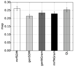
(b) Performance with grid tuning.

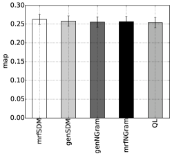
(c) Performance with RankLib.

Figure 3: Experimental evaluation and results

All underlying language models are smoothed with Dirichlet smoothing, as a preliminary study with Jelinek Mercer smoothing yielded worse results. (This finding is consistent with a study of Smucker et al. [15].)

Term probabilities of different language models are on very different scales. Such as is the average probability of bag-of-bigram entry is much smaller than a probability under the unigram model, which is in turn much smaller than a term under a conditional bigram model. As we anticipate that the Dirichlet scale parameter $\mu$ needs to be adjusted we introduce separate parameters for different language models (and not use parameter tying).

7.1 Experimental Setup

Aiming for a realistic collection with rather complete assessments and multi-word queries, we study method performance on the Robust04 test set. The test set contains 249 queries and perform tokenization on whitespace, stemming with Krovetz stemmer, but only remove stopwords for unigram models. While we focus on the measure mean-average precision (MAP), similar results are obtained for ERR@20, R-Precision, bpref, MRR, and P@10 (available upon request).

We use five-fold cross validation using folds that are identical to empirical studies of Huston et al. [8, 9]. The training fold is used to select both the Dirichlet scale parameters $\mu$ and weight parameters $\boldsymbol{\lambda}$. Performance is measured on the test fold only.

Parameters are estimated in two phases. First the Dirichlet scale parameter $\mu$ is selected to maximize retrieval performance (measured in MAP) of each language model individually. See Table 1 for range of the search grid, estimated Dirichlet parameter, and training performance.

In the subsequent phase, Dirichlet parameters are held fixed while the weight parameter $\boldsymbol{\lambda}=\{\lambda_{u},\lambda_{b},\lambda_{w}\}$ is selected. To avoid performance differences due different machine learning algorithms, we evaluate two learning approaches for weight parameter $\boldsymbol{\lambda}$: grid search and coordinate ascent from RankLib. Despite not strictly being necessary, for grid search we only consider nonnegative weights that sum to one, as suggested in the original SDM paper [11]. Each weight entry is selected on a grid $\lambda\in[0.0,0.05,\ldots 0.95,1.0]$ while constraint-violating combinations are discarded. The RankLib experiment does not use a grid, but performs coordinate-ascent with five restarts.

For single-term queries, all discussed approaches reduce to the Query Likelihood model, i.e., unigram model. We therefore hold them out during the training phase, but include them in the test phase, where they obtain the same ranking for all approaches.

Table 1: Dirichlet settings with max MAP on the train set.

split	$\mu_{u}$	MAP	$\mu_{b}$	MAP	$\mu_{w}$	MAP
0	1000	0.252	18750	0.131	20000	0.171
1	1000	0.253	18750	0.127	2500	0.163
2	1000	0.252	18750	0.131	20000	0.165
3	1000	0.254	18750	0.135	20000	0.168
4	1000	0.259	21250	0.130	2500	0.170
$\mu\in[10,250,500,\ldots,2500,3000,3500,\ldots,5000,10000]$

(a) Bag-of-bigram models.

split	$\mu_{u}$	MAP	$\mu_{b}$	MAP	$\mu_{w}$	MAP
0	1000	0.252	5	0.171	1	0.213
1	1000	0.253	5	0.172	1	0.209
2	1000	0.252	5	0.168	1	0.206
3	1000	0.254	5	0.175	1	0.210
4	1000	0.259	5	0.172	1	0.213
$\mu\in[1,5,10,50,100,150,200,250,500,750,1000]$

(b) N-gram models.

Table 2: Selected weight parameter combinations parameter, which are stable across folds, with training MAP. Left: grid tuning; Right: RankLib (Figure 3b shows results on test set).

method	$\lambda_{u}$	$\lambda_{b}$	$\lambda_{w}$	MAP	$\lambda_{u}$	$\lambda_{b}$	$\lambda_{w}$	MAP
mrfSDM	0.85	0.15	0.05	0.26	0.88	0.06	0.06	0.26
genSDM	0.05	0.05	0.9	0.21	0.32	0.45	0.24	0.26
genNGram	0.35	0	0.65	0.23	0.10	0.01	0.89	0.26
$\lambda\in[0.0,0.05,0.10,\dots 0.95,1.0]$					coord ascent

7.2 Empirical Results

The results of the evaluation with standard error bars are presented in Figure 3b for the grid tuning experiment and in Figure 3c for the RankLib experiment.

In the grid-tuning experiment it appears that the MRF-based SDM model is clearly better than any of the other variants, including both generative models as well as the MRF-variant with n-gram features. The second best method is the query likelihood method. However, once $\boldsymbol{\lambda}$ is learned with coordinate ascent from RankLib, the difference disappears. This is concerning, because it may lead to the false belief of discriminative models being superior for this task.

The achieved performance of mrfSDM in both cases is consistent with the results of the experiment conducted by Huston et al. [8].

Generative models

In all cases, weight parameters $\lambda$ and Dirichlet scale parameters $\mu$ selected on the training folds, cf. Tables 1 and 2, are stable across folds.

We observe that selected weight parameterization for the genNGram model puts the highest weight on the windowed bigram model, omitting the bigram model completely. In fact, among all four bigram language models, the n-gram windowed bigram model, described in Section 6.2 achieves the highest retrieval performance by itself (MAP 0.21, column $\mu_{w}$ in Table 1b).

For the genSDM model, which is based on bag-of-bigrams, the weight parameters rather inconsistent across folds and training methods, suggesting that the model is unreliably when trained with cross validation.

Markov random fields

In order to understand whether the success factor of the mrfSDM lies in the log-linear optimization, or in the bag-of-bigram features, we also integrate the n-gram based features discussed in Section 6 as features into the MRF-based SDM algorithm introduced by Metzler et al. (discussed in Section 4). This approach is denoted as mrfNGram in Figure 3b. While the performance is diminished when using grid-tuning, identical performance is achieved when parameters are estimated with RankLib (Figure 3c).

Discussion

We conclude that all four term-dependency methods are able to achieve the same performance, no matter whether a generative approach or a different bigram paradigm is chosen. We also do not observe any difference across levels of difficulty (result omitted). This is not surprising given the similarities between the models, as elaborated in this paper.

However, a crucial factor in this analysis is the use of a coordinate ascent algorithm for selection of weight parameters. The coordinate ascent algorithm was able to find subtle but stable weight combinations that the grid tuning algorithm did not even inspect.

An important take-away is to not rely on grid tuning for evaluating discriminative model in comparison generative models, as it may falsely appear that the discriminative model achieves a significant performance improvement (compare mrfSDM versus genSDM in Figure 3b), where actually this is only due to inabilities of fixed grid-searches to suitably explore the parameter space.

8 Related Work

This work falls into the context of other works that study different common axiomatic paradigms [16] used in information retrieval empirically and theoretically. Chen and Goodman [5] studied different smoothing methods for language modeling, while Zhai and Lafferty [17] re-examine this question for the document retrieval task. Finally, Smucker and Allan [15] concluded which characteristic of Dirichlet smoothing leads to its superiority over Jelinek-Mercer smoothing.

Our focus is on the theoretical understanding of equivalences of different probabilistic models that consider sequential term dependencies, such as [11]. Our work is motivated to complement the empirical comparison of Huston and Croft [8, 9]. Huston and Croft studied the performance of the sequential dependence model and other widely used retrieval models with term dependencies such as BM25-TP, as well as Terrier’s pDFR-BiL2 and pDFR-PL2 with an elaborate parameter tuning procedure with five fold cross validation. The authors found that the sequential dependence model outperforms all other evaluated method with the only exception being an extension, the weighted sequential dependence model [3]. The weighted sequential dependence model extends the feature space for unigrams, bigrams, and windowed bigrams with additional features derived from external sources such as Wikipedia titles, MSN query logs, and Google n-grams.

9 Conclusion

In this work we take a closer look at the theoretical underpinning of the sequential dependence model. The sequential dependence model is derived as a Markov random field, where a common choice for potential functions are log-linear models. We show that the only difference between a generative bag-of-bigram model and the SDM model is that one operates in log-space the other in the space of probabilities. This is where the most important difference between SDM and generative mixture of language models lies.

We confirm empirically, that all four term-dependency models are capable of achieving the same good retrieval performance. However, we observe that grid tuning is not a sufficient algorithm for selecting the weight parameter—however a simple coordinate ascent algorithm, such as obtainable from the RankLib package finds optimal parameter settings. A shocking result is that for the purposes of comparing different models, tuning parameters on an equidistant grid may lead to the false belief that the MRF model is significantly better, where in fact, this is only due to the use of an insufficient parameter estimation algorithm.

This analysis of strongly related models that following the SDM model in spirit, but are based on MRF, generative mixture models, and Jelinek-Mercer/interpolation smoothing might appear overly theoretical. However, as many extensions exist for the SDM model (e.g., including concepts or adding spam features) as well as for generative models (e.g., relevance model (RM3), translation models, or topic models), elaborating on theoretical connections and pinpointing the crucial factors are important for bringing the two research branches together. The result of this work is that, when extending current retrieval models, both the generative and Markov random field framework are equally promising.

Appendix A Approximations in Galago

We noticed some approximations in Galago’s implementation with respect to the bigram and windowed bigram model which also affects the Dirichlet smoothing component. For completeness we discuss these approximations and their effects.

The denominator of both the model and the smoothing term provides a normalizer reflecting counts of ’all possible cases’. In the unigram case, the counts of ’all possible cases’ is the document length $n_{\star,d}=|d|$ and for the smoothing component the collection length $C=n_{\star,\star}=\sum_{d}|d|$.

In the bigram case, the number of all possible bigrams in a document $n_{\left\{\star,\star\right\}_{8},d}=|d|-1\approx|d|$ is approximated in the implementation with the document length. The approximation factors into the smoothing component $n_{\left(\star,\star\right),\star}=\sum_{d}\left(|d|-1\right)=C-\tilde{C}\approx C$ with $\tilde{C}$ denoting the number of documents in the collection. For documents that are long on average, this is a reasonable approximation.

In the windowed-bigram case, all possible windowed bigrams in a document $n_{\left\{q_{i},q_{i+1}\right\}_{8},d}=\left(|d|-7\right)\cdot 28\approx|d|$. This is because the document has $|d|-7$ windows, each with 8 choose 2 cases. The approximation of off by a factor of 28. This also affects the smoothing component, $n_{\left\{\star,\star\right\}_{8},\star}\approx\left(C-7\tilde{C}\right)\cdot 28\approx C$. However, when the smoothing parameter $\mu$ is tuned with relevance data, the constant factor of 28 is absorbed by $\mu$.

References

- [1] M. Bendersky and W. B. Croft. Modeling higher-order term dependencies in information retrieval using query hypergraphs. In SIGIR, pages 941–950, 2012.
- [2] M. Bendersky, W. B. Croft, and Y. Diao. Quality-biased ranking of web documents. In WSDM, pages 95–104, 2011.
- [3] M. Bendersky, D. Metzler, and W. B. Croft. Learning concept importance using a weighted dependence model. In WSDM, pages 31–40, 2010.
- [4] J. P. Callan, W. B. Croft, and J. Broglio. Trec and tipster experiments with inquery. Information Processing & Management, 31(3):327–343, 1995.
- [5] S. F. Chen and J. Goodman. An empirical study of smoothing techniques for language modeling. In ACL, pages 310–318, 1996.
- [6] J. Dalton and L. Dietz. A neighborhood relevance model for entity linking. In RIAO-OAIR, pages 149–156, 2013.
- [7] L. Dietz. Directed factor graph notation for generative models. Technical report, 2010.
- [8] S. Huston and W. B. Croft. A comparison of retrieval models using term dependencies. In WSDM, pages 111–120, 2013.
- [9] S. Huston and W. B. Croft. Parameters learned in the comparison of retrieval models using term dependencies. Technical report, 2014.
- [10] T. Joachims. Optimizing search engines using clickthrough data. In KDD, pages 133–142, 2002.
- [11] D. Metzler and W. B. Croft. A markov random field model for term dependencies. In SIGIR, pages 472–479, 2005.
- [12] D. Metzler and W. B. Croft. Latent concept expansion using markov random fields. In SIGIR, pages 311–318, 2007.
- [13] K. P. Murphy. Machine learning: a probabilistic perspective. MIT press, 2012.
- [14] C. Siefkes, F. Assis, S. Chhabra, and W. S. Yerazunis. Combining winnow and orthogonal sparse bigrams for incremental spam filtering. In PKDD, pages 410–421. 2004.
- [15] M. Smucker and J. Allan. An investigation of dirichlet prior smoothing’s performance advantage. Technical report, 2006.
- [16] C. Zhai. Axiomatic analysis and optimization of information retrieval models. In Conference on the Theory of Information Retrieval, pages 1–1. Springer, 2011.
- [17] C. Zhai and J. Lafferty. A study of smoothing methods for language models applied to ad hoc information retrieval. In SIGIR, pages 334–342, 2001.