Nonlinear quantum optics for spinor slow light

Abstract

We investigate quantum nonlinear effects at a level of individual quanta in a double tripod atom-light coupling scheme involving two atomic Rydberg states. In such a scheme the slow light coherently coupled to strongly interacting Rydberg states represents a two-component or spinor light. The scheme provides additional possibilities for the control and manipulation of light quanta. A distinctive feature of the proposed setup is that it combines the spin-orbit coupling for the spinor slow light with an interaction between the photons, enabling generation of the second probe beam even when two-photon detuning is zero. Furthermore, the interaction between the photons can become repulsive if the one-photon detunings have opposite signs. This is different from a single ladder atom-light coupling scheme, in which the interaction between the photons is attractive for both positive and negative detunings, as long as the Rabi frequency of the control beam is not too large.

I Introduction

Atoms excited to high-lying Rydberg states with a principal quantum number $n$ above 50 have recently attracted a significant attention Saffman et al. (2010). Since the van der Waals interaction between atoms increases with the principal quantum number as $n^{11}$ , the interaction between the Rydberg atoms is enhanced by many orders of magnitude compared to the interaction between atoms in the ground state Bohlouli-Zanjani et al. (2007); Béguin et al. (2013). The strong interaction between the Rydberg atoms prevents a simultaneous excitation of nearby atoms leading to the Rydberg blockade Tong et al. (2004); Singer et al. (2004); Heidemann et al. (2007). These properties of the Rydberg atoms have found application in the quantum information processing Jaksch et al. (2000); Lukin et al. (2001); Gaëtan et al. (2009); Urban et al. (2009); Isenhower et al. (2010), studies of interacting many-body systems Cinti et al. (2010); Pohl et al. (2010); Pupillo et al. (2010); Viteau et al. (2011); Carr et al. (2013); Schauss et al. (2015), as well as non-linear quantum optics for slow light Petrosyan et al. (2011); Gorshkov et al. (2011); Dudin and Kuzmich (2012); Dudin et al. (2012); Peyronel et al. (2012); Firstenberg et al. (2013); Li et al. (2013); Chang et al. (2014). The latter application is based on the fact that the Rydberg interaction brings neighboring Rydberg atoms out of the resonance destroying the electromagnetically induced transparency (EIT). Consequently the closeby Rydberg atoms absorb the slow light which becomes anti-bunched during its propagation through the atomic medium Petrosyan et al. (2011); Gorshkov et al. (2011); Dudin and Kuzmich (2012); Dudin et al. (2012); Peyronel et al. (2012); Firstenberg et al. (2013); Li et al. (2013); Chang et al. (2014). Dispersive coupling of light to strongly interacting atoms in highly excited Rydberg states allows to induce an effective attractive force between the propagating Rydberg polaritons and to create bound states of the polaritons Firstenberg et al. (2013); Bienias et al. (2014). For a recent review of nonlinear quantum optics mediated by Rydberg interactions see Ref. Firstenberg et al. (2016).

In a usual Rydberg EIT, a ladder atom-light coupling configuration is typically employed involving an atomic ground state, an intermediate excited state and a Rydberg state Gorshkov et al. (2011); Peyronel et al. (2012). In the present paper we study a more complicated double tripod level scheme for the Rydberg EIT, providing new physical effects not present in the ladder scheme. The double tripod scheme involves two probe laser fields and there are two adiabatic eigenmodes propagating inside the atomic medium that are imune to spontaneous decay. They form a two-component (spinor) slow light. In the case of non-interacting atoms the propagation of the two-component slow light was considered in Refs. Unanyan et al. (2010); Ruseckas et al. (2011, 2013) and was experimentally demonstrated recently Lee et al. (2014). The double tripod atom-light coupling scheme provides a possibility to create the spin-orbit coupling for the spinor slow light. The influence of the spin-orbit coupling on the propagation of light have been investigated in several studies Bérard and Mohrbach (2004); Bliokh and Bliokh (2004a, b); Onoda et al. (2004); Bérard and Mohrbach (2006) leading to a generalization of geometric optics called geometric spintronics Duval et al. (2006, 2007). The present study adds the interaction effects to the spinor slow light.

Here we include interactions between the atoms excited to the Rydberg levels leading to non-linear effects for the spinor slow light. In contrast to a ladder scheme where a single one-photon detuning can be present, the probe beams in the double tripod setup can have different one-photon detunings. We show that the propagation of the slow light significantly depend not only on the magnitude of one-photon detunings, but also on the their difference. For large and equal one-photon detunings the propagation of the spinor slow light combines a spin-orbit coupling at the distances between photons larger than the Rydberg blockade radius together with an effective attractive interaction of photons at small distances. The latter attractive force is the same as in a ladder scheme used in Ref. Firstenberg et al. (2013). Yet, if the one-photon detunings have opposite signs, the photons from the different probe beams experience repulsion instead of attraction.

Different from a simple ladder scheme, in the double-tripod setup the photons can be transferred from one probe beam to another. Although such a transfer is possible in a double-tripod setup without atom-atom interactions, this can be accomplished only for a nonzero two-photon detuning Ruseckas et al. (2013); Lee et al. (2014). In this paper we show that the interactions between Rydberg atoms together with the spin-orbit coupling makes it possible the second probe beam to appear even when two-photon detuning is zero and the envelope of the input probe field is constant most of the time.

Note, that some of the phenomena considered here can be explored in simpler setups. For example, conversion between the two probe beams can be achieved in double-Lambda linkage pattern involving only one Rydberg level. However, in the double tripod setup there are two adiabatic eigenmodes immune to spontaneous decay, whereas in the double-Lambda setup there is only one. Two adiabatic eigenmodes are needed to create a slow ligtht polariton that behaves as a spinor-like object and is subjected to a spin-orbit coupling. To achieve this, simpler settings are not sufficient.

The proposed double-tripod scheme with Rydberg levels could be a suitable system to explore many-body effects involving the spin-orbit coupling. The setup can also lead to novel applications in quantum information manipulation and nonlinear optics. For example, this scheme can be used to realize the quantum gates for two-color qubits, where two-color qubit represents a superposition state of two frequency modes. Conversion between different probe photons caused by Rydberg interactions can be utilized for generation of a second photon of different frequency entangled with the photon incident on the medium.

The paper is organized as follows. In Sec. II we present the proposed setup and in Sec. III we introduce a description of the system. In Sec. IV we consider the case when both one-photon detunings are equal and derive an approximate closed propagation equation for the two-photon wave function. In Sec. V we investigate the consequences of one-photon detunings having the opposite signs. Section VI summarizes the findings.

II Formulation

II.1 Atom-light system

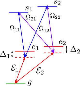
Figure 1: Double tripod atom-light coupling scheme involving the ground level $g$, the Rydberg levels $s_{1}$ and $s_{2}$, and the intermediate excited levels $e_{1}$ and $e_{2}$. Two weak probe beams with the amplitudes $\mathcal{E}_{j}$ connect the ground level $g$ to the intermediate levels $e_{j}$. Four strong control beam with the Rabi frequencies $\Omega_{jl}$ connect the intermediate levels $e_{j}$ to the Rydberg levels $s_{j}$.

Let us consider an ensemble of atoms characterized by a double tripod scheme of energy levels shown in Fig. 1. The scheme includes an atomic ground level $g$, Rydberg levels $s_{1}$, $s_{2}$, and intermediate excited levels $e_{1}$, $e_{2}$, the corresponding energies being $\hbar\omega_{g}$, $\hbar\omega_{s_{j}}$ and $\hbar\omega_{e_{j}}$ ($j=1,2$). We assume that the levels $s_{1}$ and $s_{2}$ are both Rydberg $s$ or $d$ states. The atoms interact with two probe laser fields of lower intensities and four control fields of much higher intensities. The probe fields with central frequencies $\omega_{p_{j}}$ drive the atomic transitions $g\rightarrow e_{j}$. The control fields characterized by the frequencies $\omega_{c_{j,l}}$ couple the atomic transitions $e_{j}\rightarrow s_{l}$ ($j=1,2$; $l=1,2$) with the coupling strengths characterized by the Rabi frequencies $\Omega_{j,l}$.

To simplify the description we consider a narrow cigar shape atom cloud. As in the previously considered latter scheme Peyronel et al. (2012); Firstenberg et al. (2013), the atomic density is assumed to be constant across the probe beams and the Rydberg blockade radius is larger than the waists of the beams. In such a situation a one-dimensional approximation is suitable for the description of the propagating probe fields. In the continuum approximation Fleischhauer and Lukin (2002); Gorshkov et al. (2011) the probe fields and atomic excitations can be represented by slowly varying operators $\hat{\mathcal{E}}_{j}^{{\dagger}}(z)$, $\hat{\Psi}_{e_{j}}^{{\dagger}}(z)$ and $\hat{\Psi}_{s_{j}}^{{\dagger}}(z)$. The former $\hat{\mathcal{E}}_{j}^{{\dagger}}(z)$ describes the creation at the position $z$ of a photon with the frequency $\omega_{p_{j}}$. The latter material operators $\hat{\Psi}_{e_{j}}^{{\dagger}}(z)$ and $\hat{\Psi}_{s_{j}}^{{\dagger}}(z)$ describe excitation of the intermediate electronic level $e_{j}$ and the Rydberg level $s_{j}$, respectively. In the Heisenberg representation, the field operators obey the equal-time commutation relations

$$[\hat{\mathcal{E}}_{j}(z,t),\hat{\mathcal{E}}_{j}^{{\dagger}}(z^{\prime},t)]=[\hat{\Psi}_{e_{j}}(z,t),\hat{\Psi}_{e_{j}}^{{\dagger}}(z^{\prime},t)]=[\hat{\Psi}_{s_{j}}(z,t),\hat{\Psi}_{s_{j}}^{{\dagger}}(z^{\prime},t)]=\delta(z-z^{\prime})\,,$$ (1)

all other equal time commutators being zero.

Outside the medium the Heisenberg equation of motion for the slowly varying probe field reads

$$\partial_{t}\hat{\mathcal{E}}_{j}(z,t)=-c\partial_{z}\hat{\mathcal{E}}_{j}(z,t)\,.$$ (2)

Inside the medium the Heisenberg equations of motion for the annihilation operators have a form similar to the ones previously considered for three level $\Lambda$ or ladder schemes Fleischhauer and Lukin (2002); Gorshkov et al. (2007, 2011)

$$\partial_{t}\hat{\mathcal{E}}_{j}(z,t) =-c\partial_{z}\hat{\mathcal{E}}_{j}(z,t)+i\frac{g}{2}\hat{\Psi}_{e_{j}}(z,t)\,,$$ (3)

$$\partial_{t}\hat{\Psi}_{e_{j}}(z,t) =-\frac{i}{2}\tilde{\Delta}_{j}\hat{\Psi}_{e_{j}}(z,t)+i\frac{g}{2}\hat{\mathcal{E}}_{j}(z,t)+\frac{i}{2}\sum_{l}\Omega_{jl}\hat{\Psi}_{s_{l}}(z,t)\,,$$ (4)

$$\partial_{t}\hat{\Psi}_{s_{j}}(z,t) =\frac{i}{2}\sum_{l}\Omega_{l,j}^{*}\hat{\Psi}_{e_{l}}(z,t)-i\hat{U}(z,t)\hat{\Psi}_{s_{j}}(z,t)\,.$$ (5)

with

$$\tilde{\Delta}_{j}=2\Delta_{j}-i\Gamma_{j}\,.$$ (6)

To include decay of excited states $e_{j}$ with rates $\Gamma_{j}$, we have added an imaginary part to the one photon detunings $\Delta_{j}=\omega_{e_{j}}-\omega_{g}-\omega_{p_{j}}$ replacing the latter by the complex-valued quantities $\tilde{\Delta}_{j}$ featured in Eq. (4). In the following for simplicity we will assume that $\Gamma_{j}=\Gamma$ is the same for both levels. In Eq. (5) we have neglected the decay of a coherence between the ground $g$ and Rydberg $s_{j}$ states. In Eqs. (4)–(5) the two-photon detunings are taken to be zero, $\omega_{g}+\omega_{p_{j}}+\omega_{c_{j,l}}-\omega_{s_{l}}=0$, yet the one-photon detunings $\Delta_{j}$ are generally nonzero. In Eqs. (3) and (4) the parameter $g$ characterizes the atom-photon coupling strength and is assumed the same for both probe fields. The coupling strength $g$ is related to the optical density $\alpha$ of the medium via the equation $g^{2}=c\Gamma\alpha/L$, where $L$ is the length of the medium which extends from $z=0$ to $z=L$. Finally, the operator

$$\hat{U}(z,t)=\int dz^{\prime}\,V(z-z^{\prime})\sum_{j}\hat{\Psi}_{s_{j}}^{{\dagger}}(z^{\prime},t)\hat{\Psi}_{s_{j}}(z^{\prime},t)$$ (7)

describes the interaction between the Rydberg atoms. This expression for the operator $\hat{U}(z,t)$ represents only the density-density interaction between the Rydberg states, corresponding to the van der Waals interaction. In general, the exchange interaction between the Rydberg states can also be present Li et al. (2014); Gorniaczyk et al. (2016). The exchange interaction strength is significant only when the difference between the principal quantum numbers is equal to 1 and becomes much smaller for larger differences van Bijnen (2013). In the present study we assume that the difference between the principal quantum numbers of the Rydberg levels is sufficiently large so that the exchange interaction can be neglected. Similarly to the exchange interaction, the energy exchange between atoms can also occur due to the resonant dipole-dipole interaction (RDDI). Yet the latter RDDI does not show up when both Rydberg states are the $s$ or $d$ states due to the vanishing interaction matrix element, as it is the case in the situation considered here. For simplicity the position-dependent interaction strength $V(z)=C_{6}/z^{6}$ is taken to be the same for the atoms in both Rydberg levels $s_{1}$ and $s_{2}$ in Eq. (7). Such an assumption is justified when the difference between the principal quantum numbers of both Rydberg levels is not too large. This and the previously mentioned restrictions can co-exisit e.g. by taking a difference in the principal quantum numbers to be around 3 to 5. The interaction potential $V(r)$ defines the Rydberg blockade radius $r_{\mathrm{b}}$ via the equality

$$V(r_{\mathrm{b}})=\Omega^{2}/\Gamma\,,$$ (8)

where $\Omega$ is the maximum Rabi frequency of the control beams. Note that in Eqs. (3)–(5) we have omitted the Langevin noise due to the spontaneous emission Scully and Zubairy (1997), because it is not important for our analysis involving a low number of excitations Gorshkov et al. (2013).

II.2 Two excitation wave-functions

Similar to the previously considered propagation of a single probe beam Peyronel et al. (2012); Firstenberg et al. (2013), the probe fields are assumed to be sufficiently weak at the input, so that the contribution due to more than two photons is not important. The initial state $|\Phi\rangle$ of the the quantized radiation field and atomic excitations can then be written only in terms of components containing at most two photons. Envelopes of input probe pulses are assumed to be long and flat. Thus, except for a short transient period, the envelopes can be considered to be constant most of the time.

The temporal evolution of the Heisenberg operators (3)–(5) preserves the total number of photons and atomic excitations. The radiation fields and atomic excitations originating from a single photon input are not subjected to the atom-atom interactions and propagate through the EIT medium without a decay. In the single-particle picture, the propagation of the two-component (spinor) slow light in the double tripod system has been investigated theoretically Unanyan et al. (2010); Ruseckas et al. (2011, 2013) and experimentally Lee et al. (2014). It has been shown that propagation of the slow light in the double tripod system causes oscillations between the two probe fields inside the medium. The oscillations can be described by introducing a matrix of the group velocity with the matrix elements given by Ruseckas et al. (2013)

$$v_{j,l}=\frac{c}{g^{2}}\sum_{m}\Omega_{j,m}\Omega_{l,m}^{*}\,.$$ (9)

Note, that when the interactions between atoms are present, the condition for the EIT can be violated. However, we will use the group velocty matrix (9) as a convenient quantity describing the evolution of the two-excitation state.

Here we are interested in the two-excitation wave functions Hafezi et al. (2012) for the double tripod scheme. They are defined as

$$\Phi_{\mathcal{E}_{j}\mathcal{E}_{l}}(z,z^{\prime},t) = \langle\mathrm{vac}|\hat{\mathcal{E}}_{j}(z,t)\hat{\mathcal{E}}_{l}(z^{\prime},t)|\Phi\rangle\,,$$ (10)

$$\Phi_{\mathcal{E}_{j}s_{l}}(z,z^{\prime},t) = \langle\mathrm{vac}|\hat{\mathcal{E}}_{j}(z,t)\hat{\Psi}_{s_{l}}(z^{\prime},t)|\Phi\rangle\,,$$ (11)

$$\Phi_{s_{j}s_{l}}(z,z^{\prime},t) = \langle\mathrm{vac}|\hat{\Psi}_{s_{j}}(z,t)\hat{\Psi}_{s_{l}}(z^{\prime},t)|\Phi\rangle\,,$$ (12)

where $|\Phi\rangle$ is an initial state of the system comprising the quantized radiation field and atomic excitations. Since the total number of excitations is preserved during the temporal evolution, only the two photon part of the initial state-vector $|\Phi\rangle$ contributes to the wave-functions (10)–(12). Using Eqs. (3)–(5), in the following Section we will obtain the equations governing the two-excitation wave functions (10)–(12) inside the medium.

III Approximate equations for two-excitation wave functions

In this section we will obtain an approximate equations describing the propagation of the probe fields inside the medium. To simplify the equations we eliminate the intermediate electronic excited levels $e_{j}$ from the description, assuming that the decay rate $\Gamma$ or the one-photon detuning $\Delta_{j}$ are large compared to $g$ or $\Omega_{j,l}$. Adiabatic elimination of an intermediate level to describe the propagation of Rydberg polariton in a ladder scheme has been used in Ref. Gorshkov et al. (2011). We expand all operators in the power series of $\tilde{\Delta}_{j}^{-1}$ powers: $\hat{\mathcal{X}}=\hat{\mathcal{X}}^{(0)}+\hat{\mathcal{X}}^{(1)}+\cdots$ , subject to the initial condition $\hat{\mathcal{X}}(z,0)=\hat{\mathcal{X}}^{(0)}(z,0)$ at $t=0$. Here $\hat{\mathcal{X}}$ stands for the operators $\hat{\mathcal{E}}_{j}$, $\hat{\Psi}_{e_{j}}$ , $\hat{\Psi}_{s_{j}}$. Collecting the terms of the same size in Eq. (4) we obtain that the operator $\hat{\Psi}_{e_{j}}^{(0)}$ obeys the equation

$$\partial_{t}\hat{\Psi}_{e_{j}}^{(0)}=-\frac{i}{2}\tilde{\Delta}_{j}\hat{\Psi}_{e_{j}}^{(0)}$$ (13)

and thus rapidly changes in time: $\hat{\Psi}_{e_{j}}^{(0)}(t)=\hat{\Psi}_{e_{j}}(0)\exp(-i\tilde{\Delta}_{j}t/2)$. The first-order terms in Eq. (4) lead to the following expression for the slowly changing part $\hat{\Psi}_{e_{j}}^{(1)}$:

$$\hat{\Psi}_{e_{j}}^{(1)}=\tilde{\Delta}_{j}^{-1}g\hat{\mathcal{E}}_{j}^{(0)}+\tilde{\Delta}_{j}^{-1}\sum_{l}\Omega_{j,l}\hat{\Psi}_{s_{l}}^{(0)}\,.$$ (14)

Inserting this expression into Eqs. (3), (5) we get the equations for the slowly changing operators

$$\partial_{t}\hat{\mathcal{E}}_{j} =-c\partial_{z}\hat{\mathcal{E}}_{j}+i\frac{g^{2}}{2}\tilde{\Delta}_{j}^{-1}\hat{\mathcal{E}}_{j}+i\frac{g}{2}\tilde{\Delta}_{j}^{-1}\sum_{l}\Omega_{j,l}\hat{\Psi}_{s_{l}}\,,$$ (15)

$$\partial_{t}\hat{\Psi}_{s_{j}} =i\frac{g}{2}\sum_{l}\tilde{\Delta}_{l}^{-1}\Omega_{l,j}^{*}\hat{\mathcal{E}}_{l}+\frac{i}{2}\sum_{l,m}\Omega_{l,j}^{*}\tilde{\Delta}_{l}^{-1}\Omega_{l,m}\hat{\Psi}_{s_{m}}-i\hat{U}\hat{\Psi}_{s_{j}}\,,$$ (16)

where we have dropped the upper index $(0)$ for a brevity. Using the definitions of the two-excitation wave functions (10)–(12) and Eqs. (15), (16) we obtain the following propagation equations:

$$\partial_{t}\Phi_{\mathcal{E}_{j}\mathcal{E}_{l}}= -c(\partial_{z}+\partial_{z^{\prime}})\Phi_{\mathcal{E}_{j}\mathcal{E}_{l}}+i\frac{g^{2}}{2}(\tilde{\Delta}_{j}^{-1}+\tilde{\Delta}_{l}^{-1})\Phi_{\mathcal{E}_{j}\mathcal{E}_{l}}$$

$$+i\frac{g}{2}\sum_{m}(\tilde{\Delta}_{l}^{-1}\Omega_{l,m}\Phi_{\mathcal{E}_{j}s_{m}}+\tilde{\Delta}_{j}^{-1}\Omega_{j,m}\Phi_{s_{m}\mathcal{E}_{l}})\,,$$ (17)

$$\partial_{t}\Phi_{\mathcal{E}_{j}s_{l}}= -c\partial_{z}\Phi_{\mathcal{E}_{j}s_{l}}+i\frac{g^{2}}{2}\tilde{\Delta}_{j}^{-1}\Phi_{\mathcal{E}_{j}s_{l}}+\frac{i}{2}\sum_{m,n}\Omega_{m,l}^{*}\tilde{\Delta}_{m}^{-1}\Omega_{m,n}\Phi_{\mathcal{E}_{j}s_{n}}$$

$$+i\frac{g}{2}\sum_{m}\left(\tilde{\Delta}_{m}^{-1}\Omega_{m,l}^{*}\Phi_{\mathcal{E}_{j}\mathcal{E}_{m}}+\tilde{\Delta}_{j}^{-1}\Omega_{j,m}\Phi_{s_{m}s_{l}}\right)\,,$$ (18)

$$\partial_{t}\Phi_{s_{j}s_{l}}= i\frac{g}{2}\sum_{m}\tilde{\Delta}_{m}^{-1}(\Omega_{m,j}^{*}\Phi_{\mathcal{E}_{m}s_{l}}+\Omega_{m,l}^{*}\Phi_{s_{j}\mathcal{E}_{m}})+\frac{i}{2}\sum_{m,n}\tilde{\Delta}_{m}^{-1}\Omega_{m,n}(\Omega_{mj}^{*}\Phi_{s_{n}s_{l}}+\Omega_{m,l}^{*}\Phi_{s_{j}s_{n}})$$

$$-iV(z^{\prime}-z)\Phi_{s_{j}s_{l}}\,.$$ (19)

The envelopes of the input probe fields are assumed to be constant most of the time, so the boundary conditions for Eqs. (17)–(19) are time independent. Hence one can consider the steady state of the fields by dropping the time derivatives in Eqs. (17)–(19). To simplify the equations it is convenient to introduce the following combinations of two-excitation wave functions:

$$\Phi_{j,l}^{\mathcal{E}s}(z,z^{\prime}) =\frac{1}{g}\sum_{m}\Omega_{lm}\Phi_{\mathcal{E}_{j}s_{m}}(z,z^{\prime})\,,$$ (20)

$$\Phi_{j,l}^{s\mathcal{E}}(z,z^{\prime}) =\frac{1}{g}\sum_{m}\Omega_{jm}\Phi_{s_{m}\mathcal{E}_{l}}(z,z^{\prime})\,,$$ (21)

$$\Phi_{j,l}^{ss}(z,z^{\prime}) =\frac{1}{g^{2}}\sum_{m,n}\Omega_{jm}\Omega_{ln}\Phi_{s_{m}s_{n}}(z,z^{\prime})\,.$$ (22)

Calling on Eqs. (17)–(19), one arrives at the steady state equations for the combined wave functions $\Phi_{j,l}^{\mathcal{E}s}$, $\Phi_{j,l}^{s\mathcal{E}}$ and $\Phi_{j,l}^{ss}$:

$$0 =-c(\partial_{z}+\partial_{z^{\prime}})\Phi_{\mathcal{E}_{j}\mathcal{E}_{l}}+i\frac{g^{2}}{2}\left((\tilde{\Delta}_{j}^{-1}+\tilde{\Delta}_{l}^{-1})\Phi_{\mathcal{E}_{j}\mathcal{E}_{l}}+\tilde{\Delta}_{l}^{-1}\Phi_{j,l}^{\mathcal{E}s}+\tilde{\Delta}_{j}^{-1}\Phi_{j,l}^{s\mathcal{E}}\right)\,,$$ (23)

$$0 =-c\partial_{z}\Phi_{j,l}^{\mathcal{E}s}+i\frac{g^{2}}{2}\tilde{\Delta}_{j}^{-1}(\Phi_{j,l}^{\mathcal{E}s}+\Phi_{j,l}^{ss})+i\frac{g^{2}}{2}\sum_{m}\tilde{\Delta}_{m}^{-1}\frac{v_{l,m}}{c}(\Phi_{j,m}^{\mathcal{E}s}+\Phi_{\mathcal{E}_{j}\mathcal{E}_{m}})\,,$$ (24)

$$0 =-c\partial_{z^{\prime}}\Phi_{j,l}^{s\mathcal{E}}+i\frac{g^{2}}{2}\tilde{\Delta}_{l}^{-1}(\Phi_{j,l}^{s\mathcal{E}}+\Phi_{j,l}^{ss})+i\frac{g^{2}}{2}\sum_{m}\tilde{\Delta}_{m}^{-1}\frac{v_{j,m}}{c}(\Phi_{m,l}^{s\mathcal{E}}+\Phi_{\mathcal{E}_{m}\mathcal{E}_{l}})\,,$$ (25)

$$0 =\sum_{m}\tilde{\Delta}_{m}^{-1}\left(v_{j,m}(\Phi_{m,l}^{\mathcal{E}s}+\Phi_{m,l}^{ss})+v_{l,m}(\Phi_{j,m}^{s\mathcal{E}}+\Phi_{j,m}^{ss})\right)-\frac{2c}{g^{2}}V(z^{\prime}-z)\Phi_{j,l}^{ss}\,,$$ (26)

Here the Rabi frequencies enter only via the matrix elements $v_{j,l}$ of the the group velocity matrix, defined by Eq. (9). Numerical solution of Eqs. (23)–(26) for various values of the one-photon detunings $\Delta_{1}$ and $\Delta_{2}$ shows that the wave function $\Phi_{\mathcal{E}_{j}\mathcal{E}_{l}}$ can be approximated as

$$\Phi_{\mathcal{E}_{j}\mathcal{E}_{l}}=-\frac{1}{2}(\Phi_{j,l}^{\mathcal{E}s}+\Phi_{j,l}^{s\mathcal{E}})\,.$$ (27)

The last term in Eqs. (24) and (25) contains the ratio of the group velocity to the speed of light $v/c$. Under the EIT conditions the group velocity $v$ is much smaller than the speed of light, $v/c\ll 1$, so we neglect the last term in Eqs. (24) and (25), giving

$$0 =-c\partial_{z}\Phi_{j,l}^{\mathcal{E}s}+i\frac{g^{2}}{2}\tilde{\Delta}_{j}^{-1}(\Phi_{j,l}^{\mathcal{E}s}+\Phi_{j,l}^{ss})\,,$$ (28)

$$0 =-c\partial_{z^{\prime}}\Phi_{j,l}^{s\mathcal{E}}+i\frac{g^{2}}{2}\tilde{\Delta}_{l}^{-1}(\Phi_{j,l}^{s\mathcal{E}}+\Phi_{j,l}^{ss})\,.$$ (29)

To get a closed equation we need to solve Eq. (26) to express the wave functions $\Phi_{j,l}^{ss}$ via $\Phi_{j,l}^{\mathcal{E}s}$ and $\Phi_{j,l}^{s\mathcal{E}}$. As it is shown in the Appendix A, the solution of Eq. (26) can be written in the following form:

$$\Phi_{j,l}^{ss}+\Phi_{j,l}^{\mathcal{E}s+}=\frac{1}{\tilde{\Delta}_{1}^{-1}v_{1,1}+\tilde{\Delta}_{2}^{-1}v_{2,2}-\frac{2c}{g^{2}}V(z^{\prime}-z)}\left(\sum_{m}\tilde{\Delta}_{m}^{-1}(v_{l,m}\Phi_{j,m}^{\mathcal{E}s-}-v_{j,m}\Phi_{m,l}^{\mathcal{E}s-})\right.\\ \left.-\frac{2c}{g^{2}}V(z^{\prime}-z)\sum_{m,n}A_{j,l;m,n}\Phi_{m,n}^{\mathcal{E}s+}\right)\,,$$ (30)

where

$$\Phi_{j,l}^{\mathcal{E}s+} =\frac{1}{2}(\Phi_{j,l}^{\mathcal{E}s}+\Phi_{j,l}^{s\mathcal{E}})\,,$$ (31)

$$\Phi_{j,l}^{\mathcal{E}s-} =\frac{1}{2}(\Phi_{j,l}^{\mathcal{E}s}-\Phi_{j,l}^{s\mathcal{E}})\,.$$ (32)

Note that the wave functions $\Phi_{j,l}^{\mathcal{E}s+}$ and $\Phi_{j,l}^{\mathcal{E}s-}$ represent a generalization of the symmetric and antisymmetric combinations of two-excitation wave functions used in Ref. Peyronel et al. (2012) for a simpler ladder scheme. The coefficients $A_{j,l;m,n}$ in Eq. (30) are obtained from the solution of linear equations (58) written in the form (60). We do not present analytical expressions for the coefficients $A_{j,l;m,n}$ explicitly, since these expressions are long and not informative.

IV Equal one-photon detunings

IV.1 Closed equation for the two-photon wave function

In this Section we will consider the case of equal one-photon detunings, $\Delta_{1}=\Delta_{2}\equiv\Delta$. In this situation one can obtain a closed approximate equation for the two-photon wave function. To do this we will employ of the center of mass and relative coordinates

$$R=\frac{1}{2}(z+z^{\prime})\,,\qquad r=z-z^{\prime}\,.$$ (33)

Note, that $R$ and $r$ form a pair of mutually indepent coordinates that can be used instead of the initial coordinates $z$ and $z^{\prime}$. Using the center of mass and relative coordinates, Eqs. (28), (29) for the combined wave functions $\Phi_{j,l}^{\mathcal{E}s+}$, $\Phi_{j,l}^{\mathcal{E}s-}$ become

$$0 =-\frac{c}{2}\partial_{R}\Phi_{j,l}^{\mathcal{E}s+}-c\partial_{r}\Phi_{j,l}^{\mathcal{E}s-}+i\frac{g^{2}}{2}\tilde{\Delta}^{-1}(\Phi_{j,l}^{\mathcal{E}s+}+\Phi_{j,l}^{ss})\,,$$ (34)

$$0 =-\frac{c}{2}\partial_{R}\Phi_{j,l}^{\mathcal{E}s-}-c\partial_{r}\Phi_{j,l}^{\mathcal{E}s+}+i\frac{g^{2}}{2}\tilde{\Delta}^{-1}\Phi_{j,l}^{\mathcal{E}s-}\,.$$ (35)

The symmetric combination $\Phi_{j,l}^{\mathcal{E}s+}$ enters the last term of equation (23) and is thus directly coupled to $\Phi_{\mathcal{E}_{j}\mathcal{E}_{l}}$. The antisymmetric combination $\Phi_{j,l}^{\mathcal{E}s-}$ is decoupled from $\Phi_{j,l}^{ss},$ as one can see in the equation (35) for $\Phi_{j,l}^{\mathcal{E}s-}$ . We next simplify Eqs. (34)–(35) using several approximations, similar to the ones employed in Refs. Peyronel et al. (2012); Firstenberg et al. (2013). In Eq. (35) we neglect the spatial derivative $\partial_{R}\Phi_{j,l}^{\mathcal{E}s-}$, thus relating $\Phi_{j,l}^{\mathcal{E}s-}$ to $\Phi_{j,l}^{\mathcal{E}s+}$:

$$\Phi_{j,l}^{\mathcal{E}s-}=-2i\frac{c}{g^{2}}\tilde{\Delta}\partial_{r}\Phi_{j,l}^{\mathcal{E}s+}\,.$$ (36)

Inserting Eq. (36) into Eq. (34) and using Eq. (30) together with Eq. (27) one arrives at a closed equation for the two-photon wave functions

$$i\partial_{R}\Phi_{\mathcal{E}_{j}\mathcal{E}_{l}}=-4L_{\mathrm{abs}}\frac{\tilde{\Delta}}{\Gamma}\partial_{r}^{2}\Phi_{\mathcal{E}_{j}\mathcal{E}_{l}}+\frac{i}{\bar{v}-L_{\mathrm{abs}}\frac{\tilde{\Delta}}{\Gamma}V(r)}\sum_{m}(v_{l,m}\partial_{r}\Phi_{\mathcal{E}_{j}\mathcal{E}_{m}}-v_{j,m}\partial_{r}\Phi_{\mathcal{E}_{m}\mathcal{E}_{l}})\\ +\frac{V(r)}{\bar{v}-L_{\mathrm{abs}}\frac{\tilde{\Delta}}{\Gamma}V(r)}\sum_{m,n}A_{jl,mn}\Phi_{\mathcal{E}_{m}\mathcal{E}_{n}}\,.$$ (37)

Here

$$\bar{v}=\frac{1}{2}(v_{1,1}+v_{2,2})$$ (38)

is the average group velocity and

$$L_{\mathrm{abs}}=\frac{L}{\alpha}$$ (39)

is a resonant absorption length.

Equation (37), describing the propagation of two probe photons in the medium, reveals several physical effects occurring during such a propagation. Compared to a ladder scheme typically used for Rydberg EIT Peyronel et al. (2012); Firstenberg et al. (2013), the double tripod setup, considered in this paper, has more tunable parameters. There are two limiting cases of Eq. (37) corresponding to large and small separation $r$ between two photons (compared to the Rydberg blockade radius). For separation distances $r$ much larger than the blockade radius, the interaction potential $V(r)$ vanishes and Eq. (37) reduces to

$$i\partial_{R}\Phi_{\mathcal{E}_{j}\mathcal{E}_{l}}=-4L_{\mathrm{abs}}\left(\frac{2\Delta}{\Gamma}-i\right)\partial_{r}^{2}\Phi_{\mathcal{E}_{j}\mathcal{E}_{l}}+\frac{i}{\bar{v}}\sum_{m}(v_{l,m}\partial_{r}\Phi_{\mathcal{E}_{j}\mathcal{E}_{m}}-v_{j,m}\partial_{r}\Phi_{\mathcal{E}_{m}\mathcal{E}_{l}})\,.$$ (40)

When the one-photon detuning is large compared to the rate of the excited state delay, $\Delta\gg\Gamma$, Eq. (40) has the form of a Schrödinger equation where the center of mass coordinate $R$ plays a role of “time” and the relative coordinate $r$ enters as a “spatial coordinate”. The first term on the right hand side of Eq. (40) represents the kinetic energy corresponding to an effective mass $\tilde{m}=\Gamma/(16L_{\mathrm{abs}}\Delta)$. The effective mass can be positive or negative, depending on the sign of the one-photon detuning $\Delta_{1}$. This effective mass is the same as in the case of a simpler ladder scheme for Rydberg EIT Peyronel et al. (2012); Firstenberg et al. (2013). If the off-diagonal matrix elements of the group velocity matrix $v_{j,l}$ are nonzero, the second term on the on the right hand side of Eq. (40) couples the linear momentum, represented by the firs-order derivative $\partial_{r}$, with two-photon wave functions $\Phi_{\mathcal{E}_{j}\mathcal{E}_{l}}$ having different indices. The wave functions $\Phi_{\mathcal{E}_{j}\mathcal{E}_{l}}$ can be interpreted as a four-component spinor, thus the last term of Eq. (40) represents spin-orbit coupling for the photons.

In the opposite case corresponding to small $r$, the potential $V(r)$ becomes large, $V(r)\gg\Omega_{j,l}^{2}/\Delta_{j}$, so the propagation equation (37) takes the form

$$i\partial_{R}\Phi_{\mathcal{E}_{j}\mathcal{E}_{l}}=-4L_{\mathrm{abs}}\left(\frac{2\Delta}{\Gamma}-i\right)\partial_{r}^{2}\Phi_{\mathcal{E}_{j}\mathcal{E}_{l}}-\frac{1}{L_{\mathrm{abs}}}\frac{1}{\frac{2\Delta}{\Gamma}-i}\Phi_{\mathcal{E}_{j}\mathcal{E}_{l}}\,.$$ (41)

Here we have used the property $A_{j,l;m,n}\rightarrow\delta_{j,m}\delta_{l,n}$ when $V(r)\rightarrow\infty$ (see Appendix A). When one-photon detuning is much larger than the decay rate of the intermediate levels, $\Delta\gg\Gamma$, the last term on the right-hand side of Eq. (41) represents an effective potential for the photons $\mathcal{V}(r)=\Gamma/(2L_{\mathrm{abs}}\Delta)$. The sign of the effective potential is the same as the sign of one-photon detuning $\Delta$. Since the effective mass also changes the sign, the effective force is always attractive Firstenberg et al. (2013).

We can conclude that for equal and large one-photon detunings exceeding the decay rate $\Gamma$, the propagation equation (37) for the two-photon wave functions describes spin-orbit coupling at large distances between photons together with an effective attractive interaction at small distances. The spin-orbit coupling is a new feature of the double-tripod scheme that is not present in a simpler ladder scheme. Note, that the spin-orbit term decreases as $V(r)^{-1}$ and becomes small compared to other terms in the equation at separation between photons satisfying the condition $V(r)\gg\Omega_{j,l}^{2}/\Delta$. These are distances smaller than the blockade radius $r_{\mathrm{b}}$ given by Eq. (8).

When one-photon detuning $\Delta$ is small compared to the decay rate $\Gamma$ or zero, the first term on the right hand side of the propagation equation (37) becomes imaginary and the equation acquires the form of a diffusion equation. The diffusion term represents spreading out of the wave packet of slow light caused by the non-adiabatic losses due to the deviation from the EIT central frequency. The last term of Eq. (41) describes the absorption of the photons in the case when the distance between the photons is small, representing the Rydberg blockade effect Gorshkov et al. (2011); Peyronel et al. (2012).

IV.2 Second-order correlation functions

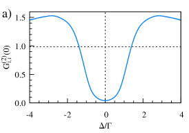
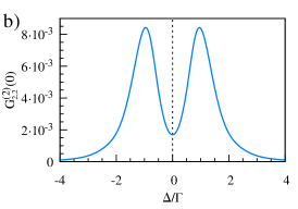
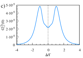
Figure 2: The second-order correlation functions of the probe beams in the output normalized to the intensity of the input pulse. The correlation functions are calculated using Eq. (47), where the wave functions are obtained by solving Eqs. (41) (46). The parameters used in numerical solution are: optical density $\alpha=30$, Rydberg blockade radius $r_{\mathrm{b}}/L_{\mathrm{abs}}=0.4$, and ratio of non-diagonal elements of the group velocity matrix to the diagonal elements $v_{1,2}/v_{1,1}=1/2$.

As an example, let us consider a situation where the diagonal matrix elements of the group velocity matrix are equal, $v_{1,1}=v_{2,2}$ and off-diagonal elements are real-valued, giving $v_{1,2}=v_{2,1}$. This can be the case when all Rabi frequencies of the control fields are real-valued and satisfy the conditions $\Omega_{2,2}=\Omega_{1,1},\Omega_{2,1}=\Omega_{1,2}$. In this situation the group velocity matrix

$$v=\frac{L_{\mathrm{abs}}}{\Gamma}\left(\begin{array}[]{cc}\Omega_{11}^{2}+\Omega_{12}^{2}&2\Omega_{11}\Omega_{12}\\ 2\Omega_{11}\Omega_{12}&\Omega_{11}^{2}+\Omega_{12}^{2}\end{array}\right)$$ (42)

has eigenvalues

$$v_{\pm}=\frac{L_{\mathrm{abs}}}{\Gamma}(\Omega_{11}\pm\Omega_{12})^{2}\,.$$ (43)

Another possibility to have such a velocity matrix is equal absolute values of the Rabi frequencies, $\Omega_{j,l}=\Omega e^{iS_{j,l}}$, together with the phases $S_{1,1}=S_{2,2}=0$ and $S_{1,2}=S_{2,1}=S\neq 0$. The group velocity matrix then is

$$\hat{v}=\frac{2L_{\mathrm{abs}}\Omega^{2}}{\Gamma}\left(\begin{array}[]{cc}1&\cos S\\ \cos S&1\end{array}\right)$$ (44)

and has eigenvalues

$$v_{\pm}=\frac{2L_{\mathrm{abs}}\Omega^{2}}{\Gamma}(1\pm\cos S)\,.$$ (45)

For the group velocity matrix having equal diagonal and off-diagonal elements, Eq. (40) for the distances $r$ much larger than the blockade radius becomes

$$i\partial_{R}\Phi_{\mathcal{E}_{j}\mathcal{E}_{l}}=-4L_{\mathrm{abs}}\left(\frac{2\Delta}{\Gamma}-i\right)\partial_{r}^{2}\Phi_{\mathcal{E}_{j}\mathcal{E}_{l}}+i\frac{v_{1,2}}{v_{1,1}}\sum_{m}\partial_{r}(\Phi_{\mathcal{E}_{j}\mathcal{E}_{m}}-\Phi_{\mathcal{E}_{m}\mathcal{E}_{l}})\,.$$ (46)

We will investigate the situation when only the first probe beam with the amplitude $a$ is incident on the atom cloud. Due to the non-diagonal matrix elements of the group velocity matrix and the presence of the atom-atom interaction $V$, outside of the atomic medium not only the first probe beam but also the second beam will be present. Since there are two probe beams, one can consider four second-order correlation functions that describe correlations between the light from the same beam as well as correlations between different beams. We will use the second-order correlation functions normalized to the intensity of the incident probe beam,

$$G_{j,l}^{(2)}(0)=\frac{1}{a^{4}}|\Phi_{\mathcal{E}_{j}\mathcal{E}_{l}}(R=L,r=0)|^{2}\,.$$ (47)

Note, that the second-order correlation functions $G_{j,l}^{(2)}$ do not depend on the amplitude of the incident beam $a$, because $\Phi_{\mathcal{E}_{j}\mathcal{E}_{l}}$ are proportional to $a^{2}$. The situation when the first probe beam is incident on the atom cloud corresponds to the boundary conditions for two-photon wave functions $\Phi_{\mathcal{E}_{1}\mathcal{E}_{1}}(z=0,z^{\prime})=\Phi_{\mathcal{E}_{1}\mathcal{E}_{1}}(z,z^{\prime}=0)=a^{2}$ and $\Phi_{\mathcal{E}_{j}\mathcal{E}_{l}}(z=0,z^{\prime})=\Phi_{\mathcal{E}_{j}\mathcal{E}_{l}}(z,z^{\prime}=0)=0$ when $j\neq 1$, $l\neq 1$. To simplify the solution we make an approximation by assuming that the boundary conditions are $\Phi_{\mathcal{E}_{1}\mathcal{E}_{1}}(R=0,r)=\Phi_{\mathcal{E}_{1}\mathcal{E}_{1}}(R,r=\pm\alpha)=a^{2}$ and $\Phi_{\mathcal{E}_{j}\mathcal{E}_{l}}(R=0,r)=\Phi_{\mathcal{E}_{j}\mathcal{E}_{l}}(R,r=\pm\alpha)=0$ when $j\neq 1$, $l\neq 1$ Firstenberg et al. (2013). In addition, we approximate the atom-atom interaction potential $V(r)$ as having a large value when $|r|<\bar{r}_{\mathrm{B}}$ and zero when $|r|>\bar{r}_{\mathrm{B}}$, where

$$\bar{r}_{\mathrm{B}}=r_{\mathrm{b}}\left(\left(\frac{2\Delta}{\Gamma}\right)^{2}+1\right)^{\frac{1}{12}}$$ (48)

is the blockade radius increased due to the presence of nonzero one-photon detuning $\Delta$. Thus the propagation equation for two-photon wave functions is given by Eq. (41) for $|r|<\bar{r}_{\mathrm{B}}$ and by Eq. (46) for $|r|>\bar{r}_{\mathrm{B}}$.

For numerical solution we take the optical depth $\alpha=30$, the ratio of the blockade radius to the absorption length $r_{\mathrm{b}}/L_{\mathrm{abs}}=0.4$ and the ratio of non-diagonal elements of the group velocity matrix to the diagonal elements $v_{1,2}/v_{1,1}=1/2$. The resulting dependence of second-order correlation functions $G_{j,l}^{(2)}(0)$ on the one-photon detuning $\Delta$, obtained by solving Eqs. (41), (46), is shown in Fig. 2. As one can see in Fig. 2a, the second-order correlation function $G_{1,1}^{(2)}(0)$ is much smaller than $1$ when one-photon detuning $|\Delta|$ is smaller that the decay rate $\Gamma$, indicating the anti-bunching of photons which arises due to the destruction of the EIT because of the Rydberg blockade. On the other hand, for large values of the one-photon detuning the second-order correlation function $G_{1,1}^{(2)}(0)$ is larger than $1$ and the photons are bunched. This bunching is a result of an effective attractive interaction between the photons Firstenberg et al. (2013, 2016). The main difference of the double-tripod scheme from the simple ladder scheme lies in the creation of the second probe beam, which is indicated by nonzero second-order correlation functions $G_{2,2}^{(2)}(0)$ and $G_{1,2}^{(2)}(0)$, shown in Figs. 2b and 2c. Although transfer of the photons from the first to the second probe beams is possible in a double-tripod setup without atom-atom interactions, to do so a nonzero two-photon detuning is needed Ruseckas et al. (2013); Lee et al. (2014). Here we considered the situation where two-photon detuning is zero and the envelope of the input probe field is constant most of the time. Therefore the appearance of the second probe beam is caused by the interactions between Rydberg atoms. As can be seen in Fig. 2b, there is an optimal value of the one-photon detuning $|\Delta|$, where the intensity of the created second probe beam is the largest. This is caused by an interplay of two effects: for small one-photon detuning $|\Delta|<\Gamma$ absorption of photons takes places due to the Rydberg blockade, whereas the efficiency of the transfer of photons from the first to the second probe beams decreases with increasing $|\Delta|$.

V Opposite signs of one-photon detunings

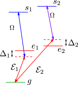
Figure 3: Double ladder atom-light coupling scheme involving the ground level $g$, the Rydberg levels $s_{1}$ and $s_{2}$, and the intermediate excited levels $e_{1}$ and $e_{2}$. Two weak probe beams with the amplitudes $\mathcal{E}_{j}$ connect the ground level $g$ to the intermediate levels $e_{j}$. Two strong control beam with the Rabi frequencies $\Omega$ connect the intermediate levels $e_{j}$ to the Rydberg levels $s_{j}$.

In the case when one-photon detunings $\Delta_{1}$ and $\Delta_{2}$ are different, numerical solution of Eqs. (28)–(30) shows that the approximation made in deriving Eq. (36) is no longer valid. Thus one cannot obtain a single approximate equation, similar to Eq. (37) describing the propagation of probe fields in the case of different one-photon detunings. To investigate the consequence of different detunings in this Section we will consider a simpler double ladder atom-light coupling scheme, shown in Fig. 3. This scheme is a particular case of the double tripod scheme with control fields $\Omega_{12}$ and $\Omega_{21}$ equal to zero. A consequence of this simplification is that the conversion of the photons between the different probe fields does not occur. In addition we will take the Rabi frequencies of the two remaining control fields to be equal: $\Omega_{11}=\Omega_{22}\equiv\Omega$. The group velocity matrix (9) for this situation becomes diagonal, with the diagonal elements equal to $v=c|\Omega|^{2}/g^{2}$.

For the double ladder scheme, the expression (30) for the wave function of two Rydberg excitations simplifies to

$$\Phi_{j,l}^{ss}=\frac{1}{2}\frac{\tilde{\Delta}_{j}^{-1}\Phi_{j,l}^{\mathcal{E}s}+\tilde{\Delta}_{l}^{-1}\Phi_{j,l}^{s\mathcal{E}}}{\tilde{V}(z^{\prime}-z)-\frac{1}{2}(\tilde{\Delta}_{j}^{-1}+\tilde{\Delta}_{l}^{-1})}\,,$$ (49)

where

$$\tilde{V}(r)=\frac{1}{|\Omega|^{2}}V(r)\,.$$ (50)

Inserting Eq. (49) into Eqs. (28)–(29) we obtain a closed pair of equations

$$c\partial_{z}\Phi_{j,l}^{\mathcal{E}s} =\frac{i}{2}g^{2}\tilde{\Delta}_{j}^{-1}\frac{\tilde{V}(r)\Phi_{j,l}^{\mathcal{E}s}+\frac{1}{2}\tilde{\Delta}_{l}^{-1}(\Phi_{j,l}^{s\mathcal{E}}-\Phi_{j,l}^{\mathcal{E}s})}{\tilde{V}(r)-\frac{1}{2}(\tilde{\Delta}_{j}^{-1}+\tilde{\Delta}_{l}^{-1})}\,,$$ (51)

$$c\partial_{z^{\prime}}\Phi_{j,l}^{s\mathcal{E}} =\frac{i}{2}g^{2}\tilde{\Delta}_{l}^{-1}\frac{\tilde{V}(r)\Phi_{j,l}^{s\mathcal{E}}+\frac{1}{2}\tilde{\Delta}_{j}^{-1}(\Phi_{j,l}^{\mathcal{E}s}-\Phi_{j,l}^{s\mathcal{E}})}{\tilde{V}(r)-\frac{1}{2}(\tilde{\Delta}_{j}^{-1}+\tilde{\Delta}_{l}^{-1})}\,.$$ (52)

The two-photon wave function $\Phi_{\mathcal{E}_{j}\mathcal{E}_{l}}$ can be calculated from the solutions of Eqs. (51), (52) using Eq. (27).

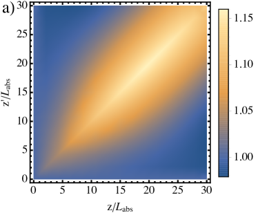
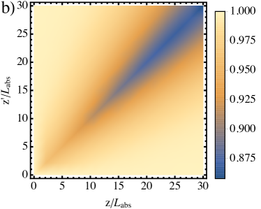
Figure 4: Square of the absolute value of the two-photon wave function a) $|\Phi_{\mathcal{E}_{1}\mathcal{E}_{1}}(z,z^{\prime})|^{2}$ and b) $|\Phi_{\mathcal{E}_{1}\mathcal{E}_{2}}(z,z^{\prime})|^{2}$, when one-photon detunings have opposite signs. The wave functions are calculated using Eqs. (51), (52) and (23). The parameters used in numerical solution are: optical density $\alpha=30$, Rydberg blockade radius $r_{\mathrm{b}}/L_{\mathrm{abs}}=0.4$, one-photon detunings $\Delta_{1}/\Gamma=-\Delta_{2}/\Gamma=2.5$.

Let us consider the situation when the one-photon detunings have opposite signs, $\Delta_{2}=-\Delta_{1}$, and both the first and second probe beams with the equal amplitudes are incident on the atom cloud. According to approximate Eqs. (51), (52), the two-photon wave function when both photons are from the same probe beam ($j=l$) behaves similarly as in an single ladder atom-light coupling scheme. This can be seen in Fig. 4a, where the two-photon wave function has amplitude larger than $1$ along the diagonal line $z=z^{\prime}$, indicating the photon bunching occuring when one-photon detuning is large, $|\Delta|>\Gamma$. More interesting is the behavior of the two-photon wave function when the photons are from different probe beams. Dependence of the square of the absolute value of the two-photon wave function $\Phi_{\mathcal{E}_{1}\mathcal{E}_{2}}(z,z^{\prime})$ on the positions $z$ and $z^{\prime}$, obtained by numerically solving Eqs. (51), (52) and (23), is shown in Fig. 4b. We assumed that both beams have equal intensities, which corresponds to the boundary conditions $\Phi_{\mathcal{E}_{1}\mathcal{E}_{2}}(0,z^{\prime})=\Phi_{\mathcal{E}_{1}\mathcal{E}_{2}}(z,0)=1$ and $\Phi_{1,2}^{\mathcal{E}s}(0,z^{\prime})=\Phi_{1,2}^{s\mathcal{E}}(z,0)=-1$. The sign “-” in the latter boundary conditions represents the fact that for a single photon inside the medium the conditions for EIT hold and the dark-state polariton forms. For numerical solution we take the atom-atom interaction potential $V(r)=C_{6}/r_{\mathrm{b}}^{6}$, optical depth $\alpha=30$, the ratio of the blockade radius to the absorption length $r_{\mathrm{b}}/L_{\mathrm{abs}}=0.4$ and the one-photon detunings $\Delta_{1}=-\Delta_{2}=2.5\Gamma$.

As one can see in Fig. 4b, the two-photon wave function, representing the correlation between the photons from different beams, has amplitude smaller than $1$ along the diagonal line $z=z^{\prime}$. This is in contrast to the two-photon wave function for the photons from the same beam, which has amplitude larger than $1$ along the diagonal when one-photon detuning is larger than $\Gamma$ (see Fig. 4a). However, the decrease of the probability to find the photons from different probe beams close to each other is not caused by photon absorption due to the Rydberg blockade which is prevented by a large one-photon detuning. We can interpret the resulting decrease of the second-order correlation function $G_{1,2}^{(2)}(0)$ as an effective repulsion between the photons from different probe beams. Note, that repulsive photon interaction can be realized in a single ladder system when the Rabi frequency of the control field is large, $|\Omega|>|\Delta|$ Bienias et al. (2014). In contrast to a single ladder system, in the double ladder system with the one-photon detunings of opposite signs, the repulsive interaction appears also for smaller Rabi frequencies $\Omega$.

VI Summary and outlook

In summary, we have derived an approximate closed equation (37) describing the propagation of the spinor Rydberg polaritons in a double-tripod setup with equal one-photon detunings. The equation shows that the dissipative or dispersive nonlinearities are combined with a spin-orbit coupling for the spinor polaritons in this system. As a consequence, the atom-atom interaction can cause transfer of a photon from one probe beam to the other. In case where the one-photon detunings have the opposite signs, the numerical solution of Eqs. (51), (52) and (23) shows the effective repulsion of the photons from different probe beams.

The proposed double tripod scheme can be experimentally implemented using a cold gas of ${}^{87}\mathrm{Rb}$ atoms Peyronel et al. (2012). The hyperfine ground state $|5S_{1/2},F=2,m_{F}=2\rangle$ in which the atoms are prepared, serves as the ground state $|g\rangle$ in our scheme. As an intermediate excited states $|e_{1}\rangle$ and $|e_{2}\rangle$ one can use a hyperfine excited states $|5P_{3/2},F=3,m_{F}=3\rangle$ and $|5P_{3/2},F=3,m_{F}=1\rangle$. Experimentally accessible values of the length of the atomic medium and the optical density are, respectively, $L=1\,\mathrm{mm}$ and $\alpha=30$ Chiu et al. (2014); Hsiao et al. (2014). The Rydberg blockade radius $r_{\mathrm{b}}$, depending on the principal quantum number of the Rydberg levels, can be of the order of $13\,\mathrm{\mu m}$ Peyronel et al. (2012).

In a future work, the description of the propagation of the spinor slow light in the medium with strong atom-atom interactions should be extended from the two-body description presented in this article, to a true many-body treatment of the system. Furthermore, the photon-photon interaction can be increased by placing an optical cavity around the atomic ensemble, resulting in the cavity-Rydberg polaritons Parigi et al. (2012); Ningyuan et al. (2016); Boddeda et al. (2016). Thus another direction of the research includes description of spinor Rydberg polaritons in a cavity.

Appendix A Solution of the equation (26)

In this appendix we solve the system of four equations

$$\sum_{m}\tilde{\Delta}_{m}^{-1}\left(v_{j,m}(\Phi_{m,l}^{\mathcal{E}s}+\Phi_{m,l}^{ss})+v_{l,m}(\Phi_{j,m}^{s\mathcal{E}}+\Phi_{j,m}^{ss})\right)-\frac{2c}{g^{2}}V(r)\Phi_{j,l}^{ss}=0$$

for the four unknown quantities $\Phi_{j,l}^{ss}$. Here $r=z-z^{\prime}$. To separate the solution into two parts let us introduce two new quantities $X_{j,l}$ and $Y_{j,l}$ such that

$$\Phi_{j,l}^{ss}=X_{j,l}+Y_{j,l}-\Phi_{j,l}^{\mathcal{E}s+}\,,$$ (53)

where

$$\Phi_{j,l}^{\mathcal{E}s+}=\frac{1}{2}(\Phi_{j,l}^{\mathcal{E}s}+\Phi_{j,l}^{s\mathcal{E}})$$ (54)

is the symmetric combination of the wave functions. This leads to the equation

$$\sum_{m}\tilde{\Delta}_{m}^{-1}\left(v_{j,m}(X_{m,l}+Y_{m,l}+\Phi_{m,l}^{\mathcal{E}s-})+v_{l,m}(X_{j,m}+Y_{j,m}-\Phi_{j,m}^{\mathcal{E}s-})\right)\\ -\frac{2c}{g^{2}}V(r)(X_{j,l}+Y_{j,l}-\Phi_{j,l}^{\mathcal{E}s+})=0\,,$$ (55)

where

$$\Phi_{j,l}^{\mathcal{E}s-}=\frac{1}{2}(\Phi_{j,l}^{\mathcal{E}s}-\Phi_{j,l}^{s\mathcal{E}})$$ (56)

is the antisymmetric combination. Since Eq. (53) defines only the sum of the quantities $X_{j,l}$ and $Y_{j,l}$, we have a freedom to impose an additional condition on those quantities. We require for the quantities $X_{j,l}$ to obey the equation

$$\sum_{m}\tilde{\Delta}_{m}^{-1}\left(v_{j,m}(X_{m,l}+\Phi_{m,l}^{\mathcal{E}s-})+v_{l,m}(X_{j,m}-\Phi_{j,m}^{\mathcal{E}s-})\right)-\frac{2c}{g^{2}}V(r)X_{j,l}=0$$ (57)

and for the quantities $Y_{j,l}$ to obey the equation

$$\sum_{m}\tilde{\Delta}_{m}^{-1}(v_{j,m}Y_{m,l}+v_{l,m}Y_{j,m})-\frac{2c}{g^{2}}V(r)Y_{j,l}=-\frac{2c}{g^{2}}V(r)\Phi_{j,l}^{\mathcal{E}s+}$$ (58)

The solution of Eq. (57) has a short analytical expression

$$X_{j,l}=\frac{1}{\tilde{\Delta}_{1}^{-1}v_{1,1}+\tilde{\Delta}_{2}^{-1}v_{2,2}-\frac{2c}{g^{2}}V(r)}\sum_{m}\tilde{\Delta}_{m}^{-1}(v_{l,m}\Phi_{j,m}^{\mathcal{E}s-}-v_{j,m}\Phi_{m,l}^{\mathcal{E}s-})\,.$$ (59)

The analytical expression for the solution of Eq. (58) is complicated. Since Eq. (58) is linear, the general form of the solution can be written as a linear combination of the terms on the right hand side of Eq. (58):

$$Y_{j,l}=-\frac{\frac{2c}{g^{2}}V(r)}{\tilde{\Delta}_{1}^{-1}v_{1,1}+\tilde{\Delta}_{2}^{-1}v_{2,2}-\frac{2c}{g^{2}}V(r)}\sum_{m,n}A_{j,l;m,n}\Phi_{m,n}^{\mathcal{E}s+}\,,$$ (60)

where the coefficients $A_{j,l;m,n}$ can be obtained from the solution of Eq. (58). In the limit of large interaction, $V(r)\gg|\Omega_{j,l}|^{2}/|\tilde{\Delta}_{j}|$ , one can drop the terms in Eq. (58) that are not proportional to $V(r)$ and obtain the solution $Y_{j,l}\approx\Phi_{j,l}^{\mathcal{E}s+}$. Thus in this limit the coefficients reduce to $A_{j,l;m,n}\approx\delta_{j,m}\delta_{l,n}$.

References

- Saffman et al. (2010) M. Saffman, T. G. Walker, and K. Mølmer, Rev. Mod. Phys. 82, 2313 (2010).
- Bohlouli-Zanjani et al. (2007) P. Bohlouli-Zanjani, J. A. Petrus, and J. D. D. Martin, Phys. Rev. Lett. 98, 203005 (2007).
- Béguin et al. (2013) L. Béguin, A. Vernier, R. Chicireanu, T. Lahaye, and A. Browaeys, Phys. Rev. Lett. 110, 263201 (2013).
- Tong et al. (2004) D. Tong, S. M. Farooqi, J. Stanojevic, S. Krishnan, Y. P. Zhang, R. Côté, E. E. Eyler, and P. L. Gould, Phys. Rev. Lett. 93, 063001 (2004).
- Singer et al. (2004) K. Singer, M. Reetz-Lamour, T. Amthor, L. G. Marcassa, and M. Weidemüller, Phys. Rev. Lett. 93, 163001 (2004).
- Heidemann et al. (2007) R. Heidemann, U. Raitzsch, V. Bendkowsky, B. Butscher, R. Löw, L. Santos, and T. Pfau, Phys. Rev. Lett. 99, 163601 (2007).
- Jaksch et al. (2000) D. Jaksch, J. I. Cirac, P. Zoller, S. L. Rolston, R. Côté, and M. D. Lukin, Phys. Rev. Lett. 85, 2208 (2000).
- Lukin et al. (2001) M. D. Lukin, M. Fleischhauer, R. Cote, L. M. Duan, D. Jaksch, J. I. Cirac, and P. Zoller, Phys. Rev. Lett. 87, 037901 (2001).
- Gaëtan et al. (2009) A. Gaëtan, Y. Miroshnychenko, T. Wilk, A. Chotia, M. Viteau, D. Comparat, P. Pillet, A. Browaeys, and P. Grangier, Nat. Phys. 5, 115 (2009).
- Urban et al. (2009) E. Urban, T. A. Johnson, T. Henage, L. Isenhower, D. D. Yavuz, T. G. Walker, and M. Saffman, Nat. Phys. 5, 110 (2009).
- Isenhower et al. (2010) L. Isenhower, E. Urban, X. L. Zhang, A. T. Gill, T. Henage, T. A. Johnson, T. G. Walker, and M. Saffman, Phys. Rev. Lett. 104, 010503 (2010).
- Cinti et al. (2010) F. Cinti, P. Jain, M. Boninsegni, A. Micheli, P. Zoller, and G. Pupillo, Phys. Rev. Lett. 105, 135301 (2010).
- Pohl et al. (2010) T. Pohl, E. Demler, and M. D. Lukin, Phys. Rev. Lett. 104, 043002 (2010).
- Pupillo et al. (2010) G. Pupillo, A. Micheli, M. Boninsegni, I. Lesanovsky, and P. Zoller, Phys. Rev. Lett. 104, 223002 (2010).
- Viteau et al. (2011) M. Viteau, M. G. Bason, J. Radogostowicz, N. Malossi, D. Ciampini, O. Morsch, and E. Arimondo, Phys. Rev. Lett. 107, 060402 (2011).
- Carr et al. (2013) C. Carr, R. Ritter, C. G. Wade, C. S. Adams, and K. J. Weatherill, Phys. Rev. Lett. 111, 113901 (2013).
- Schauss et al. (2015) P. Schauss, J. Zeiher, T. Fukuhara, S. Hild, M. Cheneau, T. Macrì, T. Pohl, I. Bloch, and C. Gross, Science 347, 1455 (2015).
- Petrosyan et al. (2011) D. Petrosyan, J. Otterbach, and M. Fleischhauer, Phys. Rev. Lett. 107, 213601 (2011).
- Gorshkov et al. (2011) A. V. Gorshkov, J. Otterbach, M. Fleischhauer, T. Pohl, and M. D. Lukin, Phys. Rev. Lett. 107, 133602 (2011).
- Dudin and Kuzmich (2012) Y. O. Dudin and A. Kuzmich, Science 336, 887 (2012).
- Dudin et al. (2012) Y. O. Dudin, L. Li, F. Bariani, and A. Kuzmich, Nat. Phys. 8, 790 (2012).
- Peyronel et al. (2012) T. Peyronel, O. Firstenberg, Q.-Y. Liang, S. Hofferberth, A. V. Gorshkov, T. Pohl, M. D. Lukin, and V. Vuletić, Nature 488, 57 (2012).
- Firstenberg et al. (2013) O. Firstenberg, T. Peyronel, Q.-Y. Liang, A. V. Gorshkov, M. D. Lukin, and V. Vuletić, Nature 502, 71 (2013).
- Li et al. (2013) L. Li, Y. O. Dudin, and A. Kuzmich, Nature 498, 466 (2013).
- Chang et al. (2014) D. Chang, V. Vuletíc, and M. D. Lukin, Nature Photonics 8, 685 (2014).
- Bienias et al. (2014) P. Bienias, S. Choi, O. Firstenberg, M. F. Maghrebi, M. Gullans, M. D. Lukin, A. V. Gorshkov, and H. P. Büchler, Phys. Rev. A 90, 053804 (2014).
- Firstenberg et al. (2016) O. Firstenberg, C. S. Adams, and S. Hofferberth, J. Phys. B: At. Mol. Opt. Phys. 49, 152003 (2016).
- Unanyan et al. (2010) R. G. Unanyan, J. Otterbach, M. Fleischhauer, J. Ruseckas, V. Kudriašov, and G. Juzeliūnas, Phys. Rev. Lett. 105, 173603 (2010).
- Ruseckas et al. (2011) J. Ruseckas, V. Kudriašov, G. Juzeliūnas, R. G. Unanyan, J. Otterbach, and M. Fleischhauer, Phys. Rev. A 83, 063811 (2011).
- Ruseckas et al. (2013) J. Ruseckas, V. Kudriašov, I. A. Yu, and G. Juzeliūnas, Phys. Rev. A 87, 053840 (2013).
- Lee et al. (2014) M.-J. Lee, J. Ruseckas, C.-Y. Lee, V. Kudriašov, K.-F. Chang, H.-W. Cho, G. Juzeliūnas, and I. A. Yu, Nat. Commun. 5, 5542 (2014).
- Bérard and Mohrbach (2004) A. Bérard and H. Mohrbach, Phys. Rev. D 69, 127701 (2004).
- Bliokh and Bliokh (2004a) K. Y. Bliokh and Y. P. Bliokh, Phys. Lett. A 333, 181 (2004a).
- Bliokh and Bliokh (2004b) K. Y. Bliokh and Y. P. Bliokh, Phys. Rev. E 70, 026605 (2004b).
- Onoda et al. (2004) M. Onoda, S. Murakami, and N. Nagaosa, Phys. Rev. Lett. 93, 083901 (2004).
- Bérard and Mohrbach (2006) A. Bérard and H. Mohrbach, Phys. Lett. A 352, 190 (2006).
- Duval et al. (2006) C. Duval, Z. Horváth, and P. A. Horváthy, Phys. Rev. D 74, 021701 (2006).
- Duval et al. (2007) C. Duval, Z. Horváth, and P. A. Horváthy, J. Geom. Phys. 57, 925 (2007).
- Fleischhauer and Lukin (2002) M. Fleischhauer and M. D. Lukin, Phys. Rev. A 65, 022314 (2002).
- Gorshkov et al. (2007) A. V. Gorshkov, A. André, M. D. Lukin, and A. S. Sørensen, Phys. Rev. A 76, 033805 (2007).
- Li et al. (2014) W. Li, D. Viscor, S. Hofferberth, and I. Lesanovsky, Phys. Rev. Lett. 112, 243601 (2014).
- Gorniaczyk et al. (2016) H. Gorniaczyk, C. Tresp, P. Bienias, A. Paris-Mandoki, W. Li, I. Mirgorodskiy, H. Büchler, I. Lesanovsky, and S. Hofferberth, Nat. Commun. 7, 12480 (2016).
- van Bijnen (2013) R. van Bijnen, Quantum engineering with ultracold atoms, Ph.D. thesis, Eindhoven University of Technology (2013).
- Scully and Zubairy (1997) M. O. Scully and M. S. Zubairy, Quantum Optics (Cambridge Univesity Press, Cambridge, 1997).
- Gorshkov et al. (2013) A. V. Gorshkov, R. Nath, and T. Pohl, Phys. Rev.Lett. 110, 153601 (2013).
- Hafezi et al. (2012) M. Hafezi, D. E. Chang, V. Gritsev, E. Demler, and M. D. Lukin, Phys. Rev. A 85, 013822 (2012).
- Chiu et al. (2014) C.-K. Chiu, Y.-H. Chen, Y.-C. Chen, I. A. Yu, Y.-C. Chen, and Y.-F. Chen, Phys. Rev. A 89, 023839 (2014).
- Hsiao et al. (2014) Y.-F. Hsiao, H.-S. Chen, P.-J. Tsai, and Y.-C. Chen, Phys. Rev. A 90, 055401 (2014).
- Parigi et al. (2012) V. Parigi, E. Bimbard, J. Stanojevic, A. J. Hilliard, F. Nogrette, R. Tualle-Brouri, A. Ourjoumtsev, and P. Grangier, Phys. Rev. Lett. 109, 233602 (2012).
- Ningyuan et al. (2016) J. Ningyuan, A. Georgakopoulos, A. Ryou, N. Schine, A. Sommer, and J. Simon, Phys. Rev. A 93, 041802 (2016).
- Boddeda et al. (2016) R. Boddeda, I. Usmani, E. Bimbard, A. Grankin, A. Ourjoumtsev, E. Brion, and P. Grangier, J. Phys. B: At. Mol. Opt. Phys. 49, 084005 (2016).