A Missing Information Loss for implicit feedback datasets

Abstract.

Latent factor models for Recommender Systems with implicit feedback typically treat unobserved user-item interactions (i.e. missing information) as negative feedback. This is frequently done either through negative sampling (point–wise loss) or with a ranking loss function (pair– or list–wise estimation). Since a zero preference recommendation is a valid solution for most common objective functions, regarding unknown values as actual zeros results in users having a zero preference recommendation for most of the available items.

In this paper we propose a novel objective function, the Missing Information Loss (MIL), that explicitly forbids treating unobserved user-item interactions as positive or negative feedback. We apply this loss to both traditional Matrix Factorization and user–based Denoising Autoencoder, and compare it with other established objective functions such as cross–entropy (both point– and pair–wise) or the recently proposed multinomial log-likelihood. MIL achieves competitive performance in ranking–aware metrics when applied to three datasets. Furthermore, we show that such a relevance in the recommendation is obtained while displaying popular items less frequently (up to a $20\%$ decrease with respect to the best competing method). This debiasing from the recommendation of popular items favours the appearance of infrequent items (up to a $50\%$ increase of long–tail recommendations), a valuable feature for Recommender Systems with a large catalogue of products.

1. Introduction

Nowadays, users are faced with such a large volume of products and information to the extent that filtering has become a necessity. Furthermore, not every user has the same preferences, and therefore a standard selection cannot be performed. Both problems can be tackled with Recommender Systems (RS), that provide users with a personalized list of items. Moreover, for organizations with vast inventories, it is of great interest to recommend infrequent products, i.e. items queuing in the long tail of the catalogue of items (Anderson:2006:long_tail, ). Nevertheless, most RS algorithms tend to over-recommend popular items, precisely because their metric performance generally decreases when recommending less frequent items (Steck:2011:IPR, ).

An increasingly adopted approach to RS is collaborative filtering (CF) for implicit feedback datasets (HuKoren:2008:CF_implicit, ; Pan:2008:OCCF, ). This technique makes predictions about the interests of a user by gathering preferences in the form of purchases, clicks, logs, etc. from many other users. These preferences are influenced by non-obvious factors that depend on the domain. The goal of model based CF approaches such as matrix factorization is to infer the latent factor model underlying the data.

Making predictions about user preferences in RS based on implicit feedback data is not an easy task, not only because of the lack of information about unobserved user-item interactions, but also due to the subsequent high sparsity of the rating matrix. In order to deal with this issue of missing information, several approaches can be considered. A naive strategy for one–class collaborative filtering consists of considering all unobserved items either as negative examples (All Missing As Negative) or simply to ignore them (All Missing As Unknown) (Pan:2008:OCCF, ). However, these two extreme methodologies may involve either biased recommendations (as some of the missing data might be relevant to the user) or trivial solutions caused by predicting all missing values as positive examples. More advanced approaches entail the use of different weighting schemes in the error terms to balance observed and unobserved items (HuKoren:2008:CF_implicit, ; Pan:2008:OCCF, ; Steck:2010:MissingNotAtRandom, ). In order to alleviate the computational burden of considering every single item during the training process (which does not scale linearly as the item catalogue grows), several negative sampling techniques have been proposed, see e.g. (Pan:2008:OCCF, ).

It should be noted that all these approaches cast missing entries as zeros, i.e. treat unobserved user-item interactions as negative feedback. Since the loss functions considered in those works are designed to push items with negative feedback towards a zero recommendation, in practice a zero preference will be inferred for most of the missing entries.

In addition to the one-class collaborative filtering setting, the RS problem can be viewed as a multi-class classification problem, where the recommendation problem is cast as the calculation of the probability of a user belonging to each item class. Indeed, the multinomial distribution has been recently applied to different Autoencoder (AE) architectures (liang:2018:VAE, ). In contrast to the above-mentioned objective functions, the log-likelihood of the multinomial distribution does not explicitly penalize missing entries so as to force them to have a zero probability of being recommended. However, the normalization condition of the probability distribution, together with the large item catalogues used in RS (typically $>10$k items), make it unlikely that non-seen items have a probability of being recommended other than zero.

In this paper we propose to tackle the problem of missing information by using a novel objective function that specifically forbids missing user–item interactions to have a preference prediction of $1$ (since they are not positive feedback) or $0$ (to distinguish them from negative feedback). We name this cost function the Missing Information Loss (MIL). We apply MIL to both Matrix Factorization (ML) and Denoising AE (DAE) (Vincent:2008:ECRF-AE, ), as the later has been shown to be a generalization of traditional MF models (Wu:2016:CDAE-topN, ). We compare the results with DAEs optimized with cross-entropy loss (in both point and pair–wise learning schemes) (Wu:2016:CDAE-topN, ) and the multinomial loss (liang:2018:VAE, ); as well as MF models (HuKoren:2008:CF_implicit, ) trained with square and cross-entropy loss.

Our contributions can be summarized as follows:

• We propose a new objective function (MIL) for modeling missing information in implicit feedback datasets. It explicitly forbids either a $1$ or $0$ prediction for the preference of unobserved user–item interactions, thus leaving the ranking process almost entirely to the low-rank process underlying all forms of matrix factorization.

• We show that the MIL function achieves state-of-the-art metric performance when applied to MF and DAE architectures, similar to the best performing, well established, objective functions.

• Furthermore, we demonstrate that the observed competitive performance (in terms of relevance) occur while recommending popular items less frequently, which favours the appearance of medium and long–tail items in the ranked list of recommendations.

The rest of the paper is organized as follows. In section 2 we review some of the objective functions that are commonly used in RS literature, and introduce the MIL function. Next, we briefly revisit the DAE and MF architectures. After that, in section 3, we describe the experimental methodology: datasets, metrics for evaluation, the implementation details of the proposed solution, and the baseline models used for comparison. Next, section 4 shows the experimental results in terms of ranking metrics, as well as the observed distribution of recommendations. Finally, we draw some conclusions in section 5 and indicate future lines of research.

2. Model

Let $\mathcal{U}$ be the set of users and $|\mathcal{U}|$ the total number of users. Let $\mathcal{I}$ be the set of available items and $\mathcal{I}_{u}$ the set adopted by user $u$. The number of total items is denoted by $|\mathcal{I}|$, and those adopted by a user $|\mathcal{I}_{u}|$. Our goal is to predict the preference of a user for all the available items given its history of binary preferences $p_{ui}\mid i\in\mathcal{I}_{u}$, i.e. calculate $\hat{p}_{ui}~{}\forall i\in\mathcal{I}$. Next, we review some familiar objective functions, and introduce our Missing Information Loss (MIL) function. Then, we revisit the user–based Denoising Autoencoder (DAE) (Kramer:1991:NLPCA, ; Vincent:2008:ECRF-AE, ) and specify its usage for RS (Sedhain:2015:Autorec, ; Wu:2016:CDAE-topN, ).

2.1. Objective functions for Recommender Systems

Learning to assign user preferences for items depends to a great extent on how the objective function–i.e., the function we intend to optimize–is set. In this subsection we review the most relevant objective functions considered in the literature for the task of recommendation, with a special focus on the missing information issue.

Regarding the square loss, a confidence scale factor for balancing the observed and unobserved items is introduced in (HuKoren:2008:CF_implicit, ). This factor can be defined as $C(p_{ui}):=ap_{ui}$, with $a>1$ a hyper-parameter for ensuring a correct balance. Using such confidence scale factor, the square loss is cast as

(1) $$l(p_{ui},\hat{p}_{ui})=\frac{C(p_{ui})+1}{2}\left(p_{ui}-\hat{p}_{ui}\right)^{2}.$$

Similarly, the cross-entropy objective function can be generalized to account for the unbalance of classes,

(2) $$l\left(p_{ui},\hat{p}_{ui}\right)=-C\left(p_{ui}\right)\log\left(\hat{p}_{ui}\right)-\left(1-p_{ui}\right)\log\left(1-\hat{p}_{ui}\right).$$

In both cases, the total loss is averaged across all users,

(3) $$\mathcal{L}_{\rm point}=\frac{1}{|\mathcal{U}|}\sum_{u\in\mathcal{U}}\sum_{i\in\mathcal{I}}l\left(p_{ui},\hat{p}_{ui}\right).$$

Please note that casting unobserved user-item interactions as $p_{ui}=0$ in equations (1) and (2), induces many zero recommendations, i.e. $\hat{p}_{ui}=0$. With all certainty, the limited capacity of the model (the low–rank process) avoids setting all unobserved items with a zero preference prediction.

Due to the large item catalogues typically involved in RS, negative sampling techniques are used to solve the positive/negative class unbalance problem (Pan:2008:OCCF, ; Wu:2016:CDAE-topN, ). For this, a target set $\mathcal{T}_{u}$ is built by joining the observed item set $\mathcal{I}_{u}$ and items sampled from $\mathcal{\tilde{I}}_{u}:=\mathcal{I}\setminus\mathcal{I}_{u}$. The number of items sampled from $\mathcal{\tilde{I}}_{u}$ is a hyper-parameter to be tuned, while $C(p_{ui})$ in equations (1) and (2) is set to $1$ for all preferences. The loss is then computed as

(4) $$\mathcal{L}_{\rm point}=\frac{1}{|\mathcal{U}|}\sum_{u\in\mathcal{U}}\sum_{i\in\mathcal{T}_{u}}l\left(p_{ui},\hat{p}_{ui}\right).$$

The above objective functions are examples of point-wise learning, where the loss is calculated by taking the information of only one item at a time. Rendle et al. (Rendle:2009:BPR, ) introduced pair-wise learning, which confronts a pair of items (positive and unobserved) to compute the final loss. Because of this, a new set $\mathcal{P}_{u}$ consisting of pairs of seen (positive feedback) and unseen items (assumed negative feedback) is created. The total pair-wise loss is then defined as (Wu:2016:CDAE-topN, )

(5) $$\mathcal{L}_{\rm pair}=\frac{1}{|\mathcal{U}|}\sum_{u\in\mathcal{U}}\sum_{i,j\in\mathcal{P}_{u}}l\left(p_{uij},\hat{p}_{uij}\right).$$

Here, $p_{uij}:=p_{ui}-p_{uj}=1,\forall(i,j)\in\mathcal{P}_{u}$ and $\hat{p}_{uij}:=\hat{p}_{ui}-\hat{p}_{uj}$.

For both point and pair–wise learning schemes, the objective functions defined in equations (1) and (2) admit as a valid solution a predicted zero preference when the input preference is zero, i.e. $\hat{p}_{ui}=0$ if $p_{ui}=0$. However, it should be noted that in implicit feedback datasets there are no actual zero preferences, but rather missing information. Thus, by using any of the losses described above the solution will inevitably assign zero preferences to most of the unobserved user-item pairs. This fact affects the way in which items are recommended, as discussed in section 4.

On the other hand, a model based on the multinomial distribution has been recently applied to AEs by Liang et al. (liang:2018:VAE, ). The log-likelihood for a user $u$ in this setting can be written as

(6) $$-\sum_{i}p_{ui}\log\pi_{i}\left(\hat{p}_{ui}\right)$$

where $\pi_{i}\left(\hat{p}_{ui}\right)$ is the probability distribution of the predictions. Note that in contrast to the square and cross–entropy losses, this objective function does not explicitly penalize missing values, since $p_{ui}=0$ for unobserved user–item interactions. Instead, the normalization condition of the probability distribution ($\sum_{i}\pi_{i}\left(\hat{p}_{ui}\right)=1$), together with the low–rank process, helps to assign non-zero preferences to the unobserved items. However, the large item catalogues used in RS (typically $>10$k) make it unlikely that non-seen items have a probability different from zero. Furthermore, the normalization condition on the probabilities prevent this modeling from scaling up.

In order to mitigate all the problems mentioned within this subsection, we propose a novel objective function, the Missing Information Loss (MIL), that explicitly forbids treating missing information as positive or negative feedback. For this reason, we propose the functional form

(7) $$l(p_{ui},\hat{p}_{ui}) = \frac{1}{2}p_{ui}(1+p_{ui})(1-\hat{p}_{ui})^{\gamma_{+}}+$$

$$\frac{1}{2}(1+p_{ui})(1-p_{ui})A_{\rm MI}(\hat{p}_{ui}-0.5)^{2\gamma_{\rm MI}}.$$

Here, the first and second term evaluate the contribution of the observed and unobserved user-item pairs into the final loss. In particular, the first term estimates preferences for positive items as a power law with parameter $\gamma_{+}$. Indeed, for $p_{ui}=1$ equation (7) reduces to

$$l(p_{ui}=1,\hat{p}_{ui})=(1-\hat{p}_{ui})^{\gamma_{+}}.$$

On the other hand, the last term in (7) explicitly forbids predicted 0 and 1 preferences for missing entries, acting as a barrier for the optimization process. As a matter of fact, for $p_{ui}=0$ equation (7) is cast as

$$l(p_{ui}=0,\hat{p}_{ui})=A_{\rm MI}(\hat{p}_{ui}-0.5)^{2\gamma_{\rm MI}}.$$

The constants $A_{\rm MI}$ and $\gamma_{\rm MI}$ are hyper-parameters to be fine-tuned. In this paper we explore the pairs $\left(A_{\rm MI},\gamma_{\rm MI}\right)\in\{(5\cdot 10^{1},2)$, $(10^{3},4)$, $(2\cdot 10^{4},6)$, $(1\cdot 10^{6},10)$, $(5\cdot 10^{9},15)\}$, see Figure 1.

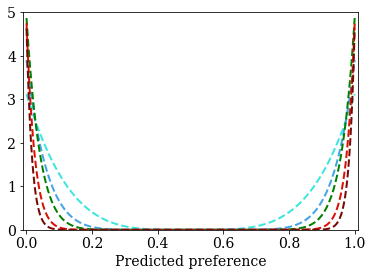
Figure 1. Different values of the hyper-parameters $\boldsymbol{A_{\rm MI}}$ and $\boldsymbol{\gamma_{\rm MI}}$ modeling the missing information term in equation (7). The exponent of each polynomial here is, from the smoothest to the sharpest curves, $\boldsymbol{2\gamma_{\rm MI}\equiv\{4,8,12,20,30\}}$.

At this point, it is worth stressing that under the MIL function all items–independently of their position into the long tail curve–can be part of the recommendation process, as their predicted preferences adopt non-zero values, $\hat{p}_{ui}\in(0,1)$. Thus, the final predicted preference will be adjusted by the collaborative filtering among users, the co-occurrence of items, and the limited capacity of the model–i.e., the overall low–rank process.

Note that the MIL function in equation (7) can be naturally extended to account for actual negative feedback, i.e $p_{ui}=-1$. Indeed, we can simply add the term

(8) $$-\frac{1}{2}p_{ui}(p_{ui}-1)\hat{p}_{ui}^{\gamma_{-}}.$$

to equation (7), which vanishes whenever $p_{ui}=0,1$. Here, $\gamma_{-}$ is an exponent controlling the family of polynomials modeling negative feedback entries. Such a term would force negative ratings to have a zero predicted preference. We will leave the analysis of datasets with actual negative feedback for future study.

Finally, for any given loss function we regularize the model with weight-decay, so that the total loss is

(9) $$\mathcal{L}=\mathcal{L}_{\rm point/pair}+\lambda\left(||{\bf W}||_{2}^{2}+||{\bf W^{\prime}}||_{2}^{2}\right).$$

Here, $\lambda$ is a hyper-parameter.

2.2. Architecture details

We represent an item $i$ is as a one-hot encoding ${\bf v}_{i}$, i.e. a $|\mathcal{I}|$-sized vector of zeros with a $1$ at position $i$. Next, we represent a user $u$ as the sum of the one-hot encoding vectors of items in $\mathcal{I}_{u}$,

(10) $${\bf v}_{u}:=\sum_{i\in\mathcal{I}_{u}}{\bf v}_{i}=\sum_{i\in\mathcal{I}}p_{ui}{\bf v}_{i},$$

where $p_{ui}$ is the preference of user $u$ for item $i$, i.e. $p_{ui}=1$ if $i\in\mathcal{I}_{u}$, $p_{ui}=0$ otherwise. The vector of preferences is therefore equal to the user vector in our setting, ${\bf p}_{u}\equiv{\bf v}_{u}$. In the general case of non binary implicit ratings $r_{ui}$ (such as purchases or play counts) the user vector will consist of the weighted sum of the one-hot encoding of their items,

(11) $${\bf v}_{u}:=\sum_{i\in\mathcal{I}_{u}}r_{ui}{\bf v}_{i}.$$

An Autoencoder (AE) (Kramer:1991:NLPCA, ) is a feedforward neural network for learning a representation of the input data. This representation is trained to produce an output that closely matches the original input. When applied to RS, the encoder typically has a much lower dimension than the input vector; hence, the learned representation has to encode input information while reducing the dimensionality of the input space. In this paper we consider a single hidden layer AE. The input vector of preferences, ${\bf p}_{u}\in\mathbb{R}^{|\mathcal{I}|}$, is projected onto a vector ${\bf h}\in\mathbb{R}^{D}$,

(12) $${\bf h}=s({\bf W}{\bf v}_{u}+{\bf b}).$$

Here ${\bf W}\in\mathbb{R}^{D\times|\mathcal{I}|}$ and ${\bf b}\in\mathbb{R}^{D}$ are learnable weight matrix and bias vectors, respectively. The activation $s(\cdot)$ is an element-wise mapping function; typical activations are the sigmoid function, the hyperbolic tangent or the Rectified Linear Unit (ReLU) (icml2010_NairH10_Relu, ).

In order to obtain the predicted preferences, the hidden layer is projected back onto the original space,

(13) $$\hat{\bf p}_{u}=s^{\prime}({\bf W}^{\prime}{\bf h}+{\bf b}^{\prime}),$$

where ${\bf W}^{\prime}\in\mathbb{R}^{|\mathcal{I}|\times D}$ and ${\bf b}^{\prime}\in\mathbb{R}^{|\mathcal{I}|}$ are weight matrix and bias vectors for the output layer, and $s^{\prime}(\cdot)$ is the activation of the decoder (which may or may not be equal to that used when encoding). The vector of predicted preferences, $\hat{\bf p}_{u}$, is then forced to minimize the objective functions defined in subsection 2.1. A variant of the AE is the Denoising Autoencoder (DAE) (Vincent:2008:ECRF-AE, ), which attempts to reconstruct a corrupted version of the input $\tilde{{\bf x}}$, i.e. ${\bf h}=s({\bf W}\tilde{{\bf x}}+{\bf b})$. This latter technique has become very popular due to its success in image recognition, and is currently applied in most AEs for RS (Wu:2016:CDAE-topN, ; liang:2018:VAE, ).

Please note that for MIL and cross-entropy losses (equations (7) and (2) respectively), output preferences must be bounded $\hat{p}_{ui}\in(0,1)$. Thus, we typically choose the sigmoid function for the activation of the decoder, $s^{\prime}=\sigma$. This is different from the also traditional approach of minimizing the logistic log-likelihood (Wu:2016:CDAE-topN, ; liang:2018:VAE, ), which already incorporates the sigmoid function into the loss, and thus allows one to apply yet another activation at the decoder (e.g. $\tanh(\sigma(\hat{p}_{ui}))$, as in (liang:2018:VAE, ), or $\sigma(\sigma(\hat{p}_{ui}))$ in (Wu:2016:CDAE-topN, )).

Matrix Factorization

As shown in (Wu:2016:CDAE-topN, ), the AE described in equations (10), (12) and (13) is a generalization of Matrix Factorization (MF) models. Indeed, MF is recovered after replacing the input user vector (10) by the one-hot vector of the user id $u$, which is a $|\mathcal{U}|$–sized vector of zeros with a 1 at the position $u$. The bi–linear MF has linear activations $s$ and $s^{\prime}$, and is typically trained with square loss and weight–decay regularization, see equations (1), (4) and (9).

However, due the the large disparity in the number of users and items, $|\mathcal{U}|\ll|\mathcal{I}|$, the norms of the weight matrices ${\bf W}\in\mathbb{R}^{D\times|\mathcal{U}|}$ and ${\bf W^{\prime}}\in\mathbb{R}^{|\mathcal{I}|\times D}$ are quite different. Thus, direct application of equation (9) will tend to over-regularized the user matrix ${\bf W}$, leaving the item one ${\bf W^{\prime}}$ under-regularized; this may lead to instabilities and potential over-fitting while training (as we have observed experimentally). This issue can be solved by re-scaling the norms of weight matrices in equation (9) as

(14) $$\mathcal{L}=\mathcal{L}_{\rm point/pair}+\frac{\lambda}{D}\left(\frac{||{\bf W}||_{2}^{2}}{|\mathcal{U}|}+\frac{||{\bf W^{\prime}}||_{2}^{2}}{|\mathcal{I}|}\right).$$

This way, both user and item embeddings are regularized with the same strength, stabilizing the training procedure. Note: in the case of an AE, there is no need to re-scale the norm of weights matrices, since both have the same number of elements, $|\mathcal{I}|\times D$.

3. Experimental protocols

3.1. Datasets

We use the MovieLens–20M and Netflix explicit feedback datasets. As both of these contain explicit ratings, we create binary preferences by keeping ratings $\geq\!4$, which we interpret as positive feedback ($p_{ui}=1$). Furthermore, we only keep users with at least 5 views. Validation and test sets are obtained randomly, selecting a $10~{}\%$ of the original dataset for each set. We denote such datasets ML20M and Netflix.

In addition, we explore models performance on the Last.fm dataset (Celma:Springer2010, ), an implicit feedback dataset consisting of tuples (user, artist, plays), that contains top artists by user. In order to make the comparison with the above datasets more straightforward, we binarize play counts and interpret them as implicit preference data. Next, we filter out artist with less than 50 distinct listening users, and user with less than 20 artists in their listening history. In the following, we name this dataset Lastfm.

Dataset	#users	#items	#pairs	#pairstest
ML20M	136,7k	20,3k	7,99M	1,0M
Netflix	463,4k	17,7k	45,5M	5,7M
Lastfm	350,2k	24,6k	12,8M	1,6M

Table 1. Statistics of the datasets after preprocessing.

The statistics of the training set after such processing, as well as the number of user-item interactions in test, are presented in Table 1.

3.2. Evaluation metrics

Given the set of adopted items in test, $\mathcal{I}_{u}^{\rm t}$, and the ranked list of predicted preferences, the relevance of a recommendation at position $k$ is given by ${\rm rel}_{ui}(k)$–${\rm rel}(k)$ from here on–, which equals $1$ if user $u$ adopted item $i$ in the test set, $0$ otherwise. In the calculation of metrics, we remove items observed in training and validation from the list of recommendations. Next, we detail the metrics used for model evaluation.

Recall

It does not account for the relative ordering of the recommendation, and we defined it as (liang:2018:VAE, )

(15) $${\rm Recall}@k=\frac{\sum_{s=1}^{k}{\rm rel}(s)}{\mathcal{N}_{u}(k)}.$$

Here, $\mathcal{N}_{u}(k)=\min\left(k,|\mathcal{I}_{u}^{\rm t}|\right)$, with $|\mathcal{I}_{u}^{\rm t}|$ the number of items adopted by user $u$ in testing. The final recall is averaged across all users in testing.

Normalized Discount Cumulative Gain

In contrast to recall metric, the Discount Cumulative Gain (DCG) performs a logarithmic discount according to the position of a recommendation, that is

(16) $${\rm DCG}@k=\sum_{s=1}^{k}\frac{{\rm rel}(s)}{\log_{2}(s+1)}.$$

This quantity can be normalized by the Ideal DCG,

(17) $${\rm IDCG}@k=\sum_{s=1}^{\mathcal{N}_{u}(k)}\frac{1}{\log_{2}(s+1)}.$$

Finally, NDCG$@k={\rm DCG}@k/{\rm IDCG}@k$, which we average across all users in the test set.

Novelty

Following reference (Vargas:2011:Novelty_diversity, ), we define a novelty-weighted DCG score as

(18) $${\rm Nov\!-\!DCG}@k=-\sum_{s=1}^{k}\frac{{\rm rel}(s)\times\ln{\nu(i)}}{\log_{2}(s+1)}.$$

Here, $\nu(i)$ is the frequency of occurrences of item $i$ normalized to the total interactions in training. The corresponding novelty-weighted IDCG would be

(19) $${\rm Nov\!-\!IDCG}@k=\sum_{s=1}^{\mathcal{N}_{u}(k)}\frac{\max_{i\in\mathcal{I}_{u}}\left(-\ln\nu(i)\right)}{\log_{2}(s+1)}.$$

In other words, the highest DCG is obtained by ranking the most novel items (among those relevant to the user) in descending order.

3.3. Implementation details

The implementation of our model is performed in TensorFlow (tensorflow2015-whitepaper, ). The model can be trained in both CPU or GPU. When GPU is enabled, the use of queues to feed the tensors greatly speeds up the training. We set the batch size to $100$, and train every DAE model for $120$k iterations, so as to ensure proper convergence. For MF models we use $180$k iterations. The number of neurons is $200$ in all DAE experiments; for MF models, since the large number of users makes them prone to overfit, we train the models with $100$ and $200$ neurons and take the best performing model. Weight matrices are initialized with random uniform values whose amplitude is computed as described by Glorot et al. (Xavier_initialization, ). For the biases we use a truncated random normal initialization with a standard deviation of $10^{-3}$. Models are trained with Adam optimizer (Kingma2014AdamAM, ) and a learning rate of $10^{-3}$.

Concerning negative sampling in point and pair–wise schemes, we fix the size of the target sets for every user (sets $\mathcal{T}_{u}$ and $\mathcal{P}_{u}$ for point and pair–wise learning, respectively, see subsection 2.1). In particular, we make such sets proportional to the median number of items adopted by users, except for the multinomial loss, where all items are utilized (Liang:2016:CoFactor, ). The proportionality factors are hyper-parameters fine–tuned with the validation set, swapping the values $\{1,\,5,\,10,\,50,\,100,\,150\}$. We find a factor of $50$ or $100$ to provide the best results.

We add noise to the input vector of the AE (Vincent:2008:ECRF-AE, ; Wu:2016:CDAE-topN, ) using drop-out (liang:2018:VAE, ). We fix the level of noise at $0.5$. Competitive performance is achieved after normalizing the AE input vector. For DAE models, we swap the $L_{2}$ regularization strength $\lambda\in[10^{-7}-10^{-4}]$, while for MF models we take the form in equation (14) with $\lambda\in[10^{0}-10^{3}]$, which provides a more stable training for MF models. In general we find that MIL models require smaller $\lambda$ factors than cross-entropy or multinomial–based models. This is expected, as the level of weight–decay regularization in equations (9) and (14) depends on the value of the loss, which is smaller for MIL models.

3.4. Baseline models

We implement the objective functions described in subsection 2.1 on a user-based DAE (Sedhain:2015:Autorec, ; Wu:2016:CDAE-topN, ) and compare the results with the MIL function. We also compare them with traditional Matrix Factorization with Weight Regularization (HuKoren:2008:CF_implicit, ). In the following, we provide details on the training of the different models.

Weight-Regularized Matrix Factorization WRMF (HuKoren:2008:CF_implicit, ) is a linear factorization model trained with square loss and weight decay. We use negative sampling with a sampling ratio of $100$ and $\lambda\sim 5-10$ (as obtained in the validation set). We call this model MF-square. In addition, we train WRMF models with MIL and point–wise cross–entropy losses, applying a sigmoid function at the output, so as to ensure $\hat{p}_{ui}\in(0,1)$. In these cases, we find that a sampling ratio of $100$ and $\lambda=50-500$ provide best results. We name these models MF-mil  and MF-CE, respectively.

Denoising Autoencoder models

Cross-entropy loss For the cross-entropy loss defined in equations (2), (4) and (5), we use linear–sigmoid and sigmoid–sigmoid activations at the encoder and decoder, respectively. We name the DAEs models with cross-entropy loss and point–wise estimation CE_Point lin-sig and CE_Point sig-sig; and those with pair–wise, CE_Pair lin-sig and CE_Pair sig-sig. In order to prevent numerical instabilities, we ensure that the output preferences are in $[\varepsilon,1-\varepsilon]$, with $\varepsilon=10^{-5}$. Regarding negative sampling, we find that the best sampling ratio is $50\times{\rm median}(\mathcal{I}_{u})$ and $100\times{\rm median}(\mathcal{I}_{u})$ for point and pair–wise estimation, respectively. Best weight-decay regularization is found to be $\lambda=2\cdot 10^{-5}$.

The closest model to these baselines is the Collaborative Denoising AE (CDAE) (Wu:2016:CDAE-topN, ), although for the sake of simplicity, in the present paper we do not include the user embedding of CDAE. Similar to CDAE, we find that pair–wise learning does not achieve competitive results at the top of the ranked list (Wu:2016:CDAE-topN, ; liang:2018:VAE, ).

Multinomial loss AEs trained with a multinomial log-likelihood have recently been introduced by Lian et al (liang:2018:VAE, ), either applied to DAEs or Variational AEs (VAE) with partial regularization. Here, we focus on the multi-DAE modeling with $\tanh$-linear activations, and name this baseline MULTI tanh-lin. Our implementation exactly reproduces that of (liang:2018:VAE, ) when using $\lambda=2\cdot 10^{-5}$, input noise of $0.5$ and without applying negative sampling.

Missing Information loss We apply the MIL function defined in equation (7) to linear-sigmoid and sigmoid-sigmoid DAEs. We name these models MIL lin-sig  and MIL sig-sig, respectively. Best hyper-parameters of the loss turn out to be $A_{\rm MI}=10^{6},\,\gamma_{\rm MI}=10$ and $\gamma_{+}=1$, after grid search the pairs $\left(A_{\rm MI},\gamma_{\rm MI}\right)\in\{(5\cdot 10^{1},2)$, $(10^{3},4)$, $(2\cdot 10^{4},6)$, $(5\cdot 10^{5},10)$, $(1\cdot 10^{6},10)$, $(5\cdot 10^{6},10)$, $(5\cdot 10^{9},15)\}$, and $\gamma_{+}=1$ or $2$. In addition, we use a sampling ratio of $50$ and $\lambda\in(10^{-6},10^{-5})$.

ML20M
	r@1	r@20	n@20	n@100	nov@100
MF-square	0.191	0.329	0.231	0.318	0.305
MF-CE	0.264	0.354	0.265	0.348	0.330
MF-mil	0.261	0.335	0.252	0.336	0.318
CEPoint lin-sig	0.284	0.372	0.281	0.366	0.348
CEPoint sig-sig	0.281	0.379	0.285	0.371	0.353
CEPair lin-sig	0.244	0.358	0.262	0.349	0.333
CEPair sig-sig	0.171	0.360	0.249	0.337	0.320
MULTI tanh-lin	0.249	0.364	0.269	0.357	0.339
MIL lin-sig	0.299	0.375	0.286	0.369	0.349
MIL sig-sig	0.301	0.373	0.285	0.367	0.348

Table 2. Relevance and novelty metrics for the ML20M datasets. Here, $\boldsymbol{{\rm r}@k}$ stands for Recall$\boldsymbol{@k}$, $\boldsymbol{{\rm n}@k}$ is the NDCG$\boldsymbol{@k}$, and $\boldsymbol{{\rm nov}@k}$ the novelty-weighted NDCG$\boldsymbol{@k}$. The horizontal dash line separate MF models from DAE models. Errors in metrics due to random initialization are $\boldsymbol{\pm 3\cdot 10^{-3}}$.

4. Experimental Results

4.1. Performance of Metrics

Tables 2, 3 and 4 show the performance of models on the ML20M, Netflix and Lastfm datasets, respectively. The results of the MF and DAE models are shown above and below the dash lines, respectively. Cross-entropy and MIL objective functions applied to MF clearly outperform the traditional MF-square  model in all datasets, being MF-CE  the one that provides best results among MF models. Nevertheless, all MF models provide significantly poorer performance than their DAEs counterparts.

Given the superior performance of DAE over MF models, we focus the rest of the analysis on the former architecture. As observed, cross-entropy models in point–wise estimation outperform those in pair–wise estimation to a great extent, in agreement with recent literature (Steck:2015:GaussianMF, ; Wu:2016:CDAE-topN, ; liang:2018:VAE, ). Concerning the choice of encoding activations (linear or sigmoid), differences in metric values are in most cases within the error due to random initialization ($\pm 3\cdot 10^{-3}$). However, since CE_Point lin-sig  outperforms CE_Point sig-sig  in all cases (expect for large top-$k$ ranking in the ML20m dataset), we take CE_Point lin-sig  as the best performing model among those trained with cross-entropy loss (point and pair wise).

Netflix
	r@1	r@20	n@20	n@100	nov@100
MF-square	0.205	0.255	0.203	0.285	0.271
MF-CE	0.262	0.278	0.230	0.308	0.292
MF-mil	0.269	0.272	0.227	0.302	0.284
CEPoint lin-sig	0.300	0.305	0.256	0.334	0.319
CEPoint sig-sig	0.283	0.304	0.251	0.332	0.317
CEPair lin-sig	0.247	0.283	0.230	0.311	0.297
CEPair sig-sig	0.255	0.279	0.226	0.307	0.292
MULTI tanh-lin	0.241	0.290	0.234	0.320	0.305
MIL lin-sig	0.304	0.304	0.256	0.332	0.316
MIL sig-sig	0.304	0.299	0.252	0.328	0.311

Table 3. Relevance and novelty metrics for the Netflix dataset. See Table 2 caption for details.

Regarding MIL models, they are in pair (within statistical errors) with cross-entropy models in point wise estimation. There is a tendency for MIL to perform better at low top-$k$, while cross-entropy seems to outperform MIL at large top-$k$ rankings. However, such differences are quite small, and could be easily attributed to other source of systematic errors. With respect to the choice of encoding activations within MIL–based models, as in the case of cross-entropy, linear encoders perform better (without statistical significance, though). On the other hand, the multinomial log-likelihood does not achieve good performance at low top-$k$. Indeed, the reported metric values at $k\leq 20$ are closer to those of pair–wise models than to the best performing models (CE_Point lin-sig  and MIL lin-sig). Nonetheless, MULTI tanh-lin  model metric values recover at large $k$.

lastfm
	r@1	r@20	n@20	n@100	nov@100
MF-square	0.155	0.236	0.172	0.243	0.228
MF-CE	0.175	0.258	0.191	0.265	0.251
MF-mil	0.163	0.242	0.178	0.250	0.236
CEPoint lin-sig	0.228	0.300	0.229	0.305	0.289
CEPoint sig-sig	0.218	0.293	0.222	0.299	0.283
CEPair lin-sig	0.153	0.277	0.193	0.275	0.261
CEPair sig-sig	0.184	0.279	0.204	0.284	0.270
MULTI tanh-lin	0.187	0.287	0.210	0.289	0.275
MIL lin-sig	0.222	0.296	0.225	0.299	0.283
MIL sig-sig	0.222	0.294	0.224	0.299	0.283

Table 4. Relevance and novelty metrics for the LAstfm datasets. See Table 2 caption for details.

In order to further establish the relative performance of the multinomial loss, we present in Table 5 the results for the data processing presented in (liang:2018:VAE, ) for the ML20m dataset, in which the test set consist of held out users. For this, we use their own implementation, slightly changed so that DAE can be trained with MIL and cross-entropy objective functions as well. The results for the models above the dash line in Table 5 are taken directly from (liang:2018:VAE, ). As observed, Multi-dae (i.e. MULTI tanh-lin  in our nomenclature) metric values are in pair (for recalls at large top-$k$) or below (for small top-$k$, or when accounting for the ranking order, as in NDCG) the performance of MIL and cross-entropy based DAEs. This is in agreement with the conclusions drawn from the experimental results in Tables 2, 3 and 4. Please note that the NAs in Table 5 stand for not available results, because they were not reported in  (liang:2018:VAE, ) and the code used is not publicly available. For completeness, we include in Table 5 the results of the Variational AE (VAE) (liang:2018:VAE, ), Multi-VAE^PR, which are indeed close to those obtained with MIL and cross-entropy. Nevertheless, a proper comparison with Multi-VAE^PR (which requires the implementation of other losses for VAE) is out of the scope of this work.

ML20m held-out test
	r@1	r@20	r@50	n@20	n@100
Multi-VAEPR	0.378	0.395	0.537	0.336	0.426
Multi-DAE	0.383	0.387	0.524	0.331	0.419
WMF	NA	0.360	0.498	NA	0.386
SLIM	NA	0.370	0.495	NA	0.401
CDAE	NA	0.391	0.523	NA	0.418
CEPoint lin-sig	0.404	0.389	0.518	0.338	0.419
CEPoint sig-sig	0.401	0.395	0.532	0.343	0.428
MIL lin-sig	0.409	0.392	0.520	0.341	0.421
MIL sig-sig	0.411	0.394	0.526	0.343	0.425

Table 5. Relevance and novelty metrics for the ML20m dataset as process in (liang:2018:VAE, ). The horizontal dash line separate models reported in (liang:2018:VAE, ) from those calculated in this work following their data process and implementation. NA stand for not available results, because they were not reported in  (liang:2018:VAE, ) and the code used is not publicly available. Here, $\boldsymbol{{\rm r}@k}$ stands for Recall$\boldsymbol{@k}$ and $\boldsymbol{{\rm n}@k}$ is the NDCG$\boldsymbol{@k}$.

Given the similarity of MIL and CE_Point DAE models in terms of relevance-aware metrics, we proceed next to study the differences in the distribution of recommendations, and how are these allocated in terms of the popularity distribution of the items.

4.2. Distribution of preferences

In this sub-section, we study the distribution of predicted user preferences by DAE models averaged across all users, $\langle\hat{p}\rangle$. We focus on objective functions modeling preferences; the MULTI model deals with probabilities across a multi-class problem, and thus cannot be easily compared. Table 6 presents the user–averaged distribution of predicted preferences by the CE_Point lin-sig, CE_Pair lin-sig  and MIL lin-sig  models, for the Netflix dataset. As observed, traditional losses tend to set most items with a small preference, close to zero, as expected from the cross–entropy loss. Yet, there is a clear distinction between point– and pair–wise learning. On average, the point-wise cross-entropy model tends to set few items with high preference for each user (fewer than $100$ items with $\langle p\rangle\geq 0.9$), while recommending more than $85~{}\%$ of the available catalogue with an almost zero preference. On the other hand, pair-wise models set a considerably higher proportion of items with a measurable preference (around 5 times larger). Hence, CE point optimizes the head of the recommendation by setting very few items with high preference for each user; on the other hand, CE pair allows more items to have a high preference in the recommendation, which may cause a less effective optimization of the ranked list (in agreement with the results presented in Tables 2, 3 and 4).

Distribution of predicted preferences
preference thresholds			CE point	CE pair	MIL
1.0	$\geq\langle\hat{p}\rangle\geq$	0.9	0.35	1.62	2.32
0.9	$>\langle\hat{p}\rangle\geq$	0.7	0.33	1.58	60.2
0.7	$>\langle\hat{p}\rangle\geq$	0.5	0.35	2.21	31.6
0.5	$>\langle\hat{p}\rangle\geq$	0.25	0.79	6.49	5.49
0.25	$>\langle\hat{p}\rangle\geq$	0.01	13.1	49.8	0.39
0.01	$>\langle\hat{p}\rangle\geq$	0.0	85.1	38,3	0.0

Table 6. Comparison of the distribution of predicted preferences averaged across all users in the Netflix dataset, $\boldsymbol{\langle\hat{p}\rangle}$, for CE point, CE pair and MIL models with linear–sigmoid activations.

Conversely, the MIL function pushes all items towards high preferences. This is a consequence of the functional form in equation (7), where for large $\gamma_{\rm MI}$ the missing information term does not contribute to the loss unless the predicted preference is close to $1$ or $0$. Thus, the ranking of unseen items is left to the low–rank process, rather than forcing unobserved items to be at the tail of the recommendation ($\hat{p}=0$). Such a ranking optimization has an important consequence: it allows all items to have a chance to be recommended, since none of them have a zero preference prediction. This effect might be of interest for RS services that cannot recommend all the items in their catalogue–due to legal constraints, for instance, or because of some particular business requirements.

4.3. Popularity distribution of the recommendations

	Short $\rightarrow$ Medium	Medium $\rightarrow$ Long
ml20m	177	784
Netflix	251	965
lastfm	351	2240

Table 7. Interval cuts of the popularity distribution of items.

The question of what kind of items (i.e., popular, frequent or infrequent) are recommended by each model is yet to be answered. To this end, we examine how the top-200 recommendations are distributed on the short, medium and long–tail intervals of the popularity distribution. Inspired by Celma et al. (Celma:2008:approach_novelty, ), we calculate the cumulative distribution of item adoptions, $F(x)$, and take the short–tail interval as composed by the first $N_{33}$ items, where $N_{33}$ is the number of items that covers one third of the total visualizations, i.e. $F(N_{33})=33\%$. Similarly, the medium–tail items account for the second third of the total visualizations, i.e. items in $(N_{33},N_{66}]$ with $F(N_{66})=66\%$. The rest of the item catalogue is taken within the long–tail interval. Table 7 depicts the resulting interval cuts for each dataset. As observed, the lastfm dataset has the most heavy–tailed distribution (its short and medium tail contain the larger amount of items among the datasets used in this work), while ml20m presents the less.

ml20m
	Short	Medium	Long
CEPoint lin-sig	41.1	40.1	18.8
MULTI tanh-lin	36.3	40.8	22.9
MIL lin-sig	32.2	39.9	27.9
netflix
	Short	Medium	Long
CEPoint lin-sig	52.6	34.2	13.2
MULTI tanh-lin	47.7	36.0	16.3
MIL lin-sig	41.7	37.8	20.5
lastfm
	Short	Medium	Long
CEPoint lin-sig	39.6	34.8	25.6
MULTI tanh-lin	36.0	35.0	29.0
MIL lin-sig	33.4	37.2	29.4

Table 8. Distribution of top-200 recommendations (in percentage) within popularity intervals.

Table 8 presents the distribution of top-200 recommendations within the popularity intervals just defined, as obtained with CE_Point lin-sig, MULTI tanh-lin  and MIL lin-sig. Not surprisingly, CE_Point lin-sig  achieves large metric values by being the model that recommends popular items most frequently in all datasets. This popularity bias in the recommendation is alleviated by the multinomial loss, concomitant to an incremental decrease of metric values (mainly at small top-$k$ rankings), as demonstrated in Tables 2, 3 and 4. Remarkably, MIL lin-sig  yields metric performances similar to those of CE_Point lin-sig  while recommending popular items less frequently. For instance, in the ml20m and Netflix datasets, MIL lin-sig  recommend popular items $10$ percentage points less than the CE_Point lin-sig  model (a $\sim 20\%$ decrease in both datasets). For the lastfm dataset, the decrease is of $6$ percentage points ($15\%$ decrease). Moreover, such a decrease in short–tail recommendations favours the appearance of both medium and long–tail items at the top-200 list. For instance, the MIL lin-sig  model recommends long–tail items $\sim 50~{}\%$ more frequently than the CE_Point lin-sig  model for the ml20m and Netflix datasets. On the other hand, the heavier tail of the Lastfm dataset makes the recommendations of all models to be more evenly distributed among the intervals of popularity. Still, MIL lin-sig  continues to be the model that recommends popular items less frequently.

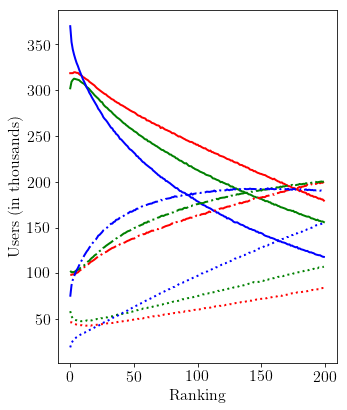
Figure 2. Ranking evolution of short (solid lines), medium (dash lines) and long–tail (dots) items within the top-200 recommendations for the Netflix dataset. MIL lin-sig  model is presented in blue lines, CE_Point lin-sig  in red, and MULTI tanh-lin  in green.

We finally analyze in Figure 2 how items belonging to the short (solid lines), medium (dash lines) or long–tail (dots) popularity intervals are ranked within the top-200 recommendations, for the Netflix dataset. As observed, the CE_Point lin-sig  model attacks mainly short–tail items for ranking positions smaller than $100$ (red solid line). This explains the competitive metric scores reported in Table 3, as well as the relatively few items set with a high preference, see Table 6. On the other hand, the Multi (green) model reduces the number of popular items ranked in the top positions, while recommending more items from the medium and long–tail. This change from short– towards medium and long–tail recommendations may explain the relatively poorer performance of the multinomial loss at small top-$k$ values.

The CE_Point lin-sig  model tends to under-represent infrequent items (red dots). This misrepresentation of long–tail items is alleviated by MIL models. They heavily set short-tail items at the very top of the ranking (blue solid lines), but drastically reduce their appearance shortly thereafter. Instead, MIL models sharply increase the recommendation of medium–tail items (blue dash lines) until the top-100 ranking, where the growth rate stagnates. Meanwhile, for items belonging to the long–tail (blue dots), MIL expands its appearance almost linearly, to the point that they exceed the number of short–tail recommendations. We finally highlight that for ranking position $100$, MIL lin-sig  recommends long–tail items to $\sim 40k$ users more than CE_Point lin-sig  and $\sim 25k$ users more than MULTI tanh-lin.

5. Conclusions and next steps

In this paper we present a novel objective function, the Missing Information Loss (MIL), specifically designed for handling unobserved user-item interactions in implicit feedback datasets. In particular, MIL explicitly forbids treating missing user-item interactions as positive or negative feedback. We demonstrate that, thanks to the functional form of the MIL function, the ranking of unseen items is almost entirely left to the low–rank process, rather than forcing unobserved items to be at the tail of the recommendation (i.e., MIL does not force a zero predicted preference for unobserved user-item interactions).

Extensive experiments with Matrix Factorization and Denoising Autoencoders conducted on three datasets, show that MIL models demonstrate competitive performance when compared with other traditional losses such as cross-entropy or the multinomial log-likelihood. In addition, we study the distribution of the recommendations and observe that the reported metric performance takes place while recommending popular items less frequently (up to a $20\%$ decrease with respect to the best competing method). Indeed, MIL models sharply increase the recommendation of medium–tail items, while almost linearly expanding the appearance of long–tail items with the ranking position in the list of recommendations. Such expansion results in up to a $50\%$ increase of long–tail recommendations, a feature of utmost importance for industries with a large catalogue of items.

Future lines of research may involve the incorporation of negative feedback, or the usage of MIL in temporal–aware Recommender Systems (such as those using Recurrent Neural Networks). In addition, we hope that the results here reported will bring forward first-principle mathematical derivations of the MIL function, so that the vast family of possible polynomials modelling the missing information term can be reduced, or even extended with more suitable functions.

- [1] Chris Anderson. The Long Tail: Why the Future of Business Is Selling Less of More. Hyperion, 2006.
- [2] Harald Steck. Item popularity and recommendation accuracy. In Proceedings of the Fifth ACM Conference on Recommender Systems, RecSys ’11, pages 125–132, New York, NY, USA, 2011. ACM.
- [3] Yifan Hu, Yehuda Koren, and Chris Volinsky. Collaborative filtering for implicit feedback datasets. In 2008 Eighth IEEE International Conference on Data Mining, pages 263–272, Dec 2008.
- [4] Rong Pan, Yunhong Zhou, Bin Cao, Nathan N. Liu, Rajan Lukose, Martin Scholz, and Qiang Yang. One-class collaborative filtering. In Proceedings of the 2008 Eighth IEEE International Conference on Data Mining, ICDM ’08, pages 502–511, Washington, DC, USA, 2008. IEEE Computer Society.
- [5] Harald Steck. Training and testing of recommender systems on data missing not at random. In Proceedings of the 16th ACM SIGKDD International Conference on Knowledge Discovery and Data Mining, KDD ’10, pages 713–722, New York, NY, USA, 2010. ACM.
- [6] Dawen Liang, Rahul G. Krishnan, Matthew D. Hoffman, and Tony Jebara. Variational autoencoders for collaborative filtering, 2018. cite arxiv:1802.05814Comment: 10 pages, 3 figures. WWW 2018.
- [7] Pascal Vincent, Hugo Larochelle, Yoshua Bengio, and Pierre-Antoine Manzagol. Extracting and composing robust features with denoising autoencoders. In Proceedings of the 25th International Conference on Machine Learning, ICML ’08, pages 1096–1103, New York, NY, USA, 2008. ACM.
- [8] Yao Wu, Christopher DuBois, Alice X. Zheng, and Martin Ester. Collaborative denoising auto-encoders for top-n recommender systems. In Proceedings of the Ninth ACM International Conference on Web Search and Data Mining, WSDM ’16, pages 153–162, New York, NY, USA, 2016. ACM.
- [9] Mark A. Kramer. Nonlinear principal component analysis using autoassociative neural networks. AIChE Journal, 37(2):233–243, 1991.
- [10] Suvash Sedhain, Aditya Krishna Menon, Scott Sanner, and Lexing Xie. Autorec: Autoencoders meet collaborative filtering. In Proceedings of the 24th International Conference on World Wide Web, WWW ’15 Companion, pages 111–112, New York, NY, USA, 2015. ACM.
- [11] Steffen Rendle, Christoph Freudenthaler, Zeno Gantner, and Lars Schmidt-Thieme. Bpr: Bayesian personalized ranking from implicit feedback. In Proceedings of the Twenty-Fifth Conference on Uncertainty in Artificial Intelligence, UAI ’09, pages 452–461, Arlington, Virginia, United States, 2009. AUAI Press.
- [12] Vinod Nair and Geoffrey E. Hinton. Rectified linear units improve restricted boltzmann machines. In Johannes Fürnkranz and Thorsten Joachims, editors, Proceedings of the 27th International Conference on Machine Learning (ICML-10), pages 807–814. Omnipress, 2010.
- [13] O. Celma. Music Recommendation and Discovery in the Long Tail. Springer, 2010.
- [14] Saúl Vargas and Pablo Castells. Rank and relevance in novelty and diversity metrics for recommender systems. In Proceedings of the Fifth ACM Conference on Recommender Systems, RecSys ’11, pages 109–116, New York, NY, USA, 2011. ACM.
- [15] Martín Abadi, Ashish Agarwal, Paul Barham, Eugene Brevdo, Zhifeng Chen, Craig Citro, Greg S. Corrado, Andy Davis, Jeffrey Dean, Matthieu Devin, Sanjay Ghemawat, Ian Goodfellow, Andrew Harp, Geoffrey Irving, Michael Isard, Yangqing Jia, Rafal Jozefowicz, Lukasz Kaiser, Manjunath Kudlur, Josh Levenberg, Dan Mané, Rajat Monga, Sherry Moore, Derek Murray, Chris Olah, Mike Schuster, Jonathon Shlens, Benoit Steiner, Ilya Sutskever, Kunal Talwar, Paul Tucker, Vincent Vanhoucke, Vijay Vasudevan, Fernanda Viégas, Oriol Vinyals, Pete Warden, Martin Wattenberg, Martin Wicke, Yuan Yu, and Xiaoqiang Zheng. TensorFlow: Large-scale machine learning on heterogeneous systems, 2015. Software available from tensorflow.org.
- [16] Xavier Glorot and Yoshua Bengio. Understanding the difficulty of training deep feedforward neural networks. In International conference on artificial intelligence and statistics, AISTATS 2010, pages 249–256, 2010.
- [17] Diederik P. Kingma and Jimmy Ba. Adam: A method for stochastic optimization. CoRR, abs/1412.6980, 2014.
- [18] Dawen Liang, Jaan Altosaar, Laurent Charlin, and David M. Blei. Factorization meets the item embedding: Regularizing matrix factorization with item co-occurrence. In Proceedings of the 10th ACM Conference on Recommender Systems, RecSys ’16, pages 59–66, New York, NY, USA, 2016. ACM.
- [19] Harald Steck. Gaussian ranking by matrix factorization. In Proceedings of the 9th ACM Conference on Recommender Systems, RecSys ’15, pages 115–122, New York, NY, USA, 2015. ACM.
- [20] Òscar Celma and Perfecto Herrera. A new approach to evaluating novel recommendations. In Proceedings of the 2008 ACM Conference on Recommender Systems, RecSys ’08, pages 179–186, New York, NY, USA, 2008. ACM.